Asymptotic Gauge Symmetry in Rindler Coordinates
with Canonical Quantized U(1) Gauge Field

Shingo Takeuchi

Institute of Research and Development, Duy Tan University, Da Nang, Vietnam
Faculty of Environmental and Natural Sciences, Duy Tan University, Da Nang, Vietnam

In the former part of this study, the canonical quantization of U(1) gauge field is performed in the Rindler system, in the Lorentz covariant gauge. This has not been performed yet, while that of scalar and spinor fields have been done. Then, using that result, the Unruh temperature of the U(1) gauge field is analyzed. In the later part of this study, that the acceleration becomes zero on the Killing horizon in the Rindler coordinates is pointed out. Then based on this, it is shown that the infinite symmetries, analogous to the asymptotic gauge symmetry in the infinite null region of the flat spacetime, exist on the Killing horizon in the Rindler system, and a Ward identity of those and the scattering amplitude including soft photons are equivalent to each other. These infinite gauge symmetries in the Rindler system have not been known yet, and are interesting as new asymptotic symmetry and in terms of the holographic dual CFT.

1 Introduction

From the analysis for time-like Killing vectors and the structure of ground states in the Minkowski spacetime with the Killing horizons, the Fulling-Davis-Unruh temperature is derived as $T_{U}=\hbar a/(2\pi ck_{\rm B})\approx 4\times 10^{-23}\,a/$(cm/$s^{2}$) [K] [Fulling:1972md, Davies:1974th, Unruh:1976db]. Therefore, what we can produce currently is no more than noises in the $3$[K] CMB, and becoming possible to observe it is a technological issue for the current us. In addition, it is also important as the experimental confirmation of the Hawking radiation. As the recent main studies in the experimental field, the author refers to the following ones: BEC [Retzker], neutrino oscillation [Luciano:2021onl, Cozzella:2018qew, Dvornikov:2015eqa] anti-Unruh effect [Pan:2023tqb, Pan:2021nka, Chen:2021evr, Zhou:2021nyv, Barman:2021oum, Li:2018xil, Garay:2016cpf, Liu:2016ihf, Brenna:2015fga], cold atoms [Kosior:2018vgx, Rodriguez-Laguna:2016kri], Berry phases [Quach:2021vzo, Martin-Martinez:2010gnz], Casimir effects [Lin:2018wxu, Marino:2014rfa], classical analog [Leonhardt:2017lwm] and others [Lynch:2019hmk, Lochan:2019osm].

Theoretically, the coordinates of a constant accelerated motion are generalized to the Rindler one, in which the Killing horizons exist, which is supposed to be analogous to the event-horizon. As a result, it is considered that the thermal excitation analogues to the Hawking radiation is arisen in the Rindler system, which leads to thermal phase transitions [Hill:1986ec, Ohsaku:2004rv, Ebert:2006bh, Castorina:2007eb, Castorina:2012yg, Takeuchi:2015nga], radiation [Schutzhold:2006gj, Schutzhold:2009scb][Iso:2010yq, Iso:2013sm, Oshita:2015xaa, Oshita:2015qka, Iso:2016lua, Yamaguchi:2018cqw], Schwinger effect [Parentani:1996gd, Kim:2016dmm, Kaushal:2022las] and corrections by Unruh effect [Prokhorov:2019cik, Prokhorov:2019hif, Prokhorov:2019yft, Prokhorov:2019sss]. in the Rindler system. Fermi-Dirac statistics of Bose radiation [Ooguri:1985nv] is also intriguing. In addition, by the existence of the Killing horizons, the Rindler system is exploited to examine holographic issues: Einstein equation as a state equation [Jacobson:1995ab], Bousso bound [Pesci:2007rp], Hawking radiation by quantum tunneling [Kim:2007ep] and Rindler-AdS/CFT [Parikh:2012kg, Fareghbal:2014oba, Sugishita:2022ldv].

However, in these, it can be found that the canonical quantization of the gauge fields has not been performed, while scalar and spinor fields have been done [Higuchi:2017gcd][Soffel:1980kx, Ueda:2021nln]. As the works treating the U(1) gauge field in the Rindler system, [Moretti:1996zt, Lenz:2008vw, Zhitnitsky:2010ji, Soldati:2015xma, Blommaert:2018rsf, Mao:2022wfx] are found. Looking at these, it can be found that those other than [Moretti:1996zt] are irrelevant as the study to treat 4D canonical quantization of the U(1) gauge field. So looking [Moretti:1996zt], it can be found that the normalized modes in its Sec.3 are not right and useless. This is because it is not what has been analytically obtained, and different from what we have analytically obtained which are noted in Sec.3 of this paper. In [Moretti:1996zt], only Eq.(79) is given, however the normalization constants cannot be determined only with that; in order for that, 4 formulas are needed as in Appendix.LABEL:r3g67kb in this paper. In addition, its description is not sorted out, so unreliable as a whole.

One of the main reasons for this seems that the integrates in Appendix.LABEL:r3g67kb have been unclear. Those are indispensable in determining the normalization constants of the field, but not included even in [Gradshteyn:1943cpj] ((LABEL:wreh11) is contained, but its definition range is out of what is needed). In this study, integrating those out as in Appendix.LABEL:r3g67kb, we perform the canonical quantization regarding the U(1) gauge field.

If that can be done, as one of the issues to become possible, we become able to obtain the Ward identities for the asymptotic gauge symmetry on the Killing horizon in the Rindler system (KHRS), which is analogous to that in the infinite null region in the flat spacetime [Strominger:2013lka, He:2014cra, He:2015zea, Kapec:2015ena, Campiglia:2015qka][Strominger:2017zoo]. This is because, in this study (Sec.2.4), it is pointed out that the geometry of the region on the KHRS is the same with the infinite null region in the flat spacetime. (Phenomenology, analysis concerning photon antibunchings in the accelerated system would become possible [Giovannini:2010xg]).

In the references above, the Ward identities of those can link to the scattering amplitudes including soft photons, which are supposed to be the NG bosons regarding those, and the existence of which mean the SSB of those. As some of the developments in this literature, the following are referred [Mao:2021eor, Liu:2021dyq, Mao:2021kxq, Zhang:2021nkx, Liu:2022uox, Cheng:2022xyr, Cheng:2022xgm][Banerjee:2017jeg, AtulBhatkar:2018kfi, AtulBhatkar:2019vcb, AtulBhatkar:2020hqz, AtulBhatkar:2021txo, AtulBhatkar:2021sdr, Bhatkar:2022qhz].

Gravitationally, those have been firstly treated in [Bondi:1962px, Sachs:1962wk], and in [Barnich:2009se] it is shown that that is given by the direct product by the Virasolo symmetry on the conformal sphere there and the supertranslation along the retarded/advanced time direction at that conformal sphere. The Ward identities of those and the equivalence to the scattering amplitudes including soft-gravitations are studied in [Strominger:2013jfa, He:2014laa, Cachazo:2014fwa, Kapec:2014opa, Kapec:2016jld, He:2017fsb, He:2019jjk][Strominger:2017zoo]. As well as AdS/CFT [Maldacena:1997re], Kerr/CFT [Guica:2008mu] and so on, the existence of the asymptotic symmetry in the flat spacetime suggests the existence of some holographic dual CFT regarding the flat spacetime, and those scattering amplitudes are important in analyzing that concretely. Actually, those develop to the study of the 2D holographic dual CFT for the flat spacetime, on ${\cal CS}^{2}$ [Bagchi:2016bcd, Pasterski:2016qvg, Cardona:2017keg, Pasterski:2017kqt, Pasterski:2017ylz][Raclariu:2021zjz, Pasterski:2021rjz]. Also, the direction to solve the information paradox by those is considered [Hawking:2016msc, Hawking:2016sgy, Strominger:2017aeh][Chakraborty:2017pmn, Marolf:2017jkr, Compere:2019ssx].

Therefore in the later part of this paper, obtaining a Ward identity for the asymptotic gauge symmetry on the KHRS, we do to the point to show the equivalence between that and the scattering amplitude with a soft photon. That in the Rindler system have not been found out yet, and is interesting. Also, it is interesting in terms of the holographic dual CFT and the information paradox with the soft hairs.

We mention the organization of this paper. In Sec.2, the Rindler coordinate system is reviewed. As the important points, in Sec.2.3, it is pointed out that the acceleration $a$ is zero on the KHRS, based on which, in Sec.2.4, it is pointed out that that region can be patched with the Penrose type coordinates, which plays a critical role in Sec.LABEL:rteyh.

In Sec.3, the canonical quantization of U(1) gauge field is performed in the Rindler system, in the Lorentz covariant gauge. In Sec.3.1, the gauge fixed Lagrangian is obtained. In Sec.3.2 and 3.3, Fourier modes of the fields and the normalization constant of those are obtained. In Sec.3.4, the canonical quantization is performed. In Sec.3.5 and LABEL:utempu1rc, polarization vectors and the solutions at $k_{\perp}=0$ are discussed.

In Sec.LABEL:utempu1rc, the Unruh temperature that the U(1) gauge field arises is obtained. In Sec.LABEL:usdvea, the expression of ${\bm{a}}^{{\rm(M)}\perp}_{\vec{q}}$ (that of the U(1) gauge field) is obtained. In Sec.LABEL:ugfred, obtaining the coefficients of that, that’s the Bogoliubov coefficients, that is concretely obtained. In Sec.LABEL:eppwte, from ${\bm{a}}^{{\rm(M)}\perp}_{\vec{q}}|0_{\rm M}\rangle=0$, the Unruh temperature is obtained.

In Sec.LABEL:rteyh, the existence of the infinite gauge symmetries, analogous to the asymptotic gauge symmetry in the infinite null region of the flat spacetime, is shown on the KHRS and one of those Ward identities and the scattering amplitude including a soft photon are equivalent to each other. In Sec.LABEL:rrt65i, the electric field is defined consistently on the whole KHRS. In Sec.LABEL:bneir and LABEL:brewgb, the charges for the infinite gauge symmetries and the hard and soft ones of those are defined. In Sec.LABEL:tjreg, a Ward identity for those charges is analyzed and shown that it can be reduced to the scattering amplitude including a soft photon using the result of the soft theorem. In Sec.LABEL:lokiw, it is shown that the Ward identity itself can be reduced to the same result in Sec.LABEL:lokiw not using the soft theorem.

In Sec.LABEL:Summary, summary comments of this work are given. In Appendix.LABEL:drespt, it is shown that the $\beta$ in the Euclid Rindler system is identified to the temperature. In Appendix.LABEL:buobhs, the part in the analysis in Sec.3.1, which is found in the usual textbooks, is described. In Appendix,LABEL:r3g67kb, the integral formulas used in Sec.3.3 are given.

2 Review of Rindler coordinate system

In this study, we exploit the Rindler coordinate system. Therefore, in this section, we review the Rindler coordinate system in detail.

2.1 Rindler coordinate system

We begin with the 4D Minkowski spacetime given as

$$ds^{2}=c^{2}dt^{2}-(dx^{1})^{2}-(dx^{2})^{2}-(dx^{3})^{2}.$$ (1)

We consider an object performing a constant accelerated motion with an acceleration $a$ for the $x^{1}$-direction. Solving $\frac{d}{dt}(\frac{mv}{\sqrt{1-\beta^{2}}})=ma$ ($\beta=v/c$) with the condition $v=0$ at $t=0$, we can get $v=at\sqrt{1-\beta^{2}}$. Then, from the proper time $\tau=\int_{0}^{t}dt\sqrt{1-\beta^{2}}$ and $x^{1}=\int^{t}_{0}dt\,v$, we can obtain the trajectory of the accelerated motion as follows:

$$t=\frac{c}{a}\sinh\frac{a\tau}{c},\quad x^{1}=\frac{c^{2}}{a}\,(\cosh\frac{a\tau}{c}-1).$$ (2)

Based on (2), we consider the following Rindler coordinate system given with $(\tau,\xi)$:

$$t=\frac{c}{a}\,e^{a\xi/c^{2}}\sinh\frac{a\tau}{c},\quad x^{1}=\frac{c^{2}}{a}\,e^{a\xi/c^{2}}\cosh\frac{a\tau}{c}.$$ (3)

In the coordinate system $(\tau,\xi)$, $a$ is just a parameter, however $a$ still has the meaning of the acceleration as its physical meaning.

Actually, around $a=0$, $t$ and $x^{1}$ in (3) are given as: $t=\tau+{\cal O}(a)$ and $x^{1}=c^{2}/a+\xi+{\cal O}(a)$. If we remember that “$-c^{2}/a$” is dropped in getting (3) from (2), $x^{1}$ becomes constant and consistent with the physical meaning. $c$ is $1$ in what follows.

Figure 1: This represents the Rindler coordinate system (10). $\tau$, $\xi$ and so on are not written in to avoid the figure to get messy. The straight diagonal lines in RRW are the $\xi\to-\infty$ lines, on which $\tau$ is $+\infty$ or $-\infty$ for $t>0$ or $t<0$ except for the origin.

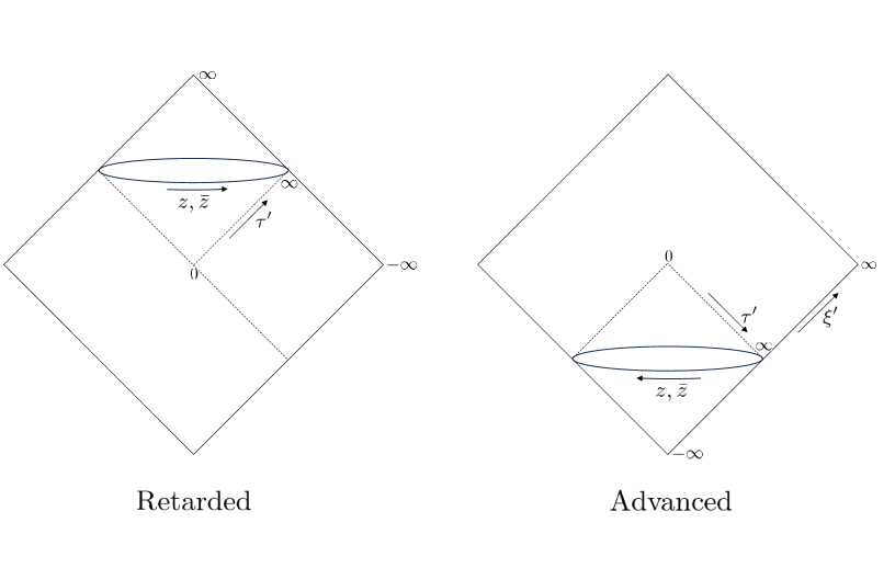
Figure 2: These represent the Penrose diagram type coordinates (23). Correspondence relation with the Rindler coordinates in Fig.1 is given in (24).

2.2 $ds^{2}$ in Rindler coordinate system

The definition ranges of the time-like Rindler coordinates are given as

$$0<x^{1}<\infty, \quad-x^{1}<t<x^{1},\quad\textrm{for $a>0$,}$$ (4a)

$$-\infty<x^{1}<0, \quad-x^{1}>t>x^{1},\quad\textrm{for $a<0$.}$$ (4b)

These are space-likely separated from each other, which leads to the left (LRW) and right Rindler-wedges (RRW). In either side, the ranges of $\tau$ and $\xi$ are given as follows:

$$-\infty<\tau<\infty,\quad-\infty<\xi<\infty.$$ (5)

By (3) we can write as $ds^{2}=e^{2a\xi}(d\tau^{2}-d\xi^{2})$. From this, we can see the $\tau$-direction is a Killing vector, which can be given in the Minkowski coordinate system as

$$\xi_{\rm R}\equiv a(z\partial_{t}+t\partial_{1}).$$ (6)

Since $\xi_{\rm R}^{2}=a^{2}((x^{1})^{2}-t^{2})$, $\xi_{\rm R}$ is time-like in the LRW and RRW.

(3) can cover only the RRW. The coordinates covering the LRW is given as

$$t=a^{-1}e^{a\tilde{\xi}}\sinh a\tilde{\tau},\quad x^{1}=-a^{-1}e^{a\tilde{\xi}}\cosh a\tilde{\tau}.$$ (7)

With (3) and (7), it can be written as

$$ds^{2}=\left\{\begin{array}[]{ll}\!e^{2a\tilde{\xi}}(d\tilde{\tau}^{2}-d\tilde{\xi}^{2})-(dx^{\perp})^{2}\equiv ds^{2}_{{\rm LRW}}&\!\textrm{for LRW},\\[4.2679pt] \!e^{2a\xi}(d\tau^{2}-d\xi^{2})-(dx^{\perp})^{2}\equiv ds^{2}_{{\rm RRW}}&\!\textrm{for RRW},\end{array}\right.$$ (10)

where we used the notation $x^{\perp}\equiv(x^{2},x^{3})$.

2.3 $\xi\to-\infty$ line

In Sec.LABEL:rteyh of this study, we address the issue of the asymptotic gauge symmetry in the Rindler coordinate system, in which the region of the $\xi\to-\infty$ line plays a very important role. Therefore, we discuss the situation at $\xi\to-\infty$. From (3), we can see that

• • at any points in $t>0$ or $t<0$ on the $\xi\to-\infty$ line, it should be that $|\tau|>|\xi|$, otherwise neither of $t$ nor $z$ in (3) can be finite. Therefore, on the $\xi\to-\infty$ line, $\tau$ is supposed as follows:

    $$\tau\to\left\{\begin{array}[]{ll}\displaystyle\!\!+\infty&\!\!\!\textrm{for $t>0$,}\\[4.2679pt] \displaystyle\!\!-\infty&\!\!\!\textrm{for $t<0$.}\end{array}\right.$$ (13)

  • Therefore, if $\tau$ is always $\infty$ or $-\infty$ in $t>0$ or $t<0$ on the $\xi=-\infty$ line, $t/x^{1}=\tanh(a\tau)$ is $+1$ or $-1$. Therefore, the $\xi\to-\infty$ line is the $\pm 45$ degrees straight diagonal lines going to or coming out from the origin, which is the null line corresponding to the trajectory of a light.

  • Therefore, the velocity on the $\xi\to-\infty$ line is supposed as

    $$v\to\left\{\begin{array}[]{ll}\displaystyle\!\!+c&\!\!\!\textrm{for $t>0$,}\\[4.2679pt] \displaystyle\!\!-c&\!\!\!\textrm{for $t<0$.}\end{array}\right.$$ (16)

  • Therefore, on the $\xi\to-\infty$ line, the motion of the object is the uniform linear motion, and $a$ can be put as

    $$a\to 0 \xi\to-\infty$$   at   . (17)

  • Therefore, from (10), on the $\xi\to-\infty$ line, the U(1) gauge field can be given by the free one in the inertial system. This point is critical in Sec.LABEL:lokiw.

• At this time, the front factor in (10), $e^{2a\xi}$ ($e^{2a\tilde{\xi}}$), gets to $1$. On the other hand of this, $ds^{2}$ should be $0$ on the $\xi\to-\infty$ line.

  Regarding this, first of all, motions with any $a$ asymptote to the $\xi\to-\infty$ line at $|\tau|\to\infty$. From this fact, trajectories of those at $|\tau|\to\infty$ can be effectively identified to the $\xi\to-\infty$ line. From this fact, it is supposed that on the $\xi\to-\infty$ line, $ds^{2}$ vanishes regardless of $a$.

  Here, let us note that $t$ and $z$ in (10) grow exponentially in $|\tau|\to\infty$. From this fact, it is concluded that in the finite section on the $\xi\to-\infty$ line, the value of $\tau$ ($\tilde{\tau}$) is unchangeable, in effect, for any $a$. By this, it can realize that

  $$ds^{2}=0 \xi\to-\infty$$   at   , (18)

  where since $a$ is constant, $\xi$ is constant.

• Lastly, the motion of the object in finite $\tau$ on the $\xi\to-\infty$ line is all packed into the one point of the origin.

On the other hand, no issues are found to be discussed in particular in other extremal values such as $\xi\to 0$ or $+\infty$.

2.4 Penrose type coordinate system

In this subsection, we mention another critical point in Sec.LABEL:rteyh. As mention in (17), when $\xi\to-\infty$ is considered, it is that $a\to 0$ in $ds^{2}_{{\rm RRW}}$ (10). In that situation, giving it as

$$ds^{2}_{{\rm RRW}}=d\tau^{2}-dr^{2}-r^{2}d\Omega^{2}\quad(r^{2}=\xi^{2}+(x^{\perp}){}^{2}),$$ (19)

we apply

$$\tau=\eta\pm r,\quad\xi=\pm r\frac{1-z\bar{z}}{1+z\bar{z}},\quad x^{2}+ix^{3}=\pm\frac{2rz}{1+z\bar{z}}$$ (20)

to that, where $+/-$ are taken for $t\geq 0$ and $\leq 0$. As a result, we can obtain as

$$ds^{2}_{\rm RRW}=\left\{\begin{array}[]{ll}\!d\eta^{2}+2d\eta dr-2r^{2}\gamma_{z\bar{z}}dzd\bar{z}&\!\textrm{for $t>0$},\\[4.2679pt] \!d\eta^{2}-2d\eta dr-2r^{2}\gamma_{z\bar{z}}dzd\bar{z}&\!\textrm{for $t<0$},\end{array}\right.$$ (23)

where $\gamma_{z\bar{z}}\equiv\frac{2}{(1+z\bar{z})^{2}}$. LRW is likewise. We list points in (23) in what follows.

• We check the correspondence relation between (10) and (23). First, we show the spacetime patched with (23) in Fig.2.

  • The “Retarded” and “Advanced” are applied to the $t>0$ and $t<0$ respectively. The origin is not covered.

  • Which parts in (19) map to which parts in (23) can be gotten from the following relationships for the overlapping in the coordinate patchings:

    $$\,\textrm{$\tau$ line in $t>0$ and $<0$}\,\,\xrightarrow[\textrm{overlaps}]{}\,\textrm{$\eta$ line in Retarded and Advanced.}$$ (24)

  • From (24), it can be seen that $\eta$ does not correspond to the retarded/advanced times existing in the original Penrose coordinates.

• • In $\xi\to-\infty$, $\xi$ mostly overlaps $\tau$ and those are parallel to each other, while $\eta$ is taken to be exactly parallel to $\tau$.

  • $\eta$ takes values in the following manner:

    $$\eta=\left\{\begin{array}[]{ll}\!\tau-r,&\!\textrm{where $\tau,\,\xi\to+\infty,\,-\infty$ in $t>0$,}\\[4.2679pt] \!\tau+r,&\!\textrm{where $\tau,\,\xi\to-\infty,\,-\infty$ in $t<0$.}\end{array}\right.$$ (27)

  • Since the $\tau$-axis is a time-like Killing vector, the parametrization on that is linked to the structure of the ground state, and is crucial in treating issues of the accelerated system. Therefore, let us mention that by (20), the parametrization on the $\eta$ line is not changed from the one on $\tau$ line; only uniformly displaced for some constant. Therefore, by in (20), the structure of the ground state is not changed.

• • (23) is applicable only for the region on the $\xi\to-\infty$ line. This is because $a$ can be zero as in (17) only on the $\xi\to-\infty$ line.

  • Let us just comment that at arbitrary $a$, it is possible to transform the Rindler coordinates to the Penrose ones by once getting it back to the Minkowski coordinates. However, it is meaningless as the accelerated system. This is because the coordinates of that are basically given by $(t,z)\sim(\sinh\tau,\cosh\tau)$ as in (3), and except at $a=0$, there is no way to apply those to the Penrose coordinates. This means that except at $a=0$, the Penrose coordinates do not correspond to the accelerated system.

• By $z\to-1/\bar{z}$, the two in (23) can interchange with each other. However, $z\to-1/\bar{z}$ maps a point to the antipodal point of that on the sphere. Therefore, the left and right in the two in (23) are in the other way around each other. Therefore, unlike (16), in the coordinate system (23), $v$ can be held as

  $$v=\left\{\begin{array}[]{ll}\!+c,&\!\textrm{in $t>0$,}\\[4.2679pt] \!+c,&\!\textrm{in $t<0$.}\end{array}\right.$$ (30)

  In Sec.LABEL:rteyh, by employing the Penrose type coordinates (27), $v$ in (30) is considered, which is another critical point in defining the charges in Sec.LABEL:bneir.

2.5 Light-cone coordinate system

We define the light-cone coordinates in the Minkowski coordinate system as follows:

$$U\equiv t-z,\quad V\equiv t+z.$$ (31)

From Fig.1, we can see that

$$U\left\{\begin{array}[]{ll}\!>0&\!\textrm{in LRW,}\\[4.2679pt] \!<0&\!\textrm{in RRW,}\end{array}\right.\quad V\left\{\begin{array}[]{ll}\!<0&\!\textrm{in LRW,}\\[4.2679pt] \!>0&\!\textrm{in RRW.}\end{array}\right.$$ (36)

Based on (3) and (7), we can represent these in terms of the LRW and RRW coordinates ($\tilde{\tau}$, $\tilde{\xi}$) and ($\tau$, $\xi$) as follows:

$$(U,V)=\left\{\begin{array}[]{ll}\!a^{-1}(e^{a\tilde{u}},\,-e^{-a\tilde{v}})&\!\textrm{in LRW,}\\[4.2679pt] \!a^{-1}(-e^{-au},\,e^{av})&\!\textrm{in RRW,}\end{array}\right.$$ (39)

where $(\tilde{u},\tilde{v})\equiv(\tilde{\tau}-\tilde{\xi},\tilde{\tau}+\tilde{\xi})$ and $(u,v)\equiv(\tau-\xi,\tau+\xi)$.

2.6 Unruh temperature

Let us introduce a coordinate $\rho$ defined as follows:

$$\rho\equiv\left\{\begin{array}[]{ll}\!-a^{-1}e^{a\tilde{\xi}}&\!\textrm{in LRW,}\\[4.2679pt] \!+a^{-1}e^{a\xi}&\!\textrm{in RRW.}\end{array}\right.$$ (42)

Then, $ds^{2}$ in (10) can be written commonly for LRW and RRW as follows:

$$ds^{2}=a^{2}\rho^{2}d\tau^{2}-d\rho^{2}-(dx^{\perp})^{2}.$$ (43)

Let us Euclideanize the $\tau$ as $\tau\to i\tau$ in (43). Then (43) can be written as

$$ds^{2}_{\rm E}=a^{2}\rho^{2}d\tau^{2}+d\rho^{2}+(dx^{\perp})^{2},$$ (44)

where $ds^{2}_{E}\equiv-ds^{2}$. In (44), the $\tau$-direction is periodic by $\beta\equiv 2\pi/a$, the inverse of which agrees with the temperature in the accelerated system. We review it in Appendix.LABEL:drespt.

3 Canonical quantization of U(1) gauge field in Rindler coordinate system

In this section, we perform the canonical quantization of the U(1) gauge field in Rindler coordinate system.

3.1 Lagrangian of U(1) gauge field in Lorentz covariant gauge in Rindler coordinate system

We consider the following Lagrangian density of U(1) gauge field on (10):

$$S=\int_{\rm RRW}\!d^{4}x\,\sqrt{-g}\,{\cal L}_{\rm U(1)},\quad{\cal L}_{\rm U(1)}=-F_{\mu\nu}F^{\mu\nu}/4,$$ (45)

where $\nabla_{\mu}$ are covariant derivatives given by the metrices (10), and $F_{\mu\nu}=\nabla_{\mu}A_{\nu}-\nabla_{\nu}A_{\mu}=\partial_{\mu}A_{\nu}-\partial_{\nu}A_{\mu}$. We obtain the Lagrangian in the Lorentz covariant gauge. Here, the following Christoffel symbols exist non-zero in the Rindler coordinate system:

$$\Gamma^{0}_{01}=\rho^{-1},\quad\Gamma^{1}_{00}=a^{2}\rho,\quad\textrm{others $=0$}.$$ (46)

Here, the Lagrangian in the Lorentz covariant gauge can be obtained in the Minkowski coordinate system as follows:

$$T\!\!\! = \!\!\!\int\!{\cal D}\!A^{k}\,{\cal D}B\,{\cal D}c\,{\cal D}\bar{c}\,\exp[\,i\!\int_{\rm RRW}\!d^{4}x\,\sqrt{-g}\,{\cal L}^{tot}],$$ (47)

$${\cal L}^{tot}\!\!\! \equiv \!\!\!{\cal L}_{\rm U(1)}+B\,\partial_{\mu}A^{\mu}+B^{2}/2+i\,\bar{c}\,\partial_{\mu}\partial^{\mu}\,c,$$

where $\nabla_{\mu}A^{\mu}={\cal C}$ is taken as the Lorentz covariant gauge (${\cal C}$ is some real number function). From this, by replacing the differentials with the covariant derivatives (and $d^{4}x$ with $d^{4}x\,\sqrt{-g}$), we can obtain the Lagrangian in the Lorentz covariant gauge in the Rindler coordinate system as follows:

$${\cal L}^{tot}\!\!\! \equiv \!\!\!{\cal L}_{\rm U(1)}+B\,\nabla_{\mu}A^{\mu}+B^{2}/2+i\,\bar{c}\,\nabla_{\mu}\nabla^{\mu}\,c,\quad$$ (48)

and all fields have the canonical conjugate momentum as follows:

$$\bullet\quad\frac{\partial{\cal L}^{tot}}{\partial(\nabla_{0}A^{k})}=F_{k}{}^{0}\equiv\pi_{k},\quad\frac{\partial{\cal L}^{tot}}{\partial(\nabla_{0}A^{0})}=B=-\nabla_{\mu}A^{\mu}\equiv\pi^{(0)},\quad$$

$$\bullet\quad\,\,\frac{\partial{\cal L}^{tot}}{\partial(\nabla_{0}B)}=-A^{0}\equiv\pi^{(B)},\quad\frac{\partial{\cal L}^{tot}}{\partial(\nabla_{0}c)}=i\,\nabla^{0}\bar{c}\equiv\pi^{(c)},\quad\frac{\partial{\cal L}^{tot}}{\partial(\nabla_{0}\bar{c})}=-i\,\nabla^{0}c\equiv\pi^{(\bar{c})},$$

where we have performed the differential of the ghost fields with the left-differential. However, there is a question if we can obtain (47). We check this in this subsection.

3.1.1 Hamiltonian

The dynamical variables in the model (45) are $A^{\mu}$, and the conjugate momenta of those are given as follows:

$$\frac{\partial{\cal L}_{\rm U(1)}}{\partial(\partial_{0}A^{\mu})}=g^{00}F_{\mu 0}\equiv E_{\mu}\equiv\pi_{\mu},\quad\frac{\partial{\cal L}_{\rm U(1)}}{\partial(\partial_{0}A_{\mu})}=F^{\mu 0}\equiv E^{\mu}\equiv\pi^{\mu},$$ (50)

where $\pi_{\mu}$ in the one is that in (3.1) for $\mu=k$. Therefore, $\pi_{k}=-\pi^{k}$ and $E_{\nu}=g_{\nu\mu}E^{\mu}$.

We can express the Lagrangian density (45) as follows:

$${\cal L}_{\rm U(1)}\!\!\! = \!\!\!F_{\mu 0}F^{\mu 0}/2-F_{ij}F^{ij}/4$$ (51)

$$= \!\!\!E_{k}(\nabla_{0}A_{k}-\nabla_{k}A_{0})-(B_{k}^{2}+g_{00}E_{k}^{2})/2,$$

where $B^{k}\equiv-\varepsilon^{ijk}F_{ij}/2$ and $B_{k}\equiv\varepsilon_{ijk}F^{ij}/2$.

Regarding the second term in the r.h.s. of (51), we can rewrite as

$$\int_{\rm RRW}\!d^{4}x\sqrt{-g}\,E_{k}\nabla_{k}A_{0}=\int_{\rm RRW}\!d^{4}x\sqrt{-g}\,\nabla_{k}E^{k}A_{0},$$ (52)

where we have assumed that the integral on the spacial surface at the far region vanishes, then used $\nabla_{k}V_{j}=\partial_{k}V_{j}$ for general $V_{j}$ in our study with (46), and $\partial_{\mu}\sqrt{-g}=\sqrt{-g}\,\Gamma^{\alpha}_{\mu\alpha}$. With this, we can write (51) as

$$\textrm{(\ref{bv64r})}=E_{k}\nabla_{0}A_{k}-\nabla_{k}E^{k}A_{0}+(B_{k}^{2}+g_{00}E_{k}^{2})/2.$$ (53)

With (53), the Hamiltonian density can be obtained as follows:

$${\cal H}=\nabla_{0}A_{\mu}\,\pi^{\mu}-{\cal L}_{\rm YM}=2\nabla_{0}A^{k}E_{k}+\nabla_{k}E^{k}A_{0}+\frac{1}{2}(B_{k}^{2}+g_{00}E_{k}^{2}).$$ (54)

We quantize $A^{\mu}$ with the simultaneous commutation relation obtained from the Poisson brackets:

$$\{A^{\mu}(\tau,\vec{x}),\pi_{\nu}(\tau,\vec{y})\}_{{\rm P.B.}}=\delta^{\mu}{}_{\nu}\delta^{3}(\vec{x}-\vec{y}),$$ (55)

where $\{\cdot,\cdot\}_{{\rm P.B.}}$ means Poisson bracket:

$$\{X,Y\}_{{\rm P.B.}}\equiv\frac{\partial X}{\partial A^{\rho}}\frac{\partial Y}{\partial\pi_{\rho}}-\frac{\partial X}{\partial\pi_{\rho}}\frac{\partial Y}{\partial A^{\rho}}.$$ (56)

However, $\pi_{0}$ lacks in the theory (45).

3.1.2 Constitution of path-integral

In the system with the Hamiltonian density (54), there are two constraint conditions $\phi^{(i)}$ $(i=1,2)$:

$$\phi^{(1)}\equiv\pi_{0}=0,\quad\phi^{(2)}\equiv\nabla^{k}\pi_{k}=0.$$ (57)

Toward (57), we take the Coulomb gauge type gauge $\chi^{(i)}$ $(i=1,2)$ as follows:

$$\chi^{(1)}\equiv A^{0}=0,\quad\chi^{(2)}\equiv\nabla_{k}A^{k}=0.$$ (58)

Denoting these together as $\tilde{\phi}\equiv\{\phi^{(1)},\phi^{(2)},\chi^{(1)},\chi^{(2)}\}$, the Poisson bracket for $\tilde{\phi}$ can be obtained for each $\tau$ as follows:

$$\{\tilde{\phi}(x),\tilde{\phi}(y)\}_{\rm P.B.}=\left[\begin{array}[]{cccc}0&0&-1&0\\ 0&0&0&-\nabla^{k}\nabla_{k}\\ 1&0&0&0\\ 0&\nabla^{k}\nabla_{k}&0&0\end{array}\right]\times\delta^{3}(\vec{x}-\vec{y}),$$ (59)

where $x_{0}$ and $y_{0}$ refer to the same $\tau$. Since ${\rm det}\{\tilde{\phi}(x),\tilde{\phi}(y)\}_{\rm P.B.}$ is non-vanishing, $\tilde{\phi}$ is forming a second class constraint. When the conditions (57) and (58) are imposed in the phase space of the $(A^{\mu},\pi_{\mu})$, our path-integral can be written as follows:

$$T\!\!\! \equiv \!\!\!\int\!{\cal D}\!A\,{\cal D}\pi\prod_{x\in{\rm RRW}}\big{[}\delta(\phi^{(1)})\,\delta(\phi^{(2)})\,\delta(\chi^{(1)})\,\delta(\chi^{(2)})\big{]}\cdot\prod_{\tau}\textrm{Det}\big{[}M_{c}(x,y)\big{]}$$ (60)

$$\times\exp\big{[}i\int_{\rm RRW}\!d^{4}x\,\sqrt{-g}\,\{\nabla_{0}A^{\mu}\,\pi_{\mu}-{\cal H}\}\big{]},$$

where

$$M_{c}(x,y) \equiv\{\phi(x),\chi(y)\}_{\rm P.B.}=\nabla^{k}\nabla_{k}\delta^{3}(\vec{x}-\vec{y}),$$ (61a)

$${\cal D}\!A\,{\cal D}\pi \equiv\prod_{\mu=0}^{3}\prod_{x\in{\rm RRW}}dA^{\mu}(x)\,d\pi_{\mu}(x),$$ (61b)

where $\phi\equiv\{\phi^{(1)},\phi^{(2)}\}$ and $\chi\equiv\{\chi^{(1)},\chi^{(2)}\}$.

3.1.3 Constitution of Lagrangian in Lorentz covariant gauge

Let us integrate out $\pi_{0}$ in (60), which can be performed readily as $\phi^{(1)}=\pi_{0}$ as in (57). Then, introducing new variable $\eta=\eta(x)$, we perform the following rewriting:

$$\prod_{x\in{\rm RRW}}\delta(\phi^{(2)})=\int{\cal D}\eta\,\exp\big{[}i\int_{\rm RRW}d^{4}x\,\sqrt{-g}\,\eta\,\phi^{(2)}\big{]}.$$ (62)

Now (60) can be written as follows:

(60) $$= \!\!\!\int\!{\cal D}\!A\,{\cal D}\pi_{k}\int{\cal D}\eta\,\prod_{x\in{\rm RRW}}\big{[}\delta(\chi^{(1)})\,\delta(\chi^{(2)})\big{]}\cdot\prod_{\tau}\textrm{Det}\big{[}M_{c}(x,y)\big{]}$$ (63)

$$\!\!\!\!\times\,\exp\big{[}i\int_{\rm RRW}d^{4}x\,\sqrt{-g}\,\{\nabla_{0}A^{k}\,\pi_{k}-{\cal H}|_{\pi_{0}=0}+\eta\,\nabla^{k}\pi_{k}\}\big{]}.$$

Since ${\cal H}$ does not contain $\pi_{0}$ as can be seen in (54), we write ${\cal H}|_{\pi_{0}=0}$ as ${\cal H}$ in the following.

Now let us integral out $A^{0}$. By that, since $\chi^{(1)}=A^{0}$ as in (58), the second term in the r.h.s. in (54), which is $A_{0}\,\partial_{k}E_{k}$, disappears. However, we can regard $\eta$ with $-A_{0}$ after integrating out of $A^{0}$, by which the term $\eta\,\nabla^{k}\pi^{k}$ in (63) becomes the one that disappeared just now, and ${\cal H}$ given in (54) can revive exactly as it was. Namely,

$$-{\cal H}+\eta\,\nabla^{k}\pi_{k}\!\!\! \xrightarrow[\,\,\,A_{0}\,\to\,0\,\,\,]{} \!\!\![-{\cal H}+\eta\,\nabla_{k}\pi^{k}]\,\big{|}_{A_{0}\,\to\,0}$$ (64)

$$\xrightarrow[\eta\,\to\,-A_{0}]{} \!\!\![-{\cal H}+\eta\,\nabla^{k}\pi_{k}]\,\big{|}_{A_{0}\,\to\,0,\,\eta\,\to\,-A_{0}}=-{\cal H},$$

where we have used $E_{k}\equiv\pi_{k}$ as in (50) in the first line of the one above. As a result, now we can write (63) as follows:

(63) $$= \!\!\!\int\!{\cal D}\!A^{k}\,{\cal D}\pi_{k}\prod_{x\in{\rm RRW}}\big{[}\delta(\chi^{(2)})\big{]}\cdot\prod_{\tau}\textrm{Det}\big{[}M_{c}(x,y)\big{]}$$ (65)

$$\!\!\!\!\times\,\exp\big{[}i\int_{\rm RRW}d^{4}x\,\sqrt{-g}\,(\nabla_{0}A^{k}\,\pi_{k}-{\cal H})\big{]}.$$

In what follows, we show that we can equivalently rewrite $\int_{\rm RRW}d^{4}x\,\sqrt{-g}\,(\nabla_{0}A^{k}\,\pi_{k}-{\cal H})$ to $\int_{\rm RRW}d^{4}x\,\sqrt{-g}\,{\cal L}_{\rm U(1)}$, where ${\cal L}_{\rm U(1)}$ is the one given in (45).

It is that

$$\nabla_{0}A^{k}\,\pi_{k}-{\cal H}=-\nabla_{0}A^{k}\pi_{k}-\nabla_{k}\pi^{k}A_{0}-(B_{k}^{2}+g_{00}\,\pi_{k}^{2})/2.$$ (66)

Here, $-\int_{\rm RRW}d^{4}x\,\sqrt{-g}\,\nabla_{k}\pi^{k}A_{0}=\int_{\rm RRW}d^{4}x\,\sqrt{-g}\,\pi^{k}\nabla_{k}A_{0}$, where we have computed this in the same way with what is written under (52). Then,

(66) $$= \!\!\!F_{k0}\,\pi^{k}-(B_{k}^{2}+g_{00}\,\pi_{k}^{2})/2$$ (67)

$$= \!\!\!\frac{g_{00}}{2}((\pi_{k}+g^{00}F_{0k})(\pi_{k}+g^{00}F_{0k})-(g^{00}F_{0k})^{2})-B_{k}^{2}/2$$

$$= \!\!\!\frac{g_{00}}{2}(\pi_{k}+g^{00}F_{0k})(\pi_{k}+g^{00}F_{0k})-(g^{00}F_{0k}^{2}+B_{k}^{2})/2$$

$$= \!\!\!\frac{g_{00}}{2}(\pi_{k}+g^{00}F_{0k})(\pi_{k}+g^{00}F_{0k})+{\cal L}_{\rm U(1)},$$

where $g^{00}F_{0k}^{2}=g^{00}F_{0k}F_{0k}=-F_{0k}F^{0k}$. We can integrate out $\pi_{k}$ as it is a Gaussian integral. As a result, we can write as

(65) $$= \!\!\!\int\!{\cal D}\!A^{k}\prod_{x\in{\rm RRW}}\big{[}\delta(\chi^{(2)})\big{]}\cdot\prod_{\tau}\textrm{Det}\big{[}M_{c}(x,y)\big{]}\cdot\exp\big{[}i\int_{\rm RRW}d^{4}x\,\sqrt{-g}\,{\cal L}_{\rm U(1)}\big{]}.$$ (68)

From this, we can obtain (47) by proceeding in the same way with the case of the Minkowski coordinate system, which can be found in the usual textbooks. Therefore, we perform the rest in Appendix.LABEL:buobhs.

3.2 Solution of U(1) gauge field in Rindler coordinate system

In this subsection, based on the Lagrangian in (47), we obtain the solution of the U(1) gauge field in the Rindler coordinate system in (43).

3.2.1 Solutions of equations of motion

From (47), the equations of motion can be obtained as follows:

$$0 =-\nabla_{\mu}F^{\mu\nu}+\partial^{\nu}B,$$ (69a)

$$0 =\nabla_{\mu}A^{\mu}+B,$$ (69b)

Combining (69a) and (69b), we can obtain $\nabla_{\nu}\nabla^{\nu}A^{\mu}=0$, which yields (70a)-(70c) (regarding (70b), (70d) is used). From (69b), we can obtain (70d). Multiplying the entire (69a) by $\nabla_{\nu}$, we can obtain $\nabla_{\mu}\nabla^{\mu}B=0$, which yields the following (70e):

$$(g^{\mu\nu}\partial_{\mu}\partial_{\nu}-3\rho^{-1}\partial_{1})A^{0} =-2a^{-2}\rho^{-3}\partial_{0}A^{1},$$ (70a)

$$(g^{\mu\nu}\partial_{\mu}\partial_{\nu}-3\rho^{-1}\partial_{1}-\rho^{-2})A^{1} =-2\rho^{-1}(B-\partial_{\perp}A^{\perp}),$$ (70b)

$$(g^{\mu\nu}\partial_{\mu}\partial_{\nu}-\rho^{-1}\partial_{1})A^{\perp} =0,$$ (70c)

$$\partial_{0}A^{0}+\partial_{1}A^{1}+\partial_{\perp}A^{\perp}+\rho^{-1}A^{1}-B =0,$$ (70d)

$$(g^{\mu\nu}\partial_{\mu}\partial_{\nu}-\rho^{-1}\partial_{1})B =0,$$ (70e)

where $\Gamma^{0}_{01}=\rho^{-1}$, $\Gamma^{1}_{00}=a^{2}\rho$ and others are zero. Here, we are taking the $1$-direction ($\rho$-direction) as the direction of acceleration and $\perp\equiv 2,3$. These can be reduced to the ones in the Minkowski coordinates at $a$ vanishing ($\rho$ is defined in (42)).

Since our Rindler coordinate system is homogeneous for a constant $\rho$ as in (43), we can perform the following plane wave expansion:

$$A^{\mu}(\tau,\rho,x^{\perp}) =\int\!dk_{0}d^{2}k_{\perp}\,\bm{a}^{(\mu)}_{k_{0},k_{\perp}}\,{\cal N}^{(\mu)}_{k_{0}}\,\tilde{A}^{\mu}_{k_{0},k_{\perp}}(\rho)\,e^{-ik_{0}\tau+ik_{\perp}x^{\perp}},$$ (71a)

$$B(\tau,\rho,x^{\perp}) =\int\!dk_{0}d^{2}k_{\perp}\,\bm{b}_{k_{0},k_{\perp}}\,{\cal N}^{(B)}_{k_{0}}\,\tilde{B}_{k_{0},k_{\perp}}(\rho)\,e^{-ik_{0}\tau+ik_{\perp}x^{\perp}},$$ (71b)

where $\int\!{dk_{0}d^{2}k_{\perp}}$ denotes $\int_{0}^{\infty}\!dk_{0}\int_{-\infty}^{\infty}\!d^{2}k_{\perp}$. $\bm{a}^{(\mu)}_{k_{0},k_{\perp}}$ and $\bm{b}_{k_{0},k_{\perp}}$ are some coefficients, and ${\cal N}^{(\mu)}_{k_{0}}$ are the normalization constants, which are obtained in Sec.3.3 (those are turned out to be independent of $k_{\perp}$ and coordinates). Applying these to (70), we can obtain the equations of motion for each mode as follows:

$$((a\rho)^{-2}k_{0}^{2}+\partial_{1}^{2}-k_{\perp}^{2}+3\rho^{-1}\partial_{1})\,\tilde{{\cal N}}^{(0)}_{k_{0}}\tilde{A}^{0}_{k_{0},k_{\perp}} =-2a^{-2}\rho^{-3}\,ik_{0}\,\tilde{{\cal N}}^{(1)}_{k_{0}}\tilde{A}^{1}_{k_{0},k_{\perp}},$$ (72a)

$$(\rho^{-2}(a^{-2}k_{0}^{2}+1)+\partial_{1}^{2}-k_{\perp}^{2}+3\rho^{-1}\partial_{1})\,\tilde{{\cal N}}^{(1)}_{k_{0}}\tilde{A}^{1}_{k_{0},k_{\perp}} =2\rho^{-1}(\tilde{{\cal N}}^{(B)}_{k_{0}}\tilde{B}_{k_{0},k_{\perp}}-ik_{\perp}\,\tilde{{\cal N}}^{(\perp)}_{k_{0}}\tilde{A}^{\perp}_{k_{0},k_{\perp}}),$$ (72b)

$$((a\rho)^{-2}k_{0}^{2}+\partial_{1}^{2}-k_{\perp}^{2}+\rho^{-1}\,\partial_{1})\,\tilde{{\cal N}}^{(\perp)}_{k_{0}}\tilde{A}^{\perp}_{k_{0},k_{\perp}}\! =0,$$ (72c)

$$-ik_{0}\,\tilde{{\cal N}}^{(0)}_{k_{0}}\tilde{A}^{0}_{k_{0},k_{\perp}}+\tilde{{\cal N}}^{(1)}_{k_{0},k_{\perp}}(\partial_{1}\tilde{A}^{1}_{k_{0},k_{\perp}}+\rho^{-1}\tilde{A}^{1}_{k_{0},k_{\perp}}) =\tilde{{\cal N}}^{(B)}_{k_{0},k_{\perp}}\tilde{B}_{k_{0},k_{\perp}}-ik_{\perp}\,\tilde{{\cal N}}^{(\perp)}_{k_{0}}\tilde{A}^{\perp}_{k_{0},k_{\perp}},$$ (72d)

$$((a\rho)^{-2}k_{0}^{2}+\partial_{1}^{2}-k_{\perp}^{2}+\rho^{-1}\,\partial_{1})\,\tilde{{\cal N}}^{(B)}_{k_{0}}\tilde{B}_{k_{0},k_{\perp}} =0,$$ (72e)

where $\tilde{{\cal N}}^{(\mu)}_{k_{0}}\equiv\bm{a}^{(\mu)}_{k_{0},k_{\perp}}\,{\cal N}^{(\mu)}_{k_{0}}$ and $\tilde{{\cal N}}^{(B)}_{k_{0}}\equiv\bm{b}_{k_{0},k_{\perp}}\,{\cal N}^{(\mu)}_{k_{0}}$. We solve these. Taking the explanation for how to do it later, we first show the solutions in the following:

$$\bullet\quad\!\!\tilde{A}^{\perp}_{k_{0},k_{\perp}}\, =\,K_{i\alpha}(b\rho),$$ (73a)

$$\bullet\quad\!\!\tilde{A}^{1}_{k_{0},k_{\perp}}\, =\,\rho^{-1}K_{i\alpha}(b\rho),$$ (73b)

$$\bullet\quad\!\!\tilde{A}^{0}_{k_{0},k_{\perp}}\, =\,(k_{0}\,\rho)^{-1}\,\partial_{1}K_{i\alpha}(b\rho),$$ (73c)

$$\bullet\quad\!\!\tilde{B}_{k_{0},k_{\perp}}\, =\,ik_{\perp}\,\tilde{A}^{\perp}_{k_{0},k_{\perp}},$$ (73d)

where $\alpha\equiv k_{0}/a$ and $b\equiv(k_{2}^{2}+k_{3}^{2})^{1/2}$, and $K_{i\alpha}$ is the Bessel function of the second kind.

With (73), we can write the $A^{\perp}$, $A^{1}$, $A^{0}$ and $B$ as the solutions as follows:

$$\!A^{\perp}(\tau,\rho,x^{\perp}) =\int\!dk_{0}d^{2}k_{\perp}\,\big{(}\bm{a}^{(\perp)}_{k_{0},k_{\perp}}\,{\cal N}^{(\perp)}_{k_{0}}\,K_{i\alpha}(b\rho)\,e^{-ik_{0}\tau+ik_{\perp}x^{\perp}}+\textrm{c.c.}\big{)},$$ (74a)

$$\!B(\tau,\rho,x^{\perp}) =\int\!dk_{0}d^{2}k_{\perp}\,\big{(}\bm{b}_{k_{0},k_{\perp}}\,{\cal N}^{(\perp)}_{k_{0}}\,ik_{\perp}\,K_{i\alpha}(b\rho)\,e^{-ik_{0}t+ik_{\perp}x_{\perp}}+\textrm{c.c.}\big{)},$$ (74b)

$$\!A^{1}(\tau,\rho,x^{\perp}) =\int\!dk_{0}d^{2}k_{T}\,\big{(}\bm{a}^{(1)}_{k_{0},k_{\perp}}\,{\cal N}^{(1)}_{k_{0}}\,\rho^{-1}K_{i\alpha}(b\rho)\,e^{-ik_{0}\tau+ik_{\perp}x^{\perp}}+\textrm{c.c.}\big{)},$$ (74c)

$$\!A^{0}(\tau,\rho,x^{\perp}) =\int\!dk_{0}d^{2}k_{\perp}\,\big{(}\bm{a}^{(0)}_{k_{0},k_{\perp}}\,{\cal N}^{(0)}_{k_{0}}\,(k_{0}\rho)^{-1}\,\partial_{1}K_{i\alpha}(b\rho)\,e^{-ik_{0}\tau+ik_{\perp}x^{\perp}}+\textrm{c.c.}\big{)}.$$ (74d)

We explain how we have solved (72) and obtained (73).

• First, we can solve (72c) and (72e) readily. The general solution of those is given by a linear combination of $J_{i\alpha}(-ib\rho)$ and $Y_{i\alpha}(-ib\rho)$.

  Since $Y_{i\alpha}(-ib\rho)$ is diverged in $\rho\to-\infty$, we discard it. We consider $K_{i\alpha}(b\rho)$ instead of $J_{i\alpha}(-ib\rho)$. As a result, we obtain the solution of $\tilde{A}^{\perp}_{k_{0},k_{\perp}}$ as in (73a).

  The solution of $\tilde{B}_{k_{0},k_{\perp}}$ satisfies (72e). However, we obtain it in such a way that the r.h.s. of (72b) can vanish as

  $$\tilde{{\cal N}}^{(B)}_{k_{0}}\tilde{B}_{k_{0},k_{\perp}}-ik_{\perp}\,\tilde{{\cal N}}^{(\perp)}_{k_{0}}\tilde{A}^{\perp}_{k_{0},k_{\perp}}=0,$$ (75)

  which leads to (73d), where $\tilde{{\cal N}}^{(B)}_{k_{0}}=\tilde{{\cal N}}^{(\perp)}_{k_{0}}$ is supposed. (73d) satisfies (72e).

• Now $\textrm{l.h.s. of $(\ref{r4rg22})$}=0$. Solving it, $\tilde{A}^{1}_{k_{0},k_{\perp}}$ is obtained as in (73b).

• The r.h.s. of (72d) is essentially the same with that of (72b). Hence,

  $$-ik_{0}\tilde{{\cal N}}^{(\perp)}_{k_{0}}\tilde{A}^{0}_{k_{0},k_{\perp}}+\tilde{{\cal N}}^{(1)}_{k_{0}}(\partial_{1}\tilde{A}^{1}_{k_{0},k_{\perp}}+\rho^{-1}\tilde{A}^{1}_{k_{0},k_{\perp}})=0.$$ (76)

  Solving this, $\tilde{A}^{0}_{k_{0},k_{\perp}}$ is obtained as in (73c). Here, $\tilde{{\cal N}}^{(\perp)}_{k_{0}}=\tilde{{\cal N}}^{(1)}_{k_{0}}$ is supposed, which can be obtained as in (83b).

• In the process above, (72a) is not used, but we can confirm it.

3.3 Normalization constants

We determine the normalization constants with the Klein-Gordon (KG) inner product. We begin with defining it.

In general, we can write an integral with regard to a vector on a three-dimensional hypersurface in a four-dimensional spacetime as follows:

$$\int_{\Sigma}V^{\mu}\,d\Sigma_{\mu},$$ (77)

where $V^{\mu}$ represents some vector, and $d\Sigma_{\mu}\equiv\epsilon_{\mu\nu\sigma\rho}d_{1}x^{\nu}d_{2}x^{\sigma}d_{3}x^{\rho}$ ($d_{i}x^{\mu}$ are some 3 independent infinitesimal vectors on the 3D hypersurface, and $\mu=0,i$ ($i=1,2,3$)).

Continuing the general discussion, if we take the 3D hypersurface as a $x^{0}$-constant one, $V^{\mu}\,d\Sigma_{\mu}$ is given as $V^{0}\,d\Sigma_{0}=g^{0\mu}\,V_{\mu}\,\epsilon_{0123}\,d^{3}x$. $\epsilon_{0123}=\sqrt{-g}$ in general. Here, let us suppose $g^{0i}=0$ for all $i$. In this case, supposing $ds^{2}$ is denoted as $g_{00}dt^{2}+h_{ij}dx^{i}dx^{j}$, $\epsilon_{0123}={\sqrt{g_{00}h}}$ ($h\equiv\det{(h_{ij})}$). Then it can be written as

$$V^{0}d\Sigma_{0}=g^{00}V_{0}\,\epsilon_{0123}\,d^{3}x=g^{00}V_{0}\,\sqrt{g_{00}h}\,d^{3}x.$$ (78)

Considering our spacetime, which is a flat spacetime patched with the Rindler coordinate system (10), we take the $\tau$-constant hypersurface in the RRW as the $x^{0}$-constant hypersurface. At this time, (77) can be written as

$$\int_{\Sigma}d^{3}x\,(a\rho)^{-1}\,V_{0},$$ (79)

where $\rho\geq 0$ in the integral range $\Sigma$. Next, let us define the conserved current as follows:

$$J_{\mu}^{(f_{A},g_{B})}(x)\equiv if_{A}^{\ast}(x)\overleftrightarrow{\nabla}\!_{\mu}\,g_{B}(x),$$ (80)

where $f_{A}^{\ast}\overleftrightarrow{\nabla}\!_{\mu}\,g_{B}\equiv f_{A}^{\ast}\,\nabla_{\mu}g_{B}-g_{B}\,\nabla_{\mu}f_{A}^{\ast}$, and $f_{A}$ and $g_{B}$ are some solutions of equations of motion. With (79) and (80), let us define the KG inner product we use as follows:

$$(f_{A},g_{B})_{\rm KG}\equiv\int_{0}^{\infty}\!d\rho\int_{-\infty}^{\infty}\!d^{2}x^{\perp}\,(a\rho)^{-1}J^{(f_{A},g_{B})}_{0}.$$ (81)

With (81), in what follows we determine the normalization constants ${\cal N}^{(\mu)}_{k_{0}}$ so that it can be computed as

$$({\cal N}_{k_{0}}^{(\mu)}\tilde{A}^{\mu}_{k_{0},k_{\perp}},{\cal N}_{k^{\prime}_{0}}^{(\mu)}\tilde{A}^{\mu}_{k_{0}^{\prime},k_{\perp}^{\prime}})_{\rm KG}=\delta(k_{0}-k_{0}^{\prime})\delta^{2}(k_{\perp}-k_{\perp}^{\prime}).$$ (82)

With this requirement, we can obtain as follows:

$$\bullet\quad\!\!{\cal N}_{k_{0}}^{(\perp)}=\frac{1}{2\pi^{2}}\sqrt{\frac{\sinh(\pi\alpha)}{a}},$$ (83a)

$$\bullet\quad\!\!{\cal N}_{k_{0}}^{(0)}={\cal N}_{k_{0}}^{(1)}=\frac{\alpha}{2\pi^{2}}\sqrt{\frac{2\sinh(\pi\alpha)}{a}},$$ (83b)

where $\alpha\equiv k_{0}/a$. From (76), we can find that ${\cal N}_{k_{0}}^{(0)}$ and ${\cal N}_{k_{0}}^{(1)}$ should be equivalent to each other. (83b) is consistent with it. In what follows, we show how to obtain these.

Let us calculate $({\cal N}_{k_{0}}^{(\perp)}\tilde{A}^{\perp}_{k_{0},k_{\perp}},{\cal N}_{k^{\prime}_{0}}^{(\perp)}\tilde{A}^{\perp}_{k_{0}^{\prime},k_{\perp}^{\prime}})_{\rm KG}$, which proceeds as follows:

$$\!\!\!({\cal N}_{k_{0}}^{(\perp)}\tilde{A}^{\perp}_{k_{0},k_{\perp}},{\cal N}_{k^{\prime}_{0}}^{(\perp)}\tilde{A}^{\perp}_{k_{0}^{\prime},k_{\perp}^{\prime}})_{\rm KG}$$ (84)

$$= \!\!\!({\cal N}_{k_{0}}^{(\perp)})^{2}\,\int_{0}^{\infty}\!d\rho\int_{-\infty}^{\infty}\!d^{2}x^{\perp}(a\rho)^{-1}\,i(A_{k}^{\perp*}\nabla_{0}A_{k^{\prime}}^{\perp}-A_{k^{\prime}}^{\perp}\nabla_{0}A_{k}^{\perp*})$$

$$= \!\!\!({\cal N}_{k_{0}}^{(\perp)})^{2}\,(2\pi)^{2}\delta^{2}(k_{\perp}-k^{\prime}_{\perp})\,e^{i(k_{0}-k^{\prime}_{0})\tau}\,(\alpha+\alpha^{\prime})\int_{0}^{\infty}\!\frac{d\rho}{\rho}\,K_{i\alpha}(b\rho)K_{i\alpha^{\prime}}(b\rho)$$

$$= \!\!\!({\cal N}_{k_{0}}^{(\perp)})^{2}\frac{a\,(2\pi^{2})^{2}}{\sinh(\pi\alpha)}\,\delta(k_{0}-k^{\prime}_{0})\,\delta^{2}(k_{\perp}-k^{\prime}_{\perp}),$$

where $k$ and $k^{\prime}$ in the subscripts in the second line are abbreviated expressions. $\nabla_{0}A_{k}^{\perp}=\partial_{0}A_{k}^{\perp}$. We have used the integral formula in Appendix.LABEL:r3g67kb. The last line leads to (83a).

Next, let us calculate $({\cal N}_{k_{0}}^{(1)}\tilde{A}^{1\ast}_{k_{0},k_{\perp}},{\cal N}_{k_{0}^{\prime}}^{(1)}\tilde{A}^{1}_{k_{0}^{\prime},k_{\perp}^{\prime}})_{\rm KG}$, which proceeds as follows:

$$\!\!\!(\tilde{A}^{1\ast}_{k_{0},k_{\perp}},\tilde{A}^{1}_{k_{0}^{\prime},k_{\perp}^{\prime}})_{\rm KG}$$ (85)

$$= \!\!\!({\cal N}_{k_{0}}^{(1)})^{2}\,\int_{0}^{\infty}\!d\rho\int_{-\infty}^{\infty}\!d^{2}x^{\perp}(a\rho)^{-1}\,i\,\big{(}\tilde{A}_{k}^{1*}\partial_{0}\tilde{A}_{k^{\prime}}^{1}-\tilde{A}_{k^{\prime}}^{1}\partial_{0}\tilde{A}_{k}^{1*}+\Gamma^{1}_{00}(\tilde{A}_{k}^{1*}\tilde{A}_{k^{\prime}}^{0}-\tilde{A}_{k^{\prime}}^{1}\tilde{A}_{k}^{0*})\big{)}$$

$$= \!\!\!({\cal N}_{k_{0}}^{(1)})^{2}\,(2\pi)^{2}\,\delta^{2}(-k_{\perp}+k_{\perp}^{\prime})\,e^{-i(-k_{0}+k_{0}^{\prime})\tau}\int\!d\rho\,\Big{\{}$$

$$\!\!\!(\alpha+\alpha^{\prime})\,\frac{K_{i\alpha}(b\rho)K_{i\alpha^{\prime}}(b\rho)}{\rho^{3}}+\frac{1}{\rho^{2}}\,\Big{(}\frac{K_{i\alpha}(b\rho)\,(K_{i\alpha^{\prime}}(b\rho))^{\prime}}{\alpha^{\prime}}+(\alpha^{\prime}\leftrightarrow\alpha)\Big{)}\Big{\}}.$$

The formula in Appendix.LABEL:r3g67kb was used. By (82), ${\cal N}_{k_{0}}^{(1)}$ is determined as in (83b).  

The calculation of $({\cal N}_{k_{0}}^{(0)}\tilde{A}^{0\ast}_{k_{0},k_{\perp}},{\cal N}_{k_{0}}^{(0)}\tilde{A}^{0}_{k_{0}^{\prime},k_{\perp}^{\prime}})_{\rm KG}$, can be written as follows:

$$\!\!\!(\tilde{A}^{0\ast}_{k_{0},k_{\perp}},\tilde{A}^{0}_{k_{0}^{\prime},k_{\perp}^{\prime}})_{\rm KG}$$ (86)

$$= \!\!\!({\cal N}_{k_{0}}^{(0)})^{2}\,\int_{0}^{\infty}\!d\rho\int_{-\infty}^{\infty}\!\frac{d^{2}x^{\perp}}{a\rho}\,i\big{(}\tilde{A}_{k}^{0*}\partial_{0}\tilde{A}_{k^{\prime}}^{0}-\tilde{A}_{k^{\prime}}^{0}\partial_{0}\tilde{A}_{k}^{0*}+\Gamma^{0}_{01}(\tilde{A}_{k}^{1*}\tilde{A}_{k^{\prime}}^{0}-\tilde{A}_{k^{\prime}}^{1}\tilde{A}_{k}^{0*})\big{)}.$$

With the integral formula in Appendix.LABEL:r3g67kb, ${\cal N}_{k_{0},k_{\perp}}^{(0)}$ is determined as in (83b).

3.4 Canonical quantization

Let us perform the canonical quantization based on (3.1). First we organize the simultaneous commutation relations as follows:

$$[A^{i}(\tau,\rho,x^{\perp}),\pi_{j}(\tau,\rho^{\prime},x^{\prime}{}^{\perp})] =\,(a\rho)^{-1}\,i\delta^{i}_{j}\delta(\rho-\rho^{\prime})\delta^{2}(x^{T}-x^{\prime}{}^{\perp}),$$ (87a)

$$[A^{0}(\tau,\rho,x^{\perp}),\pi^{(0)}(\tau,\rho^{\prime},x^{\prime}{}^{\perp})] =\,(a\rho)^{+1}\,i\delta^{2}(\rho-\rho^{\prime})\delta^{2}(x^{\perp}-x^{\prime}{}^{\perp}),$$ (87b)

$$[A^{\mu}(\tau,\rho,x^{\perp}),A^{\nu}(\tau,\rho^{\prime},x^{\prime}{}^{\perp})] =0,$$ (87c)

$$[B(\tau,\rho,x^{\perp}),\pi^{(B)}(\tau,\rho^{\prime},x^{\prime}{}^{\perp})] =\,(a\rho)^{+1}\,i\delta(\rho-\rho^{\prime})\delta^{2}(x^{\perp}-x^{\prime}{}^{\perp}),$$ (87d)

$$[B(\tau,\rho,x^{\perp}),B(\tau,\rho^{\prime},x^{\prime}{}^{\perp})] =0,$$ (87e)

where $\pi_{j}$, $\pi^{(0)}$ and $\pi^{(B)}$ are defined in (3.1). The ghost fields are not treated in this study.

These can be written as

$$[A^{i}(\tau,\rho,x^{\perp}),-\partial^{0}{A}_{j}(\tau,\rho^{\prime},x^{\prime}{}^{\perp})] =\,(a\rho)^{-1}\,i\delta^{i}_{j}\delta(\rho-\rho^{\prime})\delta^{2}(x^{\perp}-x^{\prime}{}^{\perp}),$$ (88a)

$$[A^{0}(\tau,\rho,x^{\perp}),-\partial_{0}{A}^{0}(\tau,\rho^{\prime},x^{\prime}{}^{\perp})] =\,(a\rho)^{+1}\,i\delta^{2}(\rho-\rho^{\prime})\delta^{2}(x^{\perp}-x^{\prime}{}^{\perp}),$$ (88b)

$$[B(\tau,\rho,x^{\perp}),-A^{0}(\tau,\rho^{\prime},x^{\prime}{}^{\perp})] =\,(a\rho)^{+1}\,i\delta(\rho-\rho^{\prime})\delta^{2}(x^{\perp}-x^{\prime}{}^{\perp}),$$ (88c)

where we have used (69b) to obtain (88b). We can check (88b) and (88c) are equivalent to each other. (88a) and (88b) can be written together as

$$[A^{\mu}(\tau,\rho,x^{\perp}),\partial_{0}A^{\nu}(\tau,\rho^{\prime},x^{\prime}{}^{\perp})]=-(a\rho)^{+1}g^{{\rm(M)}\mu\nu}\,i\delta(\rho-\rho^{\prime})\delta^{2}(x^{\perp}-x^{\prime}{}^{\perp}),$$ (89)

where $g^{{\rm(M)}\mu\nu}={\rm diag}(+,-,-,-)$.

When $A^{\mu}$ satisfies the commutation relations above, the following equation can be held for arbitrary $f_{A,B}$ ($A$ and $B$ denote some indexes or labels):

$$\!\![(f_{A}(x),A^{\mu}(x))_{\rm KG},(A^{\nu}(y),f_{B}(y))_{\rm KG}]$$ (90)

$$= \!\!-\int\!d^{3}x\!\int\!d^{3}y\sqrt{g^{00}(x)}\sqrt{g^{00}(y)}\,(\hskip 9.10486ptf_{A}^{*}(x)f_{B}^{\prime}(y)\,[\partial_{t}A^{\mu}(x),A^{\nu}(y)]$$

$$\hskip 156.49014pt+f_{B}(y)f_{A}^{*}{}^{\prime}(x)\,[A^{\mu}(x),\partial_{t}A^{\nu}(y)])$$

$$= \!\!i\,(-g^{{\rm(M)}\mu\nu})\int\!d^{3}x\sqrt{g^{00}(x)}\,(f_{A}^{*}(x)f_{B}^{\prime}(x)-f_{B}(x)f_{A}^{*}{}^{\prime}(x))$$

$$= \!\!-g^{{\rm(M)}\mu\nu}(f_{A}(x),f_{B}(x))_{\rm KG},$$

where ${}^{\prime}$ denotes $\partial_{t}$. As $f_{A,B}$, let us consider the mode functions (73) with the normalization constants (83).

Here, in general, let us consider $\phi=\sum_{i}({\bm{a}}_{i}f_{i}+{\bm{a}}_{i}^{\dagger}f_{i}^{*})$, where $\phi$ is a real function and $f_{i,j}$ satisfy $(f_{i},f_{j})_{\rm KG}=-(f_{j}^{*},f_{i}^{*})_{\rm KG}=\delta_{ij}$ and $(f_{i}^{*},f_{j})_{\rm KG}=-(f_{j},f_{i}^{*})_{\rm KG}=0$. Then, the following equations are held:

$$(f_{i},\phi)_{\rm KG}= \,\sum_{j}(f_{i},{\bm{a}}_{j}f_{j})_{\rm KG}=\sum_{j}{\bm{a}}_{j}(f_{i},f_{j})_{\rm KG}={\bm{a}}_{i},$$ (91a)

$$(\phi,f_{i})_{\rm KG}= \,\sum_{j}({\bm{a}}_{j}f_{j},f_{i})_{\rm KG}=\sum_{j}{\bm{a}}_{j}^{\dagger}(f_{j},f_{i})_{\rm KG}={\bm{a}}_{i}^{\dagger},$$ (91b)

$$(\phi,f_{i}^{*})_{\rm KG}= \,\sum_{j}{\bm{a}}_{j}(f_{j}^{*},f_{i}^{*})_{\rm KG}=-{\bm{a}}_{i}.$$ (91c)

Then, just writing (90) as follows:

$$[(f_{A},A^{\mu})_{\rm KG},(A^{\nu},f_{B})_{\rm KG}]= \,-g^{{\rm(M)}\mu\nu}\,(f_{A},f_{B})_{\rm KG},$$ (92a)

$$[(f_{A},A^{\mu})_{\rm KG},(A^{\nu},f_{B}^{\ast})_{\rm KG}]= \,-g^{{\rm(M)}\mu\nu}\,(f_{A},f_{B}^{\ast})_{\rm KG},$$ (92b)

let us consider ${\cal N}^{(\mu)}_{k_{0}}\tilde{A}^{\mu}_{k_{0},k_{\perp}}(\rho)$ in (71) as $f_{A,B}$ in the ones above. Then, since the relations of (91) can be held, we can obtain the following relations:

$$[\bm{a}^{\mu}_{k_{0},k_{\perp}},\bm{a}^{\nu\dagger}_{k_{0}^{\prime},k_{\perp}^{\prime}}] =-g^{{\rm(M)}\mu\nu}\delta(k_{0}-k_{0}^{\prime})\,\delta^{2}(k_{\perp}-k_{\perp}^{\prime}),$$ (93a)

$$[\bm{a}^{\mu}_{k_{0},k_{T}},\bm{a}^{\nu}_{k_{0}^{\prime},k_{\perp}^{\prime}}] =[\bm{a}^{\mu\dagger}_{k_{0},k_{\perp}},\bm{a}^{\nu\dagger}_{k_{0}^{\prime},k_{\perp}^{\prime}}]=0.$$ (93b)

3.5 Polarization vectors

We decompose with the polarization vectors as follows:

$$\bm{a}^{\mu}_{k_{0},k_{\perp}}=\sum_{\sigma=\pm,S,L}\varepsilon^{(\sigma)\mu}\,\bm{a}^{(\sigma)}_{k_{0},k_{\perp}},$$ (94)

where $\pm$ mean positive/negative helicity directions, and $S$ and $L$ mean the scalar and longitudinal directions. With this, (93a) can be written as

$$\sum_{\sigma,\sigma^{\prime}}\varepsilon^{(\sigma)\mu}\varepsilon^{(\sigma^{\prime})\nu\ast}\,[\bm{a}^{(\sigma)}_{k_{0},k_{\perp}},\bm{a}^{(\sigma^{\prime})\dagger}_{k^{\prime}_{0},k^{\prime}_{\perp}}]=-g^{{\rm(M)}\mu\nu}\,\delta(k_{0}-k_{0}^{\prime})\,\delta^{2}(k_{\perp}-k_{\perp}^{\prime}).$$ (95)

Now, let us introduce the matrix $\eta^{(\sigma\sigma^{\prime})}$ as follows:

$$[\bm{a}^{(\sigma)}_{k_{0},k_{\perp}},\bm{a}^{(\sigma^{\prime})\dagger}_{k^{\prime}_{0},k^{\prime}_{\perp}}]=\eta^{(\sigma\sigma^{\prime})}\delta(k_{0}-k_{0}^{\prime})\,\delta^{2}(k_{\perp}-k^{\prime}_{\perp}).$$ (96)

Applying this to (95), we can get the following relation:

$$g^{\rm(M)\mu\nu}=-\sum_{\sigma,\sigma^{\prime}}\varepsilon^{(\sigma)\mu}\,\varepsilon^{(\sigma^{\prime})\nu\ast}\,\eta^{(\sigma\sigma^{\prime})}.$$ (97)

Multiplying (97) by $\varepsilon^{(\sigma)\ast}_{\mu}\,\varepsilon^{(\sigma^{\prime})}_{\nu}$, it can be gotten that

$$\varepsilon^{(\sigma)\ast}_{\mu}\,\varepsilon^{(\sigma^{\prime})}_{\nu}\,g^{\rm(M)\mu\nu}=-\sum_{\rho,\rho^{\prime}}\,(g^{\rm(R)}_{\mu\lambda}\,\varepsilon^{(\rho)\mu}\varepsilon^{(\sigma)\lambda*})\,(g^{\rm(R)}_{\nu\tau}\,\varepsilon^{(\rho^{\prime})\nu*}\varepsilon^{(\sigma^{\prime})\tau})\,\eta^{(\sigma\sigma^{\prime})}.$$ (98)

Let us consider the case in which $k_{\mu}$, the four-dimensional momentum of the U(1) gauge field, is given as follows:

$$\textrm{ $k_{\mu}=(\omega,\vec{k})$ with $\omega\equiv|\vec{k}|/\sqrt{g_{00}}$ and $\vec{k}=(k,0,0)$},$$ (99)

which satisfies $0=k_{\mu}k^{\mu}$. The direction of the accelerated motion is being taken to the $1$ direction. At this time, the $\pm$ directions are identified to $\perp$ direction, and the transverse, scalar and longitudinal directions of the U(1) gauge field can be identified to the $\perp$, $0$ and $1$directions, respectively.

In (99), we take $\varepsilon^{(\sigma)\mu}$ as follows:

$$\bullet\quad\!\!\varepsilon^{(+)\mu}=-(0,0,1,i)/\sqrt{2},\quad\varepsilon^{(-)\mu}=\varepsilon^{(+)\mu*},$$ (100a)

$$\bullet\quad\!\!\varepsilon^{(S)\mu}=i(\omega,-\vec{k})/2|\vec{k}|^{2},\quad\varepsilon^{(L)\mu}=-ik^{\mu}.$$ (100b)

We can check $k_{\mu}\varepsilon^{(\pm)\mu}=0$. Let us comment on how we have obtained (100).

• If $\vec{k}$ is given as in (99), $\varepsilon^{(\pm)\mu}$ can be fixed as in (100a) immediately.

• $\varepsilon^{(L)\mu}$ should be taken parallel to $\vec{k}$, from which we fix it as in (100b).

• Let us look at $\varepsilon^{(S)\mu}$. In the case of the Minkowski case, normally, $\varepsilon^{(S)\mu}$ can be fixed according to one of the equations of motion, which corresponds to (70d) in this study. However, in this study, $A^{\mu}$ and $B$ are obtained according to the r.h.s. of (70b) as in (75). However, now since $k_{\perp}=0$, that does not make sense as the equation $\varepsilon^{(S)\mu}$ should follow. However, conversely, we can take $\varepsilon^{(S)\mu}$ freely. Therefore, we have taken $\varepsilon^{(S)\mu}$ as in (100b).

From (98) with (100), we can obtain each component of $\eta^{(\sigma\sigma^{\prime})}$ as follows: