On the description of conical intersections between excited electronic states with LR-TDDFT and ADC(2)

Abstract

Conical intersections constitute the conceptual bedrock of our working understanding of ultrafast, nonadiabatic processes within photochemistry (and photophysics). Accurate calculation of potential energy surfaces within the vicinity of conical intersections, however, still poses a serious challenge to many popular electronic structure methods. Multiple works have reported on the deficiency of methods like linear-response time-dependent density functional theory within the adiabatic approximation (AA LR-TDDFT) or algebraic diagrammatic construction to second-order (ADC(2)) – approaches often used in excited-state molecular dynamics simulations – to describe conical intersections between the ground and excited electronic states. In the present study, we focus our attention on conical intersections between excited electronic states and probe the ability of AA LR-TDDFT and ADC(2) to describe their topology and topography, using protonated formaldimine and pyrazine as two exemplar molecules. We also take the opportunity to revisit the performance of these methods in describing conical intersections involving the ground electronic state in protonated formaldimine – highlighting in particular how the intersection ring exhibited by AA LR-TDDFT can be perceived either as a (near-to-linear) seam of intersection or two interpenetrating cones, depending on the magnitude of molecular distortions within the branching space.

I Introduction

A theoretical understanding of almost all chemical processes arguably stems from the fundamental concept of static potential energy surfaces (PESs), a consequence of invoking the Born-Huang representationborn_dynamical_1988 for the molecular wavefunction. Of particular significance to photochemical (and photophysical) processes is the notion of conical intersections (CXs), which correspond to molecular geometries where two (or more) adiabatic PESs become energetically degenerate.hettema_behaviour_2000; teller_crossing_1937; herzberg_intersection_1963 In contrast to initial opinions,van_der_lugt_symmetry_1969; michl_physical_1974 it is now agreedtruhlar_relative_2003 that CXs are far from arcane mathematical curiosities. Instead, they play a critical mechanistic role in our theoretical framework to understand the ultrafast, nonradiative decay from the excited electronic states of a molecule to its ground electronic state.levine_isomerization_2007; yarkony_nonadiabatic_2012; matsika_nonadiabatic_2011; boeije_one-mode_2023 Uncovering the pivotal influence of CXs within photochemistry has triggered a plethora of works, both from an applied and theoretical perspective.riad_manaa_noncrossing_1990; bernardi_mechanism_1990; xantheas_potential_1991; atchity_potential_1991; polli_conical_2010; martinez_seaming_2010

Formally, CXs only appear when using an adiabatic electronic basis (i.e., the eigenstates of the electronic Hamiltonian) within the Born-Huang representationborn_dynamical_1988 of the molecular wavefunction. CXs do not exist for isolated molecular geometries, but instead (for a CX between two states) they comprise an ($F-2$)-dimensional seam (or intersection) space (where $F=3N-6$ nuclear degrees of freedom for a non-linear molecule with $N$ atoms) and an orthogonal two-dimensional branchingatchity_potential_1991 (or $g-h$)yarkony_conical_2001 space. In particular, the branching space is spanned by two vectors that depend on the nuclear coordinates, $\mathbf{R}$: the gradient difference vector, $\mathbf{g}_{ij}(\mathbf{R})$, and the derivative coupling vector, $\mathbf{h}_{ij}(\mathbf{R})$, where $i$ and $j$ denote electronic states. Movement along these two vectors lifts the energy degeneracy, doing so linearly, giving the characteristic double-cone topology within the branching space.yarkony_diabolical_1996 However, distortion along any of the remaining $F-2$ nuclear degrees of freedom retains the degeneracy and the geometry remains within the seam space. Moreover, the local minima within the seam space – termed minimum-energy CXs (MECXs) – are typically used to characterise the nonadiabatic transitions between the electronic states.levine_optimizing_2008

As always, the insolubility of the exact electronic Schrödinger equation for chemically relevant systems necessitates using approximate electronic structure methods. Whether a given electronic structure method can adequately predict the topology (i.e., the dimensionality of the CX branching or seam spaces) and the topography (i.e., the shape of the PESs in the vicinity of the CX point within the branching space) of a given CX is a key consideration in nonadiabatic molecular dynamics simulations.gozem_shape_2014 Much attention has therefore been paid to benchmarking different electronic structure methods in this context – see Ref. matsika_electronic_2021 for a recent review. Two requirements are often highlighted as being critical for an accurate description of CXs involving the ground electronic state: (i) inclusion of dynamic and static electron correlation, given that the character of the electronic states changes rapidly in the vicinity of (and passing through) a CX; (ii) a balanced treatment of the ground and excited electronic states, so as to allow explicit coupling between them.gozem_shape_2014; liu_analytical_2021 The obvious electronic structure methods of choice have thus been multiconfigurational and multireference methodsgranovsky_extended_2011; gozem_dynamic_2012; gozem_shape_2014; sen_comprehensive_2018; park_analytical_2020; battaglia_role_2021; nishimoto_analytic_2022 such as MCSCF and MRCI, with the state-averaged complete active space self-consistent field (SA-CASSCF)roos_complete_1980 approach being the most widely used. A popular alternative that extends upon SA-CASSCF by including a more balanced description of dynamic correlation, which has seen a recent rise in use within excited-state molecular dynamics simulations,park_--fly_2017; sen_comprehensive_2018; polyak_ultrafast_2019; heindl_xms-caspt2_2019; park_single-state_2019; winslow_comparison_2020; chakraborty_effect_2021; zhang_nonadiabatic_2022 is extended multi-state complete active space second-order perturbation theory (XMS-CASPT2).andersson_second-order_1990; andersson_secondorder_1992; finley_multi-state_1998; granovsky_extended_2011; shiozaki_communication_2011

Given the high computational cost of multiconfigurational and multireference methods and the ever-increasing size of the systems to which they need to be applied, cheaper alternatives to add to the photochemists’ toolkit are still in demand. Using simpler, single-determinant methods – often designed for calculations of excited electronic states within the Franck-Condon (FC) region – to describe CXs between the ground and excited electronic states has, however, proven problematic. Notable examples include linear-response time-dependent density functional theory within the adiabatic approximation (AA LR-TDDFT),runge_density-functional_1984; chong_time-dependent_1995; petersilka_excitation_1996; ullrich_time-dependent_2011 algebraic diagrammatic construction (ADC) methodsschirmer_beyond_1982; trofimov_efficient_1995; dreuw_algebraic_2015; hattig_structure_2005 and coupled cluster theories.stanton_equation_1993; comeau_equation--motion_1993; christiansen_second-order_1995; krylov_size-consistent_2001; krylov_spin-flip_2006; krylov_equation--motion_2008; sneskov_excited_2012; tuna_assessment_2015 In particular, AA LR-TDDFT (within the Tamm-Dancoff approximation (TDA)hirata_time-dependent_1999) and ADC(2) have been thoroughly tested due to the appeal of using these low-cost electronic structure methods within nonadiabatic molecular dynamic simulations.tapavicza_trajectory_2007; werner_nonadiabatic_2008; curchod_trajectory-based_2013; plasser_surface_2014; crespo-otero_recent_2018

In contrast, little is knownlevine_conical_2006 about the precise quality of these cheaper approaches in describing CXs between excited electronic states. Although considering electronic energies alone may suggest an adequate representation of CXs within AA LR-TDDFT/TDA and ADC(2) in this context, is this what one observes in practice? How well do the topology and topography of CXs between excited electronic states given by these single-determinant methods reproduce those predicted by multiconfigurational and multireference techniques?

The present study attempts to address these questions from a pragmatic perspective by investigating the ability of AA LR-TDDFT/TDA and ADC(2) to describe CXs between the lowest two excited singlet electronic states, S₁ and S₂, for two exemplar molecules, protonated formaldimine and pyrazine. We also revisit the problem faced by AA LR-TDDFT/TDA in describing CXs between the ground electronic state, S₀, and S₁ for the case of protonated formaldimine, focusing on the behaviour of the PESs within the branching space at varied distances away from the MECX geometry. Despite providing a static, electronic structure perspective in this work, we bear nonadiabatic molecular dynamics in mind, choosing to compare our AA LR-TDDFT/TDA and ADC(2) results to reference XMS-CASPT2 results. Our work is organised as follows: We start by (i) reviewing the problem of CXs involving the ground electronic state from AA LR-TDDFT and considering issues relevant to CXs between excited states, before (ii) presenting the computational details of our calculations. We then (iii) explore the S₂/S₁ and S₁/S₀ MECX branching spaces of protonated formaldimine as predicted by the three electronic structure methods, followed by (iv) the S₂/S₁ MECX of pyrazine, where further considerations of the exchange-correlation functional used in AA LR-TDDFT/TDA are provided.

II Methods

II.1 Notes on the description of conical intersections with AA LR-TDDFT

The inaccurate description of PESs in the vicinity of CXs involving the ground electronic state is, by now, a well-reported deficiency of LR-TDDFT within the AA. The first investigation to highlight this problem was that of Levine et al.,levine_conical_2006 where for linear H₂O the dimensionality of the intersection was shown to be $F-1$ rather than $F-2$ (i.e., incorrect topology), whilst for H₃ the shape of the first excited-state PES was shown to vary too rapidly near the intersection point (i.e., incorrect topography), despite the CX possessing the correct dimensionality. Tapavicza et al.tapavicza_mixed_2008 subsequently showed that applying the TDA not only helps to reduce excited-state instability problems, but also gives an approximate S₁/S₀ CX for oxirane with a slightly interpenetrating double cone. Further studies have provided additional examples of the issues of AA LR-TDDFT in describing CXs between the ground and first excited electronic states, e.g., see Refs. gozem_shape_2014; huix-rotllant_assessment_2013; ferre_description_2015; ferre_surface_2014; marques_non-bornoppenheimer_2012. We note, however, that AA LR-TDDFT has been shown to predict reasonably accurate S₁/S₀ CX geometries and branching planes, despite issues with the PESs.levine_conical_2006

A common starting point for analysing the deficiencies of AA LR-TDDFT is to consider the description of CXs involving the ground state within the alternative (wavefunction) approach of configuration interaction singles (CIS). Like AA LR-TDDFT, CIS (i) uses a single Slater determinant as its reference and (ii) comprises a set of linear equations restricted to a single-excitation subspace. In CIS, the coupling (i.e., Hamiltonian matrix elements) between the ground and excited electronic states is zero for any molecular geometry by virtue of Brillouin’s theorem;szabo_modern_1996 this renders one of the two conditions for electronic degeneracyzhang_nonadiabatic_2021; hettema_behaviour_2000 at a CX to be satisfied trivially for any nuclear configuration — i.e., the corresponding derivative coupling vector, $\mathbf{h}_{01}(\mathbf{R})$, in CIS is zero. As a result, CIS exhibits a linear ($F-1$)-dimensional intersection (as opposed to a conical ($F-2$)-dimensional intersection), where the degeneracy is only lifted along one (not both) branching space vector direction(s).levine_conical_2006; tapavicza_mixed_2008 Given the CIS excited state and Hartree-Fock (HF) reference state do not ‘see each other’ due to the lack of coupling,tapavicza_mixed_2008 their corresponding PESs cross each other within the branching space, leading to regions where the CIS excited state becomes lower in energy than the HF reference state (i.e., one observes negative excitation energies). The HF reference state struggles to reproduce the necessary rapid change in electronic character near the CX.levine_conical_2006

Despite the similarity between the approaches, these CIS arguments cannot be used to explain why AA LR-TDDFT fails to correctly describe CXs between the ground and excited electronic states. This is because Brillouin’s theorem does not hold within (LR-TD)DFTtavernelli_non-adiabatic_2009; tapavicza_mixed_2008; ullrich_time-dependent_2011 because the method does not provide formal access to wavefunctions (only electron densities). The Kohn-Sham (KS) determinant is the wavefunction of the non-interacting system, not the interacting system. Similarly, while excited-state wavefunctions can be reconstructed using excited Kohn-Sham determinants (for electronic state assignment purposes – see Ref. chong_time-dependent_1995), they do not correspond to excited-state wavefunctions of the interacting system. The situation is reminiscent of the calculation of $\langle S^{2}\rangle$ / spin contamination in DFT, whereby the usual single determinant expression is not appropriate for the interacting system.cohen_evaluation_2007; pople_spin-unrestricted_1995 In spite of the absence of Brillouin’s theorem, it is still arguedmatsika_electronic_2021; yang_conical_2016 that there is no coupling between the ground and excited states in AA LR-TDDFT and so the method is expected to exhibit similar CX problems to CIS. This lack of coupling in LR-TDDFT is a consequence of using the adiabatic approximation (as well as the ground-state exchange-correlation functional approximation). Within AA LR-TDDFT, the ground (reference) state is variationally obtained within an initial DFT calculation, separate to the singly-excited (response) states, which are obtained when the Casida equation is solved (i.e., $E_{j}(\boldsymbol{R})=E_{0}(\boldsymbol{R})+\omega_{j}(\boldsymbol{R})$, where $\omega_{j}(\boldsymbol{R}$) is the $j^{th}$ vertical excitation energy).herbert_spin-flip_2022 The ground and excited states are therefore not treated on an equal footing, and so the coupling between them is absent. We note, this is the same reason why ADC(2) struggles to accurately predict CXs involving the ground state – the ground state is obtained at the MP2 level of theory, whereas the excited states are obtained with ADC(2).tuna_assessment_2015

Many attempts have been made to fix (or, at least, circumvent) the incorrect description of CXs involving the ground electronic state within AA LR-TDDFT; these approaches can be broadly divided into two categories: (i) those that artificially expand the dimension of the LR-TDDFT(/TDA) problem to introduce coupling between the ground and excited states and (ii) those rooted solely within the formal linear response framework of TDDFT. For the first category, methods either incorporate explicit double excitationsteh_simplest_2019; athavale_inclusion_2021; ferre_many-body_2015 (since these introduce coupling between the ground and excited states within a configuration interaction picture, improving upon CIS), or include direct coupling between the reference KS determinant and (at least one) singly-excited determinant(s).li_configuration_2014; shu_dual-functional_2017; shu_dual-functional_2017-1; kaduk_communication_2010 Some fulfill this goal by using DFT quantities in a larger CI-type matrix, interpreting Slater determinants constructed from KS orbitals as approximations to the real, interacting wavefunctions,li_configuration_2014; teh_simplest_2019; athavale_inclusion_2021 whilst others add selected excited contributions to the AA LR-TDDFT/TDA matrix equations from those derived within many-body perturbation theory.ferre_many-body_2015 The second category of methods instead comprise different variants of standard LR-TDDFT; they generate, via a modified linear response formalism, the ground and excited states of interest together as response states from a sacrificial reference statezhang_nonadiabatic_2021; herbert_density-functional_2023; herbert_spin-flip_2022 while still preserving the AA. These methods include spin-flip TDDFT,bernard_general_2012; krylov_size-consistent_2001; shao_spinflip_2003; herbert_beyond_2016 particle-particle RPA(/TDA)van_aggelen_exchange-correlation_2013; yang_double_2013; yang_excitation_2014; yang_conical_2016 and hole-hole TDAbannwarth_holehole_2020; yu_ab_2020 and, in all cases, the resulting ground and excited states are treated on the same footing.

The aforementioned approaches are pragmatic. However, the ultimate goal within conventional LR-TDDFT is to rigorously go beyond the AA by using a frequency-dependent exchange-correlation kernel. In the exact case, the LR-TDDFT matrix problem represents a set of non-linear equations that, despite being built in a basis of single excitations, have folded in all the information from double and higher (de-)excitations thanks to the frequency dependence of the exact exchange-correlation kernel.ferre_many-body_2015; authier_dynamical_2020; romaniello_double_2009 It could be argued (i.e., along similar lines to comments made by Huix-Rottlant and Casida in Ref. ferre_many-body_2015) that a combination of these single, double and higher (de-)excitations from the DFT reference state (i.e., a single KS determinant) could lead to the true correlated ground state being reproduced in the linear-response excitation manifold along with the (similarly correlated) excited states.maitra_undoing_2005; maitra_long-range_2006 The ground and excited electronic states would then, therefore, be treated on an equal footing, establishing the required coupling between them.

We now address a less frequently asked question: how well does AA LR-TDDFT perform for CXs between excited electronic states? Given that excited states are treated on an equal footing within LR-TDDFT (i.e., they are obtained together when one solves the Casida equation), it may be expected that, even in the AA, the coupling between respective excited states is indeed present. As a result, the aptitude of AA LR-TDDFT to correctly predict the topology and topography of CXs between excited electronic states is often taken for granted, even if little (in the way of explicit plotting of the excited-state CX branching spaces) is known about the performance of the method in this context. We note that the same also applies to excited electronic states obtained with ADC(2). One aspect, in particular, that requires attention when discussing CXs between excited electronic states with LR-TDDFT is the description of the branching space vectors, especially the derivative coupling vector, $\mathbf{h}_{ij}(\mathbf{R})$ (and, by extension, the closely related (first-order) nonadiabatic coupling vector, $\mathbf{d}_{ij}(\mathbf{R})$, where $\mathbf{h}_{ij}(\mathbf{R})=[E_{j}(\mathbf{R})-E_{i}(\mathbf{R})]\times\mathbf{d}_{ij}(\mathbf{R})$). The $\mathbf{h}_{ij}(\mathbf{R})$ vectors between the ground and excited electronic states are well-defined in linear-response TDDFT and can be derived from the excited electronic density.chernyak_density-matrix_2000; baer_introduction_2002; tapavicza_trajectory_2007; send_first-order_2010; hu_nonadiabatic_2007; tavernelli_nonadiabatic_2009-1; tavernelli_nonadiabatic_2009 These $\mathbf{h}_{01}(\mathbf{R})$ vectors are formally exact within the limit that LR-TDDFT, itself, becomes exact (i.e., beyond the AA and when using the exact ground-state exchange-correlation functional), and only become approximate when the aforementioned approximations are invoked. This contrasts with the $\mathbf{h}_{01}(\mathbf{R})$ vectors in CIS, which, as already mentioned, are formally zero by definition. On the other hand, the $\mathbf{h}_{ij}(\mathbf{R})$ vectors between excited electronic states can be defined in CIS, but their quality depends on the accuracy of the underlying CIS level of theory used to describe the coupled electronic states. The situation is different for LR-TDDFT, as even in the exact case, the $\mathbf{d}_{ij}(\mathbf{R})$ vectors (and therefore the $\mathbf{h}_{ij}(\mathbf{R})$ vectors) between excited electronic states can formally only ever be approximate within a linear-response formalism – quadratic-response is required to derive an exact expression.tavernelli_nonadiabatic_2010; li_first-order_2014; li_first_2014; wang_nac-tddft_2021; parker_multistate_2019 While numerical test indicate that $\mathbf{h}_{ij}(\mathbf{R})$ vector between excited electronic states might be fairly well-approximated within a linear-response formalism,tavernelli_nonadiabatic_2010; ou_derivative_2015 in particular within the TDA, a proper description of the branching space for CXs between excited electronic states is far from granted within AA LR-TDDFT, despite its routine use in excited-state dynamics simulations involving multiple excited electronic states. This work hopes to provide some reassurance on the behaviour of AA LR-TDDFT/TDA (and ADC(2)) for CXs involving two excited electronic states.

II.2 Computational details

II.2.1 Electronic structure

All XMS-CASPT2 energies, energy gradientsvlaisavljevich_nuclear_2016 and nonadiabatic coupling vectorspark_analytical_2017 were determined with the BAGEL 1.2.0 program package.shiozaki_span_2018 The single-state, single-reference (SS-SR) contraction schemevlaisavljevich_nuclear_2016; gonzalez_multiconfigurational_2020 was employed for all XMS-CASTP2 calculations with a real vertical shift of 0.3 a.u. to avoid intruder state issues. Density fitting and frozen core approximations were also applied. For protonated formaldimine, a three-state averaging and a (6/4) active space, comprising the two pairs of C-N $\sigma\sigma^{*}$ and $\pi\pi^{*}$ orbitals (Fig. S1a), were used (following Ref. barbatti_ultrafast_2006). For pyrazine, a three-state averaging and a (10/8) active space, including the six $\pi$ orbitals and two nitrogen lone pairs (Fig. S1b), were employed (based on Ref. shiozaki_pyrazine_2013). All DFThohenberg_inhomogeneous_1964; kohn_self-consistent_1965; parr_density-functional_1989 and AA LR-TDDFT/TDA energies, energy gradients and nonadiabatic coupling vectors were determined with a development version of the GPU-accelerated TeraChem 1.9 program package.isborn_excited-state_2011; ufimtsev_quantum_2008; ufimtsev_quantum_2009; ufimtsev_quantum_2009-1; titov_generating_2013; seritan_terachem_2020; seritan_span_2021 The PBE0 (global hybrid) exchange-correlation functionalperdew_generalized_1996; adamo_toward_1999; ernzerhof_assessment_1999 was used throughout (unless otherwise stated – see the SI) within the TDA. All MP2moller_note_1934 and ADC(2) energies and energy gradientshattig_distributed_2006; hattig_structure_2005 were determined with the Turbomole 7.4.1 program package,ahlrichs_electronic_1989; furche_turbomole_2014 employing frozen core and resolution of identityweigend_efficient_2002 approximations. The Dunning cc-pVTZ basis set was used in all XMS-CASPT2, MP2 and ADC(2) calculations, whereas the Dunning cc-pVDZ basis set was used in all DFT and AA LR-TDDFT/TDA calculations.dunning_gaussian_1989 The density fitting procedure, utilised in all XMS-CASPT2 calculations, made use of the cc-pVTZ-jkfit auxiliary basis set from the BAGEL library. For clarity, we will drop the ’AA’ hereafter when discussing our LR-TDDFT/TDA results. For quantities involving excited states only, we use the notation LR-TDDFT/TDA/PBE0 and ADC(2). For quantities involving ground and excited states, we use the notation (LR-TD)DFT/TDA/PBE0 and MP2/ADC(2).

II.2.2 Critical geometries and linear interpolation in internal coordinates

Protonated formaldimine. The S₀ minimum (commonly denoted FC), S₂/S₁ MECX and S₁/S₀ MECX geometries were first optimised with XMS-CASPT2. MECX geometry optimisation utilised the gradient-projection algorithm of Bearpark et al.bearpark_direct_1994 Linear interpolation in internal coordinates (LIIC) pathways were generated to connect these three critical geometries of protonated formaldimine. An LIIC pathway serves as the most direct way of connecting two key points in configurational space by interpolating new points based on internal (rather than Cartesian) coordinates;hudock_ab_2007 as such, they do not constitute minimum-energy pathways. A single-point XMS-CASPT2 energy calculation was performed for each geometry to obtain the three lowest electronic states, S₀, S₁, and S₂, along the LIIC. Electronic energies are given relative to the S₀ energy at the S₀ minimum.

The same procedure was repeated to acquire the electronic energies along corresponding LIIC pathways for (LR-TD)DFT/TDA/PBE0 and for MP2/ADC(2), respectively. As noted in Section II.1, neither (LR-TD)DFT/TDA, nor MP2/ADC(2) adequately describe the branching space of S₁/S₀ CXs. Therefore, we use the term minimum-energy crossing points (MECPs) instead of minimum-energy conical intersections (MECXs) when referring to the S₁/S₀ intersection geometries located upon applying MECX optimisation algorithms with these two electronic structure methods. To locate the MECXs (or MECPs) with (LR-TD)DFT/TDA or MP2/ADC(2), we used a combination of different geometry optimisation algorithms to ensure that the lowest possible electronic energy was found for these critical points. For (LR-TD)DFT/TDA, the gradient-projection method of Bearpark et al.,bearpark_direct_1994 the Lagrange-Newton method of Manaa and Yarkony,manaa_intersection_1993 the penalty-function of Ciminelli et al.ciminelli_photoisomerization_2004 and the CIOpt method of Levine et al.levine_optimizing_2008 were used; CIOpt was used for MP2/ADC(2) with subsequent refinement of the MECX (or MECP) geometries carried out within their respective branching spaces. The details of these procedures can be found in the SI.

It is important to stress here that in each case, the same electronic structure method was used to calculate the electronic energies and to optimise the three critical geometries.

Pyrazine. The same procedure was used to optimise the critical geometries in pyrazine. Only the S₀ minimum and S₂/S₁ MECX geometries were considered using the three electronic structure methods. Equally, we do not present LIIC plots for pyrazine.

II.2.3 Plotting the CX branching space

The branching space vectors, $\mathbf{g}_{ij}(\mathbf{R})$ and $\mathbf{h}_{ij}(\mathbf{R})$, were first computed using XMS-CASPT2 at the optimised XMS-CASPT2 S_j/S_i MECX geometry. The branching space vectors were then orthogonalised by the Yarkony procedureyarkony_adiabatic_2000; yarkony_conical_2001 and appropriately normalised, before being used to generate a 2D grid of 29$\times$29 geometries along the branching plane, centred on the optimised XMS-CASPT2 S_j/S_i MECX geometry. To facilitate this, nuclear distortions along the orthonormalised $\bar{\mathbf{x}}_{ij}(\mathbf{R})$ and $\bar{\mathbf{y}}_{ij}(\mathbf{R})$ vector directions (see SI for branching space vector definitions) were multiplied by an appropriate scale factor and added in fourteen increments in the positive and negative directions, respectively, spanning $\pm 0.001$ a.u. in both branching space vector directions, as was done similarly in Ref. lefrancois_spin-flip_2017. At each grid-point geometry, a single-point XMS-CASPT2 energy calculation was performed, giving the S_i and S_j PESs in the region surrounding the optimised XMS-CASPT2 S_j/S_i MECX geometry. Electronic energies are given relative to the S_i energy at the MECX geometry, which is located at the grid origin.

The same procedure was repeated to obtain the corresponding S_j/S_i MECX (or MECP) branching spaces of (LR-TD)DFT/TDA/PBE0 and MP2/ADC(2), respectively. For direct comparison of the branching space plots in Figs. 2-5 (and Figs. S2, S4, S5 and S7 in the SI) obtained by the different electronic structure methods, we followed the approach taken in Ref. liu_analytical_2021: the orthonormalised branching space vectors were rotated within their respective branching planes to ensure maximal overlap with the reference orthonormalised vectors of XMS-CASPT2. These new rotated (orthonormalised) branching space vectors are denoted $\bar{\mathbf{x}}^{\prime}_{ij}(\mathbf{R})$ and $\bar{\mathbf{y}}^{\prime}_{ij}(\mathbf{R})$. Details of this rotation procedure and the process used to orthonormalise the raw branching space vectors are provided in the SI.

We stress again that in each case, the same electronic structure method was used to compute the electronic energies, branching space vectors and to optimise the MECX (or MECP) geometries, except for MP2/ADC(2), where the $\mathbf{h}_{ij}(\mathbf{R})$ vector from XMS-CASPT2 was used instead. Therefore, the branching spaces constructed are fully-consistent (where possible) within each electronic structure method.

III Results and discussion

III.1 Protonated formaldimine

The photophysics of protonated formaldimine, CH2NH2+, has been extensively studied (e.g., Refs. bonacic-koutecky_critically_1987; bonacic-koutecky_neutral_1987; du_theoretical_1990; el-taher_ab_2001; aquino_excited-state_2006), with the molecule acting as the simplest protonated Schiff base model system for the rhodopsin chromophore, retinal. Within the FC region, protonated formaldimine possesses an optically dark S₁ state and a bright S₂ state of predominantly $\sigma\pi^{*}$ and $\pi\pi^{*}$ electronic character, respectively.barbatti_ultrafast_2006; tavernelli_non-adiabatic_2009 Given the much higher oscillator strength exhibited by S₂, photoexcitation occurs predominantly to S₂, with relaxation to the S₀ ground state involving passage through two subsequent MECXs. The first (S₂/S₁) has been shown to exhibit a peaked topography, whilst the second (S₁/S₀) has been shown to be sloped.barbatti_ultrafast_2006 Hence, protonated formaldimine constitutes a perfect model system (i.e., possessing MECXs (i) between different types of electronic states and (ii) exhibiting different topographies) to assess the quality of the branching space provided by (LR-TD)DFT/TDA/PBE0 and MP2/ADC(2).

III.1.1 Linear interpolation in internal coordinates

In the following, we compare the photochemical pathway of protonated formaldimine by calculating the three lowest electronic-state energies along an LIIC pathway connecting the FC, S₂/S₁ MECX and S₁/S₀ MECX critical geometries obtained with XMS-CASPT2, MP2/ADC(2) and (LR-TD)DFT/TDA/PBE0 (see molecular representation in Fig. 1).

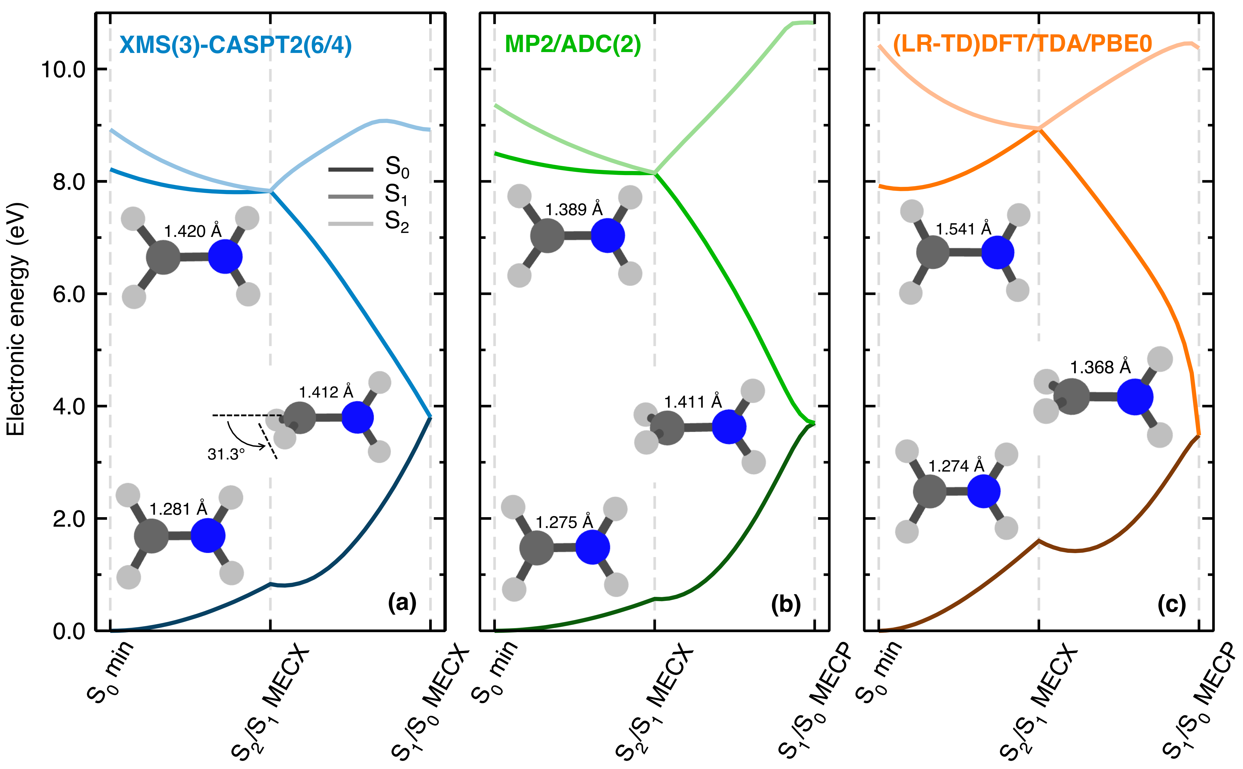
Figure 1: LIIC pathways connecting the S₀ minimum, S₂/S₁ MECX and S₁/S₀ MECX (or MECP) in protonated formaldimine. Comparison of the S₀ (dark colour), S₁ (mid colour) and S₂ (light colour) electronic energies obtained with (a) XMS(3)-CASPT2(6/4)/cc-pVTZ (blue), (b) MP2/ADC(2)/cc-pVTZ (green) and (c) (LR-TD)DFT/TDA/PBE0/cc-pVDZ (orange). In each panel, the critical geometries were optimised at the same level of theory used to compute the electronic energies. The insets show the molecular structures of the three critical points (S₀ min, bottom left; S₂/S₁ MECX, top left; S₁/S₀ MECX (or MECP), middle right) along with the calculated C-N bond lengths (and the CH₂ pyramidalisation angle for the XMS(3)-CASPT2(6/4) S₁/S₀ MECX geometry).

According to XMS-CASPT2 (Fig. 1a), following photoexcitation to S₂, protonated formaldimine decays to S₁ via a strongly peaked S₂/S₁ MECX, which is encountered by a stretch of the C-N bond whilst retaining the planarity of the molecule exhibited at the FC geometry (S₀ min, 1.281 Å; S₂/S₁ MECX, 1.420 Å). Such a peaked topography is assumed to provide highly efficient nonadiabatic population transfer from S₂ to S₁.barbatti_ultrafast_2006 Subsequent relaxation to the ground electronic state occurs through a weakly sloped S₁/S₀ MECX, which for XMS-CASPT2 is reached via a 90^∘ twist of the C-N bond and an additional 31.3^∘ pyramidalisation of the CH₂ moiety. Less efficient S₁-to-S₀ decay is expected for the predicted sloped topography of the S₁/S₀ MECX.barbatti_ultrafast_2006 Previous investigations with MRCISD have reported purely twisted S₁/S₀ MECX geometries with no CH₂ pyramidalisation,levine_optimizing_2008; nikiforov_assessment_2014 whereas others employing MS-CASPT2 have instead predicted the C-N torsion accompanied by pyramidalisation of the NH₂ group.levine_optimizing_2008 The differences in S₁/S₀ MECX geometry obtained by different multireference methods have been ascribed to an apparent flatness of the intersection seam with respect to pyramidalisation (at either end of the C-N bond).levine_optimizing_2008

We now compare the XMS-CASPT2 LIIC pathway to those obtained with (LR-TD)DFT/TDA/PBE0 (Fig. 1c) and MP2/ADC(2) (Fig. 1b). Considering the overall electronic energy profiles of the different methods along the LIIC, an obvious observation is the striking agreement between MP2/ADC(2) and XMS-CASPT2; the only notable difference is the behaviour of S₂ in the segment connecting the two MECXs (explained by the involvement of other electronic states not included in XMS-CASPT2). On the other hand, LR-TDDFT/TDA/PBE0 predicts an ${\rm S}_{2}-{\rm S}_{1}$ energy difference at the S₀ minimum over twice that given by either ADC(2) or XMS-CASPT2. The approach to the respective MECX (or MECP) points are also markedly different in (LR-TD)DFT/TDA/PBE0 compared to that in the wavefunction-based methods. Notably, the LR-TDDFT/TDA/PBE0 S₁ state approaches the S₁/S₀ MECP too steeply relative to XMS-CASPT2. This observation further corroborates that the LR-TDDFT/TDA first excited electronic state can vary too rapidly in the vicinity of a CX with the ground state, as previously shown in Ref. levine_conical_2006. Interestingly, neither MP2/ADC(2) nor (LR-TD)DFT/TDA/PBE0 predict the CH₂ pyramidalisation exhibited by XMS-CASPT2 for the S₁/S₀ MECX geometry, despite all three geometries being at approximately the same relative energy. Earlier works using (LR-TD)DFT/TDA/PBE presented similar observations.tavernelli_non-adiabatic_2009

III.1.2 S₂/S₁ branching space

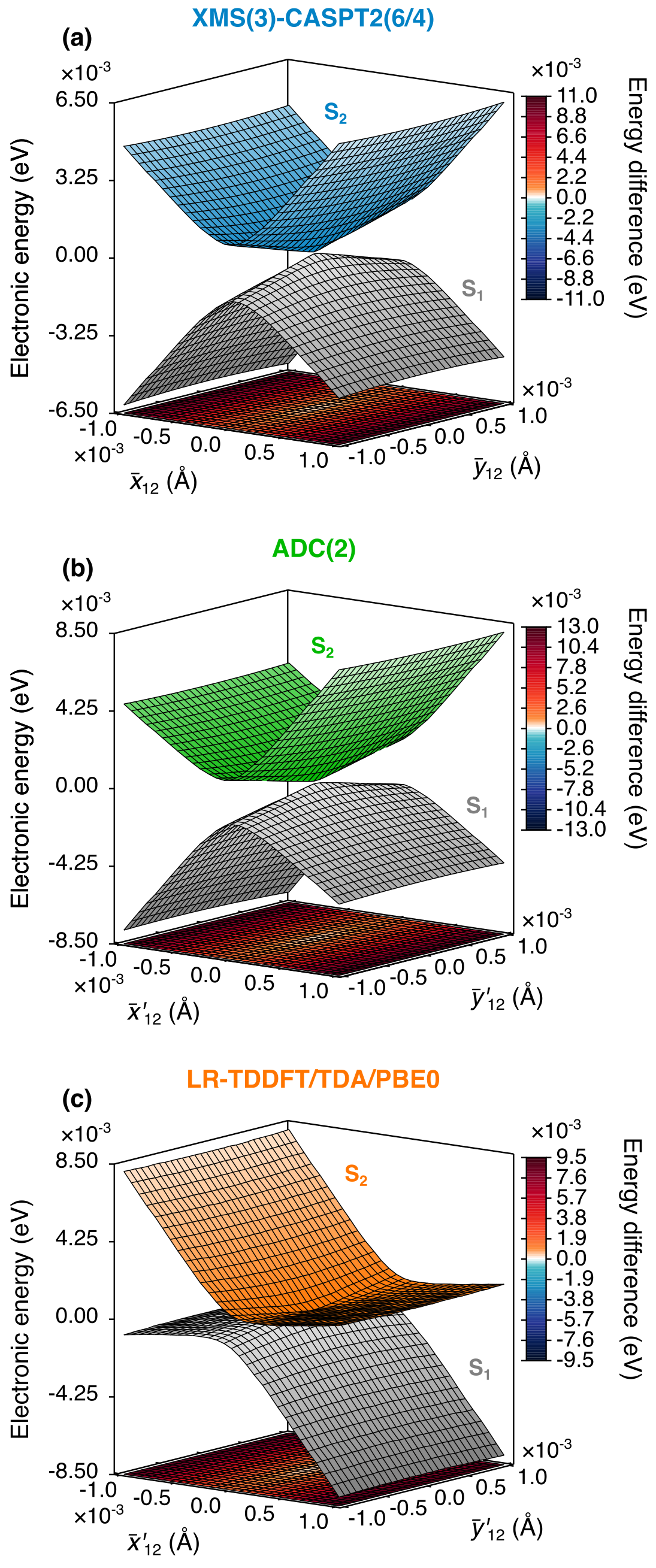
Figure 2: Branching space of the S₂/S₁ MECX in protonated formaldimine. Comparison of the S₁ and S₂ PESs obtained with (a) XMS(3)-CASPT2(6/4)/cc-pVTZ (blue/grey), (b) ADC(2)/cc-pVTZ (green/grey) and (c) LR-TDDFT/TDA/PBE0/cc-pVDZ (orange/grey). In each plot, the MECX geometries and branching space vectors were obtained at the same level of theory used to calculate the electronic energies (except for the ADC(2) plot, which used the $\mathbf{h}_{12}(\mathbf{R})$ vector of XMS(3)-CASPT2(6/4) – see Sec. II.2.3 for details). The base in each plot shows a 2D colour map of the ${\rm S}_{2}-{\rm S}_{1}$ energy difference (see colour bar on the right).

We now focus our attention on the first intersection seam encountered by protonated formaldimine upon photoexcitation to S₂, by calculating the electronic energies with each electronic structure method within the branching space of their respective S₂/S₁ MECX (Fig. 2). All three electronic structure methods correctly predict a conical ($F-2$)-dimensional intersection between S₁ and S₂, where the degeneracy is lifted in both branching space vector directions. We stress again (see Section II.1) that the success of LR-TDDFT/TDA to accurately describe the topology of the S₂/S₁ MECX is not necessarily guaranteed. Our results, however, confirm that linear-response $\mathbf{h}_{12}(\mathbf{R})$ vectors do indeed offer an adequate description of the CX branching space in protonated formaldimine.

We note that the S₁ and S₂ PESs obtained with LR-TDDFT/TDA/PBE0 are in relatively poor agreement with those of the XMS-CASPT2 reference (compare Fig. 2c to Fig. 2a). Using the CX branching space topography parameters defined in Ref. fdez_galvan_analytical_2016, both methods yield a peaked bifurcating topography, but LR-TDDFT/TDA/PBE0 exhibits larger values of $\mathcal{P}$ and $\mathcal{B}$ (0.59 and 0.86, respectively) than XMS-CASPT2 (0.02 and 0.29). These parameters are summarised in the SI. This disparity between LR-TDDFT/TDA/PBE0 and XMS-CASPT2 links to the LIIC plots in Fig. 1, where the approach of the LR-TDDFT/TDA/PBE0 S₂ and S₁ states (i.e., the ${\rm S}_{2}-{\rm S}_{1}$ energy gap and slope of the S₂ and S₁ energies) towards the S₂/S₁ MECX is markedly different in LR-TDDFT/TDA/PBE0 to that in either XMS-CASPT2 or ADC(2). On the other hand, the S₁ and S₂ PESs obtained with ADC(2) are in close agreement with those of XMS-CASPT2; ADC(2) also yields a peaked bifurcating topography for the S₂/S₁ MECX (compare Fig. 2b to Fig. 2a) with similar parameter values of $\mathcal{P}=0.08$ and $\mathcal{B}=0.45$. The ability of ADC(2) to adequately describe the branching space of a CX between excited electronic states is reassuring, given its extended use within excited-state molecular dynamics simulations.plasser_surface_2014; bennett_nonadiabatic_2016; kochman_theoretical_2019; sapunar_timescales_2015; prlj_excited_2015; kochman_simulating_2020; siddique_nonadiabatic_2020; barbatti_photorelaxation_2014; lischka_effect_2018; milovanovic_simulation_2021; prlj_rationalizing_2016; novak_photochemistry_2017; dommett_excited_2017; gate_photodynamics_2019; kochman_theoretical_2016; hutton_photodynamics_2022; szabla_ultrafast_2016

III.1.3 S₁/S₀ branching space

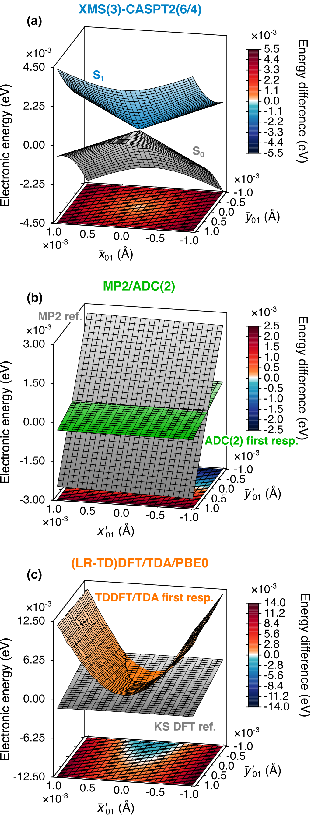
Figure 3: Branching space of the S₁/S₀ MECX (or MECP) in protonated formaldimine. Comparison of the S₀ and S₁ PESs obtained with (a) XMS(3)-CASPT2(6/4)/cc-pVTZ (blue/grey), (b) MP2/ADC(2)/cc-pVTZ (green/grey) and (c) (LR-TD)DFT/TDA/PBE0/cc-pVDZ (orange/grey). In each plot, the MECX (or MECP) geometries and branching space vectors were obtained at the same level of theory used to calculate the electronic energies (except for the MP2/ADC(2) plot, which used the $\mathbf{h}_{01}(\mathbf{R})$ vector of XMS(3)-CASPT2(6/4) – see Sec. II.2.3 for details). The dashed lines in the Figs. 3(b) and 3(c) indicate the seam where $E_{0}(\mathbf{R})=E_{1}(\mathbf{R})$. (We note that the rendering of the colours for the PESs does not reflect precisely this intersection.) The base in each plot shows a 2D colour map of the ${\rm S}_{1}-{\rm S}_{0}$ energy difference (see colour bar on the right).

Next, we take the opportunity to focus on the performance of the methods in describing the S₁/S₀ MECX branching space of protonated formaldimine. XMS-CASPT2 gives a conical ($F-2$)-dimensional intersection as expected (Fig. 3a), with a sloped single-path topography (with parameters, $\mathcal{P}=1.49$ and $\mathcal{B}=1.32$) similar to that reported in Ref. barbatti_ultrafast_2006. As expected from the discussion in Sec. II.1, (LR-TD)DFT/TDA/PBE0 and MP2/ADC(2) incorrectly predict a linear ($F-1$)-dimensional intersection at the S₁/S₀ MECP (Fig. 3c and Fig. 3b, respectively), where the degeneracy is only lifted along a single branching space vector direction (i.e., $\bar{\mathbf{y}}^{\prime}_{01}(\mathbf{R})$). In both cases, the first response (S₁) state becomes lower in energy than the reference (S₀) state, leading to negative excitation energies along certain regions of the branching plane (see colourmap in Fig. 3b and Fig. 3c). This observation corroborates earlier results obtained for (LR-TD)DFTlevine_conical_2006 and MP2/ADC(2).tuna_assessment_2015 When plotted using the same vertical axis energy range (see Fig. S2 in the SI), it is clear that the (LR-TD)DFT/TDA/PBE0 S₁ PES varies too rapidly in the vicinity of the S₁/S₀ MECP compared to that of both XMS-CASPT2 (where a conical intersection is obtained), and MP2/ADC(2) (where a linear seam of intersection is observed). This difference in behaviour between the different electronic structure methods is consistent with the LIIC plots in Fig. 1 close to the S₁/S₀ intersection region. (We note that replacing the (LR-TD)DFT branching space vectors used to generate the (LR-TD)DFT S₁/S₀ MECP (and S₂/S₁ MECX) branching space plots in Fig. 3 (and 2) with those of XMS-CASPT2 results in no observable difference to the PESs – except for a trivial reflection in the $\bar{\mathbf{y}}^{\prime}_{ij}(\mathbf{R})$ vector direction.)

Figure 4: 2D colour map of the electronic energy difference between S₀ (reference state) and S₁ (first response state) obtained with (a) MP2/ADC(2)/cc-pVTZ and (b) (LR-TD)DFT/TDA/PBE0/cc-pVDZ in the vicinity of the S₁/S₀ MECP along an extended branching plane ($\pm 0.003\times\bar{\mathbf{x}}^{\prime}_{01}(\mathbf{R})$, $\pm 0.03\times\bar{\mathbf{y}}^{\prime}_{01}(\mathbf{R})$). The black box encloses the area spanned by the branching plane used to generate the plots in Fig. 3; the black cross indicates the location of the MECP geometry.

Despite indeed being ($F-1$)-dimensional near the point where the two electronic states become degenerate, the (LR-TD)DFT/TDA/PBE0 intersection in Fig. 3c appears significantly more curved than the strictly linear S₁/S₀ intersection of MP2/ADC(2) in Fig. 3b. This observation warrants further investigation of the (LR-TD)DFT/TDA/PBE0 intersection at larger distances along the $\bar{\mathbf{y}}^{\prime}_{01}(\mathbf{R})$ vector direction. Plotting the (LR-TD)DFT/TDA/PBE0 S₀ and S₁ PESs along an extended branching plane ($\pm 0.003\times\bar{\mathbf{x}}^{\prime}_{01}(\mathbf{R})$ and $\pm 0.03\times\bar{\mathbf{y}}^{\prime}_{01}(\mathbf{R})$ in Fig. 4b compared to the original $\pm 0.001\times\bar{\mathbf{x}}^{\prime}_{01}(\mathbf{R})$ and $\pm 0.001\times\bar{\mathbf{y}}^{\prime}_{01}(\mathbf{R})$ in Fig. 3 – see SI for branching space vector definitions) reveals that the curved intersection seam in Fig. 3c is in fact just one part of a larger intersection ring - something that shows a striking resemblance to two interpenetrating cones. On the other hand, the strictly linear intersection seam in MP2/ADC(2) observed along the standard branching plane (Fig. 3b) remains even along this extended branching plane (Fig. 4a). Overall, our results connect the different pictures proposed earlier for the description of S₁/S₀ MECPs within (LR-TD)DFT/TDA: performing an S₁/S₀ MECP optimisation with (LR-TD)DFT/TDA will in fact locate a geometry on the intersection ring and the MECP will look different depending on the extent of the branching space explored to unravel the shape of the S₀ and S₁ PESs around this location – either a (near-to-linear) seam of intersection for minute variations along $\bar{\mathbf{x}}^{\prime}_{01}(\mathbf{R})$ and $\bar{\mathbf{y}}^{\prime}_{01}(\mathbf{R})$ (like in Fig. 3c and as first reported by Levine et al.levine_conical_2006), or an intersection ring (reminiscent of two interpenetrating cones) when a more extended scan along $\bar{\mathbf{x}}^{\prime}_{01}(\mathbf{R})$ and $\bar{\mathbf{y}}^{\prime}_{01}(\mathbf{R})$ is performed (like in Fig. 4b and as alluded to by Tapavicza et al.tapavicza_mixed_2008). We note that it may be possible to miss the negative-energy region of the intersection ring for more extreme scans around the (LR-TD)DFT/TDA S₁/S₀ intersection point (i.e., if one ”zooms out” further from the crossing point), giving a false impression that (LR-TD)DFT/TDA can describe the intersection point adequately.

We conclude this Section by noting that we also calculated the HF/CIS S₁/S₀ MECP branching space for both the standard and extended grid of geometries around the intersection point – see Figs. S4 and S5 in the SI. As expected (Section II.1) HF/CIS predicts a strictly linear ($F-1$)-dimensional intersection along the standard branching plane that likewise remains along the extended branching plane, which is analogous to the behaviour of MP2/ADC(2), but in contrast to that of (LR-TD)DFT/TDA/PBE0. We have confirmed that our (LR-TD)DFT/TDA findings are unaffected by improving the numerical accuracy of our calculations (i.e., increased grid size – see also the SI for details regarding SCF convergence). These observations solidify our conclusions that the description of CXs involving the ground state by (LR-TD)DFT/TDA and HF/CIS are not completely analogous.

III.2 Pyrazine

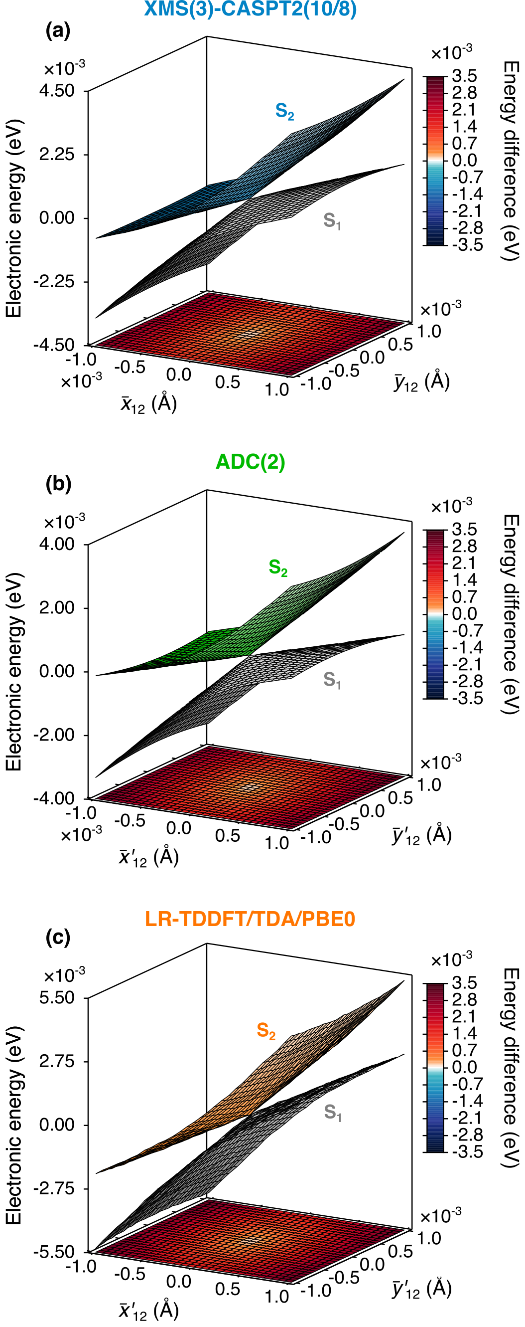
Figure 5: Branching space of the S₂/S₁ MECX in pyrazine. Comparison of the S₁ and S₂ PESs obtained with (a) XMS(3)-CASPT2(6/4)/cc-pVTZ (blue/grey), (b) ADC(2)/cc-pVTZ (green/grey) and (c) LR-TDDFT/TDA/PBE0/cc-pVDZ (orange/grey). In each plot, the MECX geometries and branching space vectors were obtained at the same level of theory used to calculate the electronic energies (except for the ADC(2) plot, which used the $\mathbf{h}_{12}(\mathbf{R})$ vector of XMS-CASPT2(10/8) – see Sec. II.2.3 for details). The base in each plot shows a 2D colour map of the ${\rm S}_{2}-{\rm S}_{1}$ energy difference (see colour bar on the right).

Next, we consider CXs between excited states for a second exemplar molecule, pyrazine. Like for protonated formaldimine, the excited electronic states of pyrazine have been well-studied, often considered the definitive case for vibronic coupling in aromatic systems; pyrazine is also a precursor to numerous biologically active molecules.woywod_theoretical_2010; stock_resonance_1995; sala_quantum_2015; shiozaki_pyrazine_2013; woywod_characterization_1994; kanno_ab_2015; sobolewski_ab_1993; seidner__1992 Within the FC region, the S₁ state in pyrazine exhibits an $n\pi^{*}$ character and S₂ is of $\pi\pi^{*}$ character.woywod_characterization_1994 At the XMS-CASPT2 level, the S₂/S₁ MECX is reached (from the planar S₀ minimum geometry) by simultaneous elongation of the C-N and C-C bonds, but with an overall stretching of the ring along the axis bisecting the two nitrogen atoms (see Fig. S6 in the SI). LR-TDDFT/TDA/PBE0 and ADC(2) predict S₀ minimum and S₂/S₁ MECX geometries that agree closely with those of XMS-CASPT2. The only difference is the stretching of the S₂/S₁ MECX geometry observed in LR-TDDFT/TDA/PBE0 is slightly more exaggerated than in the wavefunction-based methods, as indicated by the larger (smaller) N-C-C (C-N-C) bond angles. This distortion in the LR-TDDFT/TDA/PBE0 S₂/S₁ MECX geometries is accompanied by it being approximately 1 eV higher in energy than the S₂/S₁ MECX geometry in either XMS-CASPT2 or ADC(2).

III.2.1 S₂/S₁ branching space

We focus on the respective branching spaces for the S₂/S₁ MECX (Fig. 5). As for protonated formaldimine, all three methods correctly predict a conical ($F-2$)-dimensional intersection between S₁ and S₂, where the degeneracy is lifted along both branching space vector directions. LR-TDDFT/TDA/PBE0 exhibits a sloped single-path MECX, mirroring the topography observed with both XMS-CASPT2 and ADC(2), with $\mathcal{P}$ and $\mathcal{B}$ parameters (7.16 and 2.64, respectively) that are closer to those obtained with XMS-CASPT2 (3.57 and 1.96) than ADC(2) (12.78 and 1.14). Recalculating the S₂/S₁ MECX geometry and its corresponding branching space with a different exchange-correlation functional (i.e., the range-separated hybrid LC-$\omega$PBE, with range-separated parameter $\omega$ = 0.4 $a_{0}^{-1}$ – see Fig. S7 in the SI) further generalises our findings and conclusions that LR-TDDFT/TDA can adequately reproduce the dimensionality of a CX between excited electronic states.

IV Conclusion

This work has shown explicitly that LR-TDDFT/TDA/PBE0 within the AA is able to exhibit the correct topology of a CX between two excited electronic states for two exemplar molecules, protonated formaldimine and pyrazine. The correct CX topology was unchanged when an alternative exchange-correlation functional was investigated for pyrazine. We further showed that ADC(2) offers an accurate description of both the topology and topography of CXs between excited electronic states, and note that this is in contrast to that of (conventional) coupled cluster theory, which can be flawed in this context.plasser_surface_2014; hattig_structure_2005; kohn_can_2007; kjonstad_crossing_2017; thomas_complex_2021 We stress that all CX branching spaces analysed in this work were constructed within a fully-consistent approach where all required electronic quantities were computed (where possible) at the same level of theory.

Re-inspection of the problem faced by AA (LR-TD)DFT/TDA to adequately describe CXs involving the ground electronic states also proved fruitful. Our findings for protontated formaldimine show that the two, supposedly different, pictures related to the S₁/S₀ MECP branching space of AA (LR-TD)DFT/TDA/PBE0 – a seam of intersection vs. two interpenetrating cones – both emanate from the intersection ring, which can be reconciled by analysing the behaviour of the PESs, either in the immediate vicinity of the S₁/S₀ MECP, or at further distances from the MECP geometry. The intersection ring from AA (LR-TD)DFT/TDA/PBE0 is in stark contrast to the linear intersection observed from MP2/ADC(2) (and, as expected, HF/CIS). Further work is arguably still needed to pinpoint precisely how nonadiabatic dynamics simulations is influenced by the intersection ring and whether the difference in behaviour of AA (LR-TD)DFT/TDA/PBE0 to that of HF/CIS gives any grounds for optimism when applying AA (LR-TD)DFT/TDA in this context. Again, extending the use of previously proposed expressions for the exact, frequency-dependent exchange-correlation kernelmaitra_double_2004; casida_propagator_2005; ferre_many-body_2015; romaniello_double_2009; gritsenko_double_2009; strinati_application_1988; zhang_dynamical_2013; authier_dynamical_2020; thiele_frequency_2014 to the problem of CXs involving the ground electronic state still remains as pertinent as ever. Nonetheless, for the case of CXs between excited electronic states, greater confidence (at least for electronic states dominated by single excitations) should be felt when applying AA LR-TDDFT/TDA to chemically (and biologically) relevant systems, whose size still prohibits the use of multiconfigurational methods.

Data availability

The data that supports the findings of this study are available within the article and its supplementary material.