Calibrating baryonic feedback with weak lensing and fast radio bursts

Abstract

One of the key limitations of large-scale structure surveys of the current and future generation, such as Euclid, LSST-Rubin or Roman, is the influence of feedback processes on the distribution of matter in the Universe. This effect, called baryonic feedback, modifies the matter power spectrum on non-linear scales much stronger than any cosmological parameter of interest. Constraining these modifications is therefore key to unlock the full potential of the upcoming surveys, and we propose to do so with the help of Fast Radio Bursts (FRBs). FRBs are short, astrophysical radio transients of extragalactic origin. Their burst signal is dispersed by the free electrons in the large-scale-structure, leading to delayed arrival times at different frequencies characterised by the dispersion measure (DM). Since the dispersion measure is sensitive to the integrated line-of-sight electron density, it is a direct probe of the baryonic content of the Universe. We investigate how FRBs can break the degeneracies between cosmological and feedback parameters by correlating the observed Dispersion Measure with the weak gravitational lensing signal of a Euclid-like survey. In particular we use a simple one-parameter model controlling baryonic feedback, but we expect similar findings for more complex models. Within this model we find that $\sim 10^{4}$ FRBs are sufficient to constrain the baryonic feedback 10 times better than cosmic shear alone. Breaking this degeneracy will tighten the constraints considerably, for example we expect a factor of two improvement on the sum of neutrino masses.

1 Introduction

Cosmic shear, the weak gravitational lensing effect imprinted on distant galaxies by the large-scale structure (LSS), is one of the primary science goals for the the upcoming stage-4 surveys Euclid, Rubin-LSST and the Roman telescope. The foundations for these missions has been laid down by their predecessors: the Kilo-Degree Survey [1, 2, KiDS], the Dark Energy Survey [3, 4, DES] and the Subaru Hyper Suprime-Cam [5, 6, HSC].

The stage-4 surveys in particular target the highly non-linear regime of the matter distribution. Even though there is a wealth of information to be gathered at $k>1\,\mathrm{Mpc}^{-1}h$, baryonic feedback (BF) processes imprint large theoretical uncertainties on the total matter power spectrum. While the distribution of collisionless cold dark matter is well understood, at least on the level of numerical simulations, baryons remain the cause of large uncertainties. The displacement of baryons is due to nonlinear effects sourced by star formation, Supernovae, Active Galactic Nuclei (AGN) or cooling [see e.g. 7, 8, for reviews]. In turn, the displaced baryons affect the total matter power spectrum causing a reduction of power on intermediate scales due to outflows and energy injection by e.g. AGN, and an increase in power on small scales due to cooling. As these effects span a multitude of scales and are highly non-linear, they are almost impossible to model analytically and are thus extracted from hydrodynamical simulations which include a model with a fixed set of parameters to control the feedback strength. The main challenge arises from the fact that feedback processes originate from physics which is far below the resolution of the numerical simulation. Each simulation therefore has sub-grid models implemented. However, different models can lead to significantly different predictions for the matter clustering statistics at small scales [9, 10]. For example, in the CAMELS simulation suite [11] two very distinct sub-grid models are implemented. However, the differences are largely due to higher gas temperature in the inter-galactic medium [11]. Another suite of simulations are the BAHAMAS simulations [12] whose power spectra have been calibrated to a hydrodynamical version of the halo model [13], specifically designed for weak lensing cross correlations studies with the thermal Sunyae-Zel’dovich (tSZ) effect [14].

Any independent measurement of the baryon distribution can help to independently constrain feedback models. It was shown in [14] that e.g. the tSZ effect has the potential to partially calibrate the feedback strength and breaking degeneracies (see also a discussion [15]). At the moment, the tSZ effect is the only way to measure the electron distribution in the Universe. It is therefore important to add additional probes for $(i)$ more constraining power and $(ii)$ different systematic effects in the measurements.

An alternative probe of the electron distribution are fast radio bursts (FRBs). FRBs are short transients, lasting typically a few milliseconds, with frequencies ranging from $\sim 100$ MHz to several GHz. Since the radio signal is travelling through the ionized intergalactic medium (IGM), each frequency of the pulse experiences a delay characterised by the dispersion measure (DM) proportional to the integrated free electron density along the line-of-sight [e.g. 16, 17, 18, 19, 20]. The mechanism responsible for the radio emission is currently unknown, but the isotropic occurrence of the events detected so far shows no alignment with the Milky Way disk and the measured DM for most events is very large, requiring an extragalactic origin. By now, a subset of events has been localised to galaxies up to redshifts $z\sim 1$. In general, the total DM associated with an extragalactic FRB event consists of contributions from the host galaxy, the Milky Way and the diffuse electrons in the large-scale structure (LSS). Several authors therefore proposed to use the DM inferred from FRBs as a cosmological probe using either the averaged signal [e.g. 21, 22, 23, 24, 25, 26, 27, 28] or the statistics of DM fluctuations [e.g. 29, 30, 31, 32, 33, 34, 35].

Currently roughly $\sim 800$ FRBs are detected, but estimated rates of $\sim 1000$ events/night/sky allow surveys such as CHIME, UTMOST, HIRAX, ASKAP or SKA [36, 37, 38, 39] to provide at least $\sim 10^{4}$ FRBs per decade. Although FRBs do not show spectral features that allow for accurate redshift estimation, the accumulated DM can be translated into a noisy distance estimate [29]. Since FRBs are observed with $\mathrm{DM}\geq 1000\;\mathrm{pc}\;\mathrm{cm}^{-3}$ and models of the Milky way suggest $\mathrm{DM}\leq 50\;\mathrm{pc}\;\mathrm{cm}^{-3}$ due to gas in our Galaxy for most directions on the sky [40], the majority of the DM signal originates from the diffuse electrons in the IGM, which follows the total matter distribution on large scales. Although the host galaxy contribution is still under debate, its magnitude is expected to be comparable to that of the Milky Way and hence usually smaller than the contribution from the LSS. While the host dispersion can reach several hundreds $\mathrm{pc}\;\mathrm{cm}^{-3}$ in rare cases, particularly when the FRB is originates in the trailing edge of the host galaxy (as seen by the observer), one typically finds that $\mathrm{DM}_{\mathrm{LSS}}>\mathrm{DM}_{\mathrm{host}}$ for FRBs at redshifts $z\sim 1$. The dispersion of FRBs tests, similar to cosmic shear, an integrated quantity along the line-of-sight. However, since host galaxies typically contribute less to the DM than the LSS, FRBs are way less affected by shot noise compared to cosmic shear. Combining FRBs and cosmic shear will accordingly probe similar structures, but testing the baryon distribution and the total matter distribution respectively, enabling strong constraints on the different clustering behaviour of both components. It should be noted that the cosmic shear signal has a vanishing expectation value, unlike the DM of FRBs. However, since we are interested in the statistical properties of the DM this is not that important for our study here.

In this paper we will hence investigate the potential gains from combining a stage-4 cosmic shear measurement with the statistical properties of the DM measured from an FRB sample which should be available on the same timescale as cosmic shear data from Euclid and Rubin-LSST. To this end, we simulate mock data for these kind of surveys and carry out a Fisher and MCMC analysis to investigate the impact of adding FRBs in a cosmological analysis with a particular focus on the baryonic feedback and on the cosmological parameters that are most affected by feedback uncertainties, such as the sum of neutrino masses. The paper is structured as follows: In Section 2 we summarise the LSS structure probes and describe the methodology for our analysis. Section 3 is devoted to the discussion of the results and a comparison with other probes of the electron distribution. Lastly, we conclude in Section 4 and discuss potential ways forward.

2 Large-Scale-Structure Probes

In this section we summarise the two probes used to test the matter distribution: cosmic shear and FRB dispersion measure. We introduce cosmic shear in Section 2.1 and DM correlations in Section 2.2, which are sensitive to the full matter and electron distribution respectively and can hence be used to break degeneracies between baryonic feedback and cosmological parameters.

2.1 Cosmic Shear

Cosmic shear is the gravitational lensing effect of the LSS on an ensemble of background sources (galaxies) and is thus sensitive to the projected matter distribution along the line-of-sight. The cosmological information of gravitational lensing by the LSS is contained in the traceless part of the cosmic shear tensor:

$$\boldsymbol{\gamma}_{i}=2\int\mathrm{d}\chi W_{\gamma_{i}}(\chi)\eth\eth\Phi(\hat{\boldsymbol{x}},\chi)\;,$$ (2.1)

in absence of anisotropic stress. Here $\gamma_{i}$ denotes the shear in the $i$-th tomographic bin, $W_{\gamma_{i}}$ is a geometrical weighting function defined below, $\Phi$ are the scalar metric perturbations, $\chi$ the co-moving distance and $\eth$ is the eth-derivative for a spin-2 field. Using Poisson’s equation, one can relate the metric perturbations to the density contrast, yielding the following expression for the angular power spectrum:

$$C^{\gamma_{i}\gamma_{j}}_{\ell}=\frac{(\ell+2)!}{(\ell-2)!}\frac{2}{\uppi}\int\mathrm{d}\chi_{1}\int\mathrm{d}\chi_{2}\int k^{2}\mathrm{d}k\;K_{i}(\chi_{1})K_{j}(\chi_{2})\frac{j_{\ell}(\chi_{1}k)}{(k\chi_{1})^{2}}\frac{j_{\ell}(\chi_{2}k)}{(k\chi_{2})^{2}}\sqrt{P_{\delta}(k,\chi_{1})P_{\delta}(k,\chi_{2})}\;.$$ (2.2)

Approximating the Bessel function by a Dirac distribution [41, 42], the integrations over $\chi_{1,2}$ can be carried out to find the commonly used expression for for the angular power spectrum:

$$C^{\gamma_{i}\gamma_{j}}_{\ell}=\int_{0}^{\chi_{\mathrm{H}}}\frac{\mathrm{d}\chi}{\chi^{2}}W^{(i)}_{\gamma}(\chi)W^{(j)}_{\gamma}(\chi)P_{\delta}\left(\frac{\ell+1/2}{\chi},\chi\right)\;,$$ (2.3)

which will be accurate enough for cosmic shear even for the next generation of surveys [43] due to the broad lensing kernel. Here $P_{\delta}$ is the matter power spectrum, for which we use the emulated spectrum from HMcode[44]. $W^{(i)}_{\gamma}(\chi)$ is the lensing weight of the $i$-th tomographic bin as given by:

$$W^{(i)}_{\gamma}(\chi)=\frac{3\Omega_{\mathrm{m0}}}{2\chi_{\mathrm{H}}^{2}}\frac{\chi}{a(\chi)}\int_{\chi}^{\chi_{\mathrm{H}}}\mathrm{d}{\chi^{\prime}}n^{(i)}_{\mathrm{s}}({\chi^{\prime}})\frac{{\chi^{\prime}}-\chi}{{\chi^{\prime}}}\;.$$ (2.4)

Here $a$ is the scale factor, $\Omega_{\mathrm{m}0}$ the matter density parameter today, $\chi_{\mathrm{H}}$ the Hubble radius and $n^{(i)}_{\mathrm{s}}$ is the distribution of sources.

Lastly, due to the finite number of background galaxies, observed spectra obtain a shape-noise contribution:

$$C^{\gamma_{i}\gamma_{j}}_{\ell}\;\to\;C^{\gamma_{i}\gamma_{j}}_{\ell}+\frac{\sigma_{\epsilon,i}^{2}}{2\bar{n}_{i}}\;,$$ (2.5)

with the total ellipticity dispersion $\sigma_{\epsilon,i}^{2}$ and the average number of sources $\bar{n}_{i}$ in the $i$-th tomographic bin.

Survey	area $f_{\mathrm{sky}}$	number of sources	intrinsic noise $\sigma$	tomographic bins
FRB	0.7	$10^{4}$	$50\;\mathrm{pc}\;\mathrm{cm}^{-3}$	1
Euclid	0.3	$30\;\mathrm{arcmin}^{-2}$	0.3	10
KiDS	0.025	$7.55\;\mathrm{arcmin}^{-2}$	0.28	5

Table 1: Survey settings assumed in the analysis. The number of sources for the cosmic shear surveys is an average density over all tomographic bins. The actual number in each tomographic bin can be slightly different. The same holds for the ellipticity dispersion, for more details see [45] and [46].

2.2 FRB statistics

FRB pulses undergo dispersion while travelling through the ionized IGM, causing a frequency-dependent (proportional to $\nu^{-2}$) offset of arrival times. The corresponding time delay measured $\delta t(\hat{\boldsymbol{x}},z)$ for an FRB at redshift $z$ in direction $\hat{\boldsymbol{x}}$ proportional to the observed dispersion measure: $\delta t(\hat{\boldsymbol{x}},z)=\mathrm{DM}_{\mathrm{tot}}(\hat{\boldsymbol{x}},z)\nu^{-2}$. The observed DM can be broken up into different components:

$$\mathrm{DM}_{\mathrm{tot}}(\hat{\boldsymbol{x}},z)=\mathrm{DM}_{\mathrm{LSS}}(\hat{\boldsymbol{x}},z)+\mathrm{DM}_{\mathrm{MW}}(\hat{\boldsymbol{x}})+\mathrm{DM}_{\mathrm{host}}(z)\;,$$ (2.6)

where $\mathrm{DM}_{\mathrm{LSS}}(\hat{\boldsymbol{x}},z)$ is the DM caused by the electron distribution in the LSS, while $\mathrm{DM}_{\mathrm{MW}}(\hat{\boldsymbol{x}})$ and $\mathrm{DM}_{\mathrm{host}}(z)$ describe the contributions from the Milky Way and the host galaxy, respectively. Here we made the dependence on redshift and direction explicit. Note that the rest-frame DM of the host, $\mathrm{DM}_{\mathrm{host,rf}}$, is observed as $\mathrm{DM}_{\mathrm{host}}(z)=(1+z)^{-1}\mathrm{DM}_{\mathrm{host,rf}}$.

Current models of the galactic electron distribution predict ${\mathrm{DM}_{\mathrm{MW}}\sim 60\,\mathrm{pc}\,\mathrm{cm}^{-3}}$ over most of the sky [40, 47]. Since the galactic electron distribution also depends on the direction $\hat{\boldsymbol{x}}$, it is in principle a large contaminant for DM correlation measurement. Here, however, we assume that it can be modelled accurately enough to be subtracted from the observed DM without leaving a significant imprint on the measured DM correlations. Naively one can expect $\mathrm{DM}_{\mathrm{host}}(z)$ to be very similar to $\mathrm{DM}_{\mathrm{MW}}$. However, in practice it depends strongly on the host galaxy’s properties and is thus treated as a free parameter. Since it does not correlate with the LSS, it will not leave an imprint on the DM correlation but rather act as a noise term as we will discuss later. Finally, the LSS contribution to the DM is given by [34]

$$\mathrm{DM}_{\mathrm{LSS}}(\hat{\boldsymbol{x}},z)=\chi_{\mathrm{H}}\int_{0}^{z}\mathrm{d}z^{\prime}\,n_{\mathrm{e}}({\boldsymbol{x}},z^{\prime})\,\frac{1+z^{\prime}}{E(z^{\prime})}\,\;,$$ (2.7)

where $E(z)$ is the expansion function and $n_{e}$ the electron density which depends on the local matter over-density, $\delta_{\mathrm{m}}(\boldsymbol{x},z)$ and the electron bias $b_{\mathrm{e}}({\boldsymbol{x}},z)$:

$$n_{\mathrm{e}}({\boldsymbol{x}},z)=\frac{\bar{\rho}_{\mathrm{b}}(z)}{m_{\mathrm{p}}}F(z)\left[1+b_{\mathrm{e}}({\boldsymbol{x}},z)\,\delta_{\mathrm{m}}({\boldsymbol{x}},z)\right]\;.$$ (2.8)

Here we used the mean baryon density $\bar{\rho}_{\mathrm{b}}(z)$, the proton mass $m_{\mathrm{p}}$ and the mass fraction $F(z)$ of electrons in the IGM. The latter can be expressed as:

$$F(z)=f_{\mathrm{IGM}}(z)[Y_{\mathrm{H}}X_{\mathrm{e},\mathrm{H}}(z)+Y_{\mathrm{He}}X_{\mathrm{e},\mathrm{He}}(z)]\;,$$ (2.9)

with the mass fraction of hydrogen and helium $Y_{\mathrm{H}}=0.75$ and $Y_{\mathrm{He}}=0.25$ respectively, as well as their ionization fractions $X_{\mathrm{e},\mathrm{H}}(z)$ and $X_{\mathrm{e},\mathrm{He}}(z)$. Since both hydrogen and helium are both fully ionised for $z\lower 2.15277pt\hbox{$\;\buildrel<\over{\sim}\;$}3$ [48, 49] we set $X_{\mathrm{e},\mathrm{H}}=X_{\mathrm{e},\mathrm{He}}=1$. It should be noted that for the survey settings considered here the majority of the signal arises from $z<3$, so the last assumption is indeed well justified. The fraction of baryons in the IGM, $f_{\mathrm{IGM}}(z)$, has a slight redshift dependence [50], with $10\%\;(20\%)$ locked up in galaxies at $z\lower 2.15277pt\hbox{$\;\buildrel>\over{\sim}\;$}1.5\;(\lower 2.15277pt\hbox{$\;\buildrel<\over{\sim}\;$}0.4)$. Rewriting eq. 2.7 leaves us with the following expression:

$$\!\!\mathrm{DM}_{\mathrm{LSS}}(\hat{\boldsymbol{x}},z)=\mathcal{A}\!\int_{0}^{z}\!\!\!\mathrm{d}z^{\prime}\frac{1+z^{\prime}}{E(z^{\prime})}F(z^{\prime})[1\!+\!b_{\mathrm{e}}({\boldsymbol{x}},z^{\prime})\delta_{\mathrm{m}}({\boldsymbol{x}},z^{\prime})]\;,$$ (2.10)

with the amplitude

$$\mathcal{A}\equiv\frac{3H_{0}^{2}\Omega_{\mathrm{b}0}\chi_{H}}{8\uppi Gm_{\mathrm{p}}}\;.$$ (2.11)

A very intriguing aspect of FRBs is that the cosmological contribution is typically larger than the contribution from the host or the Milky Way. This is in large contrast to cosmic shear, where the ellipticity imprinted by gravitational lensing is a percent effect of the intrinsic ellipticity. Therefore, far fewer FRBs are required for a significant detection of DM correlations compared the number of galaxies in weak lensing studies. Following [34], we rewrite the LSS contribution to the DM as a background contribution and a perturbation:

$$\mathrm{DM}_{\mathrm{LSS}}(\hat{\boldsymbol{x}},z)=\langle\mathrm{DM}_{\mathrm{LSS}}\rangle(z)(1+\mathcal{D}(\hat{\boldsymbol{x}},z))\;,$$ (2.12)

where $\mathcal{D}(\hat{\boldsymbol{x}},z)$ is the effective DM induced by the fluctuations in the LSS. In full analogy to cosmic shear, we assume a source-redshift distribution $n_{\mathrm{FRB}}(z)$. To be accurate, one is using a source-DM distribution, which in turn is converted to $n_{\mathrm{FRB}}(z(\mathrm{DM}))$. This procedure was discussed in [34] and [51]. Note that we do not make use of the fraction of FRBs that will most likely have an identified host with redshift estimates, which additionally improves the expected constraints. By rearranging integration limits one finds

$$\mathcal{D}(\hat{\boldsymbol{x}})=\int_{0}^{\chi_{H}}\!\!\mathrm{d}\chi\;W_{\mathcal{D}}(\chi)\delta_{\mathrm{e}}\big{(}\hat{\boldsymbol{x}},z(\chi)\big{)}\;,$$ (2.13)

with the averaged weighting function

$$W_{\mathcal{D}}(\chi)=W(\chi)\int_{\chi}^{\chi_{H}}\mathrm{d}\chi^{\prime}n_{\mathrm{FRB}}(\chi^{\prime})\;,$$ (2.14)

and $W(\chi)$ being defined via eq. 2.10:

$$W(\chi)=\mathcal{A}\frac{F\big{(}z(\chi)\big{)}\big{(}1+z(\chi)\big{)}}{E\big{(}z(\chi)\big{)}}\left|\frac{\mathrm{d}z}{\mathrm{d}\chi}\right|\;.$$ (2.15)

In complete analogy to cosmic shear, the angular power spectrum for the DM fluctuations $\mathcal{D}$ is given by:

$$C^{\mathcal{D}\mathcal{D}}(\ell)=\;\frac{2}{\uppi}\int\mathrm{d}\chi_{1}\int\mathrm{d}\chi_{2}\int k^{2}\mathrm{d}k\;W_{\mathcal{D}}(\chi_{1})W_{\mathcal{D}}(\chi_{2})\sqrt{P_{\mathrm{ee}}(k,\chi_{1})P_{\mathrm{ee}}(k,\chi_{2})}j_{\ell}(k\chi_{1})j_{\ell}(k\chi_{2})\;.$$ (2.16)

As discussed in [34], the Limber approximation is suitable for DM correlations as well. Hence, we again use eq. 2.3. When cross-correlating cosmic shear and the DM, we replace one of the weight functions in Equation 2.3 with $W_{\mathcal{D}}$ and the matter power spectrum by the electron-matter cross power spectrum $P_{\delta\mathrm{e}}$.

Lastly, the host galaxy contribution acts as a shot noise contribution with variance $\sigma^{2}_{\mathrm{host}}$ per event, thus adding a white noise contribution to the observed spectra:

$$C^{\mathcal{D}\mathcal{D}}(\ell)\;\to\;C^{\mathcal{D}\mathcal{D}}(\ell)+\frac{\sigma^{2}_{\mathrm{host}}}{\bar{n}}\;.$$ (2.17)

2.3 Power Spectra

The angular power spectra in Equation 2.2 and Equation 2.16 are integrals over the matter power spectrum and the electron power spectrum. Cross-correlating the probes also requires the matter-electron power spectrum. We use pyhmcode [44, 13, 14] which was fitted to the BAHAMAS [12] and COSMO-OWLS [52] simulation suites to reproduce the power spectra of matter, gas, stars and pressure assuming a halo model. The baryonic feedback in pyhmcode is controlled by a single parameter, the strength of AGN encapsulated in $T_{\mathrm{AGN}}$. This AGN temperature should just be seen as a nuisance parameters without physical correspondence in the real Universe. Larger AGN temperatures lead to different suppression on large $k$ (and rise again on even smaller scales). For current cosmological surveys, this description is usually flexible enough, since more extended models are likely to be prior dominated and therefore offer too much flexibility. For future surveys, however, more flexible emulators might be needed [53, 54, 55], allowing for more freedom at non-linear scales due to baryonic feedback.

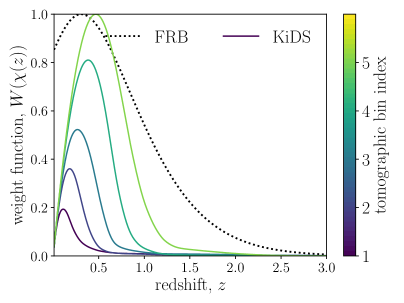
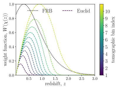
Figure 1: Weighting function for FRBs (dotted black line) and for cosmic shear with the KiDS redshift distribution (left plot) or Euclid’s redshift distribution (right plot). The colour bar shows the tomographic bin index. All weighting functions have been normalised to the peak value. In the case of cosmic shear the peak of the last tomographic bin was used.

2.4 Statistics

Full sky surveys measure $2\ell+1$ independent modes per multipole $\ell$. For any projected fields $f_{i}(\hat{\boldsymbol{x}})$, one would derive modes $f_{i,\ell m}$ from a spherical harmonic decomposition. Assuming that the likelihood for the set of modes $\{f_{i,\ell m}\}$ is a multivariate Gaussian with zero mean and covariance (or 2-point correlation) $\boldsymbol{C}$ with components

$$(\boldsymbol{C}_{\ell})_{ij}=\langle f_{i,\ell m}f^{*}_{j,\ell^{\prime}m^{\prime}}\rangle\equiv\delta^{\mathrm{K}}_{mm^{\prime}}\delta^{\mathrm{K}}_{\ell\ell^{\prime}}C^{f_{i}f_{j}}_{\ell}\;,$$ (2.18)

the Fisher matrix is given by [56]:

$$F_{\alpha\beta}=f_{\mathrm{sky}}\sum_{\ell}\frac{2\ell+1}{2}\mathrm{tr}\left(\boldsymbol{C}^{-1}_{\ell}\partial_{\alpha}\boldsymbol{C}_{\ell}\boldsymbol{C}^{-1}_{\ell}\partial_{\beta}\boldsymbol{C}_{\ell}\right)\;.$$ (2.19)

Here greek indices label parameters, and the observed sky fraction $f_{\mathrm{sky}}$ accounts for incomplete sky coverage. The inverse of the Fisher matrix $\boldsymbol{F}^{-1}$ yields the covariance matrix of the parameters and serves as a lower limit for obtainable errors given the survey settings by means of the Cramér-Rao bound.

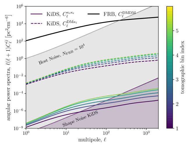
Figure 2: Angular power spectra for the KiDS redshift distributions and an FRB sample with $\alpha=3.5$ as defined in Equation 3.1. The solid black line shows the auto-correlation spectrum of the DM, while the solid lines from blue to yellow depict the cosmic shear power spectrum for the five tomographic bins of KiDS. Dashed lines show the cross-correlation between the DM and cosmic shear. The shaded areas indicate the noise contribution, ignoring sample variance, for both measurements. Note that the noise can vary slightly across the tomographic bins for KiDS.

Since the derivative in eq. 2.19 is calculated numerically, small difference can propagate into the matrix inversion to obtain possible constraints. Therefore, we check the stability of the derivative in appendix A. Lastly, we are also calculating the signal-to-noise ratio (SNR) of the measurement, i.e. we assume that one wants to measure the amplitude, $A$, of the cosmological term in eqs. 2.5 and 2.17. Using eq. 2.19 for $\boldsymbol{C}=A\boldsymbol{S}+\boldsymbol{N}$, one finds

$$\Sigma^{2}(\leq\ell)=f_{\mathrm{sky}}\sum_{\ell^{\prime}}^{\ell}\frac{2\ell^{\prime}+1}{2}\mathrm{tr}\left(\boldsymbol{C}^{-1}_{\ell^{\prime}}\boldsymbol{S}_{\ell^{\prime}}\boldsymbol{C}^{-1}_{\ell^{\prime}}\boldsymbol{S}_{\ell^{\prime}}\right)\equiv\sum_{\ell^{\prime}}^{\ell}\mathcal{S}^{2}(\ell^{\prime})\;.$$ (2.20)

In the case here, the covariance takes the form:

$$\boldsymbol{C}_{\ell}=\begin{pmatrix}\boldsymbol{C}^{\mathcal{D}\mathcal{D}}_{\ell}&\boldsymbol{C}^{\mathcal{D}\gamma}_{\ell}\\ \boldsymbol{C}^{\gamma\mathcal{D}}_{\ell}&\boldsymbol{C}^{\gamma\gamma}_{\ell}\end{pmatrix}\;.$$ (2.21)

Note that noise between the DM and the shear are uncorrelated, hence $\boldsymbol{C}^{\gamma\mathcal{D}}_{\ell}$ does not have a flat noise contribution. Lastly, Equation 2.19, assumes that all probes are measured over the same footprint $f_{\mathrm{sky}}$. In order to account for different footprints we modify the Fisher matrix as follows:

$$\boldsymbol{F}^{\mathrm{FRB}+\mathrm{lensing}}\to f_{\mathrm{sky,\mathrm{min}}}\boldsymbol{F}^{\mathrm{FRB}+\mathrm{lensing}}+(f_{\mathrm{sky,\mathrm{max}}}-f_{\mathrm{sky,\mathrm{min}}})\boldsymbol{F}^{\mathrm{FRB}/\mathrm{lensing}}_{\mathrm{max}}\;$$ (2.22)

where $f_{\mathrm{sky,min}}$ and $f_{\mathrm{sky,max}}$ identify the small and larger footprint of the two surveys respectively and $\boldsymbol{F}^{\mathrm{FRB}/\mathrm{lensing}}_{\mathrm{max}}$ is the corresponding Fisher matrix of the larger footprint. This replacement assumes that the footprints of from which the angular power spectra are estimated overlap completely, making it equivalent to studying the power spectra estimators with a purely Gaussian covariance.

3 Results

3.1 Survey Specifications

The survey specifications are given in Table 1 and the the following redshift distribution for the FRBs is assumed

$$n_{\mathrm{FRB}}(z)\propto z^{2}\mathrm{e}^{-z\alpha}\;,$$ (3.1)

where $\alpha=3.5$ controls the depth of the survey. For the weak lensing surveys, the redshift distributions are discussed in [45] and [57]. We show the weighting functions $W(\chi)$ for the individual surveys in Figure 1. The number of FRBs used to estimate the correlation is $10^{4}$, which should be well in reach of SKA. The colour bar in fig. 1 indicates the tomographic bin index for the weak lensing surveys. All weights are normalised to the maximum of the respective highest redshift bin. There is substantial overlap with Euclid (apart from the last tomographic bin) and complete overlap with a survey such as KiDS.

Figure 2 shows the angular power spectra. The DM auto-correlation is shown in black, while the cosmic shear spectra (also auto-correlation and not between different tomographic bins) is shown again with the same colour code as in Figure 1. For better visibility, only the spectra for the KiDS redshift distribution are shown. The dashed lines correspond to the DM-shear cross-correlation spectrum for the five tomographic bins in KiDS. Finally, the shaded regions indicate the pure noise contribution (excluding cosmic variance) for the DM and shear spectra. Due to the noise properties, the majority of the signal resides well below $\ell\sim 1000$. Furthermore, one can see that the DM correlation flattens out at high $\ell$ due to the suppression by baryonic feedback.

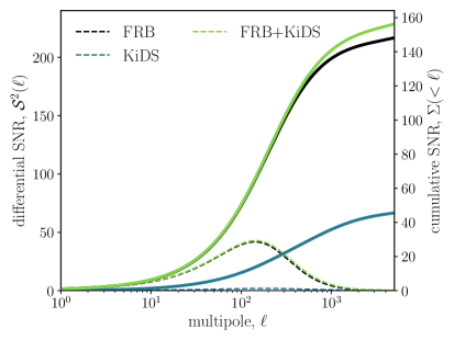
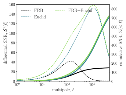
Figure 3: Signal-to-Noise ratio (SNR) for a joint analysis of a cosmic shear survey with DM statistics. dashed lines depict the squared SNR at each multipole, while solid lines show the cumulative SNR below the indicated multipole, $\ell$ (compare to Equation 2.20). Left: for KiDS, Right: for Euclid. Note that the same FRB sample was considered in both cases.

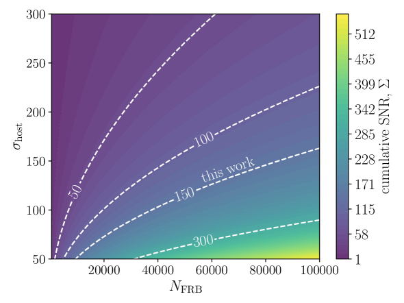
Figure 4: Cumulative SNR as a function of the Noise specification in Equation 2.17, where $\bar{n}=N_{\mathrm{FRB}}/(4\uppi)$. White lines indicate selected curves of constant SNR.

To obtain a better understanding of the significance of each measurement, the SNR curves are shown in Figure 3 as a function of multipole $\ell$. Dashed lines illustrate the squared differential SNR at each multipole, while solid lines show the integrated SNR. In the case of a stage-3 survey such as KiDS, the SNR from the DM correlations is roughly three times as large and picks up signal at larger scales. This is mainly due to the large $f_{\mathrm{sky}}$ in case of the FRBs. Comparing this with Figure 2 we see that, while the noise level is similar for both observables, the smaller area probed by KiDS reduces the overall SNR relative to the FRBs. The green line shows that mainly the small scales add additional signal due to the large correlation between FRBs and lensing. For the state-4 survey the signal is now dominated by cosmic shear. Especially at high multipoles only cosmic shear adds any signal.

Since the DM scatter of the host galaxy, $\sigma_{\mathrm{host}}$, is quite uncertain, the total SNR is shown for different noise levels in Figure 4 where both $\sigma_{\mathrm{host}}$ and $N_{\mathrm{FRB}}$ are varied while the rest of the survey specifications is kept fixed (i.e. the distribution of FRBs along the line-of-sight). It should also be noted that the host contribution follows rather a log-normal than a Gaussian distribution [58, 59] so $\sigma_{\mathrm{host}}$ should be seen as the corresponding variance to that distribution which is an accurate description as long as one is considering 2-point correlations only. The fiducial value of $\sigma_{\mathrm{DM}}=50$ is on the lower end of the plot and it might be considerably larger. On the other hand $N_{\mathrm{FRB}}=10^{4}$ is a conservative estimate for the number of FRBs available at later data releases by Euclid or LSST-Rubin at the end of the decade. We would therefore argue that the SNR assumed here is in reasonable reach in that time span.

Probe	$h$	$\Omega_{\mathrm{cdm}}$	$\sigma_{8}$	$\Omega_{\mathrm{b}}$	$w_{0}$	$w_{1}$	a$\;\mathrm{log}_{10}T_{\mathrm{AGN}}$	$\sum\!m_{\nu}[\mathrm{eV}]$	$n_{\mathrm{s}}$
				Fisher
Euclid	0.1	0.019	0.039	0.015	0.215	0.908	0.208	0.334	0.092
KiDS	0.678	0.026	0.08	0.117	-	-	1.145	-	-
FRB	1.483	1.471	0.958	0.128	9.955	53.246	1.219	2.559	2.018
Euclid+FRB	0.064	0.014	0.022	0.006	0.17	0.677	0.014	0.191	0.037
	($85\;\%)$	($45\;\%)$	($95\;\%)$	($679\;\%)$	($47\;\%)$	($57\;\%)$	($2153\;\%)$	($122\;\%)$	($340\;\%)$
KiDS+FRB	0.041	0.026	0.05	0.006	-	-	1.145	-	-
				MCMC
Prior	$[0.64,0.82]$	$[0.051,0.255]h^{-2}$	$[0.7,1.2]$	$[0.019,0.026]h^{-2}$	$[-1,0]$	$[-1-w_{0},-w_{0}]$	none	$[0,\infty]$	none
Euclid	0.113	0.01	0.016	0.013	0.101	0.237	0.196	0.137	0.117
Euclid + FRB	0.065	0.009	0.012	0.005	0.092	0.21	0.017	0.089	0.051
	$(73\;\%)$	$(5\;\%)$	$(26\;\%)$	$(172\;\%)$	$(10\;\%)$	$(12\;\%)$	$(1020\;\%)$	$(54\;\%)$	$(129\;\%)$

Table 2: One dimensional marginal constraints for 68$\;\%$ confidence on the cosmological and feedback parameters using different survey settings. The first part of the table uses a Fisher analysis with no prior. In the lower part we fit a noiseless data vector with using MCMC and flat priors on the some of the parameters. For the case of Euclid+FRB we also quote the relative reduction of error in percent. Note that the FRB case is only given for the full parameter set.

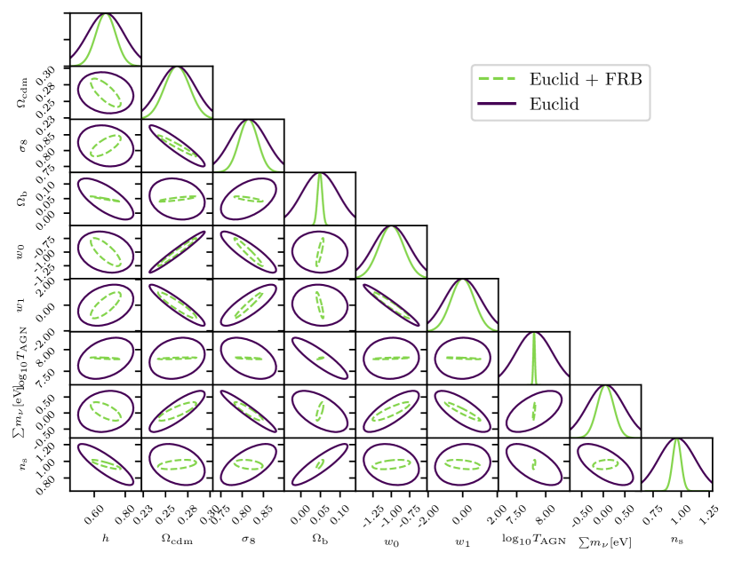
Figure 5: Fisher matrix forecast for Euclid and an FRB survey with $N_{\mathrm{FRB}}=10^{4}$ and $\alpha=3.5$ (compare right panel of Figure 3). Blue contours show the constraints obtainable with, while green contours show the improvement when adding DM correlations. The footprints over which the obsvervables are estimated are assumed to overlap completely. Contours from the FRBs are not shown in this Figure, as they are outperformed for most parameters by cosmic shear in this case.

3.2 Cosmological Constraints

We now analyse a set of 9 (5) cosmological and feedback parameters for a stage-4 and a stage-3 survey respectively, using the setup from the previous section and Table 1. The parameters and the corresponding one dimensional marginal constraints are shown in Table 2. An analogous corner plot is shown in Figure 5 for the case of a stage-4 survey. In general we distinguish two cases: $(i)$ FRB and cosmic shear auto-correlations separately and $(ii)$ FRB plus cosmic shear, also including the cross-correlation measurements. From Figure 3 we already know that a stage-4 cosmic shear survey outperforms the considered FRB sample by almost a factor of 10 in SNR. It is thus expected that constraints on parameters modifying the amplitude of both spectra simultaneously will be dominated by the cosmic shear measurement. This can be seen clearly in Figure 5, where the amplitude of the power spectrum, $\sigma_{8}$, is very well constrained by Euclid. Similarly, one finds that the dark energy equation of state parameters $w_{0}$ and $w_{1}$ assume all the constraining power from the lensing signal as well. This is due to the fact that there is a longer redshift baseline for the cosmic shear survey and more tomographic information. The FRB sample on the other hand requires a lot of its signal to be put into constraining the total amplitude eq. 2.11, leaving almost no constraining power for the other parameters. Note that this drastically changes by using FRBs with host identification [22, 23]. However, we would like to stress that also unlocalised FRBs still add information to the cosmic shear measurements, even to those parameters typically well constrained by lensing alone. As explained below in more detail, this is caused by the tighter constraints on feedback from DM correlations.

Typical parameters weakly constrained by lensing are the Hubble constant, $h$ and the baryon density $\Omega_{\mathrm{b}}$. Since both enter in the amplitude of the DM, it is clear that they can be very well measured with the help of FRBs. The following feature, however, is striking: the constraints on the feedback $\log_{10}T_{\mathrm{AGN}}$ are an order of magnitude better including FRBs compared to cosmic shear alone. The main driver for this effect is that the baryon distribution itself is much more affected by feedback than the total matter distribution which consists mostly of dark matter, making it more inert to feedback. Similar performance can be expected for more complicated feedback models with more model parameters [53, 55]. In fact, for more free parameters of the feedback external constraints will become more and more important. Due to the degeneracy between the sum of neutrino masses, $\sum m_{\nu}$, and the feedback parameter, $\log_{10}T_{\mathrm{AGN}}$, the former will benefit from the increased precision of the latter. Another interesting degeneracy is the primordial slope of the power spectrum, $n_{\mathrm{s}}$. Fixing this slope is important to connect the clustering strength on small scales with the one measured on larger scales. Cosmic shear alone can only achieve this if the feedback is constrained, showing that FRBs help to break this degeneracy is well. Measuring $n_{s}$ precisely is very important for the measurement of scale dependent growth on large scales, as is predicted in many theories of modified gravity.

To mimic a more realistic situation, we create a noiseless data vector for the three spectra and estimate the posterior distribution using Markov Chain Monte Carlo (MCMC) sampled by emcee [60]. We impose some restrictions to the parameter space by imposing priors on the cosmological parameters. This particularly ensures that the nonlinear power spectrum and electron bias are not extrapolated beyond the range of simulations used to calibrate the model (see also table [14]). We also summarise the choices for the flat priors in the lower half of Table 2 together with the marginal $68\%$ confidence intervals obtained by cosmic shear alone and cosmic shear combined with FRBs. The trends are very similar, however, we get in general less improvement. The reason for this is that the prior range injects additional information. It can be seen for example that the posteriors for $h$ or $\Omega_{\mathrm{b}}$ are prior dominated in the cosmic shear case. Also the restriction to non-phantom dark energies and no crossing of $w>0$ reduces the parameter space volume. These effects reduce the gain from adding FRB measurements since degeneracies are already slightly broken by the prior. Nonetheless, we still find an order of magnitude improvement for the constraints on $\log_{10}T_{\mathrm{AGN}}$ and $50\%$ for the neutrino mass. Finally it is worth pointing out that the addition of FRBs also allows cosmic shears to be a more independent probe from the Cosmic Microwave Background (similar to using tSZ) as external priors on the baryon density are not required and the parameter can be fitted simultaneously.

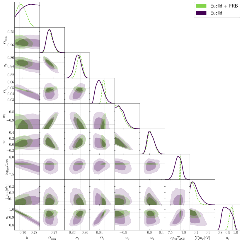
Figure 6: Forecast using a noiseless data vector for Euclid and an FRB survey with $N_{\mathrm{FRB}}=10^{4}$ and $\alpha=3.5$ (compare right panel of Figure 3). Line colours and styles are the same as in Figure 5 with the caveat that the priors from Table 2 are used. The two contours correspond to the standard $68$ and $95\;\%$ confidence intervals.

4 Conclusion

The ability of future weak lensing surveys to address their key scientific questions, including the search for the mass scale of neutrinos, is largely limited by our understanding of the effect of baryonic physics on the clustering of matter on non-linear scales. While these effects can be measured from simulations, they are vastly different depending on the sub-grid model used. In this work, we investigated an alternative probe of the electron power spectrum, which has been accessible only via the tSZ effect so far, the DM angular correlations measured from FRBs. DM correlations are an integrated quantity very similar to cosmic shear, they therefore provides access to very similar scales and can efficiently break degeneracies between cosmological and feedback parameters. Compared to the tSZ effect, DM correlations give different weights to different redshifts and scales. We used a simple feedback prescription with one parameter to model the matter, electron and matter-electron power spectra and investigated the improvements when cross-correlating a stage-4 cosmic shear survey with the DM from $10^{4}$ FRBs, a number easily achievable within the next years. Our main findings can be summarised as follows:

1. The DM of FRB observations can improve the constraints on baryonic feedback by an order of magnitude, depending on the SNR of the detection of the DM correlations. Simultaneously, FRBs also help to constrain the Hubble constant and the baryon density. Combining these effects, the constraints on the neutrino mass can be improved by 50 to 100 percent. The SNR used in this work is well in reach within the next decade considering upcoming observations and dedicated searches for FRBs.

2. DM correlations have a different radial weighting function than tSZ measurements, they are therefore sensitive to different redshifts. Furthermore the observations do not rely directly on the CMB and are hence an entirely different probe at low redshifts with different systematics.

There are a few limiting factors in our analysis. These include a very simple feedback model, Gaussian statistics and the absence of systematic effects. We did not make use of any redshift distribution of FRBs provided by host identification. The scope of this paper, however, is to show that FRBs can be a powerful cosmological probe in particular in conjunction with tracers of the full matter distribution, leveraging the different clustering properties of baryons and dark matter. In the future we intend to tackle the mentioned limitations by considering a more realistic setup for the inference process.

Appendix A Stability of the Fisher matrix

To ensure the stability of the Fisher matrix, we vary the step size with which we evaluate the derivative. This exercise is shown in Figure 7 for two different choices for $\epsilon$. In particular we take the central form of the finite difference and vary the parameters by

$$\delta\theta_{i\pm}=\left\{\begin{array}[]{ll}\theta_{i,0}(1\pm\epsilon)&\;\;\text{if }\;\;\theta_{i,0}\neq 0\\ \pm\epsilon&\;\;\text{else }\end{array}\right.\;,$$ (A.1)

where $\theta_{i,0}$ is the parameter’s fiducial value.

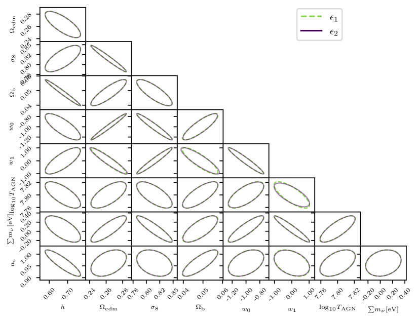
Figure 7: Same as Figure 5 but with varying step size for the numerical derivative. In particular we choose $\epsilon_{3}=10^{-3}$ and $\epsilon_{1}=10^{-2}$ for the green and dark violet lines respectively. The fiducial case in Figure 5 assumes $\epsilon_{1}=5\times 10^{-3}$.

References

- [1] H. Hildebrandt, M. Viola, C. Heymans, S. Joudaki, K. Kuijken, C. Blake et al., KiDS-450: cosmological parameter constraints from tomographic weak gravitational lensing, Monthly Notices of the Royal Astronomical Society 465 (2017) 1454.
- [2] M. Asgari and others, KiDS-1000 Cosmology: Cosmic shear constraints and comparison between two point statistics, Astron. Astrophys. 645 (2021) A104.
- [3] T. M. C. Abbott and others, Dark Energy Survey year 1 results: Cosmological constraints from galaxy clustering and weak lensing, Phys. Rev. D 98 (2018) 043526.
- [4] A. Amon, D. Gruen, M. A. Troxel, N. MacCrann, S. Dodelson, A. Choi et al., Dark Energy Survey Year 3 results: Cosmology from cosmic shear and robustness to data calibration, Phys. Rev. D 105 (2022) 023514 [2105.13543].
- [5] M. Takada, Subaru Hyper Suprime-Cam Project, in American Institute of Physics Conference Series (N. Kawai and S. Nagataki, eds.), vol. 1279 of American Institute of Physics Conference Series, pp. 120–127, Oct., 2010, DOI.
- [6] T. Hamana, M. Shirasaki, S. Miyazaki, C. Hikage, M. Oguri, S. More et al., Cosmological constraints from cosmic shear two-point correlation functions with HSC survey first-year data, Publications of the Astronomical Society of Japan 72 (2020) 16.
- [7] R. S. Somerville and R. Davé, Physical Models of Galaxy Formation in a Cosmological Framework, Annu. Rev. Astron. Astrophys. 53 (2015) 51.
- [8] M. Vogelsberger, F. Marinacci, P. Torrey and E. Puchwein, Cosmological simulations of galaxy formation, Nat Rev Phys 2 (2020) 42.
- [9] N. E. Chisari, M. L. A. Richardson, J. Devriendt, Y. Dubois, A. Schneider, A. M. C. Le Brun et al., The impact of baryons on the matter power spectrum from the Horizon-AGN cosmological hydrodynamical simulation, Monthly Notices of the Royal Astronomical Society 480 (2018) 3962.
- [10] M. P. van Daalen, I. G. McCarthy and J. Schaye, Exploring the effects of galaxy formation on matter clustering through a library of simulation power spectra, Monthly Notices of the Royal Astronomical Society 491 (2020) 2424.
- [11] F. Villaescusa-Navarro, D. Anglés-Alcázar, S. Genel, D. N. Spergel, R. S. Somerville, R. Dave et al., The CAMELS Project: Cosmology and Astrophysics with Machine-learning Simulations, The Astrophysical Journal 915 (2021) 71.
- [12] I. G. McCarthy, J. Schaye, S. Bird and A. M. C. Le Brun, The BAHAMAS project: calibrated hydrodynamical simulations for large-scale structure cosmology, Monthly Notices of the Royal Astronomical Society 465 (2017) 2936.
- [13] A. J. Mead, T. Tröster, C. Heymans, L. Van Waerbeke and I. G. McCarthy, A hydrodynamical halo model for weak-lensing cross correlations, Astron. Astrophys. 641 (2020) A130.
- [14] T. Tröster and others, Joint constraints on cosmology and the impact of baryon feedback: Combining KiDS-1000 lensing with the thermal Sunyaev–Zeldovich effect from Planck and ACT, Astron. Astrophys. 660 (2022) A27.
- [15] A. Nicola, F. Villaescusa-Navarro, D. N. Spergel, J. Dunkley, D. Anglés-Alcázar, R. Davé et al., Breaking baryon-cosmology degeneracy with the electron density power spectrum, J. Cosmol. Astropart. Phys. 2022 (2022) 046.
- [16] D. Thornton, B. Stappers, M. Bailes, B. Barsdell, S. Bates, N. D. R. Bhat et al., A Population of Fast Radio Bursts at Cosmological Distances, Science 341 (2013) 53.
- [17] E. Petroff, M. Bailes, E. D. Barr, B. R. Barsdell, N. D. R. Bhat, F. Bian et al., A real-time fast radio burst: polarization detection and multiwavelength follow-up, MNRAS 447 (2015) 246.
- [18] L. Connor, J. Sievers and U.-L. Pen, Non-cosmological FRBs from young supernova remnant pulsars, Monthly Notices of the Royal Astronomical Society 458 (2016) L19.
- [19] D. J. Champion, E. Petroff, M. Kramer, M. J. Keith, M. Bailes, E. D. Barr et al., Five new fast radio bursts from the HTRU high-latitude survey at Parkes: first evidence for two-component bursts, Monthly Notices of the Royal Astronomical Society 460 (2016) L30.
- [20] S. Chatterjee, C. J. Law, R. S. Wharton, S. Burke-Spolaor, J. W. T. Hessels, G. C. Bower et al., A direct localization of a fast radio burst and its host, Nature 541 (2017) 58.
- [21] B. Zhou, X. Li, T. Wang, Y.-Z. Fan and D.-M. Wei, Fast radio bursts as a cosmic probe?, Phys. Rev. D 89 (2014) 107303.
- [22] A. Walters, A. Weltman, B. M. Gaensler, Y.-Z. Ma and A. Witzemann, Future Cosmological Constraints From Fast Radio Bursts, The Astrophysical Journal 856 (2018) 65.
- [23] S. Hagstotz, R. Reischke and R. Lilow, A new measurement of the Hubble constant using fast radio bursts, Mon. Not. Roy. Astron. Soc. 511 (2022) 662.
- [24] J.-P. Macquart, J. X. Prochaska, M. McQuinn, K. W. Bannister, S. Bhandari, C. K. Day et al., A census of baryons in the Universe from localized fast radio bursts, Nature 581 (2020) 391.
- [25] Q. Wu, G.-Q. Zhang and F.-Y. Wang, An 8 per cent determination of the Hubble constant from localized fast radio bursts, Monthly Notices of the Royal Astronomical Society 515 (2022) L1.
- [26] C. W. James, E. M. Ghosh, J. X. Prochaska, K. W. Bannister, S. Bhandari, C. K. Day et al., A measurement of Hubble’s Constant using Fast Radio Bursts, Monthly Notices of the Royal Astronomical Society 516 (2022) 4862.
- [27] R. Reischke and S. Hagstotz, Consistent constraints on the equivalence principle from localized fast radio bursts, MNRAS 523 (2023) 6264 [2302.10072].
- [28] R. Reischke and S. Hagstotz, Covariance Matrix of Fast Radio Bursts Dispersion, Jan., 2023. 10.48550/arXiv.2301.03527.
- [29] K. W. Masui and K. Sigurdson, Dispersion Distance and the Matter Distribution of the Universe in Dispersion Space, Physical Review Letters 115 (2015) 121301.
- [30] M. Shirasaki, K. Kashiyama and N. Yoshida, Large-scale clustering as a probe of the origin and the host environment of fast radio bursts, Physical Review D 95 (2017) 083012.
- [31] M. Rafiei-Ravandi, K. M. Smith, D. Li, K. W. Masui, A. Josephy, M. Dobbs et al., CHIME/FRB Catalog 1 results: statistical cross-correlations with large-scale structure, arXiv:2106.04354 [astro-ph] (2021) .
- [32] M. Bhattacharya, P. Kumar and E. V. Linder, Fast Radio Burst Dispersion Measure Distribution as a Probe of Helium Reionization, arXiv:2010.14530 [astro-ph] (2020) .
- [33] R. Takahashi, K. Ioka, A. Mori and K. Funahashi, Statistical modelling of the cosmological dispersion measure, Mon. Not. Roy. Astron. Soc. 502 (2021) 2615.
- [34] R. Reischke, S. Hagstotz and R. Lilow, Probing primordial non-Gaussianity with Fast Radio Bursts, Phys. Rev. D 103 (2021) 023517.
- [35] R. Reischke, S. Hagstotz and R. Lilow, Consistent equivalence principle tests with fast radio bursts, Monthly Notices of the Royal Astronomical Society 512 (2022) 285.
- [36] S. Johnston, R. Taylor, M. Bailes, N. Bartel, C. Baugh, M. Bietenholz et al., Science with ASKAP - the Australian Square Kilometre Array Pathfinder, Exp Astron 22 (2008) 151.
- [37] R. Maartens, F. B. Abdalla, M. Jarvis, M. G. Santos and f. t. SKA Cosmology SWG, Cosmology with the SKA – overview, ArXiv e-prints (2015) .
- [38] M. Caleb, C. Flynn, M. Bailes, E. D. Barr, T. Bateman, S. Bhandari et al., Fast Radio Transient searches with UTMOST at 843 MHz, Monthly Notices of the Royal Astronomical Society 458 (2016) 718.
- [39] L. B. Newburgh, K. Bandura, M. A. Bucher, T.-C. Chang, H. C. Chiang, J. F. Cliche et al., HIRAX: A Probe of Dark Energy and Radio Transients, arXiv:1607.02059 [astro-ph] (2016) 99065X.
- [40] J. M. Yao, R. N. Manchester and N. Wang, A New Electron-density Model for Estimation of Pulsar and FRB Distances, The Astrophysical Journal 835 (2017) 29.
- [41] D. N. Limber, The Analysis of Counts of the Extragalactic Nebulae in Terms of a Fluctuating Density Field. II., ApJ 119 (1954) 655.
- [42] M. Loverde and N. Afshordi, Extended Limber approximation, Phys. Rev. D 78 (2008) 123506.
- [43] C. D. Leonard and others, The N5K Challenge: Non-Limber Integration for LSST Cosmology, .
- [44] A. J. Mead, J. A. Peacock, C. Heymans, S. Joudaki and A. F. Heavens, An accurate halo model for fitting non-linear cosmological power spectra and baryonic feedback models, MNRAS 454 (2015) 1958.
- [45] A. Blanchard and others, Euclid preparation: VII. Forecast validation for Euclid cosmological probes, Astron. Astrophys. 642 (2020) A191.
- [46] B. Joachimi, C. A. Lin, M. Asgari, T. Tröster, C. Heymans, H. Hildebrandt et al., KiDS-1000 methodology: Modelling and inference for joint weak gravitational lensing and spectroscopic galaxy clustering analysis, AAP 646 (2021) A129 [2007.01844].
- [47] E. Platts, J. X. Prochaska and C. J. Law, A Data-driven Technique Using Millisecond Transients to Measure the Milky Way Halo, The Astrophysical Journal 895 (2020) L49.
- [48] A. A. Meiksin, The physics of the intergalactic medium, Reviews of Modern Physics 81 (2009) 1405.
- [49] G. D. Becker, J. S. Bolton, M. G. Haehnelt and W. L. W. Sargent, Detection of extended He II reionization in the temperature evolution of the intergalactic medium, Monthly Notices of the Royal Astronomical Society 410 (2011) 1096.
- [50] J. M. Shull, B. D. Smith and C. W. Danforth, The Baryon Census in a Multiphase Intergalactic Medium: 30% of the Baryons May Still be Missing, The Astrophysical Journal 759 (2012) 23.
- [51] C. W. James, J. X. Prochaska, J.-P. Macquart, F. North-Hickey, K. W. Bannister and A. Dunning, The z–DM distribution of fast radio bursts, Monthly Notices of the Royal Astronomical Society 509 (2021) 4775.
- [52] A. M. C. Le Brun, I. G. McCarthy, J. Schaye and T. J. Ponman, Towards a realistic population of simulated galaxy groups and clusters, Monthly Notices of the Royal Astronomical Society 441 (2014) 1270.
- [53] R. E. Angulo, M. Zennaro, S. Contreras, G. Aricò, M. Pellejero-Ibañez and J. Stücker, The BACCO simulation project: exploiting the full power of large-scale structure for cosmology, Monthly Notices of the Royal Astronomical Society 507 (2021) 5869.
- [54] G. Aricò, R. E. Angulo, C. Hernández-Monteagudo, S. Contreras and M. Zennaro, Simultaneous modelling of matter power spectrum and bispectrum in the presence of baryons, Monthly Notices of the Royal Astronomical Society 503 (2021) 3596.
- [55] G. Aricò, R. E. Angulo, S. Contreras, L. Ondaro-Mallea, M. Pellejero-Ibañez and M. Zennaro, The BACCO simulation project: a baryonification emulator with neural networks, Monthly Notices of the Royal Astronomical Society 506 (2021) 4070.
- [56] M. Tegmark, A. N. Taylor and A. F. Heavens, Karhunen-Loève Eigenvalue Problems in Cosmology: How Should We Tackle Large Data Sets?, ApJ 480 (1997) 22.
- [57] H. Hildebrandt, J. L. van den Busch, A. H. Wright, C. Blake, B. Joachimi, K. Kuijken et al., KiDS-1000 catalogue: Redshift distributions and their calibration, AAP 647 (2021) A124 [2007.15635].
- [58] Z. J. Zhang, K. Yan, C. M. Li, G. Q. Zhang and F. Y. Wang, Intergalactic medium dispersion measures of fast radio bursts estimated from IllustrisTNG simulation and their cosmological applications, Astrophys. J. 906 (2021) 49.
- [59] J.-F. Mo, W. Zhu, Y. Wang, L. Tang and L.-L. Feng, The dispersion measure of Fast Radio Bursts host galaxies: estimation from cosmological simulations, Mon. Not. Roy. Astron. Soc. 518 (2022) 539.
- [60] D. Foreman-Mackey, D. W. Hogg, D. Lang and J. Goodman, emcee: The MCMC Hammer, Publications of the Astronomical Society of the Pacific 125 (2013) 306.