Latent assimilation with implicit neural representations
for unknown dynamics

Abstract

Data assimilation is crucial in a wide range of applications, but it often faces challenges such as high computational costs due to data dimensionality and incomplete understanding of underlying mechanisms. To address these challenges, this study presents a novel assimilation framework, termed Latent Assimilation with Implicit Neural Representations (LAINR). By introducing Spherical Implicit Neural Representations (SINR) along with a data-driven uncertainty estimator of the trained neural networks, LAINR enhances efficiency in assimilation process. Experimental results indicate that LAINR holds certain advantage over existing methods based on AutoEncoders, both in terms of accuracy and efficiency.

Keywords— data assimilation, implicit neural representation, spherical harmonics, uncertainty estimation

1 Introduction

Data assimilation (DA) has increasingly become an essential tool across a multitude of disciplines, including but not limited to weather forecasting, climate modeling, oceanography, ecology, and even economics [38, 40, 54, 50, 53]. It aims to integrate information from various data sources, such as in-situ measurements, satellite and radar observations [41], with existing physical models that describe a system’s underlying dynamics. The objective of DA is to obtain the best estimate of the system states, while accounting for uncertainties in both observations and physical models.

From a mathematical standpoint, DA offers an efficient and practical solution to a specific type of optimal control problem [5]

$$\begin{cases}\dot{\bm{x}}(t)=\mathcal{M}(\bm{x}(t),t)+\bm{\varepsilon}^{M}(t),&0\leq t\leq T,\\ \bm{x}(0)=\bm{u}\end{cases}$$ (1)

with the objective function

$$\bm{J}(\bm{u})=\mathcal{L}_{B}(\bm{u},\bm{x}^{b})+\int_{0}^{T}\mathcal{L}_{O}(\mathcal{H}(\bm{x}(t)),\bm{y}(t))\mathrm{d}t+\int_{0}^{T}\mathcal{L}_{E}\left(\bm{\varepsilon}^{M}(t)\right)\mathrm{d}t.$$ (2)

Here, the system dynamics is denoted by $\mathcal{M}$, and $\mathcal{H}$ stands for the observation operator. $\mathcal{L}_{B}$ and $\mathcal{L}_{O}$ penalize the discrepancy between the system states and the background estimate $\bm{x}^{b}$ and the observation data $\bm{y}(t)$, while $\mathcal{L}_{E}$ penalize the model error $\bm{\varepsilon}^{M}(t)$. The goal is to find the optimal control $\bm{u}$ as the initial system state that minimizes the objective function $\bm{J}(\bm{u})$. For instance, in the realm of modern numerical weather prediction (NWP), $\bm{x}(t)$ may consist of the meteorological variables over multiple time steps governed by atmospherical dynamics, then DA frameworks are employed to determine the optimal system states for further prediction.

Early efforts for DA primarily revolved around techniques like the nudging and optimal (statistical) interpolation methods. Subsequently, variational methods (3/4D-Var) have been proposed based on the optimal control theory. A key advantage of the variational approaches lies in their ability to make meteorological fields comply with the dynamical equations of NWP models, while simultaneously minimizing the discrepancies between simulations and observations. However, these methods are often computationally intensive, particularly for high-dimensional systems. Additionally, the necessity to derive the corresponding tangent linear models and adjoint models becomes another challenge especially for complex dynamics.

Another advanced development of DA frameworks is the proposal of Kalman Filter (KF) methods [27, 5], which facilitate sequential assimilation of data, and thus offer benefit for real-time applications. Literatures such as [72] have shown that Kalman filtering is equivalent to variational assimilation in some limit. Unfortunately, the challenge of high-dimensionality persists in that the scales of computational grid and the underlying matrices are linked to the state dimension. Some approximate or suboptimal Kalman filters have been developed to partially alleviate the issue, but at the expense of confining the assimilated states within a low-dimensional subspace, potentially harming the overall performance.

Moreover, existing DA frameworks rely on accurate dynamical cores, but capturing small-scale physical processes or edge effects, especially where the physical knowledge is limited and no well-designed parameterizations are available is still a challenge, which will probably lead to significant and undetermined model error. Another significant obstacle arises when dealing with highly non-linear systems. The inherent difficulties in optimizing non-convex problems and the inconsistency with the linear assumptions of the Kalman filter point to a need for more advanced DA techniques.

One approach to handle the high-dimensionality issue is by means of Reduced-Order-Models (ROMs), which establish a lower-dimensional parameterization space and then shift the DA framework to the latent space. Classical ROMs usually employ linear trial subspaces for model reduction, but they require lower-dimensioanl subspaces of dimension much larger than the intrinsic dimension of the solution manifold to ensure high accuracy especially for highly non-linear problems [55]. Based on the Kolmogorov $n$-width [63], [24] has proposed a continuous non-linear version

$$d_{n}(\mathcal{S})=\inf_{\begin{subarray}{c}P:\mathcal{S}\to\mathbb{R}^{n}\\ Q:\mathbb{R}^{n}\to\mathcal{S}\end{subarray}}\sup_{f\in\mathcal{S}}\|f-Q(P(f))\|$$ (3)

to quantify the intrinsic complexity of a compact functional space $K$, which together with the recent work [44, 30, 79] shows the theoretical superiority of non-linear ROMs over linear ones.

Machine learning (ML), and specifically Deep Learning (DL) emerges as an effective data-driven tool to approximate high-dimensional mappings thanks to its strengths to extract intricate structures in high-dimensional data [43], and consequently, neural networks are used not only to establish non-linear ROMs, whose training processes depend on reconstruction loss functions similar to (3) where the mappings $P$ and $Q$ are translated as parameterized encoder and decoder, but also to learn the corresponding reduced or latent dynamics [33, 67, 17] from encoded data.

With an appropriate temporal discretization on the latent dynamics, the original DA problem turns

$$\begin{cases}\bm{z}_{k+1}=\mathcal{G}_{\bm{\psi}}(\bm{z}_{k})+\bm{\varepsilon}^{L}_{k},&k=0,1,\cdots,\\ \bm{z}(0)=\bm{u}\end{cases}$$ (4)

subject to

$$\bm{z}_{k}=\mathcal{E}_{\bm{\theta}}(\bm{x}_{k}),\,\bm{x}_{k}=\mathcal{D}_{\bm{\varphi}}(\bm{z}_{k})+\bm{\varepsilon}_{k}^{\textrm{E-D}}$$ (5)

with the objective function

$$\bm{J}(\bm{u},\bm{\theta},\bm{\varphi},\bm{\psi})=\mathcal{L}_{B}(\bm{u},\bm{z}^{b})+\sum_{k}\mathcal{L}_{O}(\mathcal{H}\left(\mathcal{D}_{\bm{\varphi}}(\bm{x}_{k})\right),\bm{y}_{k})+\sum_{k}\mathcal{L}_{E}^{L}\left(\bm{\varepsilon}_{k}^{L}\right)+\sum_{k}\mathcal{L}_{\textrm{E-D}}(\bm{\varepsilon}_{k}^{\textrm{E-D}}).$$ (6)

The latent dynamics $\mathcal{G}_{\bm{\psi}}$ is parameterized by $\bm{\psi}$, and $\mathcal{E}_{\bm{\theta}}:\mathcal{X}^{\prime}\to\mathcal{Z}$ and $\mathcal{D}_{\bm{\varphi}}:\mathcal{Z}\to\mathcal{X}^{\prime}$ are the encoder and decoder networks parameterized by $\bm{\theta}$ and $\bm{\varphi}$ respectively. $\mathcal{L}_{E}^{L}$ penalize the error $\bm{\varepsilon}_{k}^{L}$ for the latent model, and $\mathcal{L}_{\textrm{E-D}}$ penalize the reconstruction error $\bm{\varepsilon}_{k}^{\textrm{E-D}}$ for the encoder-decoder mappings. Such a transition for DA from physical space to latent space is referred to as the latent assimilation (LA) [1]. No expert knowledge is needed for constructing the dynamical model, and it has the benefit of reducing both the storage and computational demands of LA compared with traditional methods.

In recent years, the rapid development of DL has had a transformative impact on various domains, including computer vision, natural language processing, and more recently scientific computing. The applications of DL in solving complex physical problems, such as solving differential equations [64, 76, 70], discovering underlying physical laws [47, 12, 75], and simulating spatio-temporal dynamics [48, 45], have attracted significant attention and achieved promising results. In the specific area of atmospheric sciences, DL has proven itself highly effective in handling a variety of tasks, ranging from weather nowcasting and forecasting to post-processing and data assimilation. Specifically, the success of forecast models like FourCastNet [58], Pangu-Weather [11], GraphCast [42] and FengWu [15] focusing on learning a surrogate dynamics has gradually dissolved the initial doubts [69] regarding DL’s capability to handle complex dynamics.

In this work, we present the Latent Assimilation with Implicit Neural Representations (LAINR) framework (Figure 1). Our framework is designed to assimilate data from systems with partially or even completely unknown dynamics. By proposing a new variant of the implicit neural representation, namely the Spherical Implicit Neural Representation (SINR), and a comprehensive assimilation procedure for learning surrogate models and estimating corresponding uncertainties, we aim to make a meaningful contribution to the ongoing exploration of DL and ML techniques in data assimilation and atmospheric sciences.

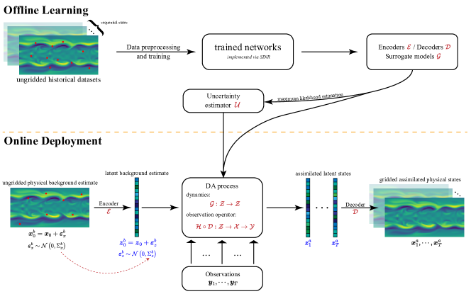
Figure 1: The pipeline of the LAINR framework.

1.1 Related works and contributions

Reduced-order models

The concept of Reduced-Order Models (ROMs) is not a new idea for data assimilation. As introduced previously, dimensionality reduction techniques are employed to represent high-dimensional vectors with lower-dimensional ones. Classical ROMs usually rely on linear methods like Proper Orthogonal Decomposition (POD) [14, 4, 3] or wavelet decomposition [74] to extract system’s dominant modes from historical snapshots, then the corresponding parameterizations $\bm{z}\in\mathcal{Z}$ for each state $\bm{x}\in\mathcal{X}^{\prime}\subseteq\mathcal{X}$ are the projection coefficient vectors onto each mode. Recently, DL advancements have offered alternative approaches to construct or enhance ROMs. AutoEncoders [8, 81] are one of the most common methods to learn a non-linear, low-dimensional representation of the high-dimensional data, and the learned representations can then be used to study and understand the behavior of the system at a lower computational cost [44, 30]. Meanwhile, Recurrent Neural Networks (RNNs) [46] including the Long Short-Term Memory (LSTM) networks [36] and the Gated Recurrent Unit (GRU) networks [22] have also been employed to model time-dependent problems and capture the temporal correlations in the training data.

Latent assimilation

Latent assimilation has also benefited from the advent of DL, particularly in constructing non-linear encoder-decoder mappings for assimilation in latent space. For instance, previous reseach [62] selects simple fully-connected deep neural networks for both the encoder and the decoder, with ReZero [7] as a variant of ResNet [34] to enhance the stability of learning the laten dynamics. In spite of its effectiveness of dimensionality reduction, it is faced with scalability limitations since the fully-connected architecture can hardly be applied to multi-dimensional cases due to the unaffordable costs of the storage and training for the huge number of network parameters. Recurrent Neural Networks (RNNs) can serve as an alternative way for merging the encoder-decoder structure and evolving latent dynamics simultaneously as proposed in [60]. The training of RNNs takes the advantage of Reservoir Computing (RC) [49] to make the forward propagation faster, but as suggested in [2, 60], the RC approaches are more suitable for short-term prediction tasks. Meanwhile, creating patches when scaling up to high-dimensional problems will probably result in disagreement between neighborhoods. To effectively capture long-term dependencies in sequential data, LSTM architectures have been employed in [59, 21], but they face the same issues as those of [62] that the model is not scalable to high-dimensional problems. Finally, all the the architectures mentioned above require the input data lying on certain fixed grids, and the inevitable interpolation procedures probably bring additional errors. Table 1 summarizes the comparative strengths and weaknesses of these methods as well as our proposed framework introduced later.

Table 1: Comparison of different methods for latent assimilation. The method names are borrowed from the original papers.

method	encoder-decoder	latent dynamics	scalability	efficiency	flexibility
ETKF-Q-L [62]	fully-connected	ReZero	low	high	no
RNN-ETKF [60]	RNN	RC	medium	high	no
NIROM-DA [59]	POD/PCA	LSTM	low	medium	no
GLA [21]	POD/PCA + Conv1d	LSTM	low	medium	no
LAINR (ours)	SINR	Neural ODE	high	medium	yes

Implicit neural representations

Implicit Neural Representations (INRs) have emerged as a effective tool for encoding high-dimensional data, geometrical objects, or even functions in a compact and parameterized manner. Diverging from common neural networks representing data in the form of grids or graphs, INRs model them as a continuous functional form. This approach has shown its superiority in a variety of applications, including shape modeling [20, 56], image processing [71, 9, 26], and spatio-temporal dynamics [37, 16, 80]. One key advantage of INRs lie in their agnosticism to any predetermined grid or spatial resolution, thereby gives a high degree of flexibility. Moreover, similar to AutoEncoders, the non-linearity inherent to neural networks enables them to capture the non-linear correlations, which has more potentials than classical linear ROMs such as POD. In this work, we propose a new variant of INRs, namely the Spherical Implicit Neural Representations (SINRs), which aims to capture the complex dynamics of the system in a low-dimensional latent space based on the spherical harmonics defined on the 2D sphere.

The key aspects of our contributions can be summarized as below.

• A Novel Mesh-free DA framework: We present a new assimilation framework named Latent Assimilation with Implicit Neural Representation (LAINR), which is mesh-free and applicable to multi-dimensional unknown dynamics.

  • SINRs. We have formulated a specialized variant of INRs called the Spherical Implicit Neural Representations (SINRs) to handle 2D spherical data. SINRs effectively capture the system’s complex dynamics in a low-dimensional latent space, while ensuring high accuracy and reliable convergence guarantee.

  • Uncertainty Estimation. A novel uncertainty qualification method has been developed to estimate uncertainties associated with both the latent surrogate model and the encoding process, leveraging maximum likelihood estimation (MLE) techniques.

• Interoperability with Existing DA Algorithms: LAINR has been engineered for compatibility to work seamlessly with existing data assimilation algorithms, thereby enhancing the performances and extending their applications. This encourages wider adoption for future advancements in this field.

• Experimental Validation: We have conducted experiments on multi-dimensional cases, including an ideal shallow-water model and a real meteorological dataset to demonstrate the superiority of LAINR compared to existing AutoEncoder-based methods. The effectiveness of LAINR in capturing spatio-temporal dynamics and seamlessly integrating with existing DA algorithms is emphasized in these empirical findings.

The remainder of this paper is structured as follows. Section 2 provides an overview of the existing LA frameworks and then discusses their limitations. Section 3 presents the proposed LAINR framework in detail, which is followed by Section 4 that describes the experimental setup and discusses the results. Finally, Section 5 concludes the superiority of our LAINR framework and outlines some of the potential avenues for future research.

2 Latent assimilation

Latent Assimilation (LA) is essentially a specialized form of Data Assimilation (DA) methodology which makes use of dimensionality reduction of the assimilation space and consequently decreases computational and storage costs. It characterizes the high-dimensional model space, denoted by $\mathcal{X}$, with a more compact, lower-dimensional latent space, denoted by $\mathcal{Z}$. Like conventional DA methodologies, LA also requires a well-defined forward propagation mechanism within the latent space $\mathcal{Z}$ and an associated observation operator that links $\mathcal{Z}$ to the observational space $\mathcal{Y}$ (Figure 2). Additionally, the uncertainties brought by noise must be accounted for within these mappings.

(a) classical DA that operates on the physical space

(b) LA that operates on the latent space

Figure 2: Comparison between classical DA and LA frameworks. Red arrows and blue arrows represent the forward integrators and the observation operators, respectively. The temporal indices are omitted for simplicity.

With the assumption that a low-dimensional parameterization exists for the high-dimensional system states, LA framework explores suitable latent embeddings and surrogate models for the latent dynamics. Let $\mathcal{X}=\mathbb{R}^{n}$ and $\mathcal{Z}=\mathbb{R}^{m}$ be the system state space and the latent space, respectively, where $n$ is considerably larger than $m$. The goal is to identify an encoder $\mathcal{E}:\mathcal{X}^{\prime}\to\mathcal{Z}$ and a decoder $\mathcal{D}:\mathcal{Z}\to\mathcal{X}^{\prime}$ that function as appropriate inverse mappings between the low-dimensional submanifold $\mathcal{X}^{\prime}$ encapsulating all possible system states, and the latent space $\mathcal{Z}$. Assume that the target system state variable of assimilation is $\bm{u}:\mathbb{R}^{d}\to\mathbb{R}^{c}$, where $d$ signifies the intrinsic dimension of the system (usually $2$ or $3$), and $c$ refers to the number of features under consideration, such as horizontal wind, temperature, humidity, and so forth. For a fixed sampling set $S\subseteq\mathbb{R}^{d}$, several strategies can be established to construct ROMs for the system state $\bm{x}=\{\bm{u}(\bm{p})\}_{\bm{p}\in S}\in\mathbb{R}^{|S|\times c}=\mathbb{R}^{n}$.

2.1 Embeddings from physical spaces to latent spaces

2.1.1 Classical linear ROMs

Linear Reduced-Order Models (ROMs) for representing system states have been extensively studied in the literature. By fixing a collection of basis functions or vectors $\{\bm{\phi}_{j}\}_{j}$, the system state $\bm{x}$ is approximated as a linear combination of the basis vectors

$$\bm{x}\approx\sum_{j=1}^{m}c_{j}\bm{\phi}_{j},$$ (7)

where $c_{j}$ denotes the coefficient of the $j$-th basis vector and $m$ is the reduced dimension. In this context, the state $\bm{x}$ is encoded as a lower-dimensional vector $\bm{c}=(c_{1},\cdots,c_{m})^{\mathsf{T}}$. Principal Orthogonal Decomposition (POD) is one such method that determines these basis vectors by minimizing the associated projection errors. Alternatively, multi-scale analysis makes use of fourier modes, spectral modes or wavelets to achieve similar linear approximations under certain truncation operations. Here, we take the method of POD as an example. POD aims to determine a set of orthogonal basis vectors $\{\bm{\phi}_{j}\}_{j=1}^{m}\subseteq\mathbb{R}^{n}$, referred to as dominant modes, that minimize the expectation of the projection error. Formally, given a historical set of ground truths or assimilated data $\{\bm{x}_{k}\}_{k=1}^{K}$, POD solves the optimization problem

$$\{\bm{\phi}_{j}\}_{j=1}^{m}=\operatorname*{argmin}_{\bm{\phi}_{j}}\operatorname*{\mathbb{E}}_{\bm{x}\sim\mathcal{D}_{\mathrm{dist}}}\|\bm{x}-\widehat{\bm{x}}\|^{2}$$ (8)

to determine the dominant modes, where $\mathcal{D}_{\mathrm{dist}}$ denotes the distribution of system states $\bm{x}\in\mathcal{X}$, and $\widehat{\bm{x}}$ is the projection of $\bm{x}$ onto the linear subspace spanned by $\{\bm{\phi}_{j}\}_{j=1}^{m}$. $m$ is the number of dominant modes usually fixed in advance. By solving the optimization problem in an empirical manner, we can reformulate it as

$$\bm{A}:=(\bm{\phi}_{1},\cdots,\bm{\phi}_{m})^{\mathsf{T}}=\operatorname*{argmin}_{\bm{A}}\frac{1}{K}\sum_{k=1}^{K}\left\|\bm{x}_{k}-\bm{A}^{\mathsf{T}}\bm{A}\bm{x}_{k}\right\|^{2}=\operatorname*{argmin}_{A}\sum_{k=1}^{K}\left\|\left(\bm{I}_{n}-\bm{A}^{\mathsf{T}}\bm{A}\right)\bm{x}_{k}\right\|^{2}\textrm{ s.t. }\bm{A}\bm{A}^{\mathsf{T}}=\bm{I}_{m},$$ (9)

which can be solved by applying Singular Value Decomposition (SVD) to $\bm{X}\bm{X}^{\mathsf{T}}$. More specifically, the target function is minimized when the rows of $\bm{A}$ coincide with the first $m$ left singular vectors of the matrix $\bm{X}=(\bm{x}_{1},\cdots,\bm{x}_{K})\in\mathbb{R}^{n\times K}$ (See Proposition A.1 for a detailed proof).

In the context of linear ROMs, each state $\bm{x}$ is parameterized in the latent space $\mathcal{Z}$ bas the projection coefficients corresponding with the dominant modes. For POD, the corresponding encoder and decoder are formulated as

$$\mathcal{E}^{\textrm{POD}}(\bm{x})=\bm{A}\bm{x},\quad\mathcal{D}^{\textrm{POD}}(\bm{z})=\bm{A}^{\mathsf{T}}\bm{z}.$$ (10)

Linear ROMs are not only straightforward to implement, but also offer simple linear bijective mappings between $\mathcal{Z}$ and $\mathcal{X}^{\prime}$, which simplify the derivation of the latent dynamics on $\mathcal{Z}$ as long as the physical dynamics is provided. However, the reconstruction accuracy is heavily dependent on the number of dominant modes, and as the system grow in complexity and non-linearity, much more dominate modes are required to capture the small-scale structures, which diminishing the intended benefit of dimensionality reduction.

2.1.2 AutoEncoders

AutoEncoder (AE), as a common architecture in deep learning, serves as a viable non-linear method for dimensionality reduction. With the encoder and the decoder

$$\mathcal{E}^{\textrm{AE}}(\bm{x})=f_{\bm{\theta}}(\bm{x}),\quad\mathcal{D}^{\textrm{AE}}(\bm{z})=g_{\bm{\varphi}}(\bm{z})$$ (11)

implemented via neural networks, such architecture can skillfully extract more tractable lower-dimensional latent representations from high-dimensional input data. The encoder progressively decreases the data dimension with its multi-layered structure. By mirroring the encoder’s architecture, the decoder takes the encoded representations and then reconstruct the original input data.

The AutoEncoder’s objective is to minimize the empirical reconstruction error by employing a loss function to measure the divergence between the input and reconstructed data. The optimization process for

$$\bm{\theta},\bm{\varphi}=\operatorname*{argmin}_{\bm{\theta},\bm{\varphi}}\sum_{k=1}^{N}\mathcal{L}(\bm{x}_{k},g_{\bm{\varphi}}(f_{\bm{\theta}}(\bm{x}_{k})))$$ (12)

promotes the learning of compressed meaningful data representation. Once both the encoder $f_{\bm{\theta}}$ and the decoder $g_{\bm{\varphi}}$ are trained, $\bm{z}_{k}=f_{\bm{\theta}}(\bm{x}_{k})$ is the corresponding latent representation of $\bm{x}_{k}$, and the decoder $g_{\bm{\varphi}}$ can be used to reconstruct the original data $\bm{x}_{k}$ from $\bm{z}_{k}$ conversely.

Compared with classical linear ROMs, AutoEncoders are capable of capturing non-linear relationships in the data, thereby allowing for the possibility of reducing complex dynamicals system in physical space to a simpler latent dynamics. Despite the promise of AutoEncoders, serveral limitations still persist. Unlike classical linear ROMs, AutoEncoders do not offer an optimal representation since the minimizer is not guaranteed to be obtained. They may also encounter scalability challenges when dealing with high-dimensional problems as the number of grid points will increase exponentially with respect to the state dimension and resolutions. Such complexity could lead to resource-intensive training processes. Moreover, AutoEncoders are generally designed to operate on inputs with fixed structural attributes, limiting their utility in real-world applications that frequently involve partially missing data, ungridded data, or data with varying resolutions.

2.2 Evolution of latent dynamics

Establishing a suitable surrogate model for the evolution of latent dynamics forms another crucial part for the LA framework, which not only accounts for the system’s inherent non-linearity but also incorporates the auto-regressive nature of the latent dynamics evolution, regardless of whether or not the explicit form of the physical dynamics are provided. We simplify our discussion by assuming time-invariant latent dynamics, which is then approximated by a parameterized surrogate model $\mathcal{G}_{\bm{\psi}}$. The goal is to minimize the differences between subsequent latent states, $\bm{z}_{k+1}$ and $\mathcal{G}_{\bm{\psi}}(\bm{z}_{k})$. While linear regression serves as a straightforward method for constructing the latent surrogate model, its performance is limited in describing highly non-linear dynamics. As an alternative, neural networks offer a common data-driven approach to capturing the non-linear relationships in the data and approximating the latent dynamics.

The choices for the structure of $\mathcal{G}_{\bm{\psi}}$ can be quite diverse, depending on the specific characteristics of the system state’s temporal dynamics. For instance, Long Short-Term Memory (LSTM) [36] and Gated Recurrent Units (GRUs) [22] networks are specially designed for sequential data, whose structures enable the network to remember or forget past states based on the context, and the work of [59, 21] has followed such way. Another kinds of modeling the sequential data are motivated by the classical numerical integrators for differential equations. Embedding the physical states into a latent space naturally leads to an unknown latent dynamics, which can be written as

$$\frac{\mathrm{d}\bm{z}}{\mathrm{d}t}=\bm{F}(\bm{z}),$$ (13)

but the latent dynamics cannot be transfered and then established directly from the physical space if the physical dynamics is unknown. By using certain forward integrators such as the Euler method, the latent dynamics can be discretized as

$$\bm{z}_{k+1}\approx\bm{z}_{k}+\bm{F}(\bm{z}_{k})\Delta t\approx\bm{z}_{k}+f_{\bm{\psi}}(\bm{z}_{k})\Delta t=:\mathcal{G}_{\bm{\psi}}(\bm{z}_{k}).$$ (14)

The function $f_{\bm{\psi}}$ used to approximate $\bm{F}$ is implemented with a neural network and the trainable parameters are denoted by $\bm{\psi}$. The update formula coincides with that of ResNet [34], initially promoted to accelerate the training process of deep networks through skip connections that alleviate the problems of vanishing and exploding gradients. ResNet-based architectures have been adapted to learn the latent dynamics [62] via ReZero [7] to enhance the performance. However, such discretization methods are subject to temporal resolution and step size constraints, and applying them directly to real-world assimilation deployment with varing time steps may introduce additional errors.

2.3 Assimilation in latent spaces

The LA frameworks parallel classical DA frameworks in many respects. Both of them requires observed data $\{\bm{y}_{k}\}_{k}$, observation operators $\{\mathcal{H}_{k}\}_{k}$ for each time step and an initial background estimate $\bm{x}_{0}$ for start-up. Additionally, a historical dataset is indispensable to learn the unknown latent dynamics as well. Noise modeling plays a crucial role in tracking error evolution and subsequently deriving the assimilated state. Once the encoder-decoder mappings $\mathcal{E}$, $\mathcal{D}$ and the surrogate model $\mathcal{G}$ have been trained, a similar assimilation routine can be executed on the latent spaces. Next we show the precedure of LA by taking the classical Ensemble Kalman Filter (EnKF) as an example.

First, we establish the encoder $\mathcal{E}:\mathcal{X}^{\prime}\to\mathcal{Z}$ and the decoder $\mathcal{D}:\mathcal{Z}\to\mathcal{X}^{\prime}$ according to equations such as (10)(11). Concurrently, implement and train the latent surrogate model $\mathcal{G}:\mathcal{Z}\to\mathcal{Z}$ as described in Section 2.2 such that

$$\mathcal{D}\circ\mathcal{E}\approx\textrm{identity mapping on }\mathcal{X}^{\prime};\qquad\mathcal{D}\circ\mathcal{G}\circ\mathcal{E}\approx\mathcal{M}.$$ (15)

In other words, the encoder $\mathcal{E}$ and the decoder $\mathcal{D}$ are nearly inverse mappings such that the diagram in Figure 2 (b) commutes up to a small error. After that, the encoder gives the latent background estimate by defining $\bm{z}_{0}^{b}=\mathcal{E}(\bm{x}_{0}^{b})$, which is then used to generate ensemble members for the initial state $\{\bm{z}_{0}^{a,j}\}_{j}$. Here, we denote the index for the ensembles by $j$. Applying perturbed forward propagation in the latent space gives

$$\bm{z}_{k}^{b,j}=\mathcal{G}_{k}\left(\bm{z}_{k-1}^{a,j}\right)+\bm{\varepsilon}_{k}^{M,j},\quad\bm{\varepsilon}_{k}^{M,j}\sim\mathcal{N}\left(0,\bm{\Sigma}_{k}^{M}\right),$$ (16)

where $\bm{\Sigma}_{k}^{M}$ indicates the covariance matrix of the error for the latent surrogate model $\mathcal{S}_{k}$ at the $k$-th step. As for the analysis phase, the Kalman gain matrix can be calculated via

$$\bm{K}_{k}=\bm{P}_{k}^{b}\bm{H}_{k}^{\mathsf{T}}(\bm{H}_{k}\bm{P}_{k}^{b}\bm{H}_{k}^{\mathsf{T}}+\bm{\Sigma}_{k}^{o})^{-1}.$$ (17)

The matrix $\bm{P}_{k}^{b}$ is the covariance matrix for the background ensembles $\{\bm{z}_{k}^{b,j}\}_{j}$, and the matrix $\bm{H}_{k}$ is the corresponding tangent linear model for the latent observation operator $\mathcal{H}_{k}^{\prime}=\mathcal{H}_{k}\circ\mathcal{D}$ mapping from the latent space to the observation space. Finally, the analyzed emsembles can be updated via

$$\bm{z}_{k}^{a,j}=\bm{z}_{k}^{b,j}+\bm{K}_{k}\bm{d}_{k}^{j},$$ (18)

where the innovation vector for the $j$-th ensemble is computed as

$$\bm{d}_{k}^{j}=\bm{y}_{k}^{o}+\bm{\varepsilon}_{k}^{o,j}-\mathcal{H}_{k}^{\prime}\left(\bm{z}_{k}^{b,j}\right),\quad\bm{\varepsilon}_{k}^{o,j}\sim\mathcal{N}(0,\bm{\Sigma}_{k}^{o}),$$ (19)

with the observation data and the covariance matrix denoted by $\bm{y}_{k}^{o}$ and $\bm{\Sigma}_{k}^{o}$, respectively. A simple decoding mapping

$$\bm{x}_{k}^{a}=\mathcal{D}(\bm{z}_{k}^{a})$$ (20)

on the ensemble mean $\bm{z}_{k}^{a}$ can help obtain the analyzed physical state $\bm{x}_{k}^{a}$.

3 LAINR framework

The central contribution of our work lies in the introduction of the Latent Assimilation with Implicit Neural Representations (LAINR) framework, an extension of the previously proposed LA framework. In LAINR, we employ borrow the idea of Implicit Neural Representations (INRs) to take advantages of its flexibility. More precisely, we establish the Spherical Implicit Neural Representations (SINRs) utilizing the spherical harmonics defined on the 2D sphere to build the encoder-decoder mappings. Besides, LAINR incorporates Neural Ordinary Differential Equations (Neural ODEs) to model the latent dynamics as a continuous-time system. Importantly, the framework also offers reliable uncertainty estimations for the trained networks, which are then integrated into the assimilation cycle. The overall framework is depicted in Figure 1.

LAINR inherits the advantages of the LA framework, which allows for integration of data-driven encoder-decoder pairs and latent surrogate models that work seamlessly with existing well-developed DA algorithms. Moreover, no explicit formula for the physical dynamics is required since the latent surrogate model is also data-driven and trained out of scratch. Therefore, the framework supports the application to a wide range of problems, and provides versatility in assimilating complex system states. Additionally, as described below in details, LAINR is much more flexible compared with previous AutoEncoder-based LA framework in that SINRs approximate the underlying physical fields with continous mappings and thus are able to handle ungridded data more naturally. Furthermore, the continuously modeling of the latent dynamics allows for irregular time steps, which provides a more suitable tool for practical real-world applications.

3.1 Spherical implicit neural representations

3.1.1 Implicit neural representations

Implicit Neural Representations (INRs) adopt a distinct approach to data modeling that deviates from traditional grid- or mesh-based methods such as the AutoEncoder approach described earlier. Rather than capturing state features on discrete positions, INRs operate on coordinate-based information and model signals or fields as continuous mappings, which provides a substantial advantage when working with continuous signals or fields that are sampled only at discrete grid points or mesh intersections.

The core idea of INR is to use a neural network $I(\cdot,\bm{z};\bm{\varphi})$ to approximate a given system state $\bm{u}:\mathbb{R}^{d}\to\mathbb{R}^{c}$, where $\bm{z}$ stands for the corresponding latent representations and $\bm{\varphi}$ symbolizes the trainable network parameters. The objective is to minimize the discrepancy between $I(\cdot,\bm{z};\bm{\varphi})$ and $\bm{u}$, measured with an appropriate measure $\mu$ defined on a predefined sampling set $S$. Unlike traditional architectures, $\bm{\varphi}$ captures consistent field features and thus remains invariant across the dataset, and the latent representation $\bm{z}$ contains the temporal or spatial variations among different snapshots. As an example, one may choose the $L^{2}$ norm with $\mu$ being a sum of Dirac delta functions $\mu=|G|^{-1}\sum_{\bm{p}\in S}\delta_{\bm{p}}$ on the sampling set $S$, which leads to a minimization problem for the function

$$\|I(\cdot,\bm{z};\bm{\varphi})-\bm{u}\|_{S}^{2}=\frac{1}{|S|}\sum_{\bm{p}\in S}|I(\bm{p},\bm{z};\bm{\varphi})-\bm{u}(\bm{p})|^{2}.$$ (21)

The decoder mapping for INR is straightforward. Provided with the latent representation $\bm{z}$, the system state is directly given by $I(\cdot,\bm{z};\bm{\varphi})$ as a continuous field. To evaluate the system state over another arbitrary set $S^{\prime}$, a single batched forward propagation fed with the coordinates can produce the corresponding states as

$$\mathcal{D}^{\textrm{INR}}(\bm{z})=\left\{I(\bm{p},\bm{z};\bm{\varphi})\right\}_{\bm{p}\in S^{\prime}}.$$ (22)

On the contrary, the encoder mapping is much more challenging. The mapping from the system state $\bm{u}$ to the latent vector $\bm{z}$ is not explicitly defined and invloves solving an optimization problem

$$\mathcal{E}^{\textrm{INR}}\left(\left\{\bm{u}(\bm{p})\right\}_{\bm{p}\in S}\right)=\bm{z}=\operatorname*{argmin}_{\bm{z}^{\prime}}\|I(\cdot,\bm{z}^{\prime};\bm{\varphi})-\bm{u}\|_{S}.$$ (23)

The high cost for the optimization problem is a major concern in most INR-based methodologies. However, our LAINR framework remains efficient since the optimization needs to be executed only for the background estimate. Meanwhile, the flexibility that the sampling set $S$ in the training and the deployment process does not need to be the same is particularly suitable for data assimilation scenarios since the real observation data are often spatially and temporally unevenly distributed. Table 2 compares INR with classical ROMs.

method	encoder $\mathcal{E}$	decoder $\mathcal{D}$	linearity	flexibility
POD	$\bm{x}\mapsto\bm{A}^{\mathsf{T}}\bm{x}$	$\bm{z}\mapsto\bm{A}\bm{z}$	linear	fixed grid
AE	$\bm{x}\mapsto f_{\bm{\theta}}(\bm{x})$	$\bm{z}\mapsto g_{\bm{\varphi}}(\bm{z})$	non-linear	fixed grid
INR	$\bm{x}\mapsto\operatorname*{argmin}_{\bm{z}}\|I(\cdot;\bm{z},\bm{\varphi})-\bm{u}\|_{S}$	$\bm{z}\mapsto\{I(\bm{p};\bm{z},\bm{\varphi})\}_{\bm{p}\in S}$	non-linear	mesh-free

Table 2: Comparison of different methods for latent embedding.

3.1.2 Spherical filters

Recall that a classical $L$-layer deep neural network $\bm{f}$ is defined by the following update formula

$$\bm{z}^{(0)} =\bm{x},$$ (24)

$$\bm{z}^{(l)} =\sigma\left(\bm{W}^{(l)}\bm{z}^{(l-1)}+\bm{b}^{(l)}\right),\quad l=1,2,\cdots,L,$$

$$\bm{f}(\bm{x}) =\bm{z}^{(L)},$$

where each layer produces an output by applying an affine mapping followed by a non-linear activation function. Inspired by the success of SIREN [71] and Fourier Feature Networks [73] which make use of the trigonometric functions as the activation function and the position embeddings, Multiplicative Filter Networks (MFNs) [28] propose the multiplicative updates

$$\bm{z}^{(0)} =\bm{g}_{0}(\bm{x}),$$ (25)

$$\bm{z}^{(l)} =\left(\bm{W}^{(l)}\bm{z}^{(l-1)}+\bm{b}^{(l)}\right)\odot\bm{g}_{l}(\bm{x}),\quad l=1,2,\cdots,L,$$

$$\bm{f}(\bm{x}) =\bm{W}^{(L)}\bm{z}^{(L)}+\bm{b}^{(L)}$$

to enable the network to be represented by linear combinations of an exponentially increasing number of basis functions. Here, the symbol $\odot$ stands for the element-wise multiplication. For instance, by parameterizing the filters $\bm{g}_{l}(\bm{x})$ as sinusoidal functions $\bm{g}_{l}(\bm{x})=\sin(\bm{\omega}_{l}\bm{x}+\bm{\phi}_{l})$, which is referred to as the “Fourier Network”, the network output $\bm{f}(\bm{x})$ can always be expanded as a linear combination of sinusoidal bases.

Theorem 3.1.

Each coordinate of the output of (25) is given by a finite linear combination of sinusoidal bases

$$f_{j}(\bm{x})=\sum_{t=1}^{T}\bar{\alpha}_{t}^{(j)}\sin\left(\bar{\bm{\omega}}_{t}^{(j)}\bm{x}+\bar{\bm{\phi}}_{t}^{(j)}\right)+\bar{\beta}^{(j)}$$ (26)

for some coefficients $\bar{\alpha}_{t}^{(j)}$, $\bar{\bm{\omega}}_{t}^{(j)}$, $\bar{\bm{\phi}}_{t}^{(j)}$ and $\bar{\beta}^{(j)}$ only dependent on the network parameters. [28]

Nevertheless, no convergence guarantee exists for the MFN structure with sinusoidal filters since no explicit constraint is imposed on the frequencies $\bar{\bm{\omega}}_{t}^{(j)}$ and thus the learned sinusoidal functions are not necessarily orthogonal. Meanwhile, MFN does not take advantage of the intrinsic geometry of the input space, and always assumes that the input data can be extended to the whole Euclidean space. Consequently, to deal with the input data lying in the 2D sphere, which is typically encountered in meteorological applications, we propose the spherical filter as follows

Definition 3.2 (spherical filters).

Let $\bm{p}=(\theta,\phi)\in\mathbb{S}^{2}$ be a point of the 2D sphere. A spherical filter $\bm{g}:\mathbb{S}^{2}\to\mathbb{R}^{h}$ of degree $D$ and shift $s$ is defined as

$$\bm{g}(\bm{p})=\bm{\Xi}\left(Y^{-D}_{D+s}(\bm{p}),Y^{-(D-1)}_{D-1+s}(\bm{p}),\cdots,Y^{0}_{0+s}(\bm{p}),\cdots,Y^{D-1}_{D-1+s}(\bm{p}),Y^{D}_{D+s}(\bm{p})\right)^{\mathsf{T}},\quad\bm{p}\in\mathbb{S}^{2},$$ (27)

where both $D$ and $s$ are non-negative integer and $\bm{\Xi}\in\mathbb{R}^{h\times(2D+1)}$ is a scalar matrix. The function $Y_{\ell}^{m}$ is the real spherical harmonics derived from the complex version

$$Y_{\ell,m}(\theta,\varphi)=\sqrt{\frac{2\ell+1}{4\pi}\frac{(\ell-m)!}{(\ell+m)!}}P_{\ell}^{m}(\cos\theta)\mathrm{e}^{\mathrm{i}m\varphi}$$ (28)

via

$$Y_{\ell}^{m}=\begin{cases}Y_{\ell,0}&m=0,\\ \frac{\mathrm{i}}{\sqrt{2}}(Y_{\ell,m}-(-1)^{m}Y_{\ell,-m})&m<0,\\ \frac{1}{\sqrt{2}}(Y_{\ell,-m}+(-1)^{m}Y_{\ell,m})&m>0.\end{cases}$$ (29)

$P_{\ell}^{m}$ is the associated Legendre polynomial with the convention

$$P_{\ell}^{-m}=(-1)^{m}\frac{(\ell-m)!}{(\ell+m)!}P_{\ell}^{m},\,m>0,$$ (30)

and $\theta$ and $\phi$ are the polar and azimuthal angles of the spherical coordinate, respectively.

Fortunately, similar to the multiplication formula of trigonometric functions, any product of two spherical harmonics is also a finite sum of spherical harmonics.

Lemma 3.3.

For any $|m_{1}|\leq\ell_{1}$ and $|m_{2}|\leq\ell_{2}$, we have

$$Y_{\ell_{1}}^{m_{1}}Y_{\ell_{2}}^{m_{2}}=\sum_{\ell=0}^{\ell_{1}+\ell_{2}}\sum_{|m|\leq\ell}C_{\ell_{1},\ell_{2},\ell}^{m_{1},m_{2},m}Y_{\ell}^{m},$$ (31)

where the real coefficient $C_{\ell_{1},\ell_{2},\ell}^{m_{1},m_{2},m}$ only depends on $\ell_{1},\ell_{2},\ell,m_{1},m_{2}$ and $m$.

Proof.

By the definition of the real spherical harmonics (29), we have for $m>0$

$$Y_{\ell}^{m} =Y_{\ell,0},$$ (32)

$$Y_{\ell}^{m} =\sqrt{2}(-1)^{m}\sqrt{\frac{2\ell+1}{4\pi}\frac{(\ell-m)!}{(\ell+m)!}}P_{\ell}^{m}\cos m\varphi,$$

$$Y_{\ell}^{-m} =\sqrt{2}(-1)^{m}\sqrt{\frac{2\ell+1}{4\pi}\frac{(\ell-m)!}{(\ell+m)!}}P_{\ell}^{m}\sin m\varphi.$$

The collection $\{Y_{\ell}^{m}\}_{|m|\leq\ell}$ forms a basis of the space of real spherical harmonics of degree $\ell$ by [6]. Therefore, the multiplication $Y_{\ell_{1}}^{m_{1}}Y_{\ell_{2}}^{m_{2}}$ is a polynomial of degree $(\ell_{1}+\ell_{2})$, which is a finite linear combination of real spherical harmonics of degree no more than $(\ell_{1}+\ell_{2})$. ∎

Different from the original MFN architecture, we add a bypass connection from each layer to the output layer in order to retain the spherical harmonics terms for lower degree $\ell$. Consequently, we propose a new variant of INRs specially designed for the 2D sphere, which is referred to as the Spherical Implicit Neural Representations (SINRs), with the detailed update formulas given as below.

Definition 3.4 (Spherical Implicit Neural Representations (SINRs)).

A SINR $\bm{f}:\mathbb{S}^{2}\to\mathbb{R}^{c}$ with $L$ layers is given by

$$\bm{z}^{(0)} =\bm{g}_{0}(\bm{p}),\qquad\bm{p}\in\mathbb{S}^{2},$$ (33)

$$\bm{z}^{(l)} =\left(\bm{W}^{(l)}\bm{z}^{(l-1)}+\bm{b}^{(l)}\right)\odot\bm{g}_{l}(\bm{p}),\quad l=1,2,\cdots,L,$$

$$\bm{f}(\bm{p}) =\sum_{l=0}^{L}\left(\tilde{\bm{W}}^{(l)}\bm{z}^{(l)}+\tilde{\bm{b}}^{(l)}\right),$$

where for each layer $\bm{g}_{l}(\bm{p})$ is a spherical filter of degree $D$ and shift $s$ following the definition of (27). Note that for each layer, the weights and biases $\bm{W}^{(l)}$, $\bm{b}^{(l)}$, $\tilde{\bm{W}}^{(l)}$ and $\tilde{\bm{b}}^{(l)}$, along with the scalar matrix of the spherical filter $\bm{g}_{l}(\bm{p})$, contribute to the trainable network parameters, while the number of layers $L$, the degree $D$ and the size of hidden dimensions $h$ are hyperparameters. Similar to the Fourier Network introduced by MFN, the output of SINR can also be expanded as a linear combination of spherical harmonics

Proposition 3.5 (expansion of SINRs).

Each coordinate of the output of (33) is given by a finite linear combination of real spherical harmonics. Formally, we have

$$f_{j}(\bm{p})=\sum_{\ell=0}^{(2D+L)(L+1)/2}\sum_{|m|\leq\ell}\tilde{\alpha}_{\ell,m}^{(j)}Y^{m}_{\ell}(\bm{p})+\tilde{\beta}^{(j)}$$ (34)

for some coefficients $\tilde{\alpha}_{\ell,m}^{(j)}$ and $\tilde{\beta}^{(j)}$ only dependent on the network parameters.

Proof.

It suffices to show that for each layer $\bm{z}^{(l)}$, all of its coordinates can be expressed in a similar way

$$z_{j}^{(l)}=\sum_{\ell=0}^{(2D+l)(l+1)/2}\sum_{|m|\leq\ell}\alpha_{\ell,m}^{(j,l)}Y^{m}_{\ell}(\bm{p})+\beta^{(j,l)}.$$ (35)

We prove it by induction. For $l=0$, the property is trivial by the definition of $\bm{g}_{0}(\bm{p})$. Suppose that (35) holds for $l$, it immediately follows by the update

$$\bm{z}^{(l+1)}=(\bm{W}^{(l+1)}\bm{z}^{(l)}+\bm{b}^{(l+1)})\odot\bm{g}_{l}(\bm{p})$$ (36)

that all of its coordinates can be expressed by a linear combinations of products of spherical harmonics $Y_{\ell_{1}}^{m_{1}}Y_{\ell_{2}}^{m_{2}}$ where

$$|m_{1}|\leq\ell_{1}\leq\frac{1}{2}(2D+l)(l+1),\quad|m_{2}|\leq\ell_{2}\leq D+l.$$ (37)

By the multiplication formula of spherical harmonics (Lemma 3.3), the products can be expressed by linear combinations of spherical harmonics $Y_{\ell}^{m}$ with

$$\ell\leq\frac{1}{2}(2D+l)(l+1)+D+l=\frac{1}{2}(2D+l+1)(l+2),$$ (38)

which implies that the property holds for $l+1$. ∎

Conversely, the linear subspace spanned by the spherical harmonics can be represented by a SINR with the following proposition.

Proposition 3.6 (representability of SINRs).

Any linear combination of spherical harmonics $Y_{\ell}^{m}$ with $|m|\leq D$, $0\leq\ell-|m|\leq L$ can be represented accurately by a SINR (33) with $L$ layers and degree $D$ (27) as long as the hidden dimensions $h\geq 2D+1$.

Proof.

By setting $\bm{W}^{(l)}=0$, $\tilde{\bm{b}}^{(l)}=0$ and $\bm{b}^{(l)}=\mathbf{1}$ for each layer, the output of (33) is given by

$$\bm{f}(\bm{p}) =\sum_{l=0}^{L}\tilde{\bm{W}}^{(l)}\bm{z}^{(l)}=\sum_{l=0}^{L}\tilde{\bm{W}}^{(l)}\bm{g}_{l}(\bm{p})$$ (39)

$$=\sum_{l=0}^{L}\tilde{\bm{W}}^{(l)}\bm{\Xi}^{(l)}\left(Y^{-D}_{D+l}(\bm{p}),Y^{-(D-1)}_{D-1+l}(\bm{p}),\cdots,Y^{0}_{0+l}(\bm{p}),\cdots,Y^{D-1}_{D-1+l},Y^{D}_{D+l}(\bm{p})\right)^{\mathsf{T}}.$$

For any linear combination of spherical harmonics $Y_{\ell}^{m}$ with $|m|\leq D$, $0\leq\ell-|m|\leq L$ written as

$$\sum_{m=-D}^{D}\sum_{\ell=|m|}^{|m|+L}a_{\ell,m}Y_{\ell}^{m}(\bm{p})=\sum_{l=0}^{L}\sum_{m=-D}^{D}a_{|m|+l,m}Y_{|m|+l}^{m}(\bm{p}),$$ (40)

clearly there exist infinitely pairs of $(\tilde{\bm{W}}^{(l)},\bm{\Xi}^{(l)})$ such that

$$\tilde{\bm{W}}^{(l)}\bm{\Xi}^{(l)}=\operatorname*{diag}\{a_{D+l,-D},a_{D+l,-D+1},\cdots,a_{D+l,0},\cdots,a_{D+l,D-1},a_{D+l,D}\}$$ (41)

if $h\geq 2D+1$, which completes our proof. ∎

Corollary 3.7.

Denote by $\mathcal{S}_{T}$ the set of all linear combinations of spherical harmonics $Y_{\ell}^{m}$ with $(m,\ell)\in T$. Let

$$T =\left\{(m,\ell)\mid|m|\leq D,\,0\leq\ell-|m|\leq L\right\},$$ (42)

$$T^{\prime} =\left\{(m,\ell)\mid|m|\leq\ell\leq\frac{1}{2}(2D+L)(L+1)\right\}.$$

Then the set of all possible SINRs with $L$ layers, hidden dimensions $h\geq 2D+1$ and degree $D$ (27) denoted by $\mathcal{S}_{\textrm{SINR}}$ satisfies

$$\mathcal{S}_{T}\subseteq\mathcal{S}_{\textrm{SINR}}\subseteq\mathcal{S}_{T^{\prime}}.$$ (43)

Proof.

The conclusion follows immediately from Proposition 3.5 and Proposition 3.6. Readers may refer to Figure 3 for visualization of the inclusion relationships. ∎

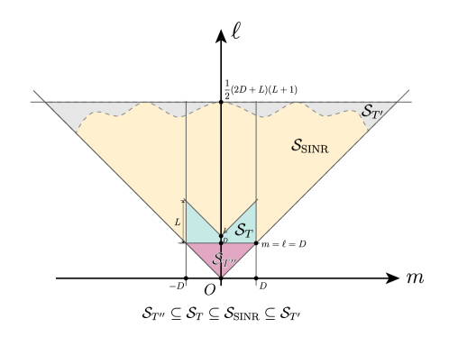
Figure 3: Illustration of the inclusion relationships projected into the spectral modes $(m,\ell)$. Note that the range for $\mathcal{S}_{\textrm{SINR}}$ is only for reference.

By combining the expansion of the SINR architecture and its representability, we can conclude that the SINR architecture acts as a universal approximator on the 2D-sphere with the aid of the linear subspace spanned by the spherical harmonics.

Lemma 3.8 (convergence of Fourier-Laplacian series).

Let $\mathcal{P}_{d}$ be the projection operator onto the space spanned by the spherical harmonics $Y_{\ell}^{m}$ with $|m|\leq\ell=d$, then the Fourier-Laplacian series of $f\in L^{2}(\mathbb{S}^{2})$

$$\sum_{d=0}^{N}\mathcal{P}_{d}f\to f\textrm{ in }L^{2}(\mathbb{S}^{2})\textrm{ as }N\to+\infty,$$ (44)

and the convergence is uniform if $f$ is smooth enough. [6]

Theorem 3.9 (convergence of SINRs).

For any $f\in L^{2}(\mathbb{S}^{2})$,

$$\lim_{D,L\to\infty}\inf_{f^{\prime}\in\mathcal{S}_{\textrm{SINR}}}\|f^{\prime}-f\|_{L^{2}(\mathbb{S}^{2})}=0.$$ (45)

Furthermore, if $f\in C^{\infty}(\mathbb{S}^{2})$,

$$\lim_{D,L\to\infty}\inf_{f^{\prime}\in\mathcal{S}_{\textrm{SINR}}}\|f^{\prime}-f\|_{C(\mathbb{S}^{2})}=0.$$ (46)

Proof.

The proof is a direct consequence of the inclusion $\mathcal{S}_{T^{\prime\prime}}\subseteq\mathcal{S}_{T}\subseteq\mathcal{S}_{\textrm{SINR}}$, where

$$T^{\prime\prime}=\{(m,\ell)\mid|m|\leq\ell\leq\min(D,L)\}$$ (47)

by Corollary 3.7 and Lemma 3.8. ∎

Remark.

Qualitatively speaking, the rate of convergence is tied to the smoothness of the target function $f$. As the degree $D$ and the number of layers $L$ increase, the smoother the function is, the faster $\mathcal{S}_{T^{\prime\prime}}$ converges as well as $\mathcal{S}_{\textrm{SINR}}$. Readers may refer to [6] for detailed discussions. Generally, the uniform convergence is expected since most natural physical fields exhibit smooth behavior.

3.2 Modulation adjustment

Directly treating the network parameters $\bm{W}^{(l)}$, $\bm{b}^{(l)}$, $\tilde{\bm{W}}^{(l)}$ and $\tilde{\bm{b}}^{(l)}$ together with the scalar matrix of the spherical filter for each layer of our SINR architecture (33) as the latent representation $\bm{z}$ can hardly achieve our purpose of efficient reduction of dimensions. Therefore, we propose to use the modulation adjustment, which is also a common technique of most existing INR networks. The idea is to uses a shared base network across different snapshots to model universal physical structure, with modulations modeling the variation specific to individual time steps [61, 52]. Experiments have indicated that a simple modulation shift [25] for each layer is sufficient for our tasks. The modulation adjustment for the SINR architecture (33) is

$$\bm{z}^{(0)} =\bm{g}_{0}(\bm{p}),\qquad\bm{p}\in\mathbb{S}^{2},$$ (48)

$$\bm{z}^{(l)} =\left(\bm{W}^{(l)}\bm{z}^{(l-1)}+\bm{b}^{(l)}+\bm{q}^{(l)}(\bm{z})\right)\odot\bm{g}_{l}(\bm{p}),\quad l=1,2,\cdots,L,$$

$$I(\bm{p};\bm{z},\bm{\varphi}) =\sum_{l=0}^{L}\left(\tilde{\bm{W}}^{(l)}\bm{z}^{(l)}+\tilde{\bm{b}}^{(l)}\right),$$

where $\bm{q}^{(l)}(\bm{z})$ stands for a trainable affine mapping of the latent representation $\bm{z}$ for the $l$-th layer, and the parameters are not shared across different layers. The original weights and biases of the SINR structure as well as the trainable parameters of the modulation adjustment $\bm{q}^{(l)}$ together make up of the optimization variable $\bm{\varphi}$ in (21). Note that only the latent representation $\bm{z}$ varies across different snapshots, while the network parameters $\bm{\varphi}$ remain consistent. Therefore, the dimension of the latent space is reduced to the size of $\bm{z}$. Figure 4 visualizes the detailed structure of a SINR with modulation adjustments.

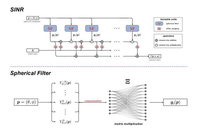
Figure 4: Visualization of the SINR architecture with modulation adjustments and the spherical filters.

3.3 Continuous-time latent surrogate model

To address the challenges posed by temporally uneven distributions of observation data, we model the latent dynamics as a continuous-time dynamical system

$$\frac{\mathrm{d}\bm{z}}{\mathrm{d}t}=\bm{F}(\bm{z})\approx\bm{f}_{\bm{\psi}}(\bm{z})$$ (49)

with the set of trainable parameters denoted by $\bm{\psi}$, and we have chosen the Neural ODE structure [19, 18] for the implementation. It’s worth noting that such structures are suitable for handling time-series data, as they offer a data-efficient way to parameterize a trajectory over time and naturally deal with arbitrary time steps. These advantages make neural ODEs a fitting choice for modeling the latent dynamics in our LAINR framework in that the time steps are usually irregular for realistic assimilation process.

3.4 Modeling of uncertainties

There are in general two types of uncertainty we need to model in the assimilation process. One is the prediction uncertainties of the surrogate model responsible for latent dynamics, which is inevitable due to the very nature of network training. The other is the uncertainty of the latent background estimate, which characterizes the latent uncertainty transformed from the physical background by the encoder mapping. We assume that the encoder mapping is perfect, which mean that the optimization problem (23) is solved with a negligible margin of error. Experimental results have validated the practical effectiveness of such simplification.

3.4.1 Uncertainty estimator for the latent surrogate model

Upon successful training of the latent surrogate model, let $\hat{\bm{z}}_{k+1}=\mathcal{G}(\bm{z}_{k})$ be the predicted latent state at the $(k+1)$-th time step, given the latent state $\bm{z}_{k}$ at $k$-th time step. We model the prediction uncertainty as a Gaussian distribution. To put it formally,

$$\mathcal{G}(\bm{z}_{k})=\hat{\bm{z}}_{k+1}=\bm{z}_{k+1}+\bm{\varepsilon}_{k+1}^{L},\quad\bm{\varepsilon}_{k+1}^{L}\sim\mathcal{N}(0,\bm{\Sigma}^{L}),$$ (50)

where $\bm{\Sigma}^{L}$ is the covariance matrix of the uncertainty $\bm{\varepsilon}_{k+1}^{L}$ of the latent surrogate model $\mathcal{G}$, and we assume it to be time-independent. Our LAINR framework learns the Cholesky decomposition of the uncertainty covariance matrix $\bm{\Sigma}^{L}$, which means that for the Cholesky decomposition

$$\bm{\Sigma}^{L}=\bm{L}\bm{L}^{\mathsf{T}},\textrm{ or equivalently, }(\bm{\Sigma}^{L})^{-1}=\bm{L}^{-\mathsf{T}}\bm{L}^{-1},$$ (51)

where the matrix $\bm{L}$ as well as its inverse $\bm{L}^{-1}$ are both positive-definite lower-triangular matrices. We parameterize the $\bm{L}^{-1}$ as

$$\bm{L}^{-1}=\tilde{\bm{L}}+\exp\bm{D}.$$ (52)

Here, $\tilde{\bm{L}}$ is a lower-triangular matrix with zero diagonal entries, and $\exp\bm{D}$ stands for the element-wise exponential of a diagonal matrix $\bm{D}$ to ensure its positive-definiteness. We refer to the tuple $(\tilde{\bm{L}},\bm{D})$ as our uncertainty estimator for the latent surrogate model hereafter. Both the two matrices $\tilde{\bm{L}}$ and $\bm{D}$ are initialized with zeros and then optimized during training, where the target loss function is derived as follows. With the independence assumption, the likelihood of the uncertainties $\{\bm{\xi}_{k}\}_{k}$ across the whole dataset reads

$$\mathbb{P}\left(\{\bm{\xi}_{k}\}_{k}\right)=\prod_{k}(2\pi)^{-m/2}\det(\bm{\Sigma}^{z})^{-1/2}\exp\left(-\frac{1}{2}\left(\mathcal{G}(\bm{z}_{k})-\bm{z}_{k+1}\right)^{\mathsf{T}}(\bm{\Sigma}^{z})^{-1}\left(\mathcal{G}(\bm{z}_{k})-\bm{z}_{k+1}\right)\right).$$ (53)

Consequently, we adjust the uncertainty estimator $(\tilde{\bm{L}},\bm{D})$ by minimizing the negative log-likelihood

$$\mathcal{L}_{\textrm{MLE}} =\sum_{k}\frac{1}{2}\log\det(\bm{\Sigma}^{z})+\frac{1}{2}\left(\mathcal{G}(\bm{z}_{k})-\bm{z}_{k+1}\right)^{\mathsf{T}}(\bm{\Sigma}^{z})^{-1}\left(\mathcal{G}(\bm{z}_{k})-\bm{z}_{k+1}\right)$$ (54)

$$=\sum_{k}\log\det\bm{L}+\frac{1}{2}\left(\mathcal{G}(\bm{z}_{k})-\bm{z}_{k+1}\right)^{\mathsf{T}}\bm{L}^{-\mathsf{T}}\bm{L}^{-1}\left(\mathcal{G}(\bm{z}_{k})-\bm{z}_{k+1}\right)$$

$$=\sum_{k}\left(-\sum_{j}\bm{D}_{jj}\right)+\frac{1}{2}\left\|\bm{L}^{-1}\left(\mathcal{G}(\bm{z}_{k})-\bm{z}_{k+1}\right)\right\|^{2}$$

up to a constant by the method of maximum likelihood estimation (MLE), where the outer summation runs through all the latent representations $\bm{z}_{k}$, and the inner summation $\sum_{j}\bm{D}_{jj}$ represents the sum of the diagonal entries of $\bm{D}$.

3.4.2 Uncertainty of the latent background estimate

Consider a physical background estimate

$$\bm{x}_{0}^{b}=\bm{x}_{0}+\bm{\varepsilon}_{x}^{b},\quad\bm{\varepsilon}_{x}^{b}\sim\mathcal{N}(0,\bm{\Sigma}_{x}^{b})$$ (55)

given as a Gaussian perturbation of the true physical state $\bm{x}_{0}$. The encoder mapping $\mathcal{E}$ transforms it into a latent background estimate

$$\bm{z}_{0}^{b}=\mathcal{E}\left(\bm{x}_{0}^{b}\right)=\mathcal{E}\left(\bm{x}_{0}+\bm{\varepsilon}_{x}^{b}\right)=\mathcal{E}\left(\bm{x}_{0}\right)+\bm{J}_{\mathcal{E}}(\bm{x}_{0})\bm{\varepsilon}_{x}^{b}+o\left(\bm{\varepsilon}_{x}^{b}\right)=\bm{z}_{0}+\bm{J}_{\mathcal{E}}(\bm{x}_{0})\bm{\varepsilon}_{x}^{b}+o\left(\bm{\varepsilon}_{x}^{b}\right),$$ (56)

where $\bm{J}_{\mathcal{E}}$ is the Jacobian matrix of $\mathcal{E}$. By omitting the high-order term, we make the following approximation

$$\bm{z}_{0}^{b}\approx\bm{z}_{0}+\bm{J}_{\mathcal{E}}(\bm{x}_{0})\bm{\varepsilon}_{x}^{b}=\bm{z}_{0}+\bm{\varepsilon}_{z}^{b},\quad\bm{\varepsilon}_{z}^{b}\sim\mathcal{N}\left(0,\bm{J}_{\mathcal{E}}(\bm{x}_{0})\bm{\Sigma}_{z}^{b}\bm{J}_{\mathcal{E}}(\bm{x}_{0})^{\mathsf{T}}\right).$$ (57)

Since the encoder mapping $\mathcal{E}$ is associated with an optimization process, no explicit formula for the Jacobian matrix $\bm{J}_{\mathcal{E}}$ is available. Therefore, we choose to make use of the decoder mapping $\mathcal{D}$ in that the chain rule gives

$$\bm{J}_{\mathcal{E}}(\bm{x}_{0})\bm{J}_{\mathcal{D}}(\bm{z}_{0})=\bm{J}_{\mathcal{E}}(\mathcal{D}(\bm{z}_{0}))\bm{J}_{\mathcal{D}}(\bm{z}_{0})=\bm{J}_{\mathcal{E}\circ\mathcal{D}}(\bm{z}_{0})=\bm{I}_{m}.$$ (58)

First, for any physical background estimate $\bm{x}_{0}^{b}$, LAINR calculates the latent background estimate $\bm{z}_{0}^{b}=\mathcal{E}(\bm{x}_{0}^{b})$. It follows that the Jacobian $\bm{J}_{\mathcal{D}}(\bm{z}_{0})$ is approximated by $\bm{J}_{\mathcal{D}}(\bm{z}_{0}^{b})$ with the aid of automatical differentiation on the decoder mapping $\mathcal{D}$. The Moore-Penrose inverse of $\bm{J}_{\mathcal{D}}(\bm{z}_{0}^{b})$ is used to approximate $\bm{J}_{\mathcal{E}}(\bm{x}_{0})$ afterwards in that they are both the left inverse of $\bm{J}_{\mathcal{D}}(\bm{z}_{0}^{b})$, which is then employed to construct the covariance matrix $\bm{J}_{\mathcal{E}}(\bm{x}_{0})\bm{\Sigma}_{z}^{b}\bm{J}_{\mathcal{E}}(\bm{x}_{0})^{\mathsf{T}}$ for $\bm{\varepsilon}_{z}^{b}$.

3.5 The proposed LAINR framework

LAINR shares some similarities with the LA framework described in Section 2.3. It requires observed data $\{\bm{y}_{k}\}_{k}$, observation operators $\{\mathcal{H}_{k}\}_{k}$ and a background estimate $\bm{x}_{0}$ to initiate the assimilation process. In contrast to the LA framework, any ungridded historical dataset encoding the physical dynamics is sufficient for LAINR to obtain a latent surrogate model for the dynamics, and LAINR additionally provides the corresponding uncertainty estimations for the trained networks. The overall procedure for the deployment of our LAINR framework is summarized as follows.

1. Train the encoder-decoder mappings implemented via the SINR architecture as detained in Section 3.1 with (21). The resulting encoder $\mathcal{E}:\mathcal{X}^{\prime}\to\mathcal{Z}$ and decoder $\mathcal{D}:\mathcal{Z}\to\mathcal{X}^{\prime}$ are given by (23)(22). Besides, the latent surrogate model $\mathcal{G}:\mathcal{Z}\to\mathcal{Z}$ is implemented via Neural ODE (Section 3.3) such that

   $$\mathcal{D}\circ\mathcal{E}\approx\textrm{identity mapping on }\mathcal{X}^{\prime};\qquad\mathcal{D}\circ\mathcal{G}\circ\mathcal{E}\approx\mathcal{M}.$$ (59)

   In other words, the encoder $\mathcal{E}$ and the decoder $\mathcal{D}$ are inverse mappings such that the diagram in Figure 2 (b) commutes up to a small error.

2. Use the uncertainty estimator to evaluate the uncertainty covariance matrix $\bm{\Sigma}^{z}$ for the latent surrogate model $\mathcal{G}$. The uncertainty estimator is trained by the method of maximum likelihood estimation (MLE) using the latent representations of the training dataset $\{\bm{z}_{k}\}_{k}$. (Section 3.4.1)

3. Determine the latent background estimate $\bm{z}_{0}^{b}=\mathcal{E}(\bm{x}_{0}^{b})$ and calculate its associated uncertainty covariance matrix. (Section 3.4.2)

4. Implement the assimilation process on the latent space with an existing well-developed DA algorithm, where $\mathcal{G}$ serves as the latent forward propagation operator and $\mathcal{H}^{\prime}=\mathcal{H}\circ\mathcal{D}$ acts as the observation operator. The observation noise of $\mathcal{H}^{\prime}=\mathcal{H}\circ\mathcal{D}$ remains the same as that of $\mathcal{H}$. The uncertainty estimations are given in the previous two steps.

5. Retrieve the assimilated system states $\left\{\bm{x}_{k}^{a}\right\}_{k}$ from their assimilated latent representations via the decoder $\bm{x}_{k}^{a}=\mathcal{D}(\bm{z}_{k}^{a})$.

4 Experiments

To assess the scalability of our proposed LAINR framework, we choose multi-dimensional partial differential equations (PDEs) as our test cases instead of chaotic ordinary differential equations (ODEs) like the Lorenz-96 model adopted in the previous works [62, 60]. The reason is that PDEs typically possess a much higher-dimensional state space compared to ODEs, thus providing a more rigorous test of scalability. For this study, both the ideal shallow-water model as well as the more realistic ERA5 reanalysis data have been established as the test cases in this paper.

It is also important to mention that our framework aims to handle unknown dynamics, and only partial physical features are used to build the encoder-decoder mappings and the latent surrogate model. Although LAINR has the flexibility to work with diverse types of sampling sets with little adjustment, we still use gridded dataset in order to make fair comparison with the existing AutoEncoder-based methodologies. The appliability of our LAINR framework for inconsistent sampling sets is further demonstrated in the last subsection.

4.1 Test cases

4.1.1 The shallow-water equation

Consider the following spherical shallow-water equation on the 2D sphere

$$\frac{\mathrm{d}\bm{u}}{\mathrm{d}t} =-f\bm{k}\times\bm{u}-g\nabla h+\nu\Delta\bm{u},$$ (60)

$$\frac{\mathrm{d}h}{\mathrm{d}t} =-h\nabla\cdot\bm{u}+\nu\Delta h,$$

with the material derivative denoted by $\frac{\mathrm{d}}{\mathrm{d}t}$. The vorticity field $w=\nabla\times\bm{u}$ together with the thickness of the fluid layer $h$ becomes the system states to be assimilated. $\nu$ stands for the diffusion parameter, and the parameters $f$, $g$, $\Omega$ are all fixed and in consistent with the real earth surface. The model is set up by initialize two symmetric zonal flow representing typical mid-latitude tropospheric jets, and the initial thickness $h$ involves solving a boundary-value problem (balanced equation) [31]. The maximal zonal wind varies in order to create 20 different trajectories for training and testing purposes. All the trajectories have been generated and recorded within a $128\times 64$ regular lat-lon grid with $\Delta t\approx 1$ real hour. See B.1 for detailed configurations.

4.1.2 ERA5 datasets

ERA5 datasets [35] are the latest global atmospheric reanalysis datasets produced by the European Centre for Medium-Range Weather Forecasts (ECMWF), which are generated by assimilating observations from across the world into a delicate numerical weather prediction model. In our experiments, we do not make comparison with the DA algorithms employed in the generation of ERA5 datasets, but treat the datasets as the ground truth to provide a more realistic model than the ideal shallow-water model.

We extract both the Z500 (geopotential at 500 hPa) and the T850 (temperature at 850 hPa) fields from the WeatherBench [65] dataset, which is a resampled version of the ERA5 datasets specially designed for DL training. The choice of Z500 and T850 aligns with those of the early attempts [23, 68, 78, 66] of DL-based weather forecasting. The Z500 and T850 fields are used to train the surrogate models, which are also the physical features we aim to assimilate. Similar to the configurations of the shallow-water model, the spatial resolution of the Z500 and T850 fields are $128\times 64$ ($2.8125^{\circ}\times 2.8125^{\circ}$) with $\Delta t=1$ hour. The data are collected within 10 years ranging from 2009 to 2018.

4.2 Model configurations and training process

4.2.1 Encoder-decoder mappings

AutoEncoder

In the previous work [62], the encoder-decoder mappings have been implemented with fully-connected neural networks. Nevertheless, such design choice raises potential scalability issues for our two-dimensional test cases, considering the prohibitively large parameter volume. Directly applying fully-connected networks could lead to a parameter volume of roughly $(2\times 128\times 64)^{2}\times d\approx 2.7\times 10^{8}\times d$ for a network of depth $d$ with 2-channel input of size $128\times 64$, which is impractical, particularly as this volume grows with the scale of the real deployment. Consequently, to make a systematical comparison with the AutoEncoder-based LA framework and circumvent the scalability concerns, we have opted to leverage convolutional neural networks (CNNs) to establish our baselines. The decision aligns with the natural suitability of CNNs for tasks that exhibit local spatial or temporal correlations.

We have chosen the Convolutional AutoEncoder (CAE) structure as employed in [1] for assimilating the room $\textrm{CO}_{2}$ concentration, and the AEflow [32] structure proposed in the field of turbulent flow simulation. With the latent dimension fixed, we vary the kernel size $K\in\{3,5,7\}$ and the number of hidden channels $C\in\{8,16,32\}$ for the CAE structure, and the kernel size $K\in\{3,5,7\}$ and the number of residual blocks $N_{\textrm{res}}\in\{4,8,12\}$ for the AEflow structure. To make the convolutions compatible with the boundary condition, we utilize periodic paddings along the zonal directions and replication paddings at the poles. See Appendix C.1 for detailed descriptions.

INR

As introduced in Section 3.1, we have chosen the SINR structure as our INR implementation due to its reliable convergence guarantee. By empirically tuning the hyperparameters, we fix the hidden dimensions $h=384$ and $D=L=8$ for our implementation of SINR in the following experiments.

4.2.2 Surrogate model for latent dynamics

Discrete-time dynamical system

We follow the work of [62] and implement the surrogate model for the latent dynamics with the ReZero structure [7] as a discrete-time dynamical model. The ReZero structure is implemented with 5 residual blocks, and the activation function is fixed as the LeakyReLU [51] except for the final block.

Continuous-time dynamical system

As explained in Section 3.3, we choose to use the Neural ODE architecture with the surrogate model implemented via a fully-connected network. The network is trained with an RK4 integrator via TorchDiffEq [19, 18] package based on PyTorch [57].

4.2.3 Metrics

To show the advantages of our LAINR framework, we choose three different sets of methods for our experiments as detailed in Table 3. Note that all the methods are trained with identical training dataset and then evaluated on a separated testing dataset. In the literatures, the performances are usually quantified by the rooted-mean-square error $\operatorname{\mathcal{L}^{\mathrm{skip}}}$ on the quasi-uniform skipped latitude-longitude grid $G_{\mathrm{skip}}$ [77] or the weighted rooted-mean-square error $\operatorname{\mathcal{L}^{\mathrm{weighted}}}$ with respect to the cosine values of latitudes, formulated as

$$\operatorname{\mathcal{L}^{\mathrm{skip}}}(\bm{x},\bm{x}^{\prime}) =\sqrt{\frac{1}{|G\cap G_{\mathrm{skip}}|}\sum_{\bm{p}\in G\cap G_{\mathrm{skip}}}\left\|\bm{x}(\bm{p})-\bm{x}^{\prime}(\bm{p})\right\|^{2}},$$

$$\operatorname{\mathcal{L}^{\mathrm{weighted}}}(\bm{x},\bm{x}^{\prime}) =\sqrt{\frac{1}{\sum_{\bm{p}\in G}\cos\phi(\bm{p})}\sum_{\bm{p}\in G}\left\|\bm{x}(\bm{p})-\bm{x}^{\prime}(\bm{p})\right\|^{2}\cos\phi(\bm{p})},$$

where $\phi(\bm{p})$ is evaluated as the latitude of the position $\bm{p}$, the networks parameters are trained to minimize the same corresponding discrepancy. No significant differences between these two metrics have been found throughout our experiments (not shown), so we fix the metric for both training and evaluation as the weighted rooted-mean-square error $\operatorname{\mathcal{L}^{\mathrm{weighted}}}$ and then omit the supscripts in that it is more compatible with the $L^{2}$ norm and more flexible when applied to ungridded data.

4.2.4 Training process

All the network parameters are optimized with the Adam optimizer [39], but the training processes for AutoEncoders and SINRs are slightly different concerning the stability of training. The training of the AutoEncoder baselines follows [62], which optimize a linear combination of the recovery loss

$$L_{\textrm{rec}}^{\textrm{AE}}(\bm{x})=\mathcal{L}(\bm{x},\mathcal{D}\circ\mathcal{E}(\bm{x}))$$ (61)

and the prediction loss

$$L_{\textrm{pred}}^{\textrm{AE}}(\bm{x}_{k})=\mathcal{L}(\bm{x}_{k+1},\mathcal{D}\circ\mathcal{G}\circ\mathcal{E}(\bm{x}_{k})).$$ (62)

As for our proposed LAINR framework, the encoder-decoder mappings are only updated for each epoch. The latent representations are trained together with the parameters of the encoder with the recovery loss

$$L_{\textrm{rec}}^{\textrm{INR}}(\bm{x},\bm{z})=\mathcal{L}(\bm{x},\mathcal{D}(\bm{z})).$$ (63)

Instead of optimizing the prediction loss (62), we apply the exponential Scheduled Sampling [10] with the multi-step-ahead prediction loss on the latent space

$$L_{\textrm{pred}}^{\textrm{INR},(s)}(\bm{z}_{k})=\|\bm{z}_{k+s}-\mathcal{G}^{s}(\bm{z}_{k})\|^{2}.$$ (64)

For each model, we first pre-train it without updating the latent surrogate model to make it focus on obtaining a good latent embeddings for all the snapshots. Then the model is fine-tuned with both the recovery loss and the prediction loss to reconstruct the latent dynamics. The detailed training processes for the AutoEncoder and the INR models are summarized in Algorithm 1 and Algorithm 2, respectively, where we demostrate the optimization with Stochastic Gradient Descent (SGD) with a consistent learning rate $\eta$ for simplicity.

Algorithm 1 Training for AutoEncoder

1:  Input: Training data $\{\bm{x}_{k}\}_{k}$, epochs $T$

2:  Output: trained models $\mathcal{E}_{\bm{\theta}}$, $\mathcal{D}_{\bm{\varphi}}$, $\mathcal{G}_{\bm{\psi}}$

3:  Initialize $\mathcal{E}_{\bm{\theta}}$, $\mathcal{D}_{\bm{\varphi}}$ and $\mathcal{G}_{\bm{\psi}}$.

4:  for $t=1$ to $T$ do

5:      for $\bm{x}_{k}$ in $\{\bm{x}_{k}\}_{k}$ do

6:         ** forward propagation **

7:         Calculate the recovery loss $L_{\textrm{rec}}^{\textrm{AE}}(\bm{x}_{k})$;

8:         Calculate the prediction loss $L_{\textrm{pred}}^{\textrm{AE}}(\bm{x}_{k})$;

9:         ** update weights **

10:         $\bm{\theta}\leftarrow\bm{\theta}-\eta\nabla_{\bm{\theta}}\left(L_{\textrm{rec}}^{\textrm{AE}}+L_{\textrm{pred}}^{\textrm{AE}}\right)$

11:         $\bm{\varphi}\leftarrow\bm{\varphi}-\eta\nabla_{\bm{\varphi}}\left(L_{\textrm{rec}}^{\textrm{AE}}+L_{\textrm{pred}}^{\textrm{AE}}\right)$

12:         $\bm{\psi}\leftarrow\bm{\psi}-\eta\nabla_{\bm{\psi}}L_{\textrm{pred}}^{\textrm{AE}}$

13:      end for

14:  end for

Algorithm 2 Training for INR

1:  Input: Training data $\{\bm{x}_{k}\}_{k}$, epochs $T$

2:  Output: trained models $\mathcal{D}_{\bm{\varphi}}$, $\mathcal{G}_{\bm{\psi}}$

3:  Initialize $\mathcal{D}_{\bm{\varphi}}$, $\mathcal{G}_{\bm{\psi}}$ and $\{\bm{z}_{k}\}_{k}$.

4:  for $t=1$ to $T$ do

5:      for $\bm{x}_{k}$ in $\{\bm{x}_{k}\}_{k}$ do

6:         ** train the encoder-decoder **

7:         Calculate the recovery loss $L_{\textrm{rec}}^{\textrm{INR}}(\bm{x}_{k},\bm{z}_{k})$;

8:         ** update only the latent vectors **

9:         $\bm{z}_{k}\leftarrow\bm{z}_{k}-\eta\nabla_{\bm{z}_{k}}L_{\textrm{rec}}^{\textrm{INR}}(\bm{x}_{k},\bm{z}_{k})$

10:         Calculate the prediction loss $L_{\textrm{pred}}^{\textrm{INR,(s)}}(\bm{z}_{k})$;

11:      end for

12:      ** update model weights **

13:      $\bm{\varphi}\leftarrow\bm{\varphi}-\eta\nabla_{\bm{\varphi}}\sum_{k}L_{\textrm{rec}}^{\textrm{INR}}(\bm{x}_{k},\bm{z}_{k})$

14:      $\bm{\psi}\leftarrow\bm{\psi}-\eta\nabla_{\bm{\psi}}\sum_{k}L_{\textrm{pred}}^{\textrm{INR},(s)}(\bm{z}_{k})$

15:  end for

16:  ** output the encoder **

17:  the encoder $\mathcal{E}$ is given implicitly as follows:

18:  $\bm{x}\mapsto\bm{z}=\operatorname*{argmin}_{\bm{z}^{\prime}}\mathcal{L}(\bm{x}_{k},\mathcal{D}_{\bm{\varphi}}(\bm{z}^{\prime}))$.

method name	encoder/decoder	latent dynamics	latent dimension
CAE-ReZero	CAE [1]	ReZero [7]	1024
AEflow-ReZero	AEflow [32]	ReZero [7]	1024
LAINR (ours)	SINR (Section 3.1)	Neural ODE [19, 18]	400

Table 3: Different methods for comparison in the experiments.

4.3 Performance comparisons

4.3.1 Exploring low-dimensional representations

Our experiments start with an exploration of the underlying linear low-dimensional structure within the datasets, followed by a comparative analysis of the reconstruction capabilities of the three distinct ROMs: CAE, AEflow and SINR. The assessment has been conducted independently of the surrogated model assigned to handle latent dynamics, which means only the encoder-decoder mappings are trained.

First, after computing the empirical covariance matrix for all the snapshots within the training dataset, we calculate all the eigenvalues and corresponding eigenvectors for the matrix $\bm{X}\bm{X}^{\mathsf{T}}$ as defined in Section 2.1.1 and then sort the eigenvalues in descending order. As illustrated in Figure 5, 1000 dominant modes encode most of the physical features for the shallow-water model well, but as real physical states grow much more complex, the ERA5 data cannot be recovered accurately with less than 4000 modes. We decide to set the latent dimension for the baselines (CAE and AEflow) as 1024 that of our LAINR framework as 400 (See Table 3), which present a more challenging setup to explore their generalizability.

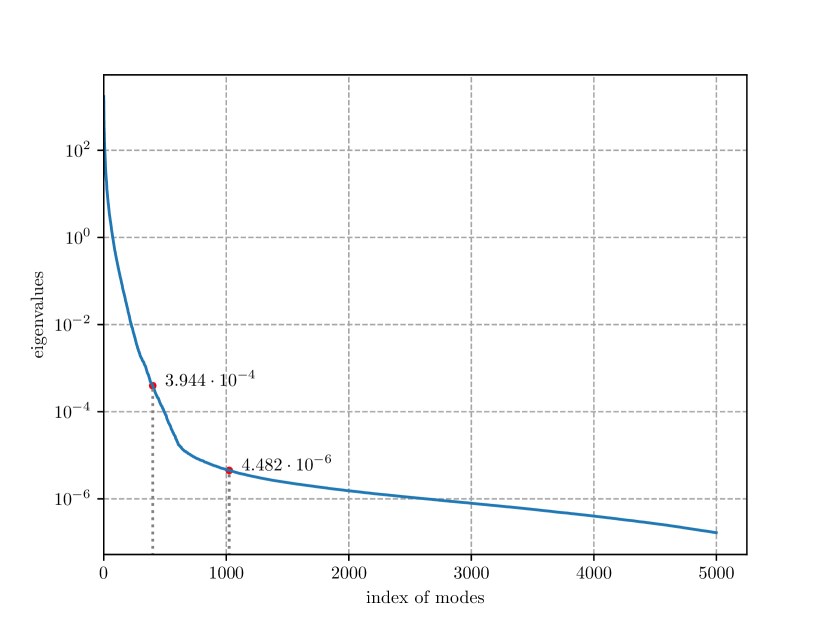
(a) shallow-water model

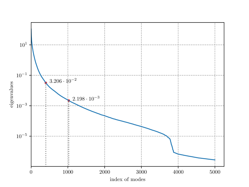
(b) ERA5 data

Figure 5: Distributions of the 5000 largest eigenvalues of the covariance matrix. The 400-th and the 1024-th eigenvalues are marked on the graph.

For each method, we have recorded the reconstruction error on the training dataset and subsequently evaluated its generalization ability on a separate testing dataset. Furthermore, for the previous CAE and AEflow architectures, we conduct a grid search (Appendix C.2) on the configurations for the optimal network structures based on the following averaged reconstruction error

$$L_{\mathrm{rec}}=\frac{1}{N}\sum_{k=1}^{N}\operatorname{\mathcal{L}^{\mathrm{weighted}}}(\bm{x}_{k},\mathcal{D}\circ\mathcal{E}(\bm{x}_{k}))$$ (65)

between the system states and the recovered strategies, where $k$ refers to the index of each snapshot and $N$ is the total amount. Then we fix the hyperparameters for the following experiments to make a fair comparison with our proposed framework.

When comparing to the AutoEncoder baselines, it is important to note that the two AutoEncoder structures CAE and AEflow both use 1024 dimensions in their latent space. The reconstruction errors for both the training and testing processes are summarized in Figure 6, where the numbers of latent dimensions are appended to the method names. Even with a higher latent dimension, the AutoEncoder methods have shown relatively larger reconstruction errors in both training and testing stages, indicating its inefficiency in capturing and restoring the physical features when the latent dimensionality is limited. In contrast, our SINR architecture operates on a more compressed latent space of merely 400 dimensions, which is less than half of what is utilized by the AutoEncoders, but it still achieves superior performances. Upon observing the compelling accuracy and efficiency of the encoder-decoder mappings implemented via SINR, it becomes clear that our choice of SINR is well-justified.

(a) shallow-water model

(b) ERA5 dataset

Figure 6: Comparison of different structures for dimension reduction

4.3.2 Embedding the physical dynamics

Embedding a physical dynamical system into a latent space involves not only a precise encoding of the snapshot at each time step, but also an accurate discovery of the latent dynamics, which is neccessary for the assimilation process in the latent space. To evaluate both the consistency and the stability of the surrogate models for latent dynamics, the multi-step prediction error

$$L_{\mathrm{pred}}^{(s)}=\frac{1}{N}\sum_{k=1}^{N}\operatorname{\mathcal{L}^{\mathrm{weighted}}}(\bm{x}_{k+s},\mathcal{D}\circ\mathcal{G}^{s}\circ\mathcal{E}(\bm{x}_{k}))$$ (66)

is employed, where $k$ is the time index for the state $\bm{x}$ and $s$ indicates the number of prediction steps. Figure 7 records the increase in prediction errors with respect to the number of predicting steps $s$.

For the shallow-water dataset, both CAE-ReZero and AEflow-ReZero demonstrate comparable performances, while LAINR exhibits significantly lower prediction errors. For the ERA5 dataset, LAINR continues to maintain superior accuracy, but the prediction errors for the AutoEncoder baselines increase dramatically. Besides, the rate at which prediction errors increase for the AutoEncoder methods is substantially higher than that of LAINR. This observation indicates that our LAINR framework provides enhances stability and more faithful representation of the underlying latent dynamics.

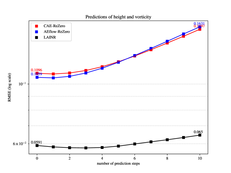
(a) shallow-water dataset

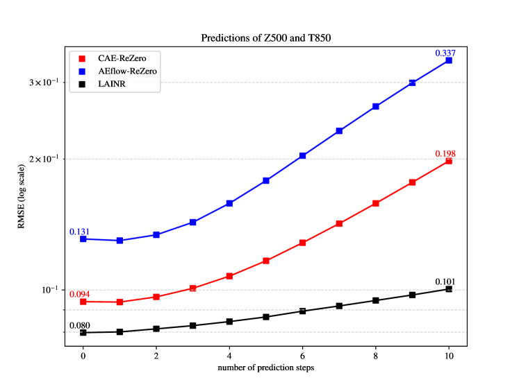
(b) ERA5 dataset

Figure 7: Comparison of multi-step prediction error for different methods on the testing dataset

4.3.3 Compatibility with existing DA algorithms

The effectiveness for a DA algorithm is linked to the quality of the forward integrator, but an accurate surrogate model alone does not guarantee better assimilation performance, owing to the potential incompatibility between the surrogate model’s non-lineality behaviors and the assimilation algorithms. To address such concern, we check the compatibility of our LAINR framework, alongside the AutoEncoder baselines, when paired with existing assimilation algorithms.

We choose several variants of the Kalman filter method for testing, and we would like to emphasize that similar experiments can be extended to other types of assimilation algorithms including the variational methods. Detailed implementations for the associated Kalman filter (KF) algorithms (EnKF, SEnKF, DEnKF, ETKF, ETKF-Q) that involve in our experiments are all exhibited in D.

We set the observation operator as a random sampling on the grid $G$ of size $128\times 64\times 2$ as illustrated in Figure 12 (a) with the number of the observations $n_{\mathrm{obs}}=1024$ (6.25% of the total number of grid points). All observations are perturbed with independent Gaussian noise of variance $(\sigma^{o})^{2}=0.1^{2}$, which is approximately $10\%$ of the ground truth since the datasets are normalized to zero mean and standard deviation in advance. Additionally, the noise for the latent surrogate model is assumed as Gaussian of covariance matrix $(\sigma_{z})^{2}\bm{I}_{m}$. The initial physical background estimate is set as a perturbation of the ground truth evaluated on $G$ with a Gaussian noise $\sigma_{x}^{b}=0.1$, and the covariance for the uncertainty of the latent background estimate is set as $(\sigma_{z}^{b})^{2}\bm{I}_{m}$. Both $\sigma_{z}^{b}$ and $\sigma_{z}$ are tuned empirically. See Table 4, 5 and 6 for assimilation results on the shallow-water dataset and Table 7, 8 and 9 for assimilation results on the ERA5 dataset, which list the Rooted Mean Square Errors (RMSEs) across the first 200 assimilation steps in the test datasets. The DA cycle are conducted for each time step. Note that the symbol “-” is marked whenever the assimilation diverges.

Table 4: Comparison of RMSEs for different filters for the CAE-ReZero model on the shallow-water dataset.

$\sigma^{m}$	$\sigma_{z}^{b}$	EnKF	SEnKF	DEnKF	ETKF	ETKF-Q
1.0	$0.1\sigma_{x}^{b}$	1.212	1.643	1.181	1.083	1.516
0.3	$0.1\sigma_{x}^{b}$	1.433	2.256	1.401	1.362	1.619
0.1	$0.1\sigma_{x}^{b}$	1.743	2.396	1.666	1.624	1.656
0.03	$0.1\sigma_{x}^{b}$	1.800	2.413	1.702	1.805	1.666
0.01	$0.1\sigma_{x}^{b}$	1.695	2.414	1.704	1.833	1.683
1.0	$0.01\sigma_{x}^{b}$	1.184	1.643	1.192	1.108	1.631
0.3	$0.01\sigma_{x}^{b}$	1.453	2.256	1.416	1.368	1.637
0.1	$0.01\sigma_{x}^{b}$	1.722	2.396	1.667	1.638	1.440
0.03	$0.01\sigma_{x}^{b}$	1.781	2.413	1.701	1.806	1.527
0.01	$0.01\sigma_{x}^{b}$	1.715	2.414	1.703	1.838	1.602

Table 5: Comparison of RMSEs for different filters for the AEflow-ReZero model on the shallow-water dataset.

$\sigma^{m}$	$\sigma_{z}^{b}$	EnKF	SEnKF	DEnKF	ETKF	ETKF-Q
1.0	$0.1\sigma_{x}^{b}$	0.7958	0.8265	0.7332	0.7313	1.179
0.3	$0.1\sigma_{x}^{b}$	0.7290	1.016	0.7551	0.7473	1.195
0.1	$0.1\sigma_{x}^{b}$	0.8232	1.282	0.8196	0.8378	1.161
0.03	$0.1\sigma_{x}^{b}$	1.0460	1.370	1.028	1.011	1.163
0.01	$0.1\sigma_{x}^{b}$	1.1740	1.378	1.152	1.162	1.214
1.0	$0.01\sigma_{x}^{b}$	0.7967	0.8265	0.7388	0.7303	1.163
0.3	$0.01\sigma_{x}^{b}$	0.7335	1.016	0.7560	0.7517	1.180
0.1	$0.01\sigma_{x}^{b}$	0.8188	1.282	0.8176	0.8405	1.131
0.03	$0.01\sigma_{x}^{b}$	1.042	1.370	1.031	1.013	1.111
0.01	$0.01\sigma_{x}^{b}$	1.171	1.378	1.151	1.161	1.014

Table 6: Comparison of RMSEs for different filters for LAINR (ours) on the shallow-water dataset. The last row indicates the assimilation RMSEs when the uncertainty estimator is used.

$\sigma^{m}$	$\sigma_{z}^{b}$	EnKF	SEnKF	DEnKF	ETKF	ETKF-Q
0.01	$0.1\sigma_{x}^{b}$	0.08746	0.08582	0.08564	0.09012	0.05559
0.003	$0.1\sigma_{x}^{b}$	0.06414	0.07804	0.05998	0.06478	0.05394
0.001	$0.1\sigma_{x}^{b}$	0.05556	0.07999	0.05408	0.05690	0.05335
0.0003	$0.1\sigma_{x}^{b}$	0.05781	0.08564	0.05227	0.05451	0.05372
0.0001	$0.1\sigma_{x}^{b}$	0.05759	0.08814	0.05834	0.05487	0.05505
0.01	$0.01\sigma_{x}^{b}$	0.08746	0.08582	0.08563	0.09013	0.06535
0.003	$0.01\sigma_{x}^{b}$	0.06413	0.07804	0.05998	0.06477	0.06290
0.001	$0.01\sigma_{x}^{b}$	0.05549	0.08002	0.05400	0.05690	0.05334
0.0003	$0.01\sigma_{x}^{b}$	0.05760	0.08569	0.05221	0.05455	0.05318
0.0001	$0.01\sigma_{x}^{b}$	0.05686	0.08820	0.05750	0.05484	0.05532
uncertainty estimator		0.05534	0.08648	0.05225	0.05404	0.05888

Table 7: Comparison of RMSEs for different filters for the CAE-ReZero model on the ERA5 dataset.

$\sigma^{m}$	$\sigma_{z}^{b}$	EnKF	SEnKF	DEnKF	ETKF	ETKF-Q
1.0	$0.1\sigma_{x}^{b}$	1.900e+3	2.183e+4	274.1	-	3.281
0.3	$0.1\sigma_{x}^{b}$	55.95	2.651e+4	86.64	58.53	5.047
0.1	$0.1\sigma_{x}^{b}$	49.05	2.468e+4	19.91	23.67	5.137
0.03	$0.1\sigma_{x}^{b}$	18.99	2.497e+4	8.201	9.494	5.582
0.01	$0.1\sigma_{x}^{b}$	9.296	2.503e+4	5.435	7.517	5.961
1.0	$0.01\sigma_{x}^{b}$	5.831e+3	2.704e+4	317.2	-	5.232
0.3	$0.01\sigma_{x}^{b}$	110.0	2.796e+4	79.84	55.06	5.247
0.1	$0.01\sigma_{x}^{b}$	37.17	2.477e+4	19.77	24.26	5.159
0.03	$0.01\sigma_{x}^{b}$	23.57	2.494e+4	8.093	9.322	5.681
0.01	$0.01\sigma_{x}^{b}$	9.002	2.495e+4	6.040	7.459	6.151

Table 8: Comparison of RMSEs for different filters for the AEflow-ReZero model on the ERA5 dataset.

$\sigma^{m}$	$\sigma_{z}^{b}$	EnKF	SEnKF	DEnKF	ETKF	ETKF-Q
1.0	$0.1\sigma_{x}^{b}$	5.507	8.46e+8	5.911	8.149	3.225
0.3	$0.1\sigma_{x}^{b}$	14.08	1.98e+9	11.22	9.714	3.510
0.1	$0.1\sigma_{x}^{b}$	10.99	2.60e+9	9.831	7.522	4.532
0.03	$0.1\sigma_{x}^{b}$	7.092	2.08e+9	5.445	5.827	4.735
0.01	$0.1\sigma_{x}^{b}$	6.908	2.03e+9	5.377	5.987	5.431
1.0	$0.01\sigma_{x}^{b}$	5.526	5.35e+8	6.104	8.072	3.251
0.3	$0.01\sigma_{x}^{b}$	13.52	1.76e+9	11.35	9.675	3.867
0.1	$0.01\sigma_{x}^{b}$	11.71	2.37e+9	9.889	7.500	2.089
0.03	$0.01\sigma_{x}^{b}$	6.862	2.09e+9	5.369	5.847	1.696
0.01	$0.01\sigma_{x}^{b}$	7.210	1.86e+9	5.332	5.967	2.343

Table 9: Comparison of RMSEs for different filters for LAINR (ours) on the ERA5 dataset. The last row indicates the assimilation RMSEs when the uncertainty estimator is used.

$\sigma^{m}$	$\sigma_{z}^{b}$	EnKF	SEnKF	DEnKF	ETKF	ETKF-Q
0.01	$0.1\sigma_{x}^{b}$	0.1881	0.1843	0.1931	0.1835	0.2572
0.003	$0.1\sigma_{x}^{b}$	0.1659	0.1977	0.1778	0.1642	0.2565
0.001	$0.1\sigma_{x}^{b}$	0.1831	0.2613	0.1866	0.1788	0.2558
0.0003	$0.1\sigma_{x}^{b}$	0.2230	0.3056	0.2154	0.2180	0.2559
0.0001	$0.1\sigma_{x}^{b}$	0.2497	0.3147	0.2436	0.2491	0.2571
0.01	$0.01\sigma_{x}^{b}$	0.1883	0.1841	0.1935	0.1827	0.2570
0.003	$0.01\sigma_{x}^{b}$	0.1647	0.1975	0.1774	0.1628	0.2562
0.001	$0.01\sigma_{x}^{b}$	0.1830	0.2604	0.1839	0.1779	0.2556
0.0003	$0.01\sigma_{x}^{b}$	0.2243	0.3036	0.2154	0.2171	0.2556
0.0001	$0.01\sigma_{x}^{b}$	0.2482	0.3121	0.2491	0.2457	0.2578

Notably, LAINR outperforms the AutoEncoder baselines (CAE-ReZero and AEflow-ReZero) with different model noise $\sigma^{m}$ and KF algorithms. Such superior performance of INR emphasizes its robustness across various configurations. The comparison of optimal performances further validates the supremacy of the SINR model. It achieves a considerably lower RMSE than the AutoEncoder methods, reinforcing the idea that the LAINR framework is a superior choice for latent assimilation tasks. Meanwhile, SINR shows its optimal performance with relatively less model noise, demonstrating its higher accuracy in learning the latent dynamics. This aligns with the inherent strengths of the INR approach shown in the previous subsection as well.

By fixing the best configuration for each model, we have visualized the evolution of assimilated system states of the shallow-water dataset along with the ground truth and the differences. See Figure 8, 9 and 10 for the evolution, and Figure 11 for the corresponding assimilation errors for the best configurations displayed in Table 4, 5 and 6. Clearly the AutoEncoder-based methods are unable to capture the physical dynamics during assimilation cycles, and the assimilated states becomes completely noisy within no more than 48 hours. On the contrary, our LAINR approach can keep tracking the dynamics, and the increments for the assimilation error do not grow exponentially.

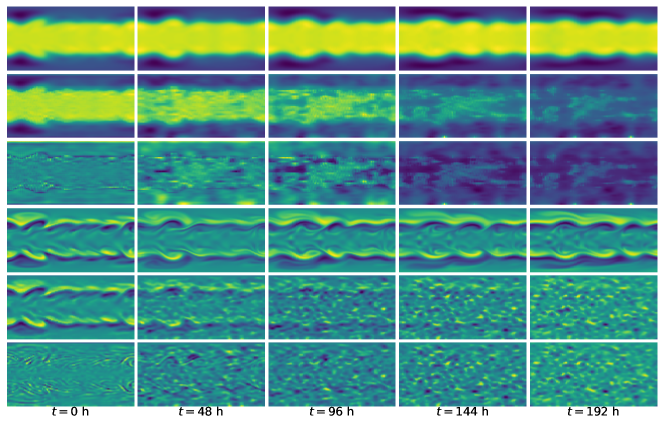
Figure 8: CAE-ReZero with ETKF, $\sigma^{m}=1.0$, $\sigma_{z}^{b}=0.1\sigma_{x}^{b}=0.01$. The first 3 rows and the last 3 rows correspond to the height and the vorticity, respectively. For each feature, the ground truth, the assimilated field as well as the corresponding differences are displayed sequentially.

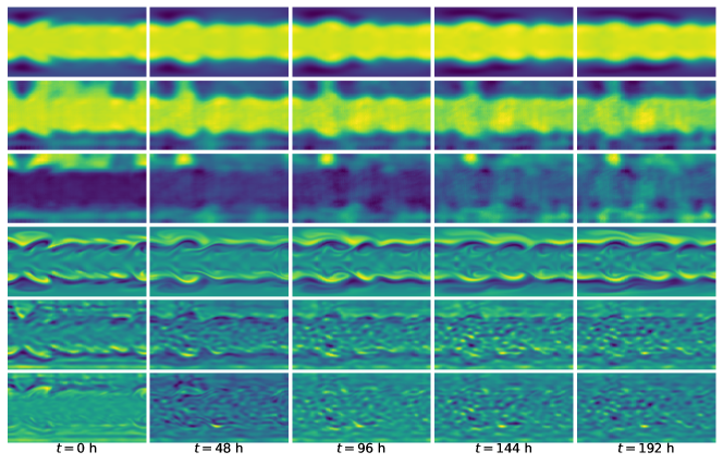
Figure 9: AEflow-ReZero with EnKF, $\sigma^{m}=0.3$, $\sigma_{z}^{b}=0.1\sigma_{x}^{b}=0.01$. The first 3 rows and the last 3 rows correspond to the height and the vorticity, respectively. For each feature, the ground truth, the assimilated field as well as the corresponding differences are displayed sequentially.

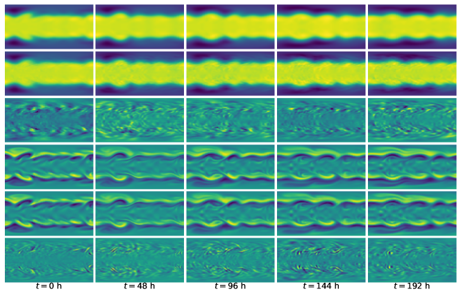
Figure 10: LAINR (ours) with DEnKF, $\sigma^{m}=0.003$, $\sigma_{z}^{b}=0.01\sigma_{x}^{b}=0.001$. The first 3 rows and the last 3 rows correspond to the height and the vorticity, respectively. For each feature, the ground truth, the assimilated field as well as the corresponding differences are displayed sequentially.

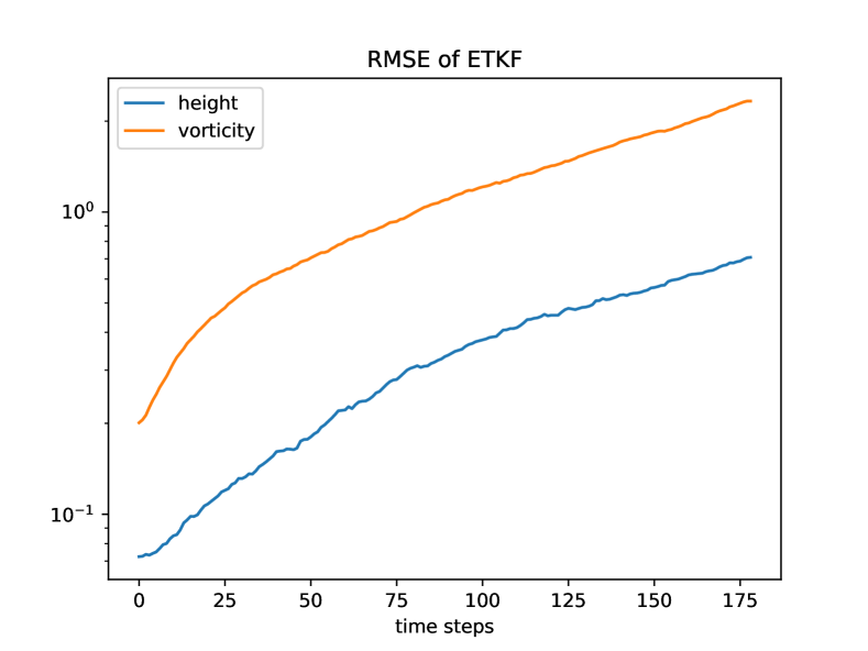
(a) CAE-ReZero with ETKF

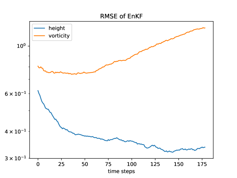
(b) AEflow-ReZero with EnKF

(c) LAINR with DEnKF

Figure 11: Assimilation errors with respect to time steps for the shallow-water dataset

4.3.4 Uncertainty estimations

To study the effectiveness of the uncertainty estimator in our LAINR framework, we have run additional experiments with the model noise and the latent background estimate given as in Section 3.4. The corresponding RMSEs combined with different KF algorithms are attached to Table 6 and Table 9 for both the shallow-water dataset and the ERA5 dataset, respectively. When working with different KF algorithms, the uncertainty estimator serves as a robust method that eliminates the need for empirical tuning of the model noise level $\sigma^{b}$ as well as the uncertainty for the latent background estimate $\sigma_{z}^{b}$. The uncertainty estimator obtains the best performances when coupled with EnKF and ETKF, while it also achieves nearly optimal results across other KF algorithms. It is worth noting that the uncertainty estimator offers an effective data-driven tool to estimate the uncertainties of the trained networks, which can be particularly advantageous in situations where time or computational resources are limited, or where expert knowledge for parameter-tuning is unavailable.

4.4 Offgrid assimilation

Previous experiments are all based on the same regular lat-lon grid for both training and testing to make comparisons with AutoEncoder baselines. To emphasize the flexibility that our proposed LAINR framework can be applied to arbitrary sampling point for inputs, we perform the same assimilation procedure but on a different staggered grid. Figure 12 (b) illustrated the grid $G$ (black) for the network training and the staggered grid $G^{\prime}$ (black) for assimilation. Once the encoder-decoder mappings as well as the surrogate model for latent dynamics has been trained on the grid $G$, we apply LAINR to assimilate the observations on the grid $G^{\prime}$. For this experiment, no observations from $G$ used for training are provided, and only random observations from a subset of $G^{\prime}$ are available for the assimilation process.

The configurations of the assimilation remain the same as that of Section 4.3.3, where a perturbed set of observations on $G^{\prime}$ is used for the background estimation, and $n_{\textrm{obs}}=1024$ observations of $G^{\prime}$ are assimilated for each DA cycle. See Table 10 for assimilation results of LAINR on the distinct grid $G^{\prime}$. The RMSEs with different KF algorithms are comparable to those in Table 6, and most of the increments fall within a $\pm 5\%$ range, which provides a strong evidence of the robustness of LAINR across different observed grids.

(a) Illustration of the grids for both training and assimilation for comparison with AutoEncoder-based methods

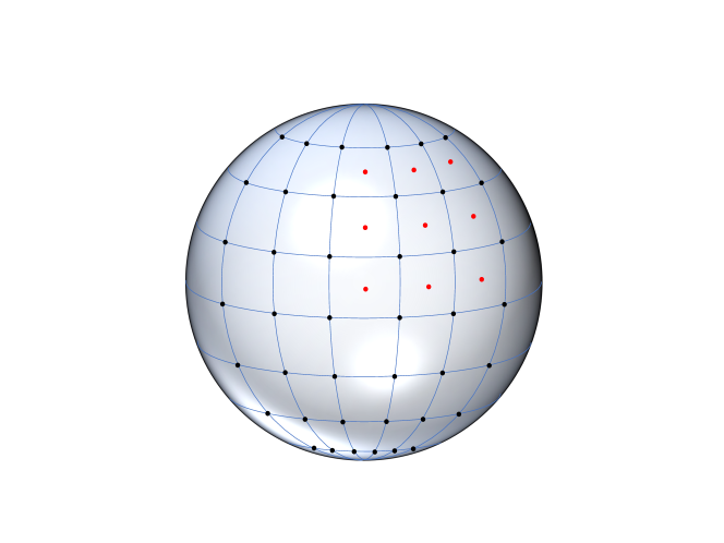
(b) Illustration of the grids for training (black) and assimilation (red, partially plotted) to study the flexibility of LAINR

Figure 12: Grids for training and assimilation

Table 10: Comparison of RMSEs for different filters for LAINR (ours) on the shallow-water dataset with the distinct grid $G^{\prime}$. The relative increments compared to the performances on $G$ are appended in parentheses.

$\sigma^{m}$	$\sigma_{z}^{b}$	EnKF	SEnKF	DEnKF	ETKF	ETKF-Q
0.01	$0.1\sigma_{x}^{b}$	0.09348($+6.9$%)	0.08626($+0.5$%)	0.09318($+8.8$%)	0.09211($+2.2$%)	0.05433($-2.3$%)
0.003	$0.1\sigma_{x}^{b}$	0.06338($-1.2$%)	0.07442($-4.6$%)	0.06308($+5.2$%)	0.06456($-0.3$%)	0.05264($-2.4$%)
0.001	$0.1\sigma_{x}^{b}$	0.05958($+7.2$%)	0.07541($-5.7$%)	0.05758($+6.5$%)	0.05606($-1.5$%)	0.05204($-2.5$%)
0.0003	$0.1\sigma_{x}^{b}$	0.05700($-1.4$%)	0.07678($-10.3$%)	0.05626($+7.6$%)	0.05492($+0.8$%)	0.05202($-3.2$%)
0.0001	$0.1\sigma_{x}^{b}$	0.05761($+0.0$%)	0.07702($-12.6$%)	0.05456($-6.5$%)	0.05723($+4.3$%)	0.05212($-5.3$%)
0.01	$0.01\sigma_{x}^{b}$	0.09448($+8.0$%)	0.08578($+0.0$%)	0.09193($+7.4$%)	0.09170($+1.7$%)	0.05350($-18.1$%)
0.003	$0.01\sigma_{x}^{b}$	0.06254($-2.5$%)	0.07495($-4.0$%)	0.06195($+3.3$%)	0.06243($-3.6$%)	0.05182($-17.6$%)
0.001	$0.01\sigma_{x}^{b}$	0.05483($-1.2$%)	0.07645($-4.5$%)	0.05337($-1.2$%)	0.05468($-3.9$%)	0.05116($-4.1$%)
0.0003	$0.01\sigma_{x}^{b}$	0.05412($-6.0$%)	0.07897($-7.8$%)	0.05171($-1.0$%)	0.05245($-3.8$%)	0.05143($-3.3$%)
0.0001	$0.01\sigma_{x}^{b}$	0.05545($-2.5$%)	0.08031($-8.9$%)	0.05636($-2.0$%)	0.05375($-2.0$%)	0.05252($-5.1$%)

5 Conclusion and future work

In this study, we have proposed a latent assimilation framework called Latent Assimilation with Implicit Neural Representations (LAINR), which offers a new integration of machine learning techniques and data assimilation concepts. Besides, our LAINR framework opens up new possibilities for processing and assimilating complex data systems by using the reduce-order technique. In comparison to existing AutoEncoder-based models, experiments have shown that LAINR surpasses the previous models in terms of not just theoretically appliability but also practical performance.

Non-linear embedding

LAINR’s capability for non-linear embedding introduces the possibility that the complex dynamics of physical states is transformed into a much simpler latent dynamics. Also, experiments have shown that by using the SINR architecture, LAINR outperforms previous AutoEncoder-based non-linear embeddings in terms of both prediction accuracy and compatibility of existing data assimilation algorithms.

Continuous mapping

Unlike the AutoEncoder-based baselines that treat the state field as a discrete grid of state features, LAINR considers the state field as a continuous map, and the special perspective provides a more accurate description of physical features, aiding in the learning of latent representations. Besides, the availability of a continuous field help establish complicated observation operators such as the solution of radiative-transfer models in that interpolation is no longer necessary. Additionally, LAINR is able to handle inputs from partially observed or even irregular grids, which becomes more suitable under potential hardware limitations when complete observations are not always guaranteed such as satellite or radar observations, and as a consequence, its utility scope is wider in real-world scenarios compared with AutoEncoder-based architectures.

Estimation of Uncertainties

As a crucial part for the DA algorithms, the uncertainties of both the latent surrogate model and the encoding process for the physical background estimate can be obtained effectively by our LAINR framework. Such features decrease the cost of empirically tuning with expert knowledge and also enable us to have a better understanding of the uncertainties of the trained networks.

Scalability

LAINR exhibits a clear edge in scalability over previous AutoEncoder-based models. Since the architecture of LAINR uses coordinates as inputs, it effortlessly accommodates increasing dimensionality and resolution, unlike classical models that encounter increased computational costs due to their reliance on a grid of features as inputs.

Nonetheless, it is also important to acknowledge that areas where further research and development are needed. One such aspect is the testing of LAINR on real observation datasets. The performance and robustness of our LAINR framework under real-world conditions would provide further validation of its effectiveness. Additionally, more complicated observation operators need to be incorporated into the experiments since the real observations tends to be highly non-linear such as the solution of radiative-transfer models. Moreover, future work should explore the design of more advanced uncertainty estimator as well.

Reproducibility

All the codes for our proposed LAINR framework and the corresponding experiments are available online at Github (https://github.com/zylipku/LAINR) including the data generation for the shallow-water datasets.

Appendix A Mathematical preliminaries

Proposition A.1.

Given $\{x_{k}\}_{k=1}^{K}\subseteq\mathbb{R}^{n}$, the matrix consists of the first $m$ ($m<n$) left singular vectors of the matrix $X=(x_{1},\cdots,x_{K})\in\mathbb{R}^{n\times K}$ solves the following minimization problem:

$$\min_{A}\sum_{k=1}^{K}\left\|x_{k}-A^{\mathsf{T}}Ax_{k}\right\|^{2}=\min_{A}\left\|(I-A^{\mathsf{T}}A)X\right\|_{F}^{2}\textrm{ subject to }AA^{\mathsf{T}}=I_{m}$$ (67)

for $A\in\mathbb{R}^{m\times n}$, where $\|\cdot\|_{F}$ is the Frobenius norm.

Proof.

For any $A\in\mathbb{R}^{m\times n}$ satisfying $AA^{\mathsf{T}}=I_{m}$ we have

$$\sum_{k=1}^{K}\left\|x_{k}-A^{\mathsf{T}}Ax_{k}\right\|^{2} =\sum_{k=1}^{K}\left\|x_{k}\right\|^{2}-2x_{k}^{\mathsf{T}}A^{\mathsf{T}}Ax_{k}+\left\|A^{\mathsf{T}}Ax_{k}\right\|^{2}$$ (68)

$$=\sum_{k=1}^{K}\left\|x_{k}\right\|^{2}-2x_{k}^{\mathsf{T}}A^{\mathsf{T}}Ax_{k}+x_{k}^{\mathsf{T}}A^{\mathsf{T}}AA^{\mathsf{T}}Ax_{k}$$

$$=\sum_{k=1}^{K}\left\|x_{k}\right\|^{2}-x_{k}^{\mathsf{T}}A^{\mathsf{T}}Ax_{k}=\sum_{k=1}^{K}\left\|x_{k}\right\|^{2}-\|Ax_{k}\|^{2}.$$

Hence the minimization problem is equivalent to the maximization problem

$$\max_{A}\sum_{k=1}^{K}\|Ax_{k}\|^{2}=\max_{A}\|AX\|_{F}^{2}\textrm{ subject to }AA^{\mathsf{T}}=I_{m}.$$ (69)

Take the singular-value decomposition (SVD) for the matrix $X$ as $X=U\Sigma V^{\mathsf{T}}$, where $U\in\mathbb{R}^{n\times n}$ and $V\in\mathbb{R}^{K\times K}$ are orthogonal matrices and $\Sigma=\operatorname*{diag}(\sigma_{1},\cdots,\sigma_{s})$ with $s=\min(n,K)$ and $\sigma_{1}\geq\cdots\geq\sigma_{s}\geq 0$. It follows that

$$\|AX\|_{F}^{2}=\operatorname*{Tr}\left(AX(AX)^{\mathsf{T}}\right)=\operatorname*{Tr}\left(AU\Sigma V^{\mathsf{T}}V\Sigma^{\mathsf{T}}UA^{\mathsf{T}}\right)=\operatorname*{Tr}\left(AU\Sigma\Sigma^{\mathsf{T}}UA^{\mathsf{T}}\right)=\sum_{l=1}^{s}\sigma_{l}^{2}\|Au_{l}\|^{2},$$ (70)

where $u_{l}$ is the $l$-th column of $U$, which is also the left singular vector corresponding to the singular value $\sigma_{l}$. Note that

$$\sum_{l=1}^{s}\|Au_{l}\|^{2}\leq\|AU\|_{F}^{2}=\operatorname*{Tr}\left(AUU^{\mathsf{T}}A^{\mathsf{T}}\right)=\operatorname*{Tr}\left(AA^{\mathsf{T}}\right)=\|A\|_{F}^{2}=m.$$ (71)

Meanwhile, let $B\in\mathbb{R}^{(n-m)\times n}$ such that $(A^{\mathsf{T}},B^{\mathsf{T}})$ is orthogonal, then for each $l$,

$$\|Au_{l}\|^{2}=u_{l}^{\mathsf{T}}A^{\mathsf{T}}Au_{l}=u_{l}\left(I_{n}-B^{\mathsf{T}}B\right)u_{l}=\|u_{l}\|^{2}-\|Bu_{l}\|^{2}\leq\|u_{l}\|^{2}=1.$$ (72)

Therefore,

$$\sum_{l=1}^{s}\sigma_{l}\|Au_{l}\|^{2} =\sum_{l=1}^{m}\sigma_{l}^{2}+\sum_{l=1}^{m}\sigma_{l}^{2}\left(\|Au_{l}\|^{2}-1\right)+\sum_{l=m+1}^{s}\sigma_{l}^{2}\|Au_{l}\|^{2}$$ (73)

$$\leq\sum_{l=1}^{m}\sigma_{l}^{2}+\sigma_{m}^{2}\sum_{l=1}^{m}\left(\|Au_{l}\|^{2}-1\right)+\sigma_{m}^{2}\sum_{l=m+1}^{s}\|Au_{l}\|^{2}$$

$$=\sum_{l=1}^{m}\sigma_{l}^{2}+\sigma_{m}^{2}\left(\sum_{l=1}^{s}\|Au_{l}\|^{2}-m\right)\leq\sum_{l=1}^{m}\sigma_{l}^{2}.$$

Additionally, it is clear that all the equalities hold if $A=(u_{1},\cdots,u_{m})^{\mathsf{T}}$. ∎

Appendix B Detailed configurations for the experiments

B.1 Shallow-water equations

The spherical shallow-water equation on the 2D sphere writes

$$\frac{\mathrm{d}\bm{u}}{\mathrm{d}t} =-f\bm{k}\times\bm{u}-g\nabla h+\nu\Delta\bm{u},$$ (74)

$$\frac{\mathrm{d}h}{\mathrm{d}t} =-h\nabla\cdot\bm{u}+\nu\Delta h,$$

where $\bm{u}=(u,v)^{\mathsf{T}}$ is the 2D velocity field tangent to the sphere surface, and $h$ is the thickness of the fluid layer, both of which are defined on a channel domain $(\lambda,\phi)\in[0,2\pi]\times[-\pi/2,\pi/2]$. The Coriolis parameter $f=2\Omega\sin\phi$ with the angular velocity $\Omega$ and the gravity $g$ are fixed in consistency with the real earth surface. The initial conditions for $\bm{u}$ are given by

$$v|_{t=0}=0,\quad u|_{t=0}=\begin{cases}\frac{u_{m}}{e_{n}}\exp\left(\frac{1}{(\phi-\phi_{0})(\phi-\phi_{1})}\right),&\phi_{0}<|\phi|<\phi_{1},\\ 0&\textrm{otherwise},\end{cases}$$ (75)

which is slightly modified from [31] to create symmetric fields, where $\phi_{0}=\pi/7$ and $\phi_{1}=\pi/2-\phi_{0}$ gives the boundary of the jet. $e_{n}=\exp(-4/(\phi_{1}-\phi_{0})^{2})$ is the normalizer so that the maximal zonal wind $u_{m}$ lies at the jet’s mid-point. The thickness $h$ is initialized as a balanced height field, which is obtained by integrating the balance equation

$$gh(\phi)=gh_{0}-\int^{\phi}au(\phi^{\prime})\left(f+a^{-1}u(\phi^{\prime})\tan\phi^{\prime}\right)\mathrm{d}\phi^{\prime}.$$

The constant $h_{0}$ is chosen so that the global mean of $h$ is $10^{4}$. The balanced field is then perturbed by adding a localized bump

$$h^{\prime}(\lambda,\phi)=\hat{h}\exp\left[-(\lambda/\alpha)^{2}-((\phi_{2}-\phi)/\beta)^{2}\right]\cos\phi,$$ (76)

where $\hat{h}=120$, $\alpha=1/3$, $\beta=1/15$, and $\phi_{2}=\pi/4$.

The datasets for both training and testing are generated via a sample script from the Dedalus project [13] based on Python language within a spectral framework. The maximum velocity $u_{m}$ is randomly sampled from the uniform distribution on the interval $(60,80)$ to generate distinct 20 trajectories for separation of training and testing. Each trajectory has been recorded from 360-th hour to 600-th hour with 1-hour interval to capture rich physical features, and the spatial resolution is set as $128\times 64$. The vorticity $w=\nabla\times\bm{u}$ and the thickness $h$ are the two features for network training and assimilation.

Appendix C Autoencoder baselines

C.1 Detailed network structures

The detailed propagations for both the CAE and AEflow structures are listed in Table 11 and Table 12, respectively, where the batch size is replaced by “$-1$”. As for the activation functions, each convolutional layer is followed by a LeakyReLU [51] with slope 0.2 except the last output layers for the two structures.

Table 11: Forward Propagation in a Convolutional Autoencoder

	Layer	Output Shape
Encoder	Input	$(-1,2,128,64)$
	ConvBlock-1	$(-1,C,64,32)$
	ConvBlock-2	$(-1,C,32,16)$
	ConvBlock-3	$(-1,8,16,8)$
Decoder	Input	$(-1,8,16,8)$
	ConvTransposeBlock-1	$(-1,C,32,16)$
	ConvTransposeBlock-2	$(-1,C,64,32)$
	ConvTransposeBlock-3	$(-1,2,128,64)$

Table 12: Forward Propagation in a AEflow encoder

	Layer	Output Shape
Encoder	Input	$(-1,2,128,64)$
	Conv2d-1	$(-1,4,128,64)$
	ResBlock-1	$(-1,4,128,64)$
	$\cdots\cdots$	$(-1,4,128,64)$
	ResBlock-$N_{\textrm{res}}$	$(-1,4,128,64)$
	Conv2d-2	$(-1,4,128,64)$
	Skip connection from ResBlock-1	$(-1,4,128,64)$
	ConvBlock-1	$(-1,8,64,32)$
	ConvBlock-2	$(-1,16,32,16)$
	ConvBlock-3	$(-1,16,16,8)$
	Conv2d-3	$(-1,8,16,8)$
Decoder	Input	$(-1,8,16,8)$
	Conv2d-1	$(-1,16,16,8)$
	ConvTransposeBlock-1	$(-1,16,32,16)$
	ConvTransposeBlock-2	$(-1,8,64,32)$
	ConvTransposeBlock-3	$(-1,4,128,64)$
	ResBlock-1	$(-1,4,128,64)$
	$\cdots\cdots$	$(-1,4,128,64)$
	ResBlock-$N_{\textrm{res}}$	$(-1,4,128,64)$
	Conv2d-2	$(-1,4,128,64)$
	Skip connection from ResBlock-1	$(-1,4,128,64)$
	Conv2d-3	$(-1,2,128,64)$

C.2 Grid search

As mentioned in Section 4.2, we have conducted a grid search on the configurations for the network structures and then fix the optimal parameters to make a fair comparison with our proposed framework. The grid search results for the CAE and AEflow structures based on the shallow-water dataset are summarized in Table 13. We fix the learning rate as $10^{-3}$ and train all the networks with 10000 epochs to avoid underfitting. The optimal configurations are highlighted in boldface.

Table 13: Training / Testing errors for different configurations of baselines (lower is better)

AutoEncoder		$K=3$	$K=5$	$K=7$
CAE	$C=8$	0.1773	0.1458	0.1761
	$C=16$	0.1598	0.1473	0.1352
	$C=32$	0.1359	0.1108	0.1442
AEflow	$N_{\textrm{res}}=4$	0.1290	0.1062	0.1414
	$N_{\textrm{res}}=8$	0.1235	0.1186	0.7981
	$N_{\textrm{res}}=12$	0.1273	0.1214	0.1341

Appendix D Algorithms for associated Kalman filter methods

D.1 EnKF

The basic Ensenble Kalman Filter (EnKF)

D.1.1 Forecast step

The perturbed forward propagation writes

$$x_{k}^{b,j}=\mathcal{M}_{k}\left(x_{k-1}^{a,j}\right)+\varepsilon_{k}^{M,j},\quad\varepsilon_{k}^{M,j}\sim\mathcal{N}\left(0,\Sigma_{k}^{M}\right).$$ (77)

D.1.2 Analysis step

• Obtain the ensemble mean and anomaly matrix from the ensembles:

  $$x_{k}^{b} =\frac{1}{N}\sum_{j=1}^{N}x_{k}^{b,j},$$ (78)

  $$X_{k}^{b} =\frac{1}{\sqrt{N-1}}\left(x_{k}^{b,j}-x_{k}^{b}\right)_{j=1}^{N}\in\mathbb{R}^{n\times N},$$

  where the background estimate for the covariance matrix is described as $P_{k}^{b}=X_{k}^{b}X_{k}^{b\mathsf{T}}$.

• Sample and calculate the perturbed observation vectors and the corresponding innovation vectors:

  $$z_{k}^{o,j} =y_{k}^{o}+\varepsilon_{k}^{o,j},\quad\varepsilon_{k}^{o,j}\sim\mathcal{N}\left(0,\Sigma_{k}^{o}\right);$$ (79)

  $$d_{k}^{j} =z_{k}^{o,j}-\mathcal{H}_{k}\left(x_{k}^{b,j}\right).$$

• Evaluate the Kalman gain matrix

  $$K_{k} =P_{k}^{b}H_{k}^{\mathsf{T}}\left(H_{k}P_{k}^{b}H_{k}^{\mathsf{T}}+\Sigma_{k}^{o}\right)^{-1}$$ (80)

  $$=X_{k}^{b}X_{k}^{b\mathsf{T}}H_{k}^{\mathsf{T}}\left(H_{k}X_{k}^{b}X_{k}^{b\mathsf{T}}H_{k}^{\mathsf{T}}+\Sigma_{k}^{o}\right)^{-1}$$

  $$=P_{xy}\left(P_{yy}+\Sigma_{k}^{o}\right)^{-1}.$$

  Here, $P_{xy}$ and $P_{yy}$ are given by

  $$P_{xy}=X_{k}^{b}Y_{k}^{b\mathsf{T}},\quad P_{yy}=Y_{k}^{b}Y_{k}^{b\mathsf{T}},$$ (81)

  where $Y_{k}^{b}$ is the anomaly matrix of $\mathcal{H}_{k}\left(x_{k}^{b,j}\right)$.

• Update the analyzed ensembles:

  $$x_{k}^{a,j}=x_{k}^{b,j}+K_{k}d_{k}^{j}.$$ (82)

D.2 SEnKF

Stochastic EnKF (Algorithm 6.3 in [5])

Same as the previous EnKF, except that the Kalman gain matrix is implemented stochastically as

$$K_{k}=X_{k}^{b}Y_{k}^{p\mathsf{T}}\left(Y_{k}^{p}Y_{k}^{p\mathsf{T}}\right)^{-1},$$ (83)

where $Y_{k}^{p}$ is the anomaly matrix of $y_{k}^{p,j}=\mathcal{H}_{k}\left(x_{k}^{b,j}\right)-\varepsilon_{k}^{o,j}$.

D.3 ETKF

ETKF (Algorithm 6.4 in [5])

D.3.1 Forecast step

• Forward propagation:

  $$x_{k}^{b,j}=\mathcal{M}_{k}\left(x_{k-1}^{a,j}\right)+\varepsilon_{k}^{M,j},\quad\varepsilon_{k}^{M,j}\sim\mathcal{N}\left(0,\Sigma_{k}^{M}\right);$$ (84)

  perturbed propagation

D.3.2 Analysis step

• Obtain the ensemble means $x_{k}^{b}$ and the anomaly matrix $X_{k}^{b}$ from the state ensembles $x_{k}^{b,j}$ and $y_{k}^{b}$ and the anomaly matrix $Y_{k}^{b}$ from $y_{k}^{b,j}=\mathcal{H}\left(x_{k}^{b,j}\right)$, respectively as before.

• Calculate the transforming matrix

  $$T_{k}=\left(I_{N}+Y_{k}^{b\mathsf{T}}\left(\Sigma_{k}^{o}\right)^{-1}Y_{k}^{b}\right)^{-1}=\left(I_{N}+S_{k}^{\mathsf{T}}S_{k}\right)^{-1}$$ (85)

  for $S_{k}=\left(\Sigma_{k}^{o}\right)^{-1/2}Y_{k}^{b}$;

• Update the analyzed ensembles with the innovation vector $d_{k}=y_{k}^{o}-y_{k}^{b}$:

  $$w_{k}^{a} =\left(I_{N}+Y_{k}^{b\mathsf{T}}\left(\Sigma_{k}^{o}\right)^{-1}Y_{k}^{b}\right)^{-1}Y^{b\mathsf{T}}\left(\Sigma_{k}^{o}\right)^{-1}\left(y_{k}^{o}-y_{k}^{b}\right)=T_{k}\left(\Sigma_{k}^{o}\right)^{-1}d_{k}$$ (86)

  $$x_{k}^{a,j} =x_{k}^{a}+\sqrt{N-1}X_{k}^{a}[:,j],$$

  where $U$ is a random orthogonal matrix such that $U1=1$.

D.4 ETKF-Q

The ETKF-Q algorithm borrowed from [62] (a special case of IEnKS-Q [29]).

D.4.1 Initialization

Construct $U\in\mathbb{R}^{N\times(N-1)}$ such that

$$\begin{pmatrix}\frac{1}{\sqrt{N}}1_{N}&U\end{pmatrix}$$ (87)

is orthogonal, and let

$$\mathcal{U}=\begin{pmatrix}\frac{1}{N}1_{N}&\frac{1}{\sqrt{N-1}}U\end{pmatrix},$$ (88)

then

$$\mathcal{U}^{-1}=\begin{pmatrix}1_{N}&\sqrt{N-1}U\end{pmatrix}^{\mathsf{T}},$$ (89)

D.4.2 Forecast step

• Forward propagation:

  $$x_{k}^{f,j}=\mathcal{M}_{k}\left(x_{k-1}^{a,j}\right);$$ (90)

• obtain the mean and deviation for $x_{k}^{f}$

  $$\left(x_{k}^{f},\Delta_{x}^{f}\right)=\left(x_{k}^{f,j}\right)_{j}\mathcal{U}$$ (91)

• eigen decomposition (approximately):

  $$\left(\Delta_{x}^{f}\Delta_{x}^{f\mathsf{T}}+\Sigma_{k}^{M}\right)V_{k}\approx V_{k}\Lambda_{k},$$ (92)

  where $V_{k}\in\mathbb{R}^{n\times(N-1)}$ and $\Lambda_{k}\in\mathbb{R}^{(N-1)\times(N-1)}$ are the eigenvectors and eigenvalues of $\Delta_{x}^{f}\Delta_{x}^{f\mathsf{T}}+\Sigma_{k}^{M}$;

• update the deviation:

  $$\Delta_{x}^{b}=V_{k}\Lambda_{k}^{1/2}$$ (93)

• update the ensembles:

  $$\left(x_{k}^{b,j}\right)_{j}=\left(x_{k}^{f},\Delta_{x}^{b}\right)\mathcal{U}^{-1}$$ (94)

D.4.3 Analysis step

• Obtain the ensemble mean and deviation matrix from the ensembles:

  $$\left(x_{k}^{b},\Delta_{x}^{b}\right)=\left(x_{k}^{b,j}\right)_{j}\mathcal{U}$$ (95)

• obtain the mean and deviation for background estimates of observations:

  $$y_{k}^{b,j} =\mathcal{H}_{k}\left(x_{k}^{b,j}\right)$$ (96)

  $$\left(y_{k}^{b},\Delta_{y}^{b}\right) =\left(y_{k}^{b,j}\right)_{j}\mathcal{U}$$

• Transforming matrix:

  $$T_{k}=\left(I_{N-1}+\Delta_{y}^{b\mathsf{T}}\left(\Sigma_{k}^{o}\right)^{-1}\Delta_{y}^{b}\right)^{-1}=\left(I_{N-1}+S_{k}^{\mathsf{T}}S_{k}\right)^{-1}$$ (97)

  for $S_{k}=\left(\Sigma_{k}^{o}\right)^{-1/2}\Delta_{y}^{b}$;

• normalized innovation vector

  $$\delta_{k}=\left(\Sigma_{k}^{o}\right)^{-1/2}\left(y_{k}^{o}-y_{k}^{b}\right)$$ (98)

• Update the analyzed ensembles: (modified from ETKF)

  $$w_{k}^{a} =\left(I_{N-1}+\Delta_{y}^{b\mathsf{T}}\Sigma_{k}^{o}\Delta_{y}^{b}\right)^{-1}\Delta_{y}^{b\mathsf{T}}\left(\Sigma_{k}^{o}\right)^{-1}\left(y_{k}^{o}-y_{k}^{b}\right)=T_{k}S_{k}^{\mathsf{T}}\delta_{k}$$ (99)

  $$x_{k}^{a} =x_{k}^{b}+\Delta_{x}^{b}w_{k}^{a}=x_{k}^{b}+\Delta_{x}^{b}T_{k}S_{k}^{\mathsf{T}}\delta_{k}$$

  $$\Delta_{x}^{a} =\Delta_{x}^{b}\left(I_{N-1}+\Delta_{y}^{b\mathsf{T}}\left(\Sigma_{k}^{o}\right)^{-1}\Delta_{y}^{b}\right)^{-1/2}$$

  $$x_{k}^{a,j} =\left(x_{k}^{a},\Delta_{x}^{a}\right)\mathcal{U}^{-1}$$

References

- [1] Maddalena Amendola, Rossella Arcucci, Laetitia Mottet, César Quilodrán Casas, Shiwei Fan, Christopher Pain, Paul Linden, and Yi-Ke Guo. Data assimilation in the latent space of a convolutional autoencoder. In Maciej Paszynski, Dieter Kranzlmüller, Valeria V. Krzhizhanovskaya, Jack J. Dongarra, and Peter M.A. Sloot, editors, Computational Science – ICCS 2021, pages 373–386, Cham, 2021. Springer International Publishing.
- [2] Troy Arcomano, Istvan Szunyogh, Jaideep Pathak, Alexander Wikner, Brian R. Hunt, and Edward Ott. A machine learning-based global atmospheric forecast model. Geophysical Research Letters, 47(9):e2020GL087776, 2020.
- [3] Rossella Arcucci, Laetitia Mottet, Christopher Pain, and Yi-Ke Guo. Optimal reduced space for variational data assimilation. Journal of Computational Physics, 379:51–69, 2019.
- [4] G. Artana, A. Cammilleri, J. Carlier, and E. Mémin. Strong and weak constraint variational assimilations for reduced order fluid flow modeling. Journal of Computational Physics, 231(8):3264–3288, 2012.
- [5] Mark Asch, Marc Bocquet, and Maëlle Nodet. Data Assimilation. Society for Industrial and Applied Mathematics, Philadelphia, PA, 2016.
- [6] K. Atkinson and W. Han. Spherical Harmonics and Approximations on the Unit Sphere: An Introduction. Lecture Notes in Mathematics. Springer, 2012.
- [7] Thomas Bachlechner, Bodhisattwa Prasad Majumder, Henry Mao, Gary Cottrell, and Julian McAuley. Rezero is all you need: Fast convergence at large depth. In Uncertainty in Artificial Intelligence, pages 1352–1361. PMLR, 2021.
- [8] Dor Bank, Noam Koenigstein, and Raja Giryes. Autoencoders. Machine Learning for Data Science Handbook: Data Mining and Knowledge Discovery Handbook, pages 353–374, 2023.
- [9] Mojtaba Bemana, Karol Myszkowski, Hans-Peter Seidel, and Tobias Ritschel. X-fields: Implicit neural view-, light- and time-image interpolation. ACM Transactions on Graphics (Proc. SIGGRAPH Asia 2020), 39(6), 2020.
- [10] Samy Bengio, Oriol Vinyals, Navdeep Jaitly, and Noam Shazeer. Scheduled sampling for sequence prediction with recurrent neural networks. In Proceedings of the 28th International Conference on Neural Information Processing Systems - Volume 1, NIPS’15, pages 1171–1179, Cambridge, MA, USA, 2015. MIT Press.
- [11] Kaifeng Bi, Lingxi Xie, Hengheng Zhang, Xin Chen, Xiaotao Gu, and Qi Tian. Pangu-weather: A 3d high-resolution model for fast and accurate global weather forecast. arXiv preprint arXiv:2211.02556, 2022.
- [12] Steven L. Brunton, Joshua L. Proctor, and J. Nathan Kutz. Discovering governing equations from data by sparse identification of nonlinear dynamical systems. Proceedings of the National Academy of Sciences, 113(15):3932–3937, 2016.
- [13] Keaton J. Burns, Geoffrey M. Vasil, Jeffrey S. Oishi, Daniel Lecoanet, and Benjamin P. Brown. Dedalus: A flexible framework for numerical simulations with spectral methods. Phys. Rev. Res., 2:023068, Apr 2020.
- [14] Yanhua Cao, Jiang Zhu, Zhendong Luo, and I.M. Navon. Reduced-order modeling of the upper tropical pacific ocean model using proper orthogonal decomposition. Computers & Mathematics with Applications, 52(8):1373–1386, 2006. Variational Data Assimilation and Optimal Control.
- [15] Kang Chen, Tao Han, Junchao Gong, Lei Bai, Fenghua Ling, Jing-Jia Luo, Xi Chen, Leiming Ma, Tianning Zhang, Rui Su, et al. Fengwu: Pushing the skillful global medium-range weather forecast beyond 10 days lead. arXiv preprint arXiv:2304.02948, 2023.
- [16] Peter Yichen Chen, Jinxu Xiang, Dong Heon Cho, Yue Chang, G A Pershing, Henrique Teles Maia, Maurizio M Chiaramonte, Kevin Thomas Carlberg, and Eitan Grinspun. CROM: Continuous reduced-order modeling of PDEs using implicit neural representations. In The Eleventh International Conference on Learning Representations, 2023.
- [17] Peter Yichen Chen, Jinxu Xiang, Dong Heon Cho, Yue Chang, GA Pershing, Henrique Teles Maia, Maurizio Chiaramonte, Kevin Carlberg, and Eitan Grinspun. Crom: Continuous reduced-order modeling of pdes using implicit neural representations. arXiv preprint arXiv:2206.02607, 2022.
- [18] Ricky T. Q. Chen, Brandon Amos, and Maximilian Nickel. Learning neural event functions for ordinary differential equations. International Conference on Learning Representations, 2021.
- [19] Ricky TQ Chen, Yulia Rubanova, Jesse Bettencourt, and David K Duvenaud. Neural ordinary differential equations. Advances in neural information processing systems, 31, 2018.
- [20] Zhiqin Chen and Hao Zhang. Learning implicit fields for generative shape modeling. In Proceedings of the IEEE/CVF Conference on Computer Vision and Pattern Recognition, pages 5939–5948, 2019.
- [21] Sibo Cheng, Jianhua Chen, Charitos Anastasiou, Panagiota Angeli, Omar K. Matar, Yi-Ke Guo, Christopher C. Pain, and Rossella Arcucci. Generalised latent assimilation in heterogeneous reduced spaces with machine learning surrogate models. J. Sci. Comput., 94(1), jan 2023.
- [22] Junyoung Chung, Çaglar Gülçehre, KyungHyun Cho, and Yoshua Bengio. Empirical evaluation of gated recurrent neural networks on sequence modeling. CoRR, abs/1412.3555, 2014.
- [23] Mariana C.A. Clare, Omar Jamil, and Cyril J. Morcrette. Combining distribution-based neural networks to predict weather forecast probabilities. Quarterly Journal of the Royal Meteorological Society, 147(741):4337–4357, 2021.
- [24] Ronald A DeVore, Ralph Howard, and Charles Micchelli. Optimal nonlinear approximation. Manuscripta mathematica, 63:469–478, 1989.
- [25] Emilien Dupont, Hyunjik Kim, S. M. Ali Eslami, Danilo Jimenez Rezende, and Dan Rosenbaum. From data to functa: Your data point is a function and you can treat it like one. In 39th International Conference on Machine Learning (ICML), 2022.
- [26] Emilien Dupont, Hrushikesh Loya, Milad Alizadeh, Adam Goliński, Yee Whye Teh, and Arnaud Doucet. Coin++: Data agnostic neural compression. arXiv preprint arXiv:2201.12904, 2022.
- [27] Geir Evensen. Data Assimilation. Springer Berlin, Heidelberg, 2 edition, 2009.
- [28] Rizal Fathony, Anit Kumar Sahu, Devin Willmott, and J Zico Kolter. Multiplicative filter networks. In International Conference on Learning Representations, 2021.
- [29] Anthony Fillion, Marc Bocquet, Serge Gratton, Selime Gürol, and Pavel Sakov. An iterative ensemble kalman smoother in presence of additive model error. SIAM/ASA Journal on Uncertainty Quantification, 8(1):198–228, 2020.
- [30] Stefania Fresca, Luca Dede’, and Andrea Manzoni. A comprehensive deep learning-based approach to reduced order modeling of nonlinear time-dependent parametrized pdes. Journal of Scientific Computing, 87:1–36, 2021.
- [31] Joseph Galewsky, Richard K. Scott, and Lorenzo M. Polvani. An initial-value problem for testing numerical models of the global shallow-water equations. Tellus A: Dynamic Meteorology and Oceanography, Jan 2004.
- [32] Andrew Glaws, Ryan King, and Michael Sprague. Deep learning for in situ data compression of large turbulent flow simulations. Phys. Rev. Fluids, 5:114602, Nov 2020.
- [33] Anthony Gruber, Max Gunzburger, Lili Ju, and Zhu Wang. A comparison of neural network architectures for data-driven reduced-order modeling. Computer Methods in Applied Mechanics and Engineering, 393:114764, 2022.
- [34] Kaiming He, Xiangyu Zhang, Shaoqing Ren, and Jian Sun. Deep residual learning for image recognition. arXiv preprint arXiv:1512.03385, 2015.
- [35] Hans Hersbach, Bill Bell, Paul Berrisford, Shoji Hirahara, András Horányi, Joaquín Muñoz-Sabater, Julien Nicolas, Carole Peubey, Raluca Radu, Dinand Schepers, Adrian Simmons, Cornel Soci, Saleh Abdalla, Xavier Abellan, Gianpaolo Balsamo, Peter Bechtold, Gionata Biavati, Jean Bidlot, Massimo Bonavita, Giovanna De Chiara, Per Dahlgren, Dick Dee, Michail Diamantakis, Rossana Dragani, Johannes Flemming, Richard Forbes, Manuel Fuentes, Alan Geer, Leo Haimberger, Sean Healy, Robin J. Hogan, Elías Hólm, Marta Janisková, Sarah Keeley, Patrick Laloyaux, Philippe Lopez, Cristina Lupu, Gabor Radnoti, Patricia de Rosnay, Iryna Rozum, Freja Vamborg, Sebastien Villaume, and Jean-Noël Thépaut. The era5 global reanalysis. Quarterly Journal of the Royal Meteorological Society, 146(730):1999–2049, 2020.
- [36] Sepp Hochreiter and Jürgen Schmidhuber. Long short-term memory. Neural Comput., 9(8):1735–1780, nov 1997.
- [37] Chiyu ”Max” Jiang, Soheil Esmaeilzadeh, Kamyar Azizzadenesheli, Karthik Kashinath, Mustafa Mustafa, Hamdi A. Tchelepi, Philip Marcus, Prabhat, and Anima Anandkumar. Meshfreeflownet: A physics-constrained deep continuous space-time super-resolution framework. In Proceedings of the International Conference for High Performance Computing, Networking, Storage and Analysis, SC ’20. IEEE Press, 2020.
- [38] Eugenia Kalnay. Atmospheric Modeling, Data Assimilation and Predictability. Cambridge University Press, 2002.
- [39] Diederik P Kingma and Jimmy Ba. Adam: A method for stochastic optimization. arXiv preprint arXiv:1412.6980, 2014.
- [40] Shunji Kotsuki, Yousuke Sato, and Takemasa Miyoshi. Data assimilation for climate research: Model parameter estimation of large-scale condensation scheme. Journal of Geophysical Research: Atmospheres, 125(1):e2019JD031304, 2020. e2019JD031304 2019JD031304.
- [41] William A Lahoz and Philipp Schneider. Data assimilation: making sense of earth observation. Frontiers in Environmental Science, 2:16, 2014.
- [42] Remi Lam, Alvaro Sanchez-Gonzalez, Matthew Willson, Peter Wirnsberger, Meire Fortunato, Alexander Pritzel, Suman Ravuri, Timo Ewalds, Ferran Alet, Zach Eaton-Rosen, et al. Graphcast: Learning skillful medium-range global weather forecasting. arXiv preprint arXiv:2212.12794, 2022.
- [43] Yann LeCun, Yoshua Bengio, and Geoffrey Hinton. Deep learning. nature, 521(7553):436–444, 2015.
- [44] Kookjin Lee and Kevin T. Carlberg. Model reduction of dynamical systems on nonlinear manifolds using deep convolutional autoencoders. Journal of Computational Physics, 404:108973, 2020.
- [45] Zongyi Li, Nikola Kovachki, Kamyar Azizzadenesheli, Burigede Liu, Kaushik Bhattacharya, Andrew Stuart, and Anima Anandkumar. Fourier neural operator for parametric partial differential equations, 2020.
- [46] Zachary C Lipton, John Berkowitz, and Charles Elkan. A critical review of recurrent neural networks for sequence learning. arXiv preprint arXiv:1506.00019, 2015.
- [47] Zichao Long, Yiping Lu, and Bin Dong. Pde-net 2.0: Learning pdes from data with a numeric-symbolic hybrid deep network. Journal of Computational Physics, 399:108925, 2019.
- [48] Lu Lu, Pengzhan Jin, Guofei Pang, Zhongqiang Zhang, and George Em Karniadakis. Learning nonlinear operators via DeepONet based on the universal approximation theorem of operators. Nature Machine Intelligence, 3(3):218–229, 2021.
- [49] Mantas Lukoševičius and Herbert Jaeger. Reservoir computing approaches to recurrent neural network training. Computer Science Review, 3(3):127–149, 2009.
- [50] Yiqi Luo, Kiona Ogle, Colin Tucker, Shenfeng Fei, Chao Gao, Shannon LaDeau, James S. Clark, and David S. Schimel. Ecological forecasting and data assimilation in a data-rich era. Ecological Applications, 21(5):1429–1442, 2011.
- [51] A.L. Maas, A.Y. Hannun, and A.Y. Ng. Rectifier nonlinearities improve neural network acoustic models. In Proceedings of the International Conference on Machine Learning, Atlanta, Georgia, 2013.
- [52] I. Mehta, M. Gharbi, C. Barnes, E. Shechtman, R. Ramamoorthi, and M. Chandraker. Modulated periodic activations for generalizable local functional representations. In 2021 IEEE/CVF International Conference on Computer Vision (ICCV), pages 14194–14203, Los Alamitos, CA, USA, oct 2021. IEEE Computer Society.
- [53] Philip Nadler, Rossella Arcucci, and Yi-Ke Guo. Data assimilation for parameter estimation in economic modelling. In 2019 15th International Conference on Signal-Image Technology & Internet-Based Systems (SITIS), pages 649–656, 2019.
- [54] Shuli Niu, Yiqi Luo, Michael C. Dietze, Trevor F. Keenan, Zheng Shi, Jianwei Li, and F. Stuart Chapin III. The role of data assimilation in predictive ecology. Ecosphere, 5(5):art65, 2014.
- [55] Mario Ohlberger and Stephan Rave. Reduced basis methods: Success, limitations and future challenges. arXiv preprint arXiv:1511.02021, 2015.
- [56] Jeong Joon Park, Peter Florence, Julian Straub, Richard Newcombe, and Steven Lovegrove. Deepsdf: Learning continuous signed distance functions for shape representation. In Proceedings of the IEEE/CVF conference on computer vision and pattern recognition, pages 165–174, 2019.
- [57] Adam Paszke, Sam Gross, Francisco Massa, Adam Lerer, James Bradbury, Gregory Chanan, Trevor Killeen, Zeming Lin, Natalia Gimelshein, Luca Antiga, Alban Desmaison, Andreas Kopf, Edward Yang, Zachary DeVito, Martin Raison, Alykhan Tejani, Sasank Chilamkurthy, Benoit Steiner, Lu Fang, Junjie Bai, and Soumith Chintala. Pytorch: An imperative style, high-performance deep learning library. In Advances in Neural Information Processing Systems 32, pages 8024–8035. Curran Associates, Inc., 2019.
- [58] Jaideep Pathak, Shashank Subramanian, Peter Harrington, Sanjeev Raja, Ashesh Chattopadhyay, Morteza Mardani, Thorsten Kurth, David Hall, Zongyi Li, Kamyar Azizzadenesheli, Pedram Hassanzadeh, Karthik Kashinath, and Animashree Anandkumar. Fourcastnet: A global data-driven high-resolution weather model using adaptive fourier neural operators. arXiv preprint arXiv:2202.11214, 2022.
- [59] Suraj Pawar and Omer San. Equation-free surrogate modeling of geophysical flows at the intersection of machine learning and data assimilation. Journal of Advances in Modeling Earth Systems, 14(11):e2022MS003170, 2022.
- [60] S. G. Penny, T. A. Smith, T.-C. Chen, J. A. Platt, H.-Y. Lin, M. Goodliff, and H. D. I. Abarbanel. Integrating recurrent neural networks with data assimilation for scalable data-driven state estimation. Journal of Advances in Modeling Earth Systems, 14(3):e2021MS002843, 2022.
- [61] Ethan Perez, Florian Strub, Harm de Vries, Vincent Dumoulin, and Aaron C. Courville. Film: Visual reasoning with a general conditioning layer. In AAAI, 2018.
- [62] Mathis Peyron, Anthony Fillion, Selime Gürol, Victor Marchais, Serge Gratton, Pierre Boudier, and Gael Goret. Latent space data assimilation by using deep learning. Quarterly Journal of the Royal Meteorological Society, 147(740):3759–3777, 2021.
- [63] Allan Pinkus. Basic Properties of n-Widths, pages 9–38. Springer Berlin Heidelberg, Berlin, Heidelberg, 1985.
- [64] Maziar Raissi, Paris Perdikaris, and George E Karniadakis. Physics-informed neural networks: A deep learning framework for solving forward and inverse problems involving nonlinear partial differential equations. Journal of Computational Physics, 378:686–707, 2019.
- [65] Stephan Rasp, Peter D. Dueben, Sebastian Scher, Jonathan A. Weyn, Soukayna Mouatadid, and Nils Thuerey. Weatherbench: A benchmark data set for data-driven weather forecasting. Journal of Advances in Modeling Earth Systems, 12(11):e2020MS002203, 2020. e2020MS002203 10.1029/2020MS002203.
- [66] Stephan Rasp and Nils Thuerey. Data-driven medium-range weather prediction with a resnet pretrained on climate simulations: A new model for weatherbench. Journal of Advances in Modeling Earth Systems, 13(2):e2020MS002405, 2021. e2020MS002405 2020MS002405.
- [67] F. Regazzoni, L. Dedè, and A. Quarteroni. Machine learning for fast and reliable solution of time-dependent differential equations. Journal of Computational Physics, 397:108852, 2019.
- [68] Sebastian Scher and Gabriele Messori. Ensemble methods for neural network-based weather forecasts. Journal of Advances in Modeling Earth Systems, 13(2), 2021.
- [69] M. G. Schultz, C. Betancourt, B. Gong, F. Kleinert, M. Langguth, L. H. Leufen, A. Mozaffari, and S. Stadtler. Can deep learning beat numerical weather prediction? Philosophical Transactions of the Royal Society A: Mathematical, Physical and Engineering Sciences, 379(2194):20200097, 2021.
- [70] Justin Sirignano and Konstantinos Spiliopoulos. Dgm: A deep learning algorithm for solving partial differential equations. Journal of Computational Physics, 375:1339–1364, 2018.
- [71] Vincent Sitzmann, Julien N.P. Martel, Alexander W. Bergman, David B. Lindell, and Gordon Wetzstein. Implicit neural representations with periodic activation functions. In arXiv, 2020.
- [72] O. Talagrand. 4D-VAR: four-dimensional variational assimilation. In Advanced Data Assimilation for Geosciences: Lecture Notes of the Les Houches School of Physics: Special Issue, June 2012. Oxford University Press, 10 2014.
- [73] Matthew Tancik, Pratul P. Srinivasan, Ben Mildenhall, Sara Fridovich-Keil, Nithin Raghavan, Utkarsh Singhal, Ravi Ramamoorthi, Jonathan T. Barron, and Ren Ng. Fourier features let networks learn high frequency functions in low dimensional domains. NeurIPS, 2020.
- [74] Andrew Tangborn and Sara Q. Zhang. Wavelet transform adapted to an approximate kalman filter system. Applied Numerical Mathematics, 33(1):307–316, 2000.
- [75] Silviu-Marian Udrescu and Max Tegmark. Ai feynman: A physics-inspired method for symbolic regression. Science Advances, 6(16):eaay2631, 2020.
- [76] E. Weinan and Bing Yu. The deep ritz method: A deep learning-based numerical algorithm for solving variational problems. Communications in Mathematics and Statistics, 6(1):1–12, March 2018.
- [77] Hilary Weller, John Thuburn, and Colin J. Cotter. Computational modes and grid imprinting on five quasi-uniform spherical c grids. Monthly Weather Review, 140(8):2734 – 2755, 2012.
- [78] Jonathan A. Weyn, Dale R. Durran, and Rich Caruana. Improving data-driven global weather prediction using deep convolutional neural networks on a cubed sphere. Journal of Advances in Modeling Earth Systems, 12(9):e2020MS002109, 2020. e2020MS002109 10.1029/2020MS002109.
- [79] Zhanhong Ye, Hongsheng Liu, Zidong Wang, and Bin Dong. Analysis of the decoder width for parametric partial differential equations. arXiv preprint arXiv:2306.14390, 2023.
- [80] Yuan Yin, Matthieu Kirchmeyer, Jean-Yves Franceschi, Alain Rakotomamonjy, and Patrick Gallinari. Continuous pde dynamics forecasting with implicit neural representations. arXiv preprint arXiv:2209.14855, 2022.
- [81] Junhai Zhai, Sufang Zhang, Junfen Chen, and Qiang He. Autoencoder and its various variants. In 2018 IEEE International Conference on Systems, Man, and Cybernetics (SMC), pages 415–419, 2018.