\DeclareDelimFormat

nameyeardelim,


DeCovarT, a multidimensional probalistic model for the deconvolution of heterogeneous transcriptomic samples

Bastien Chassagnol1,2,*, Grégory Nuel2, Etienne Becht1


1 Institut De Recherches Internationales Servier (IRIS), FRANCE
2 LPSM (Laboratoire de Probabilités, Statistiques et Modélisation), Sorbonne Université, 4, place Jussieu, 75252 PARIS, FRANCE

* bastien_chassagnol@laposte.net

Abstract

Although bulk transcriptomic analyses have greatly contributed to a better understanding of complex diseases, their sensibility is hampered by the highly heterogeneous cellular compositions of biological samples. To address this limitation, computational deconvolution methods have been designed to automatically estimate the frequencies of the cellular components that make up tissues, typically using reference samples of physically purified populations. However, they perform badly at differentiating closely related cell populations.

We hypothesised that the integration of the covariance matrices of the reference samples could improve the performance of deconvolution algorithms. We therefore developed a new tool, DeCovarT, that integrates the structure of individual cellular transcriptomic network to reconstruct the bulk profile. Specifically, we inferred the ratios of the mixture components by a standard maximum likelihood estimation (MLE) method, using the Levenberg-Marquardt algorithm to recover the maximum from the parametric convolutional distribution of our model. We then consider a reparametrisation of the log-likelihood to explicitly incorporate the simplex constraint on the ratios. Preliminary numerical simulations suggest that this new algorithm outperforms previously published methods, particularly when individual cellular transcriptomic profiles strongly overlap.

1 Introduction

The analysis of the bulk transcriptome provided new insights on the mechanisms underlying disease development. However, such methods ignore the intrinsic cellular heterogeneity of complex biological samples, by averaging measurements over several distinct cell populations. Failure to account for changes of the cell composition is likely to result in a loss of specificity (genes mistakenly identified as differentially expressed, while they only reflect an increase in the cell population naturally producing them) and sensibility (genes expressed by minor cell populations are amenable being masked by highly variable expression from major cell populations).

Accordingly, a range of computational methods have been developed to estimate cellular fractions, but they perform poorly in discriminating cell types displaying high phenotypic proximity. Indeed, most of them assume that purified cell expression profiles are fixed observations, omitting the variability and intrinsically interconnected structure of the transcriptome. For instance, the gold-standard deconvolution algorithm CIBERSORT [newman_etal15] applies nu-support vector regression ($\nu$-SVR) to recover the minimal subset of the most informative genes in the purified signature matrix. However, this machine learning approach assumes that the transcriptomic expressions are independent.

In contrast to these approaches, we hypothesised that integrating the pairwise covariance of the genes into the reference transcriptome profiles could enhance the performance of transcriptomic deconvolution methods. The generative probabilistic model of our algorithm, DeCovarT (Deconvolution using the Transcriptomic Covariance), implements this integrated approach.

2 Model

First, we introduce the following notations:

  • $(\boldsymbol{y}=(y_{gi})\in\mathbb{R}_{+}^{G\times N}$ is the global bulk transcriptomic expression, measured in $N$ individuals.

  • $\boldsymbol{X}=(x_{gj})\in\mathcal{M}_{\mathbb{R}^{G\times J}}$ the signature matrix of the mean expression of $G$ genes in $J$ purified cell populations.

  • $\boldsymbol{p}=(p_{ji})\in]0,1[^{J\times N}$ the unknown relative proportions of cell populations in $N$ samples

As in most traditional deconvolution models, we assume that the total bulk expression can be reconstructed by summing the individual contributions of each cell population weighted by its frequency, as stated explicitly in the following linear matricial relationship (Equation 1):

$$\boldsymbol{y}=\boldsymbol{X}\times\boldsymbol{p}$$ (1)

In addition, we consider unit simplex constraint on the cellular ratios, $\boldsymbol{p}$ (Equation 2):

$$\begin{cases}\sum_{j=1}^{J}p_{j}=1\\ \forall j\in\widetilde{J}\quad p_{j}\geq 0\end{cases}$$ (2)

2.1 Standard linear deconvolution model

However, in real conditions with technical and environmental variability, strict linearity of the deconvolution does not usually hold. Thus, an additional error term is usually considered, and without further assumption on the distribution of this error term, the usual approach to retrieve the best of parameters is by minimising the squared error term between the mixture expressions predicted by the linear model and the actual observed response. This optimisation task is achieved through the ordinary least squares (OLS) approach (Equation 3),

$$\boldsymbol{\hat{p}}_{i}^{\text{OLS}}\equiv\operatorname*{arg\,min}_{\boldsymbol{p}_{i}}||\hat{\boldsymbol{y}_{i}}-\boldsymbol{y}_{i}||^{2}=\operatorname*{arg\,min}_{\boldsymbol{p}_{i}}||\boldsymbol{X}\boldsymbol{p}_{i}-\boldsymbol{y}_{i}||^{2}=\sum_{g=1}^{G}\left(y_{gi}-\sum_{j=1}^{J}x_{gj}p_{ji}\right)$$ (3)

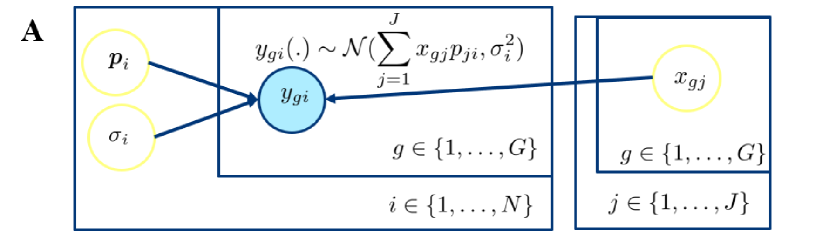
If we additionally assume that the stochastic error term follows a homoscedastic zero-centred Gaussian distribution and that the value of the observed covariates (here, the purified expression profiles) is determined (see the corresponding graphical representation in Figure 1(a) and the set of equations describing it Equation 4),

$$y_{gi}=\sum_{j=1}^{J}x_{gj}p_{ji}+\epsilon_{i},\quad y_{gi}\sim\mathcal{N}\left(\sum_{j=1}^{J}x_{gj}p_{ji},\sigma_{i}^{2}\right),\quad\epsilon_{i}\sim\mathcal{N}(0,\sigma_{i}^{2})$$ (4)

then, the MLE is equal to the OLS, which, in this framework, is given explicitly by Equation 5:

$$\boldsymbol{\hat{p}}_{i}^{\text{OLS}}=(\boldsymbol{X}^{\top}\boldsymbol{X})^{-1}\boldsymbol{X}^{\top}\boldsymbol{y}_{i}$$ (5)

and is known under the the Gauss-Markov theorem.

2.2 Motivation of using a probabilistic convolution framework

In contrast to standard linear regression models, we relax in the DeCovarT modelling framework the exogeneity assumption, by considering the set of covariates $\boldsymbol{X}$ as random variables rather than fixed measures, in a process close to the approach of DSection algorithm and DeMixt algorithms. However, to our knowledge, we are the first to weaken the independence assumption between observations by explicitly considering a multivariate distribution and integrating the intrinsic covariance structure of the transcriptome of each purified cell population.

To do so, we conjecture that the $G$-dimensional vector $\boldsymbol{x}_{j}$ characterising the transcriptomic expression of each cell population follows a multivariate Gaussian distribution, given by Equation 6:

$$\operatorname*{Det}(2\pi\boldsymbol{\Sigma}_{j})^{-\frac{1}{2}}\exp\left(-\frac{1}{2}(\boldsymbol{x}_{j}-\boldsymbol{\mu}_{.j})\boldsymbol{\Sigma}_{j}^{-1}(\boldsymbol{x}_{j}-\boldsymbol{\mu}_{.j})^{\top}\right)$$ (6)

and parametrised by:

  • $\boldsymbol{\mu}_{.j}$, the mean purified transcriptomic expression of cell population $j$

  • $\boldsymbol{\Sigma}_{j}$, the positive-definite (see Definition Section A.1) covariance matrix of each cell population. Precisely, we retrieve it from inferring its inverse, known as the precision matrix, through the gLasso [mazumder_hastie11] algorithm. We define $\boldsymbol{\Theta}_{j}\equiv\boldsymbol{\Sigma}_{j}^{-1}$ the corresponding precision matrix, whose inputs, after normalisation, store the partial correlation between two genes, conditioned on all the others. Notably, pairwise gene interactions whose corresponding off-diagonal terms in the precision matrix are null are considered statistically spurious, and discarded.

To derive the log-likelihood of our model, first we plugged-in the mean and covariance parameters $\zeta_{j}=\left(\boldsymbol{\mu}_{.j},\boldsymbol{\Sigma}_{j}\right)$ estimated for each cell population in the previous step. Then, setting $\boldsymbol{\zeta}=(\boldsymbol{\mu},\boldsymbol{\Sigma}),\quad\boldsymbol{\mu}=(\boldsymbol{\mu}_{.j})_{j\in\widetilde{J}}\in\mathcal{M}_{G\times J},\quad\boldsymbol{\Sigma}\in\mathcal{M}_{G\times G}$ the known parameters and $\boldsymbol{p}$ the unknown cellular ratios, we show that the conditional distribution of the observed bulk mixture, conditioned on the individual purified expression profiles and their ratios in the sample, $\boldsymbol{y}|(\boldsymbol{\zeta},\boldsymbol{p})$, is the convolution of pairwise independent multivariate Gaussian distributions. Using the affine invariance property of Gaussian distributions, we can show that this convolution is also a multivariate Gaussian distribution, given by Equation 7.

$$\boldsymbol{y}|(\boldsymbol{\zeta},\boldsymbol{p})\sim\mathcal{N}_{G}(\boldsymbol{\mu}\boldsymbol{p},\boldsymbol{\Sigma})\text{ with }\boldsymbol{\mu}=(\boldsymbol{\mu}_{.j})_{j\in\widetilde{J}},\quad\boldsymbol{p}=(p_{1},\ldots,p_{J})\text{ and }\boldsymbol{\Sigma}=\sum_{j=1}^{J}p_{j}^{2}\boldsymbol{\Sigma}_{j}$$ (7)

. The DAG associated to this modelling framework is shown in Figure Figure 1(b)).

(a) Standard linear model representation.
Refer to caption
(b) The generative model used for the DeCovarT framework.
Refer to caption
Figure 1: We use the standard graphical convention of graphical models, as depicted in RevBayes webpage. For identifiability reasons, we conjecture that all variability proceeds from the stochastic nature of the covariates.

In the next section, we provide an explicit formula of the log-likelihood of our probabilistic framework, its gradient and hessian, which in turn can be used to retrieve the MLE of our distribution.

2.3 Derivation of the log-likelihood

From Equation 7, the conditional log-likelihood is readily computed and given by Equation 8:

$$\ell_{\boldsymbol{y}|\boldsymbol{\zeta}}(\boldsymbol{p})=C+\log\left(\operatorname*{Det}\left(\sum_{j=1}^{J}p_{j}^{2}\boldsymbol{\Sigma}_{j}\right)^{-1}\right)-\frac{1}{2}(\boldsymbol{y}-\boldsymbol{p}\boldsymbol{\mu})^{\top}\left(\sum_{j=1}^{J}p_{j}^{2}\boldsymbol{\Sigma}_{j}\right)^{-1}(\boldsymbol{y}-\boldsymbol{p}\boldsymbol{\mu})$$ (8)

2.4 First and second-order derivation of the unconstrained DeCovarT log-likelihood function

The stationary points of a function and notably maxima, are given by the roots (the values at which the function crosses the $x$-axis) of its gradient, in our context, the vector: $\nabla\ell:\mathbb{R}^{J}\to\mathbb{R}^{J}$ evaluated at point $\nabla\ell(\boldsymbol{p}):]0,1[^{J}\to\mathbb{R}^{J}$. Since the computation is the same for any cell ratio $p_{j}$, we give an explicit formula for only one of them (Equation 9):

$$\begin{split}\frac{\partial\ell_{\boldsymbol{y}|\boldsymbol{\zeta}}(\boldsymbol{p})}{\partial p_{j}}=&\scriptstyle\frac{\partial\log\left(\operatorname*{Det}(\boldsymbol{\Theta})\right)}{\partial p_{j}}-\frac{1}{2}\left[\frac{\partial(\boldsymbol{y}-\boldsymbol{\mu}\boldsymbol{p})^{\top}}{\partial p_{j}}\boldsymbol{\Theta}(\boldsymbol{y}-\boldsymbol{\mu}\boldsymbol{p})+(\boldsymbol{y}-\boldsymbol{\mu}\boldsymbol{p})^{\top}\frac{\partial\boldsymbol{\Theta}}{\partial p_{j}}(\boldsymbol{y}-\boldsymbol{\mu}\boldsymbol{p})+(\boldsymbol{y}-\boldsymbol{\mu}\boldsymbol{p})^{\top}\boldsymbol{\Theta}\frac{\partial(\boldsymbol{y}-\boldsymbol{\mu}\boldsymbol{p})}{\partial p_{j}}\right]\\ =&\scriptstyle-\operatorname*{Tr}\left(\boldsymbol{\Theta}\frac{\partial\boldsymbol{\Sigma}}{\partial p_{j}}\right)-\frac{1}{2}\left[-\boldsymbol{\mu}_{.j}^{\top}\boldsymbol{\Theta}(\boldsymbol{y}-\boldsymbol{\mu}\boldsymbol{p})-(\boldsymbol{y}-\boldsymbol{\mu}\boldsymbol{p})^{\top}\Theta\frac{\partial\Sigma}{\partial p_{j}}\Theta(\boldsymbol{y}-\boldsymbol{\mu}\boldsymbol{p})-(\boldsymbol{y}-\boldsymbol{\mu}\boldsymbol{p})^{\top}\boldsymbol{\Theta}\boldsymbol{\mu}_{.j}\right]\\ =&{\color[rgb]{0.29296875,0,0.33203125}\definecolor[named]{pgfstrokecolor}{rgb}{0.29296875,0,0.33203125}-2p_{j}\operatorname*{Tr}\left(\boldsymbol{\Theta}\boldsymbol{\Sigma}_{j}\right)}+{\color[rgb]{0,0.4375,0.58203125}\definecolor[named]{pgfstrokecolor}{rgb}{0,0.4375,0.58203125}(\boldsymbol{y}-\boldsymbol{\mu}\boldsymbol{p})^{\top}\boldsymbol{\Theta}\boldsymbol{\mu}_{.j}}\,+{\color[rgb]{0.9921875,0.890625,0.19921875}\definecolor[named]{pgfstrokecolor}{rgb}{0.9921875,0.890625,0.19921875}p_{j}(\boldsymbol{y}-\boldsymbol{\mu}\boldsymbol{p})^{\top}\boldsymbol{\Theta}\Sigma_{j}\boldsymbol{\Theta}(\boldsymbol{y}-\boldsymbol{\mu}\boldsymbol{p})}\end{split}$$ (9)

Since the solution to $\nabla\left(\ell_{\boldsymbol{y}|\boldsymbol{\zeta}}(\boldsymbol{p})\right)=0$ is not closed, we had to approximate the MLE using iterated numerical optimisation methods. Some of them, such as the Levenberg–Marquardt algorithm, require a second-order approximation of the function, which needs the computation of the Hessian matrix. Deriving once more Equation 9 yields the Hessian matrix, $\mathbf{H}\in\mathcal{M}_{J\times J}$ is given by:

$\displaystyle\mathbf{H}_{i,i}$ $\displaystyle=\frac{\partial^{2}\ell}{\partial^{2}p_{i}}={\color[rgb]{0.29296875,0,0.33203125}\definecolor[named]{pgfstrokecolor}{rgb}{0.29296875,0,0.33203125}-2\operatorname*{Tr}\left(\boldsymbol{\Theta}\boldsymbol{\Sigma}_{i}\right)+4p_{i}^{2}\operatorname*{Tr}\left(\left(\boldsymbol{\Theta}\boldsymbol{\Sigma}_{i}\right)^{2}\right)}{\color[rgb]{0,0.4375,0.58203125}\definecolor[named]{pgfstrokecolor}{rgb}{0,0.4375,0.58203125}-2p_{i}(\boldsymbol{y}-\boldsymbol{\mu}\boldsymbol{p})^{\top}\boldsymbol{\Theta}\boldsymbol{\Sigma}_{i}\boldsymbol{\Theta}\boldsymbol{\mu_{.i}}\,-\boldsymbol{\mu}_{.i}^{\top}\boldsymbol{\Theta}\boldsymbol{\mu_{.i}}}\,-$ (10)
$\displaystyle{\color[rgb]{0.9921875,0.890625,0.19921875}\definecolor[named]{pgfstrokecolor}{rgb}{0.9921875,0.890625,0.19921875}2p_{i}(\boldsymbol{y}-\boldsymbol{\mu}\boldsymbol{p})^{\top}\boldsymbol{\Theta}\boldsymbol{\Sigma}_{i}\boldsymbol{\Theta}\boldsymbol{\mu}_{.i}\,-(\boldsymbol{y}-\boldsymbol{\mu}\boldsymbol{p})^{\top}\boldsymbol{\Theta}\left(4p_{i}^{2}\boldsymbol{\Sigma}_{i}\boldsymbol{\Theta}\boldsymbol{\Sigma}_{i}-\boldsymbol{\Sigma}_{i}\right)\boldsymbol{\Theta}(\boldsymbol{y}-\boldsymbol{\mu}\boldsymbol{p})},\quad i\in\widetilde{J}$
$\displaystyle\mathbf{H}_{i,j}$ $\displaystyle=\frac{\partial^{2}\ell}{\partial p_{i}\partial p_{j}}={\color[rgb]{0.29296875,0,0.33203125}\definecolor[named]{pgfstrokecolor}{rgb}{0.29296875,0,0.33203125}4p_{j}p_{i}\operatorname*{Tr}\left(\boldsymbol{\Theta}\boldsymbol{\Sigma}_{j}\boldsymbol{\Theta}\boldsymbol{\Sigma}_{i}\right)}{\color[rgb]{0,0.4375,0.58203125}\definecolor[named]{pgfstrokecolor}{rgb}{0,0.4375,0.58203125}-2p_{i}(\boldsymbol{y}-\boldsymbol{\mu}\boldsymbol{p})^{\top}\boldsymbol{\Theta}\boldsymbol{\Sigma}_{i}\boldsymbol{\Theta}\boldsymbol{\mu_{.j}}-\boldsymbol{\mu}_{.i}^{\top}\boldsymbol{\Theta}\boldsymbol{\mu_{.j}}}\,-$
$\displaystyle{\color[rgb]{0.9921875,0.890625,0.19921875}\definecolor[named]{pgfstrokecolor}{rgb}{0.9921875,0.890625,0.19921875}2p_{j}(\boldsymbol{y}-\boldsymbol{\mu}\boldsymbol{p})^{\top}\boldsymbol{\Theta}\boldsymbol{\Sigma}_{j}\boldsymbol{\Theta}\boldsymbol{\mu}_{.i}\,-4p_{i}p_{j}(\boldsymbol{y}-\boldsymbol{\mu}\boldsymbol{p})^{\top}\boldsymbol{\Theta}\boldsymbol{\Sigma}_{i}\boldsymbol{\Theta}\boldsymbol{\Sigma}_{j}\boldsymbol{\Theta}(\boldsymbol{y}-\boldsymbol{\mu}\boldsymbol{p})},\quad(i,j)\in\widetilde{J}^{2},i\neq j$

in which the coloured sections pair one by one with the corresponding coloured sections of the gradient, given in Equation 9. Matrix calculus can largely ease the derivation of complex algebraic expressions, thus we remind in Appendix (Matrix calculus) relevant matrix properties and derivations 111The numerical consistency of these derivatives was asserted with the numDeriv package, using the more stable Richardson’s extrapolation ([DBLP:journals/toms/Fornberg81])..

However, the explicit formulas for the gradient and the hessian matrix of the log-likelihood function, given in Equation 9 and Equation 10 respectively, do not take into account the simplex constraint assigned to the ratios. While some optimisation methods use heuristic methods to solve this problem, we consider alternatively a reparametrised version of the problem, detailed comprehensively in Appendix Section A.4.

3 Simulations

3.1 Simulation of a convolution of multivariate Gaussian mixtures

To assert numerically the relevance of accounting the correlation between expressed transcripts, we designed a simple toy example with two genes and two cell proportions. Hence, using the simplex constraint (Equation 2), we only have to estimate one free unconstrained parameter, $\theta_{1}$, and then uses the mapping function Equation 13 to recover the ratios.

We simulated the bulk mixture, $\boldsymbol{y}\in\mathcal{M}_{G\times N}$, for a set of artificial samples $N=500$, with the following generative model:

  • We have tested two levels of cellular ratios, one with equi-balanced proportions ($\boldsymbol{p}=(p_{1},p_{2}=1-p_{1})=(\frac{1}{2},\frac{1}{2})$ and one with highly unbalanced cell populations: $\boldsymbol{p}=(0.95,0.05)$.

  • Then, each purified transcriptomic profile is drawn from a multivariate Gaussian distribution. We compared two scenarios, playing on the mean distance of centroids, respectively $\mu_{.1}=(20,22),\mu_{.2}=(22,20)$ and $\mu_{.2}=(20,40),\mu_{.2}=(40,20)$) and building the covariance matrix, $\mathbf{\Sigma}\in\mathcal{M}_{2\times 2}$ by assuming equal individual variances for each gene (the diagonal terms of the covariance matrix, $\operatorname*{Diag}(\boldsymbol{\Sigma_{1}})=\operatorname*{Diag}(\boldsymbol{\Sigma_{1}})=\boldsymbol{I}_{2}$) but varying the pairwise correlation between gene 1 and gene 2, $\operatorname*{\mathbb{C}\text{ov}}\left[{x_{1,2}}\right]$, on the following set of values: $\{-0.8,-0.6,\ldots,0.8\}$ for each of the cell population.

  • As stated in Equation 1, we assume that the bulk mixture, $\mathbf{y}_{.i}$ could be directly reconstructed by summing up the individual cellular contributions weighted by their abundance, without additional noise.

3.2 Iterated optimisation

The extremum, and by extension the MLE, is a root of the gradient of the log-likelihood. However, in our generative framework, the inverse function cancelling the gradient of Equation Equation 8 is non-closed. Instead, iterated numerical optimisation algorithms that consider first or second-order approximations of the function to optimise are used to approximate the roots.

The Levenberg-Marquardt (LM) algorithm bridges the gap between between the steepest descent method (first-order) and the Newton-Raphson method (second-order) by inflating the diagonal terms of the Hessian matrix. Far from the endpoint, a second-order descent is favoured for its faster convergence pace, while the steepest approach is privileged close to the extremum since it allows careful refinement of the step size. Specially, we used the LM implementation of R package marqLevAlg to infer the ratios $\hat{\boldsymbol{p}}$ from the bootstrap simulations, since it includes an additional convergence criteria, the relative distance to the maximum (RDM), that sets apart extrema from spurious saddle points.

3.3 Results

We compared the performance of DeCovarT algorithm with the outcome of a quadratic algorithm that specifically addresses the unit simplex constraint: the negative least squares algorithm (NNLS, [haskell_hanson81]).

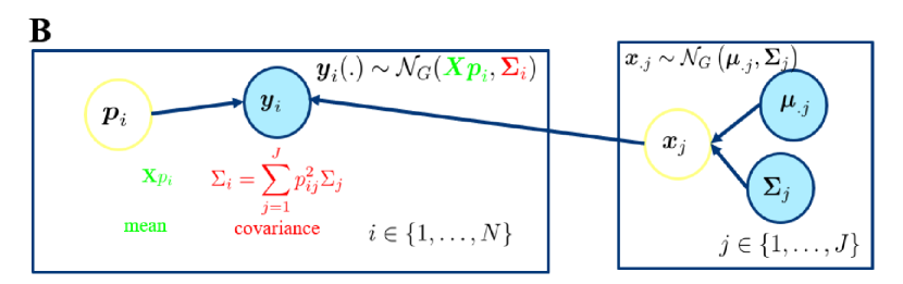
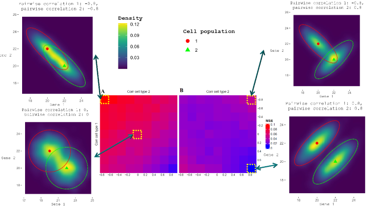
Even with a limited toy example including two cell populations characterised only by two genes, we observe that the overlap was a good proxy of the quality of the estimation: the less the overlap between the two cell distributions, the better the quality of the estimation Figure 2.

Refer to caption
Figure 2: We used the package ComplexHeatmap to display the mean square error (MSE) of the estimated cell ratios, comparing the NNLS output, as implemented in the deconRNASEQ algorithm ([gong_szustakowski13]), in Panel A, with our newly implemented DeCovarT algorithm, in Panel B. The lower the MSE, the least noisy and biased the estimates. In addition, we added the two-dimensional density plot for the intermediate scenario, for which each population is parameterised by a diagonal covariance matrix, and the most extreme scenarios (those with the highest correlation between genes). The ellipsoids represent for each cell population the $95\%$ confidence region and the red spherical icon and the green triangular icon represent respectively the centroids (average expression of gene 1 and gene 2) of cell population 1 and cell population 2.

The package used to generate the simulations and infer ratios from virtual or real biological mixtures with the DeCovarT algorithm is implemented on my personal Github account DeCovarT.

4 Perspectives

The new deconvolution algorithm that we implemented, DeCovarT, is the first one based on a multivariate generative model while complying explicitly the simplex constraint. Hence, it provides a strong basis to further derive statistical tests to assert whether the proportion of a given cell population differs significantly between two distinct biological conditions.

However, we still need to assert its performance in an extended simulation framework. In a numerical setting, we could first increase the dimensionality of our purified datasets by using more realistic parametrisations, using the mean and sparse covariance parameters inferred from purified cellular datasets. Then, we need to evaluate our algorithm in a real-world experience, with both blood and tumoral samples. The Kassandra project would be a good place to start, since the purified database collects a compendium of 9,404 cellular transcriptomic profiles, annotated into 38 blood cellular populations and the performance of Kassandra’s algorithm was benchmarked in $N=517$ samples in 6 public datasets with both flow cytometry annotations and bulk RNA-seq expression, against 8 different standard deconvolution algorithms: 5 reference profile deconvolution algorithms: EPIC [racle_etal17], CIBERSORT [newman_etal15], CIBERSORTx [newman_etal19], quanTIseq [finotello_etal19] and ABIS [monaco_etal19], and 3 marker-based deconvolution algorithms 222Contrary to algorithms based on signature references, marker-based algorithms make the strong asssumption that any discriminant gene, referred to as marker is uniquely expresssed in a cell population.: MCPcounter [becht_etal16] and xCell [aran_etal17].

Finally, the gLasso algorithm used to derive each purified cell accuracy matrix, like any penalty regularisation approach, is subject to parameter shrinkage. Notably, in our setting, shrinkage leads to systematically underestimate the non-zero partial correlations of the precision matrix. A way to circumvent this problem is to only use the support (the non-null inputs) output of the gLasso and use the associated topological constraints within a standard MLE approach to fine-tune the inputs of the precision matrix. One way of doing so would be to infer a directed Gaussian Graphical Model (GGM), however, except in really specific topological configurations, such as chordal graphs, there is no current direct equivalence between the space of undirected Markov graphs, as returned by gLasso, and directed Bayesian graphs ([dahl_etal05]).

Appendix A Optimisation and calculus

A.1 Multivariate distributions and basic algebra properties

Definition A.1: Multivariate Gaussian distributions If random vector $\boldsymbol{X}$ of size $G$ follows a random multivariate Gaussian distribution, $\boldsymbol{X}\sim\mathcal{N}_{G}(\mu,\boldsymbol{\Sigma})$, then its distribution is given by: $$\operatorname*{Det}(2\pi\Sigma)^{-\frac{1}{2}}\exp\left(-\frac{1}{2}(\boldsymbol{x}-\mu)\Sigma^{-1}(\boldsymbol{x}-\mu)^{\top}\right)$$ in which: $\mu=\boldsymbol{X}$ is the $G$-dimensional mean vector $\boldsymbol{\Sigma}$ is a $G\times G$ positive-definite Section A.1 covariance matrix, whose diagonal terms, $\operatorname*{Diag}(\boldsymbol{\Sigma})=[(\operatorname*{\mathbb{V}\text{ar}}\left[{X_{i,j}}\right]),\,\forall(i,j)\in\widetilde{G}^{2},i=j]^{\top}$ are the individual variances of each purified gene transcript in population $j$ and off-diagonal terms, $\boldsymbol{\Sigma}_{i,j}=\operatorname*{\mathbb{C}\text{ov}}\left[{X_{i},X_{j}}\right],\,\forall(i,j)\in\widetilde{G}^{2},i\neq j$ are the covariance between variables. We note $\Theta=\Sigma^{-1}$, the inverse of the covariance matrix, called the precision matrix.
Property A.1: Affine invariance property of multivariate GMMs The two following properties hold for a multivariate Gaussian distribution: if $\boldsymbol{X}\sim\mathcal{N}_{G}(\mu,\boldsymbol{\Sigma})$, then $p\boldsymbol{X}$, with $p$ a constant, follows itself a multivariate Gaussian distribution, given by: $p\boldsymbol{X}\sim\mathcal{N}_{G}(p\mu,p^{2}\Sigma)$ given two independent random vectors $\boldsymbol{X_{1}}\sim\mathcal{N}_{G}(\mu_{1},\boldsymbol{\Sigma_{1}})$ and $\boldsymbol{X_{2}}\sim\mathcal{N}_{G}(\mu_{2},\boldsymbol{\Sigma_{2}})$ following a multivariate Gaussian distribution, then the random variable $\boldsymbol{X_{1}}+\boldsymbol{X_{2}}$ follows itself the multivariate Gaussian distribution: $$X+Y\sim\mathcal{N}_{G}(\mu_{1}+\mu_{2},\boldsymbol{\Sigma_{1}}+\boldsymbol{\Sigma_{2}})$$ By induction, this property generalises to the sum of $J$ independent random vectors of same dimension $\mathbb{R}^{G}$.

Deriving the characteristic function of the multivariate GMM yields directly results reported in Section A.1.

Definition A.2: Definite matrix A symmetric real matrix $\boldsymbol{A}$ of rank $G$ is positive-definite if: $$\boldsymbol{x}^{\top}\boldsymbol{A}\boldsymbol{x}>0,\quad\boldsymbol{x}\in\mathbb{R}^{G}$$ (11) To gain a clearer grasp of the positive-definite constraint imposed on the covariance parameter of a multivariate Gaussian distribution, let’s delve into the most straightforward scenario, in which we assume that any of the individual features exhibit pairwise independence. This particular setup is parametrised by a covariance matrix containing exclusively diagonal elements. If the matrix is not strictly positive-definite, then some of the diagonal elements can display negative values, otherwise that the individual variances for some of the covariates are negative. It is not physically possible and leads to improper, degenerate probability distributions.

A.2 Matrix and linear algebra

Property A.2: Determinant and trace For a squared matrix $A$ of rank $G$ with defined inverse variance $A^{-1}$ and a constant $p$, the following properties hold:
(a) $\operatorname*{Det}(p\boldsymbol{A})=p^{G}\operatorname*{Det}(\boldsymbol{A})$ (b) $\operatorname*{Tr}\left(p\boldsymbol{A}\right)=p\operatorname*{Tr}(\boldsymbol{A})$ (c) $\operatorname*{Det}(A^{-1})=\frac{1}{\operatorname*{Det}(A)}$
The trace operator is additionally invariant under cyclic permutation, illustrated in Section A.2 for three matrices with matching dimensions: $$\operatorname*{Tr}(\boldsymbol{A}\boldsymbol{B}\boldsymbol{C})=\operatorname*{Tr}(\boldsymbol{C}\boldsymbol{A}\boldsymbol{B})=\operatorname*{Tr}(\boldsymbol{B}\boldsymbol{C}\boldsymbol{A})$$
Property A.3: Transpose Given two matrices $\boldsymbol{A}$ and $\boldsymbol{B}$, the following properties hold when computing their transpose:
(a) $(\boldsymbol{A}^{\top})^{\top}=\boldsymbol{A}$ (b) $(\boldsymbol{A}\boldsymbol{B})^{\top}=\boldsymbol{B}^{\top}\boldsymbol{A}^{\top}$ (c) $\left(\boldsymbol{A}^{-1}\right)^{\top}=\boldsymbol{A}^{-1}$22footnotetext: with $\boldsymbol{A}$ a symmetric matrix.
Given two vectors $\boldsymbol{x}$ and $\boldsymbol{y}$ in $\mathbb{R}^{G}$ and $\boldsymbol{A}$ a symmetric matrix of rank $G$, using the properties described above, we have Equation 12 $$\boldsymbol{x}^{\top}\boldsymbol{A}\boldsymbol{y}=\boldsymbol{y}^{\top}\boldsymbol{A}\boldsymbol{x}$$ (12)

A.3 Matrix calculus

Fundamental algebra calculus formulas used to derive first-order (Equation 9) and second-order (Equation 10) derivates are reported in Section A.3 and Section A.3, respectively.

Property A.4: First-order matrix calculus Given two invertible matrices, $A=\boldsymbol{A}(p)$ and $B=\boldsymbol{B}(p)$, functions of a scalar variable $p$, the following matrix calculus hold:
(a) $\frac{\partial\operatorname*{Det}(\boldsymbol{A})}{\partial p}=\operatorname*{Det}(\boldsymbol{A})\operatorname*{Tr}\left(\boldsymbol{A}^{-1}\frac{\partial\boldsymbol{A}}{\partial p}\right)$ (b) $\frac{\partial\boldsymbol{U}\boldsymbol{A}\boldsymbol{V}}{\partial p}=\boldsymbol{U}\frac{\partial\boldsymbol{A}}{\partial p}\boldsymbol{V}$ (c) $\frac{\partial\boldsymbol{A}^{-1}}{\partial p}=-\boldsymbol{A}^{-1}\frac{\partial\boldsymbol{A}}{\partial p}\boldsymbol{A}^{-1}$
From a) and fundamental linear algebra properties enumerated in Section A.2, we can readily compute applying the chain rule property on the logarithm: $$\begin{split}\frac{\partial\log\left(\operatorname*{Det}(\boldsymbol{A})\right)}{\partial p}&=\operatorname*{Tr}\left(\boldsymbol{A}^{-1}\frac{\partial\boldsymbol{A}}{\partial p}\right)\\ \frac{\partial\log\left(\operatorname*{Det}(\boldsymbol{A}^{-1})\right)}{\partial p}&=-\operatorname*{Tr}\left(\boldsymbol{A}^{-1}\frac{\partial\boldsymbol{A}}{\partial p}\right)\end{split}$$ Finally, injecting these first-order matrix derivatives with Section A.2 we have: $$\begin{split}\frac{\partial(\boldsymbol{y}-\boldsymbol{x}p)^{\top}\Theta(\boldsymbol{y}-\boldsymbol{x}p)}{\partial p}&=-2(\boldsymbol{y}-\boldsymbol{x}p)^{\top}\Theta\boldsymbol{x}\\ &=-2\boldsymbol{x}^{\top}\Theta(\boldsymbol{y}-\boldsymbol{x}p)\\ \text{ with }\boldsymbol{A}=\boldsymbol{D}=-\boldsymbol{x}\in\mathbb{R}^{G},\quad\boldsymbol{b}=&\boldsymbol{e}=\boldsymbol{y},\quad\boldsymbol{C}=\boldsymbol{\Theta}\text{ symmetric}\end{split}$$
Property A.5: Second-order matrix calculus Given an invertible matrix $\boldsymbol{A}$ depending on a variable $p$, the following calculus formulas hold: (a) $\frac{\partial^{2}\boldsymbol{A}^{-1}}{\partial p_{i}\partial p_{j}}=\boldsymbol{A}^{-1}\left(\frac{\partial\boldsymbol{A}}{\partial p_{i}}\boldsymbol{A}^{-1}\frac{\partial\boldsymbol{A}}{\partial p_{j}}-\frac{\partial^{2}\boldsymbol{A}}{\partial p_{i}\partial p_{j}}+\frac{\partial\boldsymbol{A}}{\partial p_{j}}\boldsymbol{A}^{-1}\frac{\partial\boldsymbol{A}}{\partial p_{i}}\right)\boldsymbol{A}^{-1}\quad$ (b) $\quad\frac{\partial\operatorname*{Tr}\left(\boldsymbol{A}\right)}{\partial p_{i}}=\operatorname*{Tr}\left(\frac{\partial\boldsymbol{A}}{\partial p_{i}}\right)$ Combining Section A.3 with the linear property of the trace operator yields: $$\frac{\partial^{2}\log\left(\operatorname*{Det}(\boldsymbol{A}^{-1})\right)}{\partial^{2}p}=-\operatorname*{Tr}\left[\boldsymbol{A}^{-1}\frac{\partial^{2}\boldsymbol{A}}{\partial^{2}p_{i}}\right]+\operatorname*{Tr}\left[\left(\boldsymbol{A}^{-1}\frac{\partial\boldsymbol{A}}{\partial p_{i}}\right)^{2}\right]$$

A.4 First and second-order derivation of the constrained DeCovarT log-likelihood function

To reparametrise the log-likelihood function (Equation 8) in order to explicitly handling the unit simplex constraint (Equation 2), we consider the following mapping function: $\boldsymbol{\psi}:\boldsymbol{\theta}\to\boldsymbol{p}\,|\quad\boldsymbol{\theta}\in\mathbb{R}^{J-1},\,\boldsymbol{p}\in]0,1[^{J}$ (Equation 13):

  1. 1.
    $$\boldsymbol{p}=\boldsymbol{\psi}(\boldsymbol{\theta})=\begin{cases}p_{j}=\frac{e^{\theta_{j}}}{\sum_{k<J}e^{\theta_{k}}\,+\,1},\,j<J\\ p_{J}=\frac{1}{\sum_{k<J}e^{\theta_{j}}+1}\end{cases}$$ (13)
  2. 2.

    $\boldsymbol{\theta}=\boldsymbol{\psi}^{-1}(\boldsymbol{p})=\left(\ln{\left(\frac{p_{j}}{p_{J}}\right)}\right)_{j\in\{1,\ldots,J-1\}}$

that is a $C^{2}$-diffeomorphism, since $\boldsymbol{\psi}$ is a bijection between $\boldsymbol{p}$ and $\boldsymbol{\theta}$ twice differentiable.

Its Jacobian, $\mathbf{J}_{\boldsymbol{\psi}}\in\mathcal{M}_{J\times(J-1)}$ is given by Equation 14:

$$\mathbf{J}_{i,j}=\frac{\partial p_{i}}{\partial\theta_{j}}=\begin{cases}\frac{e^{\theta_{i}}B_{i}}{A^{2}},\quad i=j,\,i<J\\ \frac{-e^{\theta_{j}}e^{\theta_{i}}}{A^{2}},\quad i\neq j,\,i<J\\ \frac{-e^{\theta_{j}}}{A^{2}},\quad i=J\end{cases}$$ (14)

with $i$ indexing vector-valued $\boldsymbol{p}$ and $j$ indexing the first-order order partial derivatives of the mapping function, $A=\sum_{j^{\prime}<J}\,e^{\theta_{j^{\prime}}}\,+\,1$ the sum over exponential (denominator of the mapping function) and $B=A-e^{\theta_{i}}$ the sum over ratios minus the exponential indexed with the currently considered index $i$.

The Hessian of the multi-dimensional mapping function $\boldsymbol{\psi(\theta)}$ exhibits symmetry for each cell ratio component $j$, as anticipated in accordance with Schwarz’s theorem. It is is a third-order tensor of rank $(J-1)(J-1)J$, given by Equation 15:

$\displaystyle\frac{\partial^{2}p_{i}}{\partial k\partial j}$ $\displaystyle=\begin{cases}\frac{e^{\theta_{i}}e^{\theta_{l}}\left(-B_{i}+e^{\theta_{i}}\right)}{A^{3}},\,(i<J)\land\left((i\neq j)\oplus(i\neq k)\right)\quad(a)\\ \frac{2e^{\theta_{i}}e^{\theta_{j}}e^{\theta_{k}}}{A^{3}},\,(i<J)\land(i\neq j\neq k)\quad(b)\\ \frac{e^{\theta_{i}}e^{\theta_{j}}\left(-A+2e^{\theta_{j}}\right)}{A^{3}},\,(i<J)\land(j=k\neq i)\quad(c)\\ \frac{B_{i}e^{\theta_{i}}\left(B_{i}-e^{\theta_{i}}\right)}{A^{3}},\,(i<J)\land(j=k=i)\quad(d)\\ \frac{e^{\theta_{j}}\left(-A+2e^{\theta_{j}}\right)}{A^{3}},\,(i=J)\land(j=k)\quad(e)\\ \frac{2e^{\theta_{j}}e^{\theta_{k}}}{A^{3}},\,(i=J)\land(j\neq k)\quad(f)\end{cases}$ (15)

with $i$ indexing $\boldsymbol{p}$, $j$ and $k$ respectively indexing the first-order and second-order partial derivatives of the mapping function with respect to $\boldsymbol{\theta}$. In line $(a)$, $\oplus$ refers to the Boolean XOR operator, $\land$ to the AND operator and $l=\{j,k\}\setminus i$.

To derive the log-likelihood function in Equation 9, we reparametrise $\boldsymbol{p}$ to $\boldsymbol{\theta}$, using a standard chain rule formula. Considering the original log-likelihood function, Equation 8, and the mapping function, Equation 13, the differential at the first order and at the second order is given by Equation 16 and Equation 17, respectively defined in $\mathbb{R}^{J-1}$ and $\mathcal{M}_{(J-1)\times(J-1)}$:

$$\begin{bmatrix}\frac{\partial\ell_{\boldsymbol{y}|\boldsymbol{\zeta}}}{\partial\theta_{j}}\end{bmatrix}_{j<J}=\sum_{i=1}^{J}\frac{\partial\ell_{\boldsymbol{y}|\boldsymbol{\zeta}}}{\partial p_{i}}\frac{\partial p_{i}}{\partial\theta_{j}}$$ (16)
$$\begin{bmatrix}\frac{\partial\ell_{\boldsymbol{y}|\boldsymbol{\zeta}}^{2}}{\partial\theta_{k}\theta_{j}}\end{bmatrix}_{j<J,\,k<J}=\sum_{i=1}^{J}\sum_{l=1}^{J}\left(\frac{\partial p_{i}}{\partial\theta_{j}}\frac{\partial^{2}\ell_{\boldsymbol{y}|\boldsymbol{\zeta}}}{\partial p_{i}\partial p_{l}}\frac{\partial p_{l}}{\partial\theta_{k}}\right)\,+\,\sum_{i=1}^{J}\left(\frac{\partial\ell_{\boldsymbol{y}|\boldsymbol{\zeta}}}{\partial p_{i}}\frac{\partial^{2}p_{i}}{\partial\theta_{k}\theta_{j}}\right)\quad(d)$$ (17)