Mind the (spectral) gap: How the temporal resolution of wind data affects multi-decadal wind power forecasts

Abstract

To forecast wind power generation in the scale of years to decades, outputs from climate models are often used. However, one major limitation of the data projected by these models is their coarse temporal resolution - usually not finer than three hours and sometimes as coarse as one month. Due to the non-linear relationship between wind speed and wind power, and the long forecast horizon considered, small changes in wind speed can result in big changes in projected wind power generation. Our study indicates that the distribution of observed 10min wind speed data is relatively well preserved using three- or six-hourly instantaneous values. In contrast, daily or monthly values, as well as any averages, including three-hourly averages, are almost never capable of preserving the distribution of the underlying higher resolution data. Assuming that climate models behave in a similar manner to observations, our results indicate that output at three-hourly or six-hourly temporal resolution is high enough for multi-decadal wind power generation forecasting. In contrast, wind speed projections of lower temporal resolution, or averages over any time range, should be handled with care.

1 Introduction

Wind is one of the main sources of renewable power and its utilisation is on the rise in many countries, (e.g. Soares-Ramos et al., 2020). It is therefore of uttermost importance to have reliable wind power forecasts in the range of years to decades (i.e. a turbine’s lifetime) for site assessment and reliable future power supply (Copernicus, 2023). However, the high variability and stochasticity of weather and wind introduces uncertainty that makes multi-decadal planning difficult. Furthermore, computational complexity limits the resolution of forecasts; the temporal and spatial resolution of long-term and multi-decadal forecasts are therefore usually much coarser than that of short-term forecasts (Eyring et al., 2016).

But do the low temporal resolution outputs from e.g. climate models provide wind speeds representative of the true site-specific high resolution wind speed distribution? An indicator that this could be the case is the so called wind power spectral gap (Van der Hoven, 1957). Wind speed variability can be assessed in the frequency domain in terms of power spectra by (Fourier-) decomposing high-resolution wind speed observations. This decomposition reveals an amplitude gap between high and low frequencies where the strong variability in high frequencies (on the order of seconds to minutes) is associated with turbulence, while strong low frequency variability (hours to days) is associated with synoptic weather systems (Van der Hoven, 1957),(Stull, 1988). In the gap between the synoptic weather and turbulence peaks in the frequency spectrum are frequencies with little variability; this was found to be in the range of $10^{-3}Hz(\sim 17min)$ to $10^{-4}Hz(\sim 3h)$ by Van der Hoven (1957). However, other research suggests the gap is smaller (Kang and Won, 2016) or may not exist at all (Larsén et al., 2016). This spectral gap is described in many research papers (Horvath et al., 2012), (Kang and Won, 2015), (Larsén et al., 2016), (Lopez-Villalobos et al., 2021) indicating that observations that fall into the corresponding frequencies do not add much knowledge. Given the inconsistency of the width of this spectral gap, the question remains of what temporal resolution we should aim for in multi-decadal wind power forecasting.

Due to the non-linear relationship between wind speed and wind power, small changes in the wind speed distribution can lead to significant changes in wind power generation. However, if the underlying wind speed characteristics are preserved, lower-resolution data is preferred for multi-decadal forecasting to reduce required storage space and potentially also computational costs.

Additionally, multi-decadal wind speed projections should also account for climate change and interannual climate variability (Pryor et al., 2018). Several studies indicate that climate change will affect average wind speeds (McVicar et al., 2012), (Tobin et al., 2015)) as well as wind speed variability (Pryor and Barthelmie, 2010), (Tobin et al., 2016), (Dunn et al., 2019), (Jeong and Sushama, 2019), (Ringkjøb et al., 2020) which will impact wind power generation. In general, it must be assumed that current wind conditions may not be representative of future wind conditions (Jung and Schindler, 2019); we thus often rely on output from climate models to help inform about future potential wind power. But which data (resolution) do we need for meaningful wind speed and power predictions?

There seems to be agreement among researchers that certain temporal resolutions are too low. It is therefore common to account for additional variability using so-called downscaling techniques (Pryor and Barthelmie, 2010). In the past, different statistical downscaling approaches have been introduced, e.g. (Von Storch, 1999), (Tobin et al., 2015), (Shin et al., 2018), as well as dynamical downscaling using regional climate models such as CORDEX (Giorgi and Gutowski Jr, 2015), used by e.g. Davy et al. (2018) and Yang et al. (2022). The question remains, however: what temporal resolution of wind speed data is high enough?

The output from climate models are often available in various temporal aggregations, where some datasets represent temporal averages and other datasets consist of instantaneous values. In the CMIP6 datasets (Eyring et al., 2016), one of the most widely used set of global circulation models (GCMs), wind projections are available as temporal means and instantaneous values (CMIP6 data request, 2016). Currently, however, little focus has been placed on the choice of data and many studies are performed without explicitly stating whether averages or instantaneous values are being used.

With this study we show that the type of data (instantaneous vs averages) influences the wind speed distributions and thus the estimated wind power generation. We also conduct analysis to determine whether there is a temporal resolution that is high enough, i.e. for which added temporal resolution provides little additional information and accuracy. We give recommendations regarding the choice of data and the temporal resolution that downscaling techniques, and climate model outputs, should aim for. To do this, we conduct empirical data analysis using data from eight different mid-latitude sites across Europe and North America. In Section 2 we describe the data and the methodology used. Our results are presented in Section 3 and we discuss their implications in Section 4. Finally, we conclude in Section 5.

2 Methods

To investigate how aggregating wind speed data affects the wind speed distribution we use both parametric and non-parametric approaches. In the main manuscript we focus on observations of turbine-hub-height winds from four sites, with locations shown in Figure 1. We use these as our primary data as they are hub-height data; however, all four sites have a relatively limited observational period of only a few years (see Table 1). We thus also use 10$m$ wind speeds from an additional four observational met masts from locations across Germany (see Figure A.1 for locations) that have between $18$ to $34$ years of data available. These data show very similar results to the hub-height datasets (analysis presented in the supplementary material in Appendix A). We also use these longer datasets to analyze multi-decadal tendencies of wind power generation in Section 3. In the following we first give a description of the data used and then describe our methodology.

Data

We investigate wind speed observations using open-source high met mast wind data of four mid-latitude locations. All of the wind speeds are either measured at wind turbine hub-height directly, i.e. by nacelle anemometers (sites Penmanshiel and Kelmarsh) or by high met masts (sites NWTC and Owez). The observation heights are between $59m$ and $116m$ and all of the measurements are provided as 10min averages, a very common aggregation-level of wind resource data (Harper et al., 2010). In Table 1 we present static information of the observation sites. Static information of the longer datasets (at 10$m$ height) is presented in Table A.1. Unless specified otherwise, the following abbreviations for the datasets can be found in the top left corner of figures: a) Kelmarsh, b) Penmanshiel, c) NWTC, d) Owez, e) Aachen, f) Zugspitze, g) Boltenhagen, h) Fichtelberg.

To bring the data to a format where we can compare different temporal resolutions, we pre-process the data by excluding all days where at least one observation is missing. We then average the 10 min wind speed observations to three-hourly, six-hourly and daily data: the $n$’th wind speed value $w_{n}$ in the time-series averaged over $t$ consecutive time steps is computed as

$$w^{t}_{n}=\frac{1}{t}\sum_{i=nt}^{nt+t}w^{1}_{i},$$ (1)

where $t=18$ (three-hourly), $36$ (six-hourly) and $144$ (daily) respectively; for $t=1$ we get the original 10 min resolution time series $w^{1}$. In addition to calculating averages, we also consider wind speed time series of lower resolution, which we call instantaneous values. To do so, we use wind speed measurements every $t$’th time step only and exclude all other wind speed measurements $w_{i}$ where $i\neq nt$. The results are eight observations per day (every three hours), four observations per day (every six hours) and one observation per day respectively.

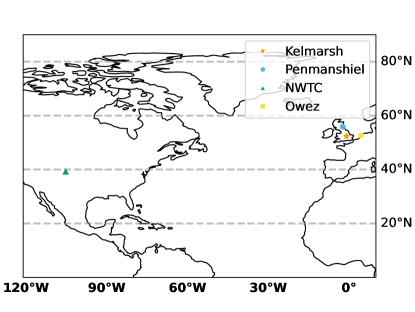
Figure 1: Locations of the two wind farms in the UK and the tall towers in central North America and the Netherlands. Our hub-height observation locations include one mountainous site (NWTC), one off-shore site (Owez), one coastal site (Penmanshiel) and one site on flat terrain (Kelmarsh). Penmanshiel and Kelmarsh are wind farm sites, their wind speeds are therefore influenced by wake effects of the surrounding turbines (e.g. González-Longatt et al., 2012) and we only used one turbine for our evaluations.

Name	Country (Lat, Lon)	Temporal resolution in min	Observation period (Number of days)	Observation height in $m$	Mean wind speed (variance) in $\frac{m}{s}$	Data source
Kelmarsh	United Kingdom (52.40, -0.95)	10	2016-2021 (1687)	78.5	6.25 (7.70)	Plumley (2022a)
Penmanshiel	United Kingdom (55.90, -2.31)	10	2016-2021 (1522)	59	7.27 (15.30)	Plumley (2022b)
Owez	Netherlands (52.61, 4.39)	10	2012-2017 (1148)	116	4.82 (13.02)	Ramon et al. (2020), Ramon et al. (2022a)
NWTC	United States (39.21, -105.23)	10	2005-2010 (1083)	87	8.37 (16.55)	Ramon et al. (2020), Ramon et al. (2022b)

Table 1: Static data of the four different sites with hub-height measurements. Our chosen datasets cover a large range of observation heights as well as different mean wind speeds and variances.

Comparing wind speed distributions

To determine whether wind speed distributions from data of different temporal resolution are statistically different, we compute pairwise Kolmogorov-Smirnov test statistics of cumulative density distributions

$$F_{W}(w)=P(W\leq w).$$ (2)

The Kolmogorov-Smirnov statistic $D$ is given by:

$$D=\sup\limits_{w}|T(w)-S(w)|$$ (3)

where $w$ are the wind speed values, $T$ and $S$ are the wind speed distributions to be compared, and the supremum, $\sup$, is the largest value of the set of values $|T(w)-S(w)|$ across all $w$. The Kolmogorov-Smirnov test only takes the largest absolute difference between the two distributions across all $w$ values into account and we identify a statistically significant difference if the $p$-value of an individual test is $p\leq 0.05$.

Modeling wind speeds using Weibull distributions

The Kolmogorov-Smirnov test can tell us whether wind distributions of different temporal resolution differ; in order to quantify the differences found, we model the wind speeds, $w$, as Weibull distributions. This is done by fitting the parameters of a three-parameter Weibull distribution,

$$f(w;\beta,\lambda,\theta)=\frac{\beta}{\lambda}(\frac{w-\theta}{\lambda})^{\beta-1}e^{-(\frac{w-\theta}{\lambda})^{\beta}}$$ (4)

to the different temporal resolution datasets. The three-parameter Weibull distribution described in Equation 4 is defined by $w\geq\theta$ and $f(w;\beta,\lambda,\theta)=0$ for $w<0$ where $\beta>0$ is the shape parameter, $\lambda>0$ is the scale parameter and $\theta$ is the location parameter of the distribution which equals the lowest possible value of the distribution. For $\beta\approx 3$, the Weibull distribution approximates a Gaussian distribution, while $3>\beta\geq 1$ corresponds to a right-skewed distribution, and $\beta>3$ corresponds to a left-skewed distribution, for $\beta<1$ the density values are steadily decreasing with increasing $w$. $\lambda$ represents the variability, i.e. smaller values of $\lambda$ are associated with less variability (Rinne, 2008). We fit the parameters using Maximum Likelihood Estimation (MLE). This approach requires maximizing the likelihood function

$$L=\prod_{i=1}^{n}f(w_{i};\beta,\lambda,\theta).$$ (5)

We can then evaluate the change of the parameters when wind speeds are averaged or discarded to produce datasets with different temporal resolution. While Weibull distributions are commonly used to model wind speed distributions (e.g. Mert and Karakuş, 2015), we additionally use a generalized Gamma distribution to test the sensitivity of our results to the choice of underlying distribution. The conclusions are unchanged (figures shown in the appendix) and we therefore consider our results to be insensitive to the distribution choice.

Validating the Weibull parametrization

Using a kernel density estimation we confirm that Weibull distributions are a reasonable representation of our data, with the exception of monthly averages. The kernel density estimator $\hat{f}$ of an unknown density $f$ at a point $x$ is defined by

$$\hat{f}_{h}(x)=\frac{1}{nh}\sum_{i=1}^{n}K(\frac{x-x_{i}}{h}),$$ (6)

where we choose $K$ to be the Gaussian kernel

$$K(x,h)=\exp(-\frac{x^{2}}{2h^{2}}).$$ (7)

The band-width $h$ is selected using Scott’s rule (Scott, 2015).

Figures A.2 and A.4 show kernel density estimations for averaged and instantaneous wind speeds respectively; it is clear that monthly values can not be described by a Weibull distribution and thus we do not include this temporal resolution in subsequent analysis. To validate the fit of the Weibull distributions to the original wind speed distributions we generate quantile-quantile plots of the observations of length $\frac{l}{t}$ against $\frac{l}{t}$ randomly drawn samples from the corresponding Weibull distribution; these plots are shown in Figure A.5 and Figure A.6. The Weibull distributions generally provide a good fit to the data, although in some locations the fit is less good at higher wind speeds.

Power generation and transferability of results

As a last step, we relate the insights from the wind speed distributions to multi-decadal wind power forecasts. Wind power generation is often forecasted using hub-height wind speed forecasts with a turbine-specific wind power curve (Wang et al., 2019) that describes the relationship between wind (speed) and potential wind power generation and is highly non-linear. We apply the Enercon E92/2350 wind power curve,visualized in Figure 2. Given the relatively short duration of the main observational datasets we use in this study (around 3-5 years of non-missing data) and our interest in multi-decadal forecasts, we study potential power generation using four $18$ to $34$ year long wind speed datasets.

Additionally, to determine whether the results we find for observational datasets are also applicable to climate model data, we repeat our analysis using data generated by the historical run of the MPI-ESM1-2-LR general circulation model (Eyring et al., 2016) which was the only model with three-hourly data available on the ESGF node (WCRP CMIP6, 2023) at the time of research.

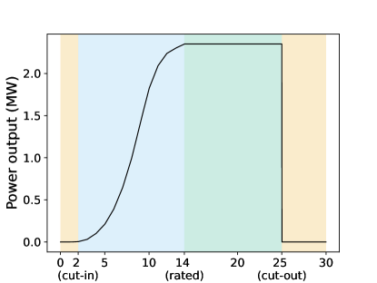
Figure 2: Wind power curve of Enercon E92/2350 turbine. The relationship between wind speed and wind power can be roughly divided into four different regions: No power is generated if the wind speed is below the cut-in wind speed or if the wind speed is above the cut-out wind speed where the turbine is shut down to protect it from damage  . In between, wind power generation first increases rapidly with increasing wind speed  . Once the maximum wind speed that the wind turbine can convert to power is reached, the power output is usually constant until the wind speed exceeds the cut-out wind speed  .

3 Results

We analyze the distributions of wind speed averages and instantaneous wind speed time series, and find consistent results across all sites investigated: averaging introduces shifts to the wind speed distributions, while three-hourly and six-hourly instantaneous data are usually close to the original. This is clearly demonstrated in Figure 3, with differences between 10min wind speeds and averaged data (left hand column) larger than the differences between 10min wind speeds and instantaneous wind speeds of lower resolution (right hand column). Similar patterns can be observed in the four longer datasets, see Figure A.7.

The impact of averaging can also be seen in the variance of the data: while averaging does not affect the mean it reduces the variance of the averaged time series (Figure 4). In contrast, three-hourly and six-hourly instantaneous values (dashed lines in Figure 4) preserve the variance, with daily instantaneous values preserving substantially more of the variance than daily averages, and at some sites, more than six-hourly averages.

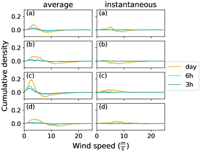
Figure 3: Difference of cumulative densities from the 10min data to the other temporal resolution datasets for average wind speeds (left) and instantaneous wind speeds (right). It can be seen that the averaged wind speeds are visually distinguishable, which is less the case for instantaneous wind speeds, particularly for data with a temporal resolution of six-hourly or higher.

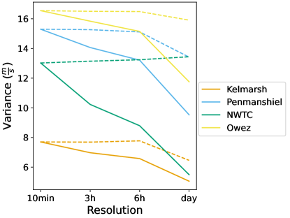
Figure 4: Variances of averaged (solid lines) and instantaneous (dashed lines) values. The variances steadily decrease when wind speeds are averaged and stay close to the 10min variances for the instantaneous three-hourly and six-hourly distributions.

Kolmogorov-Smirnov tests

To quantify whether the difference between the 10min wind speed distribution and the averaged and instantaneous distributions of lower resolution are statistically significant we compute Kolmogorov-Smirnov test statistics of their cumulative density distributions pairwise. The results for the Penmanshiel site are presented in Table 2 (for averaged data) and Table 3 (instantaneous data), where values in bold indicate no statistically significant difference in the distributions, i.e. that using the dataset of lower temporal resolution may retain all information about the wind speed distribution. We observe that all averaged distributions, as well as daily instantaneous distributions, differ significantly from the 10min wind speeds (right-most column), whilst three- and six-hourly instantaneous values are not distinguishable from the 10 min data. The results for all other locations are very similar (see Table A.2 to Table A.15): in general, averages do not preserve the wind speed distribution, and three- and six-hourly instantaneous values are almost always not statistically distinguishable from the 10 min data.

	daily	six-hourly	three-hourly	10min
daily	$\mathbf{1}$	$1.12\cdot 10^{-3}$	$2.94\cdot 10^{-5}$	$1.40\cdot 10^{7}$
six-hourly		$\mathbf{1}$	$\mathbf{4.41\cdot 10^{-1}}$	$5.83\cdot 10^{-3}$
three-hourly			$\mathbf{1}$	$5.83\cdot 10^{-3}$

Table 2: Test statistics of Kolmogorov-Smirnov test for Penmanshiel averages. We reject the hypothesis that the wind speed distributions are equal if $p\leq 5\cdot 10^{-2}$. Therefore, only the three-hourly averages are not significantly different from six-hourly averages.

‘ daily six-hourly three-hourly 10min daily $\mathbf{1}$ $3.03\cdot 10^{-2}$ $2.34\cdot 10^{-2}$ $6.62\cdot 10^{-3}$ six-hourly $\mathbf{1}$ $\mathbf{1.00}$ $\mathbf{9.58\cdot 10^{-1}}$ three-hourly $\mathbf{1}$ $\mathbf{8.07\cdot 10^{-1}}$

Table 3: Test statistics of Kolmogorov-Smirnov test for Penmanshiel instantaneous data. We reject the hypothesis that the wind speed distributions are equal if $p\leq 5\cdot 10^{-2}$ which reveals that only daily instantaneous values are significantly different from all other distributions.

Changes in Weibull parameters

The cumulative density plots and Kolmogorov-Smirnov tests indicate that wind speed distributions are likely to change when wind speeds are averaged and likely to stay similar when measurements are discarded, at least until around six-hourly resolution. The aim of the next steps is to quantify these changes by parameterizing the distributions as Weibull distributions.

Figure 5 shows the values of the three Weibull parameters for the different aggregation levels for averaging (top row) and instantaneous (bottom row). The shape parameter $\beta$ stays approximately constant across all aggregation levels and types, for both averaged and instantaneous data. For averaging, the location parameter $\theta$ increases with higher aggregation levels. This is consistent with the lowest values of the dataset increasing as they are averaged. Conversely, with lower resolution instantaneous data, the lowest values remain similar, leading to similar $\theta$ for all resolutions studied. The scale parameter $\lambda$ decreases with increased averaging length, and remains relatively constant for instantaneous data, consistent with the changes in variance shown in Figure 4. We observe very similar results for $\sim 30$ years of data measured at $10m$ height (see Figure A.8 and Figure A.9). In addition, two of our observational sites, NWTC and Owez, have wind speed data at multiple heights, ranging from $10m$ to $130m$; the changes in Weibull parameters seen in Figure 5 are found at all different heights studied (see Figure A.10).

To test for robustness of our results we also use an MLE to fit a generalized Gamma distribution (see Appendix for details); both Weibull and Gamma distributions are regarded as suitable statistical models for wind speed data (e.g. Mert and Karakuş, 2015). We find very similar results (see Figure A.11 to Figure A.14), with large changes in parameters when averaging data, and relatively small changes for three- and six-hourly instantaneous values. This suggests our conclusions are not sensitive to our choice of parameterization.

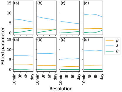
Figure 5: Parameters when data are averaged (top row) or discarded (bottom row) for four different datasets a) Kelmarsh b) Penmanshiel c) NWTC d) Owez. The Weibull parameters change when wind speeds are averaged and stay similar when values are discarded. The corresponding non-parameterized wind speed distributions are visualized in Figure A.2 and Figure A.4.

Implications for multi-decadal wind power forecasting

As introduced in Section 1, wind speeds and wind speed variability are subject to interannual variability and climate change. Hence, for multi-decadal wind power forecasts climate models can provide useful information (e.g. Tobin et al., 2015). To understand how our results apply on multi-decadal timescales, we repeat our analysis using data from four sites where multiple decades of $10m$ wind speed observations are available. We also repeat our analysis on climate model output data to determine whether our conclusions are applicable to model data. We extract $10m$ wind speeds from the historical run of the CMIP6 model MPI-ESM1-2-LR for grid points closest to these four longer-term observational sites (locations shown in Figure A.1). We only use direct output from the model, and thus at daily temporal resolution we do not have instantaneous values, only averages.

For these multi-decadal datasets the Kolmogorov-Smirnov tests and Weibull parameterization analysis produce results comparable to those for the hub-height observations shown in the previous sections. The parameters of fitted Weibull distributions behave similarly in response to changing temporal resolution, with a decrease of $\lambda$ as temporal resolution decreases indicating a decrease in variability (see Figure 6). The climate model data do not show an increase in $\theta$ with decreasing temporal resolution, although for three-hourly and six-hourly averages $\theta$ fitted to the climate model data is very close to the parameters fitted to the observational data.

So far we have only looked at wind speeds and their distributions. However, these are just a proxy for wind power – our variable of interest – and wind power depends non-linearly on wind speed. To estimate the power a wind turbine could generate over its lifetime, we apply the Enercon E92/2350 power curve (see Figure 2) to the four multi-decadal observational wind speed datasets as well as to the wind speeds from the corresponding closest grid-points in the CMIP6 dataset. We then compare the expected cumulative power generation of the highest available resolution (10min in observations and three-hourly instantaneous values in CMIP6 model) to lower resolutions (three-hourly, six-hourly, and daily averages and instantaneous values). Although the highest available resolution in the CMIP6 model is only three-hourly, our previous analysis shows that these values are closely aligned with 10min data.

Figure 7 shows the expected cumulative power generation using wind speed observations of different resolutions. We show this as a fraction of the total power generation achieved when applying the wind power curve to the 10min observational wind speed data and integrating over the whole time period. The dotted gray line shows 100% and thus if the expected cumulative power generation reaches this threshold without overshooting we consider the change introduced by the temporal resolution to be small. The top row of Figure 7 shows that averaging values, particularly to daily, but even to three- or six-hourly at some locations, can lead to relatively large errors in estimated power generation, with errors of up to -34.48% (daily average), -15.45% (six-hourly average), and -10.06% (three-hourly average). Conversely, three-hourly and six-hourly instantaneous values, shown in the bottom row, reveal very similar results to the 10min data, with errors less than 2%.

Figure 8 demonstrates that very similar results are found using the output from the MPI-ESM1-2-LR global climate model, with results given relative to the total amount of power generated using three-hourly instantaneous values. In all cases six-hourly instantaneous values are closest to three-hourly instantaneous values, followed by three-hourly averages and six-hourly averages; daily averages differ substantially.

Reducing temporal resolution leads to an underestimation of expected power generation at all sites studied except for daily instantaneous values at Zugspitze (Figure 7 bottom row, site (f)), a site with relatively high mean wind speeds and high wind speed variance, situated at a high elevation above sea level ($2956m$). This is very likely a function of the particular wind turbine power curve we have chosen. It is important to note that in all cases, both with observational data and climate projections, the difference in power generation compared to higher-resolution data increases with an increasing forecast horizon and does not average out - the shift in the wind distribution leads to a systematic error in wind power estimation. In general, averaging tends to result in an underestimation of expected power generation, while discarding values has only minor impacts.

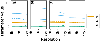
Figure 6: Parameters of Weibull distribution fitted to observational data averages (dashed lines) of the four multiple-decadal sites and to the closest grid points in the CMIP6 MPI-ESM1-2-LR dataset (solid lines). The parameter $\lambda$ decreases in all cases when comparing three-hourly to daily averages, indicating a decrease in variability. The location parameter $\beta$ does not show any consistent trends. $\theta$ increases with daily averages in observational data, but not in the CMIP6 data.

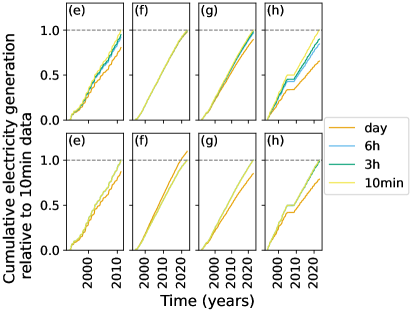
Figure 7: Cumulative power generation of daily, six-hourly and three-hourly values relative to the total 10min wind power generation computed by feeding the wind speeds into a power curve. Top row: Average values underestimate wind power generation – the longer the forecast the higher the error. Bottom row: Instantaneous values every three or six hours only introduce minor errors. Daily data is in no case a good proxy. The power generation gap at the Fichtelberg site between $\sim 2005$ and $2010$ stems from various missing observations. Absolute errors are reported in Table A.16.

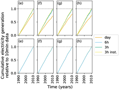
Figure 8: Cumulative power generation of daily, six-hourly and three-hourly values relative to three-hourly instantaneous (3h inst.) wind power generation at the four CMIP6 locations closest to e) Aachen, f) Zugspitze, g) Boltenhagen, h) Fichtelberg computed by feeding the wind speeds into a power curve. Top row: Average values underestimate wind power generation. Bottom row: Instantaneous values (note that daily instantaneous values were not available as direct output, and so are not included). Using six-hourly instantaneous values introduces only minor errors relative to three-hourly instantaneous values.

4 Discussion

Global climate models simulate climate dynamics physically using partial differential equations. Their long forecast horizons make them computationally expensive with large storage space needs and their output is usually provided with a temporal resolution ranging from three hours to one month, either as instantaneous or averaged values. Using hub-height wind speed observations, this study investigates how the temporal resolution of wind speed data affects the wind speed distributions. Using multi-decadal observational datasets at 10$m$ height we study the corresponding potential power generation and which time resolution is actually necessary.

Using hub-height data we find that in all cases investigated, three-hourly and six-hourly instantaneous observations well-preserve the underlying 10min wind speed distribution, whilst three- and six-hourly averaging leads to distributional shifts. However, whether a significant wind speed distribution shift results in a significant change in wind power generation depends on the turbine and its corresponding power curve. Our results, using an example turbine power curve, indicate that the differences in wind distribution highlighted in this study can lead to accumulating errors when power generation is forecasted for years to decades (compare Figure 7 and Figure 8).

Our results are consistent across different observational sites and a GCM. We can therefore give two suggestions when working with wind speed projections for wind power modelling. First, instantaneous wind speed projections should be preferred over wind speed averages, as sub-sampling wind speed data introduces relatively minor errors in contrast to averaging wind speeds, where we observe a characteristic distributional shift. This shift associated with averaging data indicates that we might consistently over- or underestimate wind power generation. Second, instantaneous wind speed projections of six or three hours suffice, whilst daily data may be too low resolution, even with instantaneous values. For our sites temporal downscaling or either three- or six- hourly data is unlikely to provide substantial improvement in accuracy. For example, instantaneous observational wind speeds with a three-hourly temporal resolution lead to errors of less than $0.29\%$, with six-hourly data leading to errors of less than $1.57\%$. The experiments conducted using climate model data support these results. This knowledge can be useful to reduce storage space almost loss-free and decrease computational complexity in further applications using the data.

The primary shortcomings of our investigations include a potential lack of generalizability across turbines, sensitivity to our underlying highest temporal data resolution, and uncertain transferability to other climate models. More specifically, as wind speed data measured at hub-height is often confidential, we are limited to relatively few datasets. Furthermore, for site assessment, wind speeds are usually transformed to hub-height which is non-trivial (e.g. Bañuelos-Ruedas et al., 2010). However, the close agreement of results from stations across a range of different locations, including different local geography (off-shore, on-shore, different altitudes and local topography), suggests that our results likely hold for the majority of locations. For 7 out of the 8 locations studied, using daily instantaneous or average values underestimates the power generation (see Figure 7), while six-hourly values are good approximations. For one station, however, the daily instantaneous data is an overestimate; understanding the conditions under which daily data over- or under-estimates the power generation would be useful for studies in which only daily data is available. In addition, while the Enercon power curve we use in this study has the characteristic shape of any modern horizontal wind turbine power curve, it is not necessarily representative of the turbines at a particular site.

Regarding the sensitivity to the underlying data resolution, we use data in 10min resolution, hence variability on shorter time scales – often associated with turbulence (e.g. Stull, 1988) – is not preserved. However, higher temporal resolution data is rarely available or used in wind power forecasting (Tawn and Browell, 2022), (Effenberger and Ludwig, 2022), and thus we assume that this is a minor issue. This claim is also supported by Lopez-Villalobos et al. (2021) who investigate wind power spectra (Van der Hoven, 1957) and find only small differences between power production given wind speeds of different resolution between 1min and 6h.

Lastly, climate projections are characterized by different pathways that describe anthropogenic climate change (Eyring et al., 2016). This makes handling the data cautiously even more important, especially in wind power forecasting, where non-linearly dependent wind speed projections are often used as a proxies for power generation. Our results using one historical CMIP6 run indicate that changes in observational wind speed distributions for different temporal resolution data can be seen in data from climate models as well. However, future research has to investigate the sensitivity of these results to different climate models.

5 Conclusion

Wind power generation depends non-linearly on wind speeds. For multi-decadal wind power forecasts in the order of years to decades, small changes in modelling the wind speed distributions can result in large systematic errors in power estimation, with absolute errors increasing with longer forecast horizon. Using hub-height wind speed observations and climate model output data, this study investigates how the temporal resolution of wind speed data affects wind speed distributions and corresponding potential power generation.

We show that instantaneous wind speeds of lower resolution more accurately represent the underlying distribution of higher resolution data when compared to averaged wind speeds. Three- and six-hourly instantaneous values preserve the wind speed distribution of 10min wind speed averages well. Small changes in the wind speed distribution, through averaging or using daily data, has significant impacts on the estimated wind power generation of a turbine over its lifetime. These results hold true across several observational sites and a global climate model. Based on our results, we argue that modelling wind speed distributions correctly is what we should aim for in multi-decadal wind power forecasting.

Appendix A Supplementary Material

In the following we present results from additional datasets. Unless specified otherwise, we assign the following abbreviations to the different datasets: a) Kelmarsh, b) Penmanshiel, c) NWTC, d) Owez,e) Aachen, f) Zugspitze, g) Boltenhagen, h) Fichtelberg. They can be found in the top-left corner of all plots.

Name	Lat, Lon	Temporal resolution in $min$	Observation period	Elevation in $m$	Mean wind speed (variance) in $\frac{m}{s}$	Data source
Aachen	50.78, 6.09	10	29.04.1993-31.03.2011	202.00	3.06 (4.19)	Wetterdienst
Boltenhagen	54.00, 11.19	10	11.07.1991-31.12.2022	15.00	5.54 (8.09)	Wetterdienst
Fichtelberg	49.98, 11.84	10	16.12.1993-31.12.2022	654.50	2.58 (2.91)	Wetterdienst
Zugspitze	47.42, 10.98	10	31.07.1994-31.12.2022	2956.00	7.00 (15.86)	Wetterdienst

Table A.1: Static data of the four longer-term 10m meteorological measurement sites in Germany. None of the stations was moved during the time period evaluated.

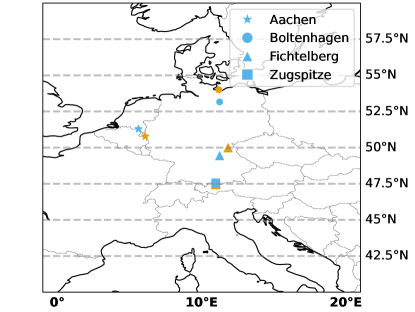
Figure A.1: Locations of German weather stations that serve as longer datasets in blue  . The corresponding CMIP6 locations we investigate for Figure 6 and Figure 8 are marked in orange  .

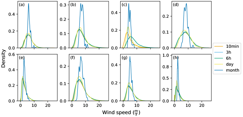
Figure A.2: Kernel density estimations of averaged wind speeds. The distributions of 10min, three-hourly, six-hourly and daily data look similar to a Weibull distribution; monthly data are not Weibull distributed.

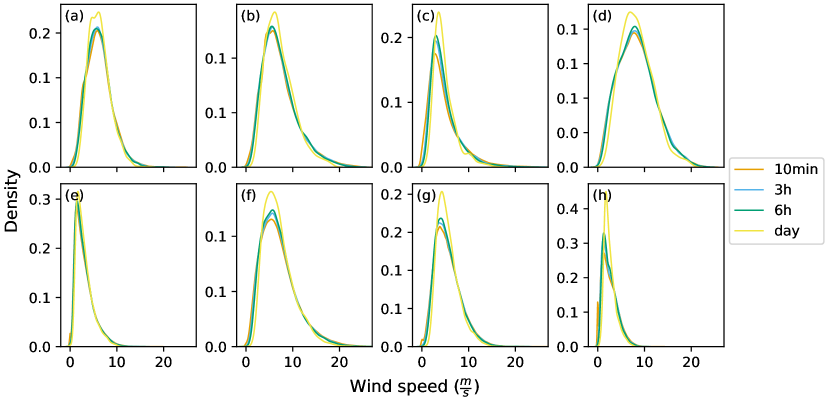
Figure A.3: Kernel density estimations of averaged wind speeds of different resolutions excluding monthly data.

Figure A.4: Kernel density estimations of instantaneous wind speeds of different resolutions. Data at most sites look approximately Weibull distributed.

Figure A.5: QQ-plots of averaged wind speeds and fitted Weibull distributions. From left to right the data resolution is 10min, three-hourly averages, six-hourly averages and daily averages.

Figure A.6: QQ-plots of instantaneous wind speeds and fitted Weibull distributions. From left to right the data resolution is 10min, three-hourly averages, six-hourly averages and daily averages.

Figure A.7: Figure 3 for longer datasets. Difference of cumulative densities from the 10min data to the other temporal resolution datasets for average wind speeds (left) and instantaneous wind speeds (right). It can be seen that the averaged wind speeds are visually distinguishable, which is less the case for instantaneous wind speeds, particularly for three- or six-hourly data.

(a) Absolute trends.

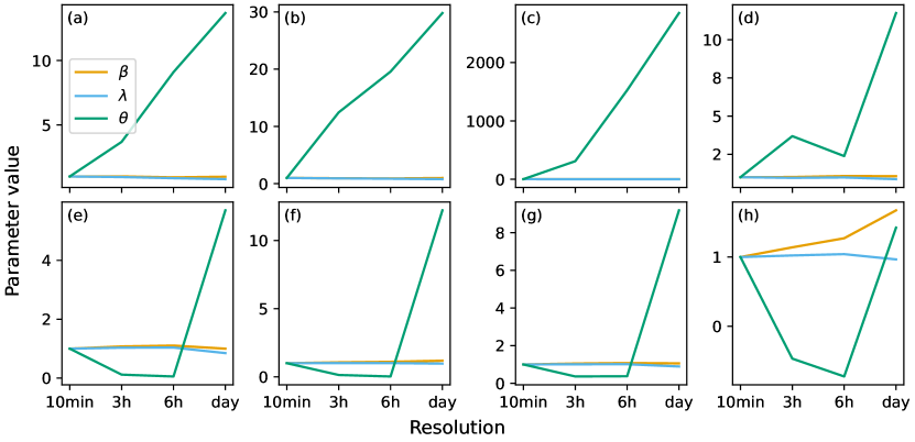
(b) Relative trends.

Figure A.8: Weibull parameter trends when fitted to averaged wind speed distributions.

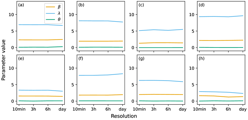
(a) Absolute trends.

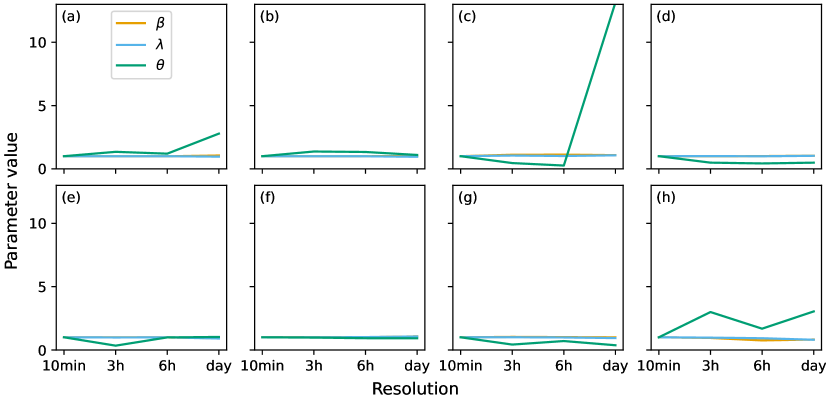
(b) Relative trends.

Figure A.9: Weibull parameter trends when fitted to instantaneous wind speed distributions.

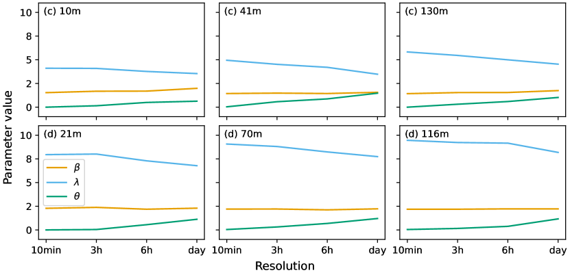
(a) Parameter trends fitted to averaged wind speed distributions.

(b) Parameter trends fitted to instantaneous wind speed distributions.

Figure A.10: Weibull parameter trends of different observations heights for the tall towers NWTC and Owez.

To test for robustness of our results we also use MLE to fit a generalized Gamma distribution

$$f(w;a,d,p)=\frac{\frac{p}{a^{d}}x^{d-1}\exp(-(\frac{x}{a})^{p})}{\Gamma(\frac{d}{p})}$$ (8)

with

$$\Gamma(z)=\int_{0}^{\infty}t^{z-1}\exp(-t)dt$$ (9)

instead of fitting a Weibull distribution. Both distributions were regarded to be suitable statistical models in earlier studies [e.g. Mert and Karakuş, 2015].

Figure A.11: QQ-plots of averaged wind speeds and fitted Gamma distributions. From left to right the data resolution is 10min, three-hourly averages, six-hourly averages and daily averages.

Figure A.12: QQ-plots of instantaneous wind speeds and fitted Gamma distributions. From left to right the data resolution is 10min, three-hourly averages, six-hourly averages and daily averages.

(a) Absolute trends.

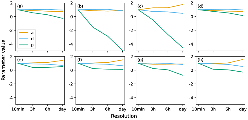
(b) Relative trends.

Figure A.13: Gamma parameter trends when fitted to averaged wind speed distributions.

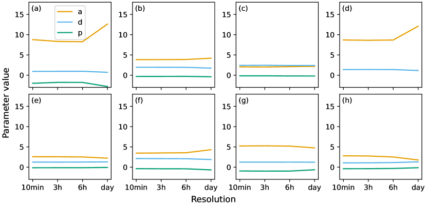
(a) Absolute trends.

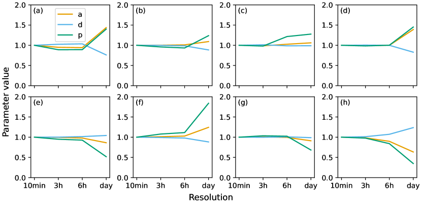
(b) Relative trends.

Figure A.14: Gamma parameter trends when fitted to instantaneous wind speed distributions.

	daily	six-hourly	three-hourly	10min
daily	1	$2.24\cdot 10^{-3}$	$4.30\cdot 10^{-5}$	$4.98\cdot 10^{-9}$
six-hourly		1	$\mathbf{4.54\cdot 10^{-1}}$	$6.88\cdot 10^{-6}$
three-hourly			1	$1.85\cdot 10^{-4}$

Table A.2: $p$-values of Kolmogorov-Smirnov test for averages Kelmarsh. All values where $p\leq 0.05$ are marked bold and the corresponding distributions are not considered to be significantly different.

	daily	six-hourly	three-hourly	10min
daily	1	$1.54\cdot 10^{-2}$	$5.58\cdot 10^{-3}$	$2.15\cdot 10^{-3}$
six-hourly		1	$\mathbf{1.00}$	$\mathbf{9.81\cdot 10^{-1}}$
three-hourly			1	$\mathbf{1.00}$

Table A.3: $p$-values of Kolmogorov-Smirnov test for instantaneous Kelmarsh. All values where $p\leq 0.05$ are marked bold and the corresponding distributions are not considered to be significantly different.

	daily	six-hourly	three-hourly	10min
daily	1	$8.15\cdot 10^{-11}$	$9.13\cdot 10^{-18}$	$1.35\cdot 10^{-33}$
six-hourly		1	$5.53\cdot 10^{-4}$	$2.51\cdot 10^{-35}$
three-hourly			1	$2.45\cdot 10^{-27}$

Table A.4: $p$-values of Kolmogorov-Smirnov test for averaged NWTC wind speed distributions. All values where $p\leq 0.05$ are marked bold and the corresponding distributions are not considered to be significantly different.

	daily	six-hourly	three-hourly	10min
daily	1	$\mathbf{1.64\cdot 10^{-1}}$	$3.84\cdot 10^{-2}$	$3.61\cdot 10^{-2}$
six-hourly		1	$\mathbf{7.21\cdot 10^{-1}}$	$\mathbf{6.20\cdot 10^{-1}}$
three-hourly			1	$\mathbf{9.01\cdot 10^{-1}}$

Table A.5: $p$-values of Kolmogorov-Smirnov test for instantaneous NWTC wind speed distributions. All values where $p\leq 0.05$ are marked bold and the corresponding distributions are not considered to be significantly different.

	daily	six-hourly	three-hourly	10min
daily	1	$3.00\cdot 10^{-3}$	$2.25\cdot 10^{-4}$	$1.40\cdot 10^{-5}$
six-hourly		1	$\mathbf{7.15\cdot 10^{-1}}$	$\mathbf{9.20\cdot 10^{-2}}$
three-hourly			1	$\mathbf{4.95\cdot 10^{-1}}$

Table A.6: $p$-values of Kolmogorov-Smirnov test for averaged Owez wind speed distributions. All values where $p\leq 0.05$ are marked bold and the corresponding distributions are not considered to be significantly different.

	daily	six-hourly	three-hourly	10min
daily	1	$\mathbf{2.14\cdot 10^{-1}}$	$\mathbf{2.18\cdot 10^{-1}}$	$\mathbf{1.29\cdot 10^{-1}}$
six-hourly		1	$\mathbf{1.00}$	$\mathbf{9.78\cdot 10^{-1}}$
three-hourly			1	$\mathbf{9.77\cdot 10^{-1}}$

Table A.7: $p$-values of Kolmogorov-Smirnov test for instantaneous Owez wind speed distributions. All values where $p\leq 0.05$ are marked bold and the corresponding distributions are not considered to be significantly different.

	daily	six-hourly	three-hourly	10min
daily	1	$3.83\cdot 10^{-14}$	$1.43\cdot 10^{-21}$	$3.24\cdot 10^{-52}$
six-hourly		1	$6.11\cdot 10^{-4}$	$1.76\cdot 10^{-45}$
three-hourly			1	$1.73\cdot 10^{-44}$

Table A.8: $p$-values of Kolmogorov-Smirnov test for averaged Aachen wind speed distributions. All values where $p\leq 0.05$ are marked bold and the corresponding distributions are not considered to be significantly different.

	daily	six-hourly	three-hourly	10min
daily	1	$2.89\cdot 10^{-22}$	$1.54\cdot 10^{-25}$	$2.14\cdot 10^{-28}$
six-hourly		1	$\mathbf{9.35\cdot 10^{-1}}$	$\mathbf{7.85\cdot 10^{-1}}$
three-hourly			1	$\mathbf{1.00}$

Table A.9: $p$-values of Kolmogorov-Smirnov test for instantaneous Aachen wind speed distributions. All values where $p\leq 0.05$ are marked bold and the corresponding distributions are not considered to be significantly different.

	daily	six-hourly	three-hourly	10min
daily	1	$4.47\cdot 10^{-23}$	$9.69\cdot 10^{-39}$	$2.71\cdot 10^{-72}$
six-hourly		1	$1.16\cdot 10^{-5}$	$3.01\cdot 10^{-45}$
three-hourly			1	$4.90\cdot 10^{-33}$

Table A.10: $p$-values of Kolmogorov-Smirnov test for averaged Zugspitze wind speed distributions. All values where $p\leq 0.05$ are marked bold and the corresponding distributions are not considered to be significantly different.

	daily	six-hourly	three-hourly	10min
daily	1	$5.68\cdot 10^{-22}$	$3.59\cdot 10^{-24}$	$3.84\cdot 10^{-27}$
six-hourly		1	$\mathbf{7.13\cdot 10^{-1}}$	$\mathbf{3.89\cdot 10^{-1}}$
three-hourly			1	$\mathbf{1.00}$

Table A.11: $p$-values of Kolmogorov-Smirnov test for instantaneous Zugspitze wind speed distributions. All values where $p\leq 0.05$ are marked bold and the corresponding distributions are not considered to be significantly different.

	daily	six-hourly	three-hourly	10min
daily	1	$9.77\cdot 10^{-34}$	$1.04\cdot 10^{-64}$	$1.39\cdot 10^{-85}$
six-hourly		1	$1.04\cdot 10^{-5}$	$1.69\cdot 10^{-44}$
three-hourly			1	$4.23\cdot 10^{-35}$

Table A.12: $p$-values of Kolmogorov-Smirnov test for averaged Boltenhagen wind speed distributions. All values where $p\leq 0.05$ are marked bold and the corresponding distributions are not considered to be significantly different.

	daily	six-hourly	three-hourly	10min
daily	1	$7.14\cdot 10^{-31}$	$1.72\cdot 10^{-34}$	$1.09\cdot 10^{-38}$
six-hourly		1	$\mathbf{7.84\cdot 10^{-1}}$	$\mathbf{3.59\cdot 10^{-1}}$
three-hourly			1	$\mathbf{1.00}$

Table A.13: $p$-values of Kolmogorov-Smirnov test for instantaneous Boltenhagen wind speed distributions. All values where $p\leq 0.05$ are marked bold and the corresponding distributions are not considered to be significantly different.

	daily	six-hourly	three-hourly	10min
daily	1	$4.20\cdot 10^{-108}$	$2.04\cdot 10^{-163}$	$3.60\cdot 10^{-265}$
six-hourly		1	$1.47\cdot 10^{-17}$	$1.64\cdot 10^{-187}$
three-hourly			1	$6.61\cdot 10^{-184}$

Table A.14: $p$-values of Kolmogorov-Smirnov test for averaged Fichtelberg wind speed distributions. All values where $p\leq 0.05$ are marked bold and the corresponding distributions are not considered to be significantly different.

	daily	six-hourly	three-hourly	10min
daily	1	$4.34\cdot 10^{-83}$	$2.06\cdot 10^{-117}$	$1.27\cdot 10^{-135}$
six-hourly		1	$9.02\cdot 10^{-6}$	$7.67\cdot 10^{-12}$
three-hourly			1	$\mathbf{4.24\cdot 10^{-1}}$

Table A.15: $p$-values of Kolmogorov-Smirnov test for instantaneous Fichtelberg wind speed distributions. All values where $p\leq 0.05$ are marked bold and the corresponding distributions are not considered to be significantly different.

Location	10min	3h avrg.	3h inst.	6h inst.
Aachen	0	-40.28	-3.47	1.99
Zugspitze	0	-39.16	4.76	6.06
Boltenhagen	0	-111.23	9.86	3.69
Fichtelberg	0	-62.71	1.83	-9.80

Table A.16: Errors (in $MW$) of wind power generation prediction when using 30 years of data of lower resolution (three-hourly average and three-hourly and six-hourly instantaneous) wind speed observations compared to 10min wind speed observations.

References

- Bañuelos-Ruedas et al. [2010] Fransisco Bañuelos-Ruedas, César Angeles-Camacho, and Sebastián Rios-Marcuello. Analysis and validation of the methodology used in the extrapolation of wind speed data at different heights. Renewable and Sustainable Energy Reviews, 14(8):2383–2391, 2010.
- CMIP6 data request [2016] CMIP6 data request. CMIP6 documentation, 2016. URL https://clipc-services.ceda.ac.uk/dreq/u/4b97609a32d53dff5b8e73729e4f258b.html. date accessed: 2023-07-07.
- Copernicus [2023] Copernicus. Decadal energy predictions, 2023. https://climate.copernicus.eu/decadal-predictions-energy.
- Courant et al. [1928] Richard Courant, Kurt Friedrichs, and Hans Lewy. Über die partiellen Differenzengleichungen der mathematischen Physik. Mathematische annalen, 100(1):32–74, 1928.
- Davy et al. [2018] Richard Davy, Natalia Gnatiuk, Lasse Pettersson, and Leonid Bobylev. Climate change impacts on wind energy potential in the european domain with a focus on the black sea. Renewable and sustainable energy reviews, 81(2):1652–1659, 2018.
- Dunn et al. [2019] Robert JH Dunn, Kate M Willett, and David E Parker. Changes in statistical distributions of sub-daily surface temperatures and wind speed. Earth System Dynamics, 10(4):765–788, 2019.
- Effenberger and Ludwig [2022] Nina Effenberger and Nicole Ludwig. A collection and categorization of open-source wind and wind power datasets. Wind Energy, 25(10):1659–1683, 2022.
- Eyring et al. [2016] Veronika Eyring, Sandrine Bony, Gerald A Meehl, Catherine A Senior, Bjorn Stevens, Ronald J Stouffer, and Karl E Taylor. Overview of the coupled model intercomparison project phase 6 (CMIP6) experimental design and organization. Geoscientific Model Development, 9(5):1937–1958, 2016.
- Giorgi and Gutowski Jr [2015] Filippo Giorgi and William J Gutowski Jr. Regional dynamical downscaling and the CORDEX initiative. Annual review of environment and resources, 40:467–490, 2015.
- González-Longatt et al. [2012] Francisco González-Longatt, Peter Wall, and Vladimir Terzija. Wake effect in wind farm performance: Steady-state and dynamic behavior. Renewable Energy, 39(1):329–338, 2012.
- Harper et al. [2010] Bruce A Harper, Jeff D Kepert, and John D Ginger. Guidelines for converting between various wind averaging periods in tropical cyclone conditions. 2010.
- Horvath et al. [2012] Kristian Horvath, Darko Koracin, Ramesh Vellore, Jinhua Jiang, and Radian Belu. Sub-kilometer dynamical downscaling of near-surface winds in complex terrain using WRF and MM5mesoscale models. Journal of Geophysical Research: Atmospheres, 117(D11), 2012.
- Jeong and Sushama [2019] Dae Il Jeong and Laxmi Sushama. Projected changes to mean and extreme surface wind speeds for North America based on regional climate model simulations. Atmosphere, 10(9):497, 2019.
- Jung and Schindler [2019] Christopher Jung and Dirk Schindler. Changing wind speed distributions under future global climate. Energy Conversion and Management, 198:111841, 2019.
- Kang and Won [2015] Song-Lak Kang and Hoonill Won. Intra-farm wind speed variability observed by nacelle anemometers in a large inland wind farm. Journal of Wind Engineering and Industrial Aerodynamics, 147:164–175, 2015.
- Kang and Won [2016] Song-Lak Kang and Hoonill Won. Spectral structure of 5 year time series of horizontal wind speed at the Boulder Atmospheric Observatory. Journal of Geophysical Research: Atmospheres, 121(20):11–946, 2016.
- Larsén et al. [2016] Xiaoli G Larsén, Søren E Larsen, and Erik L Petersen. Full-scale spectrum of boundary-layer winds. Boundary-layer meteorology, 159:349–371, 2016.
- Lopez-Villalobos et al. [2021] Carlos A Lopez-Villalobos, Osvaldo Rodriguez-Hernandez, Oscar Martinez-Alvarado, and JG Hernandez-Yepes. Effects of wind power spectrum analysis over resource assessment. Renewable Energy, 167:761–773, 2021.
- McVicar et al. [2012] Tim R McVicar, Michael L Roderick, Randall J Donohue, Ling Tao Li, Thomas G Van Niel, Axel Thomas, Jürgen Grieser, Deepak Jhajharia, Youcef Himri, Natalie M Mahowald, et al. Global review and synthesis of trends in observed terrestrial near-surface wind speeds: Implications for evaporation. Journal of Hydrology, 416-417:182–205, 2012.
- Mert and Karakuş [2015] Ilker Mert and Cuma Karakuş. A statistical analysis of wind speed data using Burr, generalized gamma, and Weibull distributions in Antakya, Turkey. Turkish Journal of Electrical Engineering and Computer Sciences, 23(6):1571–1586, 2015.
- Plumley [2022a] Charlie Plumley. Kelmarsh wind farm data, February 2022a. https://doi.org/10.5281/zenodo.7212475, date accessed: 2023-11-07.
- Plumley [2022b] Charlie Plumley. Penmanshiel wind farm data, February 2022b. https://doi.org/10.5281/zenodo.5946808, date accessed: 2023-11-07.
- Pryor and Barthelmie [2010] Sara C Pryor and Rebecca J Barthelmie. Climate change impacts on wind energy: A review. Renewable and sustainable energy reviews, 14(1):430–437, 2010.
- Pryor et al. [2018] Sara C Pryor, Tristan J Shepherd, and Rebecca J Barthelmie. Interannual variability of wind climates and wind turbine annual energy production. Wind Energy Science, 3(2):651–665, 2018.
- Ramon et al. [2020] Jaume Ramon, Llorenç Lledó, Núria Pérez-Zanón, Albert Soret, and Francisco J Doblas-Reyes. The Tall Tower Dataset: a unique initiative to boost wind energy research. Earth System Science Data, 12(1):429–439, 2020.
- Ramon et al. [2022a] Jaume Ramon, Llorenç Lledó, Núria Pérez-Zanón, Albert Soret, and Francisco J Doblas-Reyes. Owez wind farm data, 2022a. https://talltowers.bsc.es/node/4856, date accessed: 2023-11-07.
- Ramon et al. [2022b] Jaume Ramon, Llorenç Lledó, Núria Pérez-Zanón, Albert Soret, and Francisco J Doblas-Reyes. NWTC wind farm data, 2022b. https://talltowers.bsc.es/node/4846, date accessed: 2023-11-07.
- Ringkjøb et al. [2020] Hans-Kristian Ringkjøb, Peter M Haugan, Pernille Seljom, Arne Lind, Fabian Wagner, and Sennai Mesfun. Short-term solar and wind variability in long-term energy system models-A European case study. Energy, 209:118377, 2020.
- Rinne [2008] Horst Rinne. The Weibull distribution: a handbook. CRC press, 2008.
- Scott [2015] David W Scott. Multivariate density estimation: theory, practice, and visualization. John Wiley & Sons, 2015.
- Shin et al. [2018] Ju-Young Shin, Changsam Jeong, and Jun-Haeng Heo. A novel statistical method to temporally downscale wind speed Weibull distribution using scaling property. Energies, 11(3):633, 2018.
- Soares-Ramos et al. [2020] Emanuel PP Soares-Ramos, Lais de Oliveira-Assis, Raúl Sarrias-Mena, and Luis M Fernández-Ramírez. Current status and future trends of offshore wind power in europe. Energy, 202:117787, 2020.
- Stull [1988] Roland B Stull. An introduction to boundary layer meteorology, volume 13. Springer Science & Business Media, 1988.
- Tawn and Browell [2022] Rosemary Tawn and Jethro Browell. A review of very short-term wind and solar power forecasting. Renewable and Sustainable Energy Reviews, 153:111758, 2022.
- Tobin et al. [2015] Isabelle Tobin, Robert Vautard, Irena Balog, François-Marie Bréon, Sonia Jerez, Paolo Michele Ruti, Françoise Thais, Mathieu Vrac, and Pascal Yiou. Assessing climate change impacts on European wind energy from ENSEMBLES high-resolution climate projections. Climatic Change, 128:99–112, 2015.
- Tobin et al. [2016] Isabelle Tobin, Sonia Jerez, Robert Vautard, Françoise Thais, Erik Van Meijgaard, Andreas Prein, Michel Déqué, Sven Kotlarski, Cathrine Fox Maule, Grigory Nikulin, et al. Climate change impacts on the power generation potential of a European mid-century wind farms scenario. Environmental Research Letters, 11(3):034013, 2016.
- Van der Hoven [1957] Isaac Van der Hoven. Power spectrum of horizontal wind speed in the frequency range from 0.0007 to 900 cycles per hour. Journal of Atmospheric Sciences, 14(2):160–164, 1957.
- Von Storch [1999] Hans Von Storch. On the use of “inflation” in statistical downscaling. Journal of Climate, 12(12):3505–3506, 1999.
- Wang et al. [2019] Yun Wang, Qinghua Hu, Linhao Li, Aoife M Foley, and Dipti Srinivasan. Approaches to wind power curve modeling: A review and discussion. Renewable and Sustainable Energy Reviews, 116:109422, 2019.
- WCRP CMIP6 [2023] WCRP CMIP6. ESGF data node, 2023. https://esgf-data.dkrz.de/search/cmip6-dkrz/, date accessed: 2023-27-07.
- [41] Deutscher Wetterdienst. Open data german meteorological service. https://opendata.dwd.de/climate_environment/CDC/, date accessed: 2023-07-11.
- Yang et al. [2022] Yuchen Yang, Kavan Javanroodi, and Vahid M Nik. Climate change and renewable energy generation in Europe—long-term impact assessment on solar and wind energy using high-resolution future climate data and considering climate uncertainties. Energies, 15(1):302, 2022.