Relativistic Propagators on Lattices
Abstract.
I define the lattice propagator on a very general collection of graphs, namely graphs locally isomorphic to . I then define polygonal approximations to the minkowski metric and define a corresponding lattice propagator for these. I show in , as suggested by the metric approximation, the continuum limit of the polygonal propagators converges to the Klien Gordon Propagator. Finally, I obtain the taxicab polygonal propagator in a very general collection of spaces, including , the Klein bottle, and a discretization of de-Sitter space.
1. Introduction
This paper aims to define the propagator of QFT (Quantum Field Theory) in terms of geometrical quantities, as per the original intuition of Feynman. Feynman’s original derivation of the path integral formulation of the propagator expressed it in terms of a limit of oscillatory integrals [5], but there are mathematical problems in making this expression rigorous in its most general setting. The path integral as a measure on paths works in the setting of Statistical Mechanics in the Kac-Feynman formula [8], but attempts to do the same in the setting of propagators have lead to candidate measures that are not -additive [1]. Other attempts to make the path integral rigorous include treating it as a functional that converges on a family of well-behaved functions [1] and using Gaussian free fields to define the propagator in the setting of Conformal Field Theory [11]. Most approaches are highly abstracted from treating the path integral as a phase-weighted sum over paths in space. This paper aims to develop another approach that centrally employs this intuition.
In Section 2, I define a discrete propagator as a complex-valued function on pairs of vertices in a discretization of space. The function itself is a sum over achronal local paths (defined in Section 2) weighted by a phase whose angle is the minkowski length of those paths. Because these quantities are finite, I don’t need to worry about convergence issues that plague most formalizations of propagators. I obtain analytic expressions for these propagators and then show that these analytic expressions converge to a continuum limit as ultra-fine lattice lengths are considered. This employs recent work in continuous lattice path counting in [2] and [21] where a continuous multinomial coefficient is defined (another result of this work is that this coefficient is a well defined, fully differentiable function). To show that the objects I obtain are indeed discretizations of the QFT flat-space free scalar propagator, I use transformation invariance arguments. I show that any sup norm limit of lattice path integrals (as more directions on the lattice that paths are allowed to occupy are included) converge to the closed-form expression for the QFT propagator.
I must direct some of this introduction towards polygonal minkowski metrics. Put plainly, a polygonal metric is any metric whose unit sphere is a polyhedron. We need to make use of these metrics as the action of a relativistic bosonic particle is related to an integral over a path of its normal minkowski length. We will need a discretization of the minkowski metric to define our discrete propagators.
The most well-known polygonal metric is the taxicab metric on Euclidean space; its associated perimeter shows up as the free energy of many Ising model solutions [7],[4]. In this paper, I will show that a minkowski taxicab metric is the first among a series of metrics that converge to the minkowski one. This family of polygonal metrics has an interesting relationship to Pythagorean triples [18], which I develop in Section 6. I show for the continuum propagators for converge to the minkowski propagator as , thereby motivating the idea that the taxicab propagator is a ’first order’ approximation to the more difficult minkowski propagator. Finally, I demonstrate the versatility of the taxicab minkowski propagator.
I show that lattice propagators can be calculated on discretizations of general orbifolds. I will also work with a tropical formulation of de-Sitter space [14],[13]. I obtain continuum propagators for these settings. I also derive that the taxicab metric propagators on de-Sitter space are ignorant of compact dimensions, but the propagator probes these dimensions well in flat space. Finally, I mention that all the propagators I obtain in this work will correspond to free particles without interaction terms. Interactions are difficult to express geometrically without more complicated theories (like String theory [22]). Generalizing the taxicab propagators in the setting of strings and membranes will be the subject of latter work.
2. Notations and Statement of Theorems
Let and . I define . The first copies of are defined as the spatial coordinates and the last with time. I note that , so it has a boundary in . I will constrain ourselves to such that . I can therefore give an arbitrary equivalence relation which partitions into pairs. I shall leave completely general. I may also consider drawing X from a tropical polynomial context. Let . Then, I define an arbitrary tropical polynomial as the following:
| (1) |
I will occasionally let . In the case of these X’s I may have to specify what coordinates are time and spatial, though unless explicitly stated, it will be that convention induced by . Our definitions will generally hold for all the above-described .
If , then is the projection of into the time coordinate (and I will denote as any space coordinate projections). I give the graph structure where are its points and . This has a metric given to it by the graph distances. Let . I define on the following functions
| (2) |
For all our purposes, I will only be using on . The first equation in Equation 2 is clearly the metric on . The subscript in the second is used to denote its similarity with the metric; it is the analog of the minkowski metric in our setting. I will therefore refer to the second part of Equation 2 as the minkowski metric. Let . Consider the set of scaled primitive pythagorean triples with hypotenuse below n, namely . The word primitive places an extra constraint on such that if we consider the equivalence class placed upon these vectors by parallelism, then we only keep the representative with the lowest hypotenuse. These points have a natural ordering from least x coordinate to most; let us denote as the i-th vector under this ordering. For , then, we may define Equation 3 as our polygonal minkowski metric.
| (3) |
For , we define as . These are functions , and they are meant to be natural polygonal approximations of the minkowski metric. One can see this via Figure 7. When , this becomes , or the taxicab minkowski metric. I can extend this metric to high dimensions as Ill in Equation 4.
| (4) |
I shall return back to Equation 2 and Equation 3 for a moment. Let’s define . A subset is called generating iff for all there is such that . Then an axes of symmetry of , denoted , is some such that if and then . So, every direction has a unique representative. The double usage of for scaled Pythagorean triples and as axes of symmetry of will be shown to not be an abuse of notation in Theorem 12 (except the axes of symmetry of will include also light paths). Our language in this paper will suggest that this set is unique to each we will not prove this for we do not require it for the next concepts.
I define as a path as set such that . Then, our achronal, local paths between and as the following:
| (5) |
I define our achronal, local polygonal paths between and as the following:
| (6) |
On and we place an equivalence relation on paths; two paths are equivalent if their indexing set traces out the same piecewise linear paths in . The use of axes of symmetry is made clear in this context; each equivalence class in has a unique representative with difference sequence drawn from (Theorem 14).
Clearly, from Equation 5 and Equation 6 I have . Let . Then I define the polygonal and minkowski proper time in Equation 7.
| (7) |
From this definition, I immediately obtain Theorem 12. These geometrical results are developed because I will be viewing the path integral as a geometrical object. For this purpose, I define the following functions and . Let .
| (8) |
These functions are our discrete propagators. They are the main subject of study in this paper.
These are all our basic definitions in the discrete context. I will devote some of our paper to the continuous setting. For this, I must define for our original X a natural domain , which is the result of taking infinitely fine lattices. In the first context (non tropical), it’s with an associated equivalence relation on pairs of points in as a subspace of . I note that if is the definitional tropical polynomial of , then can be immediately extended to . will then be the zero set of this extended . I now want a generalization of the closest integer function . For I let be the closest point in the range to the domain under the metric.
Then our generalization is defined as in Equation 9.
| (9) |
Finally, for those which have some finite element in their definition, I must also change their dimensions to approach as a limiting space for infinitely fine lattices. Therefore, when I write , or , I am referring to those objects for when .
We will find that recent developments in combinatorics, mentioned in Section 1, facilitate the expression of continuum propagators in all of these settings. Counting lattice paths are naturally connected to the multinomial coefficient, and therefore continuum propagators seem to require the development of a continuous multinomial coefficient. As defined by Cano and Diaz in [2], and later generalized by Wakhare, Vignat, Le, and Robins in [21], we consider the continuous multinomial coefficient in Equation 11 for l variables. Let , denote the Lebesgue measure on [6], and for denote by the number of Smirnov words of length n and N [21]. Furthermore let , let denote singular letters of our Smirnov word taking elements among some collection of d dimensional vectors, and let denote these vectors. For we define the path polytope in Equation 10.
| (10) |
We now have our desired definition of the continuous multinomial in Equation 11:
| (11) |
Problematically, the continuous multinomial was never shown by either [2] or [21] to converge except in special cases. The necessary convergence results are developed in Section 6; we will also show more rigorously in what sense they are continuous analogs of the discrete multinomial coefficients. Namely, for we introduce the operator in Equation 13. This operator acts on sums indexed over paths in . Let be some path indexed complex valued function and let be its radial and angular components. Let denote the number of distinct linear segments in . Then, we can rearrange any general sum over as done in Equation 12.
| (12) |
Then, we may write easily in this context (in Equation 13)
| (13) |
As demonstrated in Theorem 10, this operator is required to connect a natural estimate of counting paths to a notion of volume, as one would expect in the continuous setting. With all the relevant concepts defined, the following continuum propagators are defined in Equation (in the event they exist)
| (14) |
In Equation 14, we will be satisfied if the sequence of has a convergent subsequence towards some function in a pointwise or sup norm sense, and therefore that this limit is unique w.r.t limits. I now move on to the statement of our theorems. I aim to demonstrate that and can be defined and calculated in any of the I defined above, that in some sense, and that and exist in a very general context and that . I aim to show that can be identified with the free particle propagator from Quantum Mechanics and that this is why I should even care about .
I then show that and has a remarkable ease of computation in all . These latter theorems represent the bulk of our work; the former serve to motivate the latter. Let us first state the motivating polygonal propagator theorems, and then move on to working with and
2.1. Statement of Theorems
We first derive an analytic expression for .
Theorem 1.
Let . For we have
| (15) |
and we have equal to Equation 16 up to a multiplicative normalization constant dependant only on t.
| (16) |
Next, I want to demonstrate the capacity of to approximate . For that we first show that a limit of the continuum propagators exists. For this we have Theorem 2.
Theorem 2.
Consider the expression in Equation 17 for
| (17) |
This expression shows that the sequence of continuum propagators is Cauchy in the sup norm (so long as the maximum t to evaluate this inequality is constrained). Therefore, it has a convergent subsequence, and exists.
It will become clear from Theorem 1 that not only exists, but is non-trivial. In the context of [15], we will conjecture that this limiting function is the KG propagator and not the physically significant Feynman propagator. We wish to motivate our work by relating it to physical quantities; i.e. rigorously defining the physically meaningful propagators. To this end, we instead obtain the following theorems for Feynman propogators. We define (as the Feynman propogator ) the same discrete sum as in Equation 8 except we allow the to be the sum of difference sequence elements of both for . As we will see in Lemma 2, this will reveal some beautiful symmetries underlying the Feynman Propagator.
When we obtain the continuum object , there is another change in convention we must adopt to obtain Theorem 3 relating to normalization. The aim of the divisor used in Equation 14 was to normalize the propagator such that its inverse Fourier transform would have a fixed integral. This becomes problematic as in the proof of Theorem 3 we would need to normalize a non-normalizable function; we would for the solution a propagator which had deltas along . Therefore we adopt the following convention for our divisor. We shall find each , defined up to some time-dependent normalization, has a well-defined inverse Fourier transform in mass by Theorem 1. The normalization adopted will be to multiply the regular normalization by some power of t, effectively leaving unconstrained the integral but constraining its pointwise value.
Let denote the zero-th Bessel function of the second kind, we know from [9] that it is the form of the relativistic bosonic propagator , and we derive it rigorously within Theorem 3.
Theorem 3.
Let . For we have
where is a fourier transform C’ can possibly have a phase and then by definition
Now that we have established theorems that motivate the utility of our lattice propagators, we move to the propagator. This propagator is simple to compute in many contexts and allows for the study of the first-order properties of propagators on an arbitrary surface.
A note for physicists
The nuance explained before the statement of Theorem 2 applies to the section below. These results do not approximate the time ordered Klein Gordon propogator [15] and the realistic . To replicate this as we have done in Theorem 2, we would also need to include in negative length terms. This is akin to considering anti-particles and permitting the spontaneous alteration of a particle to an anti-particle during its travel.
2.2. Statement of Theorems
First, I find analytic formulas for the propogator for . We will find non-implicit expressions for for arbitrary d and show how we would obtain the continuum limit for only .
Theorem 4.
Let such that . Furthermore, let denote the taxicab norm on X. Then for . I have
| (18) |
Letting we have
| (19) |
where denotes the fourier transform.
I now will calculate for equivalence classes such that and the Klein Bottle. Future work will be devoted to an in-depth treatment of all that lead to Riemann Surfaces in . Theorem 5 details our results for the torus.
Theorem 5.
Let and let all . Furthermore, let be defined on such that if there is some st and for all . For ease of expression, we will denote as the for this and for the expression derived in Equation 18. Then we have Equation 20.
| (20) |
We have the result for the Klein bottle in Theorem 6. This surface is non-orientable, so technically not a Reiman surface.
Theorem 6.
Let and let all . We let be defined on such that if such that and or and . For ease of expression, we will denote as the for this X and for the expression derived in Equation 18. Then, we have
| (21) |
Finally, I want to include one result for X in the context of tropical surfaces. Let and let . Then, . One may recognize that this surface is the tropical equivalent of de-Sitter space for . There are tropical versions of each de-Sitter space; for now, we will also let be the zero set of for any .
Theorem 7.
Let be the zero set of (at this is a tropical surface for . Say such that and . Then we have Equation 22.
| (22) |
We also obtain . It immediately arises from [21].
| (23) |
I now move on to proving these theorems.
3. Proofs of the Theorems
First, let us obtain the proof of Theorem 1
Proof.
We let such that . Let be as derived in Theorem 12. For , we know by Theorem 14 that ’s difference sequence may be drawn from ; let be the number of elements of the difference sequence of equal to . Then, we note that for any path the following properties hold:
-
•
-
•
-
•
Let us denote as for the moment and attempt to group together paths of the same phase. For a fixed phase I, we have different ’positions’ we may place our vectors from . We must place of these into the collection for , into the collection for , etc. Namely, once we find a distinct combination of which satisfy , we have different possible paths. Altogether, this means we obtain a propagator takes on the form
| (24) |
We now want to remove the implicit conditions . To do so, we recognize that . We order such that is that which corresponds to the in Theorem 12, , and the order on the indeces is for . We know that corresponds to because it is always in and must be in the center of the set by symmetry. First, to generate a path, we may allow be any positive number below (as before we have written anything else, this variable is unconstrained). Then, the bounds on as defined in Eq 27 follow for as we just enforce condition and on the partial sums. With this convention established, our conditions become the bounds of Eq 27 and of Equation 25
| (25) |
where we satisfy Eq. 25 last after fixing each for . Solving the last two of these expressions, we have Equation 26.
| (26) |
Giving us the final near desired expression of Eq 27.
| (27) |
This expression is correct barring a caveat: we must enforce the condition that Eq 26 are non-negative integers. The first term is clearly an integer, and if we draw our as in Eq 27, it will be positive because of our upper bounds on each . We note the other two terms are either both integers or both half integers. The expression is the same regardless of the by the symmetry of , so it will not change the parity. The only other difference in the terms is the first two parts, which are of the form . This is the same number mod two, so either are both odd or even. Furthermore, let , then , so this all depends on being positive and even. We will let that remain our only implicit condition. Now, let’s look at what applying does. Our commutes past our sums over and applies directly to the multinomial coefficient. This is because said sum just determines how many of each element in is in our path, and then the multinomial coefficient contains the contributions from each different segment numbered path for the said combination of elements. Let . We obtain Equation 28.
| (28) |
From Equation 28 we can try to write down an expression for .
| (29) |
As is done in Theorem 4 for , we absorb into the numerator and denominator. And just as was done there, we note that the denominator converges to some integral over a continuous multinomial coefficient, which is finite by Theorem 11. That leaves us to consider the numerator. Let . In the theme of Theorem 4, if the maximum of the multinomial in Equation 29 lies in the constraints of Equation 29 and if we have infinitely large magnitude I we sum over, then this converges to Equation 30, the well-defined function from
| (30) |
We note from our discrete sum over reaches arbitrarily high bounds. Since the continuous multinomial is rapidly decaying for small I and growing for large, this tells us we get the entire integration range for our integral. Similarly, we note the upper argument of the continuous multinomial can be expressed as , which is bounded by and so our function is Schwartz class by Theorem 11 and has a defined Fourier transform.
∎
Now that we have obtained , let us obtain a proof showing that , i.e. Theorem 2
Proof.
To begin, we want a function that will let us see paths in as approximate paths in for . This approximation will let us constrain the difference between continuum propagators. Let’s define the function as follows. Let , and consider the set . This set has at most two vectors; if it contains one, we let be said vector. If it has two, we let be the vector of the two with least . This gives us a well-defined function between our individual steps. Clearly, this extends to by applying to the unique difference sequence of in (given by Theorem 14) to obtain a different sequence of a new path, denoted .
Let be vectors aligned with and , respectively, but such that . Then, as it is necessarily the case that . This is because we know that there are asymptotically circularly equidistributed points in and in (by the circle equidistance Theorem 15), meaning that by the infinum definition of , each vector in is in and distance from its image under in and that . Let denote the number of difference sequence elements of . This second fact implies that as the preimage of includes for every difference sequence element a point in of said difference sequence element.
Let us define as in Equation 31. We will define in the next paragraph
| (31) |
Consider Theorem 10. The continuous multinomial coefficient has a peak when all of its arguments are equal to their sum divided by and exponentially decays outside that range. Furthermore, when all the coefficients equal their sum divided by l, the Gaussian term becomes 1, and we are left with . By the work in Theorem 1 we know equals where is the weighted average of the time increment in each walk. Because each will concentrate on being equally expressed, is the average time increment of unit vectors along directions in ; it is a constant function of indepednent of t and the linear segments in the directed paths the continuum multinomial expresses. By rearrangement this equals . By substitution, this means the maximum of for time is Equation 32.
| (32) |
Equation 31 we use in the denominator of to normalize it, as paths would grow on the order as there would be an average time spent in line in the directed path and directions for each line to take by the asymptotic property of pythagorean triples (Theorem 15). We’ve shown that the continuum limit under of grows as or for an average time of each step in a directed path. This would imply that . Our same proof above allows us to conclude that and we note so . These last steps hold approximately around the sharp maximum of the continuum multinomial coefficient, where Stirling’s Approximation may be used to find the subleading terms in and .
These two tools allow us to approach our Cauchy claims. Consider first the terms in Equation 33:
| (33) |
We obtain Equation 33 by the Triangle Inequality. We note that some perimeters are equal ( for a difference sequence of ), so the first and second terms immediately disappear. Now, say where , and is allowed to vary. Then, we can add and subtract a term to obtain Equation 34.
| (34) |
We can modify the first term of Equation 34 to obtain Equation 35. To obtain this expression, we note that ; so, while we originally had a sum over elements of , we can rearrange our sum grouping together all that are mapped to the same element . This results in the cardinality of the preimage of a path being present in Equation 35.
| (35) |
If we demonstrate that if when we take , this expression will disappear. This follows from our calculation of leading order approximations of and that we found above. Let us constrain the second expression of Equation 34; we do so in Equation 36.
| (36) |
Here we make the observation that to obtain Equation 37.
| (37) |
where is a uniform bound on the difference of and . We know each vector is can be chosen to be uniformly separated from each other in norm by , and is absolutely continuous with (not visa versa as null-like vectors can have quite different and equal ). We bounded and in the work above; this demonstrates the result.
∎
We want to provide Lemma 2, whose importance to this proof allows it to be excluded from the definitional proofs of Section 6. To use and even prove lemma 2 effectively, we must relate it to the continuous multinomial of Equation 30. For this, we require a more tautological lemma in the form of Lemma 1. Let such that and consider the paths to composed of a difference sequence among in Equation 38.
| (38) |
We note that is defined so that its points are uniformly distributed across the surface (in direction atleast; in magnitude we are incapable of doing so due to it being non-compact). Consider , the set of Smirnov words of length n and p many letters. We can associate to each letter in these Smirnov words a direction in . Let for Lemma 1 denote the length obtained from on a path in (paths whose sets lie in ) where is the metric whose axes of symmetry are
Lemma 1.
Consider the function in Equation 39
| (39) |
All portions of Equation 39 are as they defined in [21], referred to in Section 1, and rigorously shown to exist in Section 6. Here, represents a Smirnov word of length with p letters, and is the polytope of directed paths from to corresponding to that word with steps from . Then, if we let denote the set of vectors in except , and if is the polygonal metric whose axes of symmetry is , then is equal to the argument of the Fourier transform in Equation 30 with the appropriate substitutions and (with ) divided by the denominator of Equation 39.
Proof.
We can show that the two desired expressions are equal by showing they are the same limit of of some discrete propagator-like object. Consider Equation 40.
| (40) |
These are all the points in that can be approximated by some finite sum of elements in ; we label it to indicate it will only be used temporarily in the context of this proof. This space is isotropic like our original domain of in that any point may be treated as and you will still get the same points obtained from step-wise paths in (just translated). Because for all has , the natural extension of the definition of to this setting still obtains some finite collection of discrete paths. Similarly, we also would obtain a polygonal minkowski metric (call it ) from the same Equation 3, and from it, we could define . To define in this setting, we need to define for what the closest point function is. We may say:
This arg-min exists because the topology induced on by is discrete; this fact is implied because each point in must be achieved in finite time from some base point using steps st . These are all the notions we need to define , and finally, if we replace with throughout all the steps of Theorem 1, then we also would obtain as the expression we find in the hypothesis of this lemma. Now, we show has, as the argument to its Fourier transform, something that is equivalent to the polytopic sum of Lemma 2. In Theorem 10, we see that all we need to show is that the discrete paths of with some number of linear segments can be understood as discrete points lying in some continuum polytope (then because polytopes are Riemann integrable, the same arguments of Theorem 10 work in this setting). If we consider some Smirnov word composed of letters from and length l, all of which describe one of the polytopes in the polytopic sum of Lemma 2, then we get that said polytope is a dimensional polytope embedded in . We see this in Figure 1.
In Figure 1, we see an approximate lattice path to the directed one. It is clear from the figure that the integer coordinates of this lattice path would lie inside the polytope with l linear segments adjoining to (the polytope would include all integer paths adjoining and among its collection of direct paths). As we scale said polytope to larger sizes, it is still the case that the lattice paths between two points would be among the paths constituting the path polytope. The arguments of Theorem 10 proceed thereafter to obtain the desired result.
∎
For words with letters among , we have a mapping ; this mapping takes to and is equivalent to rotating the underlying vectors by radians. If we let indicate the operator which rotates some by , then induces a volume preserving mapping from and .
From this we have Lemma 2.
Lemma 2.
Sneaky Trick
Consider the function in Equation 39. Again, all portions of Equation 39 are as they are defined in [21], referred to in Section 1, and rigorously shown to exist in Section 6. Here, represents a Smirnov word of length with p letters, and is the polytope of directed paths from to corresponding to that word with steps from . Then, a sup norm cluster point of the sequence exists and equals .
Proof.
| (41) |
We know is bijective on words ; hence, we can reorder terms in our sum between the first and second lines in our above equation depending on what maps to. If we apply to every word throughout the whole sum, it will change into the same volume path polytope to and revert giving us . So, is invariant under the rotation group isomorphic to , and any limit of it would be invariant under the rotation group on the first two coordinates and be a function of .
Let now denote and let denote the velocity obtained from iterating the einstein velocity summation formula (Eqaution 42) times using the same incremental velocity .
| (42) |
| (43) |
In the last line of Equation 43 we create the sets and . These are the subset of Smirnov words from our original alphabet of that must include the last directions for nor the first for .
We note that naturally induces a volume-preserving association between and , and we have subtracted those terms away to obtain the last line of Equation 43. maps those directions outside of to directions wholely outside of ; it must have a restricted domain to be a proper map between two sets of words. It is for this reason that the only terms left in the sum in Equation 43 lie outside the domain and image of (and it is in this manner and obtain their definitions).
This last line has the upper bound . The denotes the average volume of the path polytope over the Smirnov words in and . The numerator of this fraction is less than the denominator (by its sup definition). As increases (with ) the fraction will approach zero. This is because is proportional to the total number of Smirnov words without the extra constraint that they have some letter in their composition, and this extra constraint means that is times as large as or . Looking at a word in and , we can find the letter it is forced to have. By substituting this letter with the other directions in we find there are more words in the composition of than . An important thing to note is that as increases the remains invariant w.r.t p.
Since constitutes a macroscopic boost, we have demonstrated that at large is approximately boost invariant, not . Since only depends on time, however, we have shown that a limit of has its dependence on x enveloped as a dependence on and therefore it is a function of . Namely, the limit over p of must be of the form , where is constrained by our normalization factor.
Say that the variable has a distribution as governed by that tends towards uniformity in the interval . Then we note (from ) that is distributed in the desired manner on the domain (from the Radon-Nykodym derivative of measures on ). The quantity is the angle of paths drawn from ; due to the p-fold rotational symmetry of we obtain the desired uniformity at . We have the desired result.
∎
Now, the main motivating theorem we will provide in this document is Theorem 3. We prove this now:
Proof.
First, we derive . Note that we are just allowing in Theorem 1 for the vectors in to have negative phases. Let denote the set of pairs where denotes whether we associate to the length . Then, for indexing is the number of steps in devoted to the pair . We are purposely re-indexing our array here because our expression in Equation 44 becomes unwieldy otherwise. All the same proof of Theorem 1 shows that is equal to the expression in Equation 44.
| (44) |
Note that the expression for Equation 44 is almost identical to Equation 30 with the exception of the inclusion of indices. As a sanity check, is finite and defines a compact domain of integration and the denominator of our continuous multinomial less than as expected. A barely modified proof as to what was employed in Theorem 3 serves to demonstrate after this that the pointwise limit of exists and is non-trivial. We now want to use Lemma 2 to complete the derivation of , namely that the two sequences and that used in the statement of Lemma 2 converge to the same limit.
For this, we note that and the directions in the polytope of Lemma 2 for are both equidistributed on the sphere by Theorem 15. The expression in Equation 30 is continuous w.r.t the directions in used to construct it; therefore, if we took a sequence of the difference point-by-point of the argument of the Fourier transform of Equation 30 for the original and those directions in Equation 38 for , we obtain a sequence which goes to zero (by equidistributedness of pythagorean triples these directions ultimately approximate each-other).
There are a couple of steps before we can employ Lemma 2. First, we note that our above work, along with Theorem 2, demonstrates that Equation 30 has a sup norm limit for the directions in Equation 38. We now only need to show that the argument of Equation 30 is equivalent to the expression in the hypothesis of Lemma 2. This last proof is performed by Lemma 1.
∎
4. Proofs of the Theorems
Let us state the proof of Theorem 4:
Proof.
Let . Then, we can take where is a unit direction in . This is because by Theorem 14 any path in can be generated by the elements of and by Theorem12 is the set above. We will denote by the number of elements in the difference sequence are for . Let’s also denote by the number of elements that are Then, we must have the following for to end at :
-
•
-
•
Since , the phase is only determined by . In other words, . We will let so that is our phase. From the second condition on our we know that the number of different sequences must be one less than the time coordinate because each element of increments our path by 1. So . The number of paths with a fixed phase and these properties is a simple multinomial; the number of ways to sort points into our and . So we have Equation 45
| (45) |
In deriving our multinomial in Equation 45, we must also recognize that possibly different can satisfy our initial constraints and include a sum over them. Using our second condition (and the fact that this becomes
| (46) |
We note that condition of Equation 46 can be rewritten . For this, however, we will obtain non-integer values should . This corresponds to no path being possible between these two points, hence the inclusion of in our final expression. The condition on the sum (and each ) leads to the expansion and our result; we sum over all allowed first, and then with a choice of all allowed , etc. This will yield every combination consistent with our equations and the expression desired for Theorem 4. Now, let . Then, for we have
| (47) |
Using Sterling’s formula we obtain Equation LABEL:equation:Stirling.
| (48) |
Upon taking a derivative, we obtain Equation 49.
| (49) |
We note up to first order, this expression equals , which has the zero located at in Equation 50
| (50) |
Using the continuous multinomial distribution concentration property found in Theorem 11, we know that concentrates about with dramatically vanishing terms outside of . Our phase converges to the same constant value over these non-negligible terms because we divide by in its argument. This implies that
| (51) |
We can multiply the numerator and denominator (which will behave similarly sans phase) by n, and then this sum (by the definition of a Riemann integral) converges to some normalized Fourier transform of the continuous multinomial in terms of the variable I to in Equation 52. This is because the bounds of our sum contain the sharp maxima of the continuous multinomial at between and ; therefore, this integral amounts to all of the integral required for the Fourier transform.
Note that in the denominator the factor of acts on a sum very much like the numerator but without a phase. This will obtain an integral of the continuous multinomial, but by Theorem 11, we know this is integrable, and we can absorb it into some .
| (52) |
By Theorem 11, we know this Fourier transform exists. This is worked out in detail. Similarly, the discrete propagator for all the other cases becomes Fourier transforms, and as the above work shows, we need only show that the peak of the continuous multinomial lies in our sum bounds (more rigorously that is within from the boundary of the continuous region). That would give us Equation 53.
| (53) |
∎
With for obtained in Theorem 4, we may use it to obtain any Riemann Surface, which has a simple universal cover in . We will perform the proofs of Theorem 5 and Theorem 6 simultaneously using their well-known covering by in the following paragraphs.
Proof.
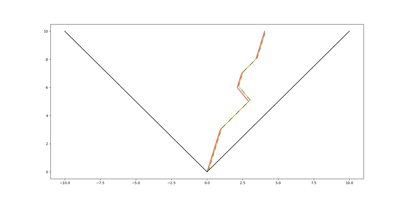
The covering takes to its representation such that there is some where . If we want to describe some for , it’s sufficient to see how the paths raise in . These will be paths from some element of to another of . These would over-count the paths between and in the original ; we want to fix a representative in the cover of our origin point. Then, the number of paths in are in bijection with all paths between our fixed representative and all elements of . These paths are shown in Figure 2.
These will be paths in between and . Of course, unless we can never reach . So, our just becomes the sum of for two points displaced as mentioned, which is the expression in the statement of Theorem 5.
The covering map takes in to its equivalence class in X given in the set in the statement of Theorem 6. Then, the exact same proof as above goes to show the desired result. We include Figure 3 as the analogous cover to Figure 2 but for the Klien bottle. In this manner, finding propagators for spaces that have a covering space is performed with relative ease (should you describe the equivalence class of points under raising by that cover in sufficiently well).
∎
Now that we have shown the ease of computation of in the context of free space and orbifolds, we will compute it on tropical surfaces. The surface of chief interest in physics at the moment is de-Sitter space, so we obtain the following proof of Theorem 7.
Proof.
Let . We note that these are just the same paths as in but constrained to the zero set of . This zero set might change (as warned of in the proof of Theorem 12). We note that is no longer in . If you advance in time, then to remain on , one of your spatial coordinates must change (or as required of in the hypothesis of Theorem 7). Say that is in the positive orthant of . Then, and we have shown that still must be in . Our proof in Theorem 12 demonstrates that can now only include the null vectors, and so we have shown that in this context is . So, by Theorem 14, we may consider as having a difference sequence in .
So, may only move monotonically in any direction in . This is demonstrated in Figure 4 for . Since it’s composed only of the null paths, is necessarily zero. The number of monotonically moving lattice paths is the multinomial in the statement of Theorem 7. This is well known, refer to [21]; you can separate each step in your path into sets based on which direction they moved. This will partition the time steps , so we obtain the combinatorial result. The continuum result is obtained from Theorem 9.
∎
With the rigorous proofs included, I now conclude with Section 5, which includes conjectures and computational work with interaction terms in our propagators.
5. Computational Work and Conjectures
5.1. Mathematical Conjectures
In this section, we include computational work and conjectures that will be addressed in future work. First, we would like to present an immediate conjecture from our work above. In proving Theorem 3, we obtained Equation 54 for .
| (54) |
where is with the added constraint that we include negative corresponding to a ’anti-particle.’ This is explained in Section 1. The result of Theorem 4 seems to suggest (if pythagorean tuples are equidistributed for all dimensions) that a similar result would be true for all dimensions. Specifically, let be the set of all primitive Pythagorean tuples [18] of dimension d+1 with radii less than n. Let us index such that is the hypotenuse, and fix a constant index for the other coordinates. We may also denote as the hypotenuse of the tuple, defining as a time-like direction. We let . It is necessarily the case that one of the non-hypotenuse tuple elements satisfies , and so we fix it as the last coordinate. Then, necessarily it always contains and all vectors from Theorem 12. We denote as the set set minus the vectors from Theorem 12 with the negative phases as used in the definition of . Altogether, Theorem 4 and Theorem 3, along with the notion that our approach rigorously yields the relativistic scalar field propagator [9], suggests Equation 55.
| (55) |
Here, will be defined as in Section 1 (the limit of of a lattice path sum over higher dimensional paths), and we should derive a similarly insightful expression for it as a limit of continuum multinomial coefficients. We will not write this expression for the sake of expediency. The relationship between the Pythagorean tuples and rational solutions to the equation [18] as well as the extension to select Riemann Surfaces suggests that lattice path integrals can be of use towards algebraic geometry. We could try to discretize the continuum lattice path integral as was done in [2] to study rational points on general surfaces.
5.2. Interactions
Now, I would like to move to a discussion of interactions in this picture. The path-indexed sum over phases, along with , suggests a computational way to compute the above interactions. We can generate all paths (choosing those will low numbers of distinct linear segments) and perform the phase-indexed sum over them. These computations, however, also allow us to consider introducing an interaction term. We first will consider our particle moving w.r.t a static charged particle (static in our observer’s relativistic frame). For space, we use known results for Coulomb gases [12] and have in Equation 56.
| (56) |
This potential has the property that , which implies that it is the analog of an electric charge potential in 1 spatial dimension. We can add it to our action in the natural way; action is classically kinetic minus potential energy [15]. Since our isoperimetry in Section 6 covers kinetic energy, we simply add to our phase. Here we note does not refer to the difference sequence of , but rather its moving endpoint. When we desire our continuous quantity, we must normalize the units of our potential. If is normalized by division by , it makes sense to normalize by division by . This is because it is a sum over terms of magnitude (not a difference sequence), meaning its scaling ought to be as ; Figure 5 shows the free particle propagator at 12 seconds, while Figure 6 demonstrates the propagator for a 1d electric charge located at light-second, , and at seconds.
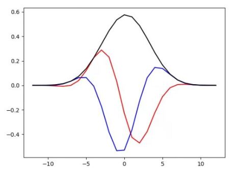
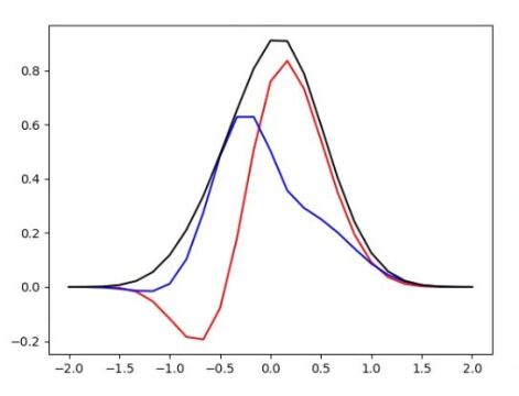
In Figure 5 and Figure 6, the red is real, the blue imaginary, and the black is the magnitude. Clearly, as time moves on, the probability amplitude of our scalar particle moves towards the attractive coulomb well. We can be more sure we are performing this simulation correctly by taking an inverse Fourier transform of the complex-valued propagator and probing it for spikes in . The author believes that these spikes would correspond to bound or resonant states of the above system.
5.3. Discussion
The above interactions are obtained by considering different, non-geometric terms in our action. It is difficult to obtain physically interesting interaction terms from purely geometric quantities; this is one of the promising features of String and M-Theory [19]. In these theories, we consider sheets and membranes rather than paths, and the quantities of interest are discrete sheet-indexed sums of phases. Like in our above work, these phases are determined by the area of the sheets, and interactions are directly built into high-genus sheets. There are a number of technical hurdles with using our above scheme to find a Membrane Theory. The first is that our input and output states are no longer points with finite degrees of freedom; string and membrane initial and final states have infinitely many degrees of freedom. The author has already obtained some results for discrete string propagators when the degrees of freedom are limited by allowing world-sheets (the sheets traced out by strings in String Theory [19]) to only be rectangular. Another means of solving this problem would be to treat the Membrane propagators as a function between sequences, where a sequence would encode uniquely the moments of a string or membrane. In either case, the work of Cano and Diaz [2] must be generalized to obtain Membrane Theory’s version of . It is not so easily seen that the space of directed sheets has some sensible expression for its volume; this would be necessary to move from discrete string propagators (of which the author has already performed some computation) to the continuous case.
6. Definitional Proofs
This section includes longer and more difficult proofs of concepts required throughout this work. Some concepts are results in themselves, and therefore ought not to be relegated to an appendix.
Theorem 8.
Let such that
where denotes some function that goes to zero as . An alternative approximation is the following
relating the continuum multinomial to Shannon entropy.
Theorem 9.
The continuous multinomial
is a finite and analytic function from .
Proof.
| (57) |
where counts Smirnov words with frequency vector . This vector denotes how many of each letter occurs in a Smirnov word. This coefficient has a nice generation function, and in [21] it was shown that Eq 57 without the root terms has nice analytic properties. Namely, it satisfies Equation 58.
| (58) |
We will use this to obtain an absolutely convergent multidimensional taylor series at 0 for the continuous multinomial (with an infinite radius of convergence). This will demonstrate the claim. Suppose we let denote the taylor series coefficients for the continuous multinomial; i.e. we have Equation 59.
| (59) |
We note that from the work of [21] (expressing Equation 57 sans square root as a Borel transform) that the following coefficients are immediate:
The non-mixed terms for in Equation 58 are first order; they give us a recursion relation for :
This gives us the recursion relation with the solution:
for . This has an infinite radius of convergence in its one direction. To proceed further, we acknowledge the symmetries of the function, and our differential equation gives us where is an arbitrary permutation of our indices. So, we need only solve consecutive partial recursion relations to obtain our full solution. Namely, we need a recursion relation for arbitrary terms of the form , where terms like provide boundary conditions. From Equation 58, we can list the lowest order differential operators with terms with in them
which, when applied to our taylor series, gives us terms as in Equation 60.
| (60) |
Now, to find the partial recurrence relation for , we need to combine all terms in Equation 57, which have only differential operators from . If we are missing an index, then that corresponds to an term with the decremented index itself. Each of these contributions to the differential operators will look like the expression from Equation 60. This gives us the partial recursion relation Equation 61 for , where runs over the number of indices missing from some differential term.
| (61) |
This gives us an algorithm to calculate for any index, by running through a higher order recursion relation until we hit zero in some index of , and then moving to a lower recursion relation until we reach . Our goal now is to use Equation 61 to bound the taylor terms into some absolutely convergent series as we have for when we evaluate the continuous multinomial along only a single coordinate. Rewriting Equation 61, we obtain Equation 62.
| (62) |
Now, we can use the above recursion relation to obtain bounds on the taylor series terms. We have a first bound in Equation 63.
| (63) |
Exhaustively applying our recursion relation Equation 62, we obtain Equation 64.
| (64) |
Each of these sums ends in . The fraction of can be bounded absolutely by a constant in terms of l, and we can consume each intermediate double sum by that constant as well. Let us call that constant . Then, we have a factor bounding this whole series, giving us the final bound in Equation 65.
| (65) |
So, this nice modified expression is analytic and finite at all values. The original expression for the continuous multinomial coefficient (in terms of volumes) has an extra factor of that multiplies each . It is clear from the above work that this would not affect the infinite radius of convergence, and we have demonstrated the well-definedness of our continuous multinomial coefficient. Since our series converges absolutely, the other expression for the multinomial (in Equation 11) may be a permutation of the series obtained above. It will converge to the same value because of our absolute convergence, and we can alternatively adopt either expression. It shall be important to adopt the more geometric expression in the coming proof.
∎
Theorem 10.
The Continuous Multinomial is a Limit of the Discrete One
Let . Then we have
This will also prove other forms of convergence (here we normalize by the maxima, we could also normalize by the integral of each expression).
Proof.
Consider the polyhedron used in the expression in Equation 11. As a polyhedron, it lies in the intersection of Lebesgue and Reimmanian measurable sets, so we have Equation 66.
| (66) |
The fact that is an dimensional polyhedron, where n refers to the number of steps allowed in a directed path, is a fact made apparent by [21]. We will just use it here. Let . We note that the multinomial function is well known to be equal to the number of monotonic paths with steps among from zero to . Therefore, we would have Equation 67
| (67) |
| (68) |
This becomes Equation 69.
| (69) |
Now, we want to introduce the fraction we have from the start of this theorem’s statement. When we do so, Equation 69 becomes Equation 70.
| (70) |
| (71) |
We apply the series transform described in Section 6 to this series; in order to reweight the series back towards less segmented paths. This gives us Equation 72.
| (72) |
∎
Theorem 11.
Let where . Then
This implies that should be some constant large number, then its Schwartz class [16], so all derivatives of it have Fourier transforms which are Schwartz class.
Proof.
Let be the taylor coefficients of the asymptotic function in Theorem 8. Then:
This is due to the fact that from [21], the paths with linear segments in the continuous multinomial correspond to taylor series coefficients with a total mixed degree of . The asymptotic function above clearly indicates where terms of fixed power in are going to be located, allowing us to properly place the powers dictated by the operator .
Splitting the factor of m and using Theorem 9 for well-behavedness to push the limit past the sum, this becomes:
This yields the theorem.
∎
Theorem 12.
Let . Then one is the set (i.e. a minimal for is this above set).
Proof.
Consider the slopes of the half-plane boundaries which form in Eq 3. The smallest magnitude slope is 1 (corresponding to ); if we had smaller slopes, would intersect non-trivially with non-local paths (a contradiction). For , there is some R sufficiently such that if , then because is the smallest slope, the equation for it must be the minimum of . So, . But, we can take any vector in and multiply its magnitude by and see that it necessarily must be parallel to . Therefore, generates all null paths. Furthermore, the arguments of Theorem 12 show that cannot be generated except by themselves and must then lie in . So, we now need only need concentrate on non-null elements in (i.e. ).
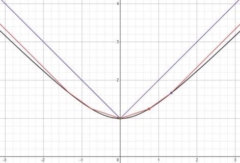
Let . This yields . If we define and , then the aforementioned set is contained within . These objects are all plotted in Figure 7. If we look at the argument of the minimum defining in Equation 3, you will see implicit equations for some lines. Namely, if we take that argument and set it equal to 1, we obtain Equation 73.
| (73) |
We introduce in Section 1 the points in as the normalized Pythagorean triples with hypotenuse less than n. If we index this set by order of their x coordinate from most to least negative, then Equation 73’s linear equations are precisely those lines adjoining to as points in . If the minimum of these lines equals 1, it implies one of these lines equals, so is composed of piecewise linear segments that adjoin and . Every point above one of these lines satisfies Equation 73 where its equal to instead of 1. This fact, along with the monotonically increasing slope between as points on , implies that between the linear segment that composes is precisely the line adjoining and . This is again illustrated in Figure 7. Since is concave up, we have .
The above fact shows us are vectors parallel to the set in the hypothesis of this Theorem. Here, we employ some facts about primitive Pythagorean triples [18]: if we divide , a Pythagorean triple, by the gcd of the three elements, then the resulting object is a primitive Pythagorean triple. These primitive pythagorean triples build up all pythagorean triples along their direction and by extension all . They also all lie in different directions, so they constitute as defined in Section 2.
∎
Theorem 13.
Let . Then where denote unit directions in
Proof.
First if then . This implies that the sum of the absolute value of the spatial coordinates equals . Therefore, it may be generated by adding elements of . This set (except in some tropical examples) lies in . Any would need to contain all of these elements as if for then and all except one is zero. So, we have obtained a minimal set required to generate null vectors. Say such that . Then and furthermore its generated by . Again, any would need to contain . So, if we show that these above vectors are the only ones upon which and agree, then we are done. We note that the surface is a polyhedral cone which touches atleast at . Let . Then, are rational points on a sphere in of radius . Meanwhile, will be a polyhedral shape with maximum distance from the origin of (as the maximum distances are aligned with the axes in the sphere). It is immediate that for , and so our ’sphere’ lies above the in the upper half space at all points except . This implies, by scaling, that the only non-null point upon which the metrics agree is multiples of .
∎
Theorem 14.
Let . Let denote some axes of symmetry of . Then, we can choose our such that . This alteration will yield the same path up to our equivalence relation on , and this equivalence class representative is unique.
Proof.
Let such that there is some index where is not in . We know so by the definition of we know for . Let be defined such that for , that for , that for . We just replaced our single difference sequence element with a finite number of difference sequence elements, all of which were in . This portion of the path all lies on the same points in ; therefore, under our equivalence relation.
If we take , by a finite number of recursions of the above argument, we obtain a such that and its composed only of difference sequences among . We can proceed by induction to show this representation of the difference sequence of among . If are not equal, then they are not directed in the same direction. So, they are locally not the same piecewise linear graph. This is a contradiction. We proceed by finite induction and show that the difference sequence is the same.
∎
Theorem 15.
Denote the set of primitive pythagorean triples with hypotenuse below as . Then, , and they are equidistributed on the unit circle when ordered according to hypotenuse (as the hypotenuse goes to infinity).
Theorem 16.
The continuum multinomial has the following property
This implies that should any of the coefficients of the continuum multinomial coefficient be zero, than the function is also zero.
Proof.
The first property of the continuum multinomial is established by Theorem 10 and the proof is performed in the same manner as Theorem 11. Namely the multiplicative property described is obtained in the discrete setting, and commutes past limits to apply to the continuum multinomial. The second property is established by an explicit equation found in [2]. Cano and Diaz found that their version of the binomial coefficient has the property ; this was obtain from the explicit expression . Now our expression for the continuum multinomial coefficient only differs in that every power has a multiplicative factor placed next to it. We can rewrite Cano’s expression in terms of these powers like so:
meaning we obtain the following expression for the continuum multinomial coefficient
| (74) |
Let . In the first term of Equation 74 goes to zero unless , in which case our multplicative factor takes it to zero. In the next expression it will always be zero, and in the third portion of Equation 74 we return to the first case. So the binomial coefficient evalautes to zero when any of its coefficients do. This, along with the multiplicative properties of the continuum multinomial already established, obtains the desired result. ∎
Acknowledgement
7. Data Availibility Statement
The manuscript has no associated data.
References
- [1] Sergio Albeverio and Sonia Mazzucchi, A survey on mathematical feynman path integrals: Construction, asymptotics, applications, pp. 49–66, Birkhäuser Basel, Basel, 2009.
- [2] Leonardo Cano and Rafael Diaz, Continuous analogues for the binomial coefficients and the catalan numbers, 2016.
- [3] Parker Duncan, Rory O’Dwyer, and Eviatar B. Procaccia, An elementary proof for the double bubble problem in norm, 2020.
- [4] by same author, Discrete double bubble solution is at most ceiling of the continuous solution, 2021.
- [5] Richard Phillips Feynman, Albert R. Hibbs, and Daniel F. Styer, Quantum mechanics and path integrals, Dover Publications, 2017.
- [6] Gerald B. Folland, Real analysis: Modern tichniques and their applications, Wiler-Interscience Publication, 1994.
- [7] Manuel Friedrich, Wojciech Górny, and Ulisse Stefanelli, The double-bubble problem on the square lattice, 2021.
- [8] James Glimm and Arthur Jaffe, Quantum physics: A functional integral point of view, Springer, 1987.
- [9] Zhang Hong-Hao, Feng Kai-Xi, Qiu Si-Wei, Zhao An, and Li Xue-Song, On analytic formulas of feynman propagators in position space, Chinese Physics C 34 (2010), no. 10, 1576–1582.
- [10] Iosif Pinelis (https://mathoverflow.net/users/36721/iosif pinelis), Asymptotics of multinomial coefficients, MathOverflow, URL:https://mathoverflow.net/q/344669 (version: 2022-01-02).
- [11] Nam-Gyu Kang and Nikolai Makarov, Gaussian free field and conformal field theory, 2011.
- [12] Mathieu Lewin, Coulomb and riesz gases: The known and the unknown, Journal of Mathematical Physics 63 (2022), no. 6, 061101.
- [13] A. Linde, Particle physics and inflationary cosmology, CRC Press, 2017.
- [14] Ralph Morrison, Tropical geometry, 2019.
- [15] Michael Edward Peskin and Daniel V. Schroeder, An Introduction to Quantum Field Theory, Westview Press, 1995, Reading, USA: Addison-Wesley (1995) 842 p.
- [16] Micheal Reed, Methods of modern mathematical physics, Academic Press, 1972.
- [17] Ramin Takloo-Bighash, A pythagorean introduction to number theory: Right triangles, sums of squares, and arithmetic, pp. 3–12, Springer International Publishing, Cham, 2018.
- [18] Lin Tan, The group of rational points on the unit circle, Mathematics Magazine 69 (1996), no. 3, 163–171.
- [19] Cumrun Vafa, The string landscape and the swampland, 2005.
- [20] Juan Pablo Vigneaux, A homological characterization of generalized multinomial coefficients related to the entropic chain rule, 2020.
- [21] T. Wakhare, C. Vignat, Q. N. Le, and S. Robins, A continuous analogue of lattice path enumeration, 2017.
- [22] Barton Zwiebach, A first course in string theory, Cambridge University Press, 2004.