FedGKD: Unleashing the Power of Collaboration in Federated Graph Neural Networks

Abstract.

Federated training of Graph Neural Networks (GNN) has become popular in recent years due to its ability to perform graph-related tasks under data isolation scenarios while preserving data privacy. However, graph heterogeneity issues in federated GNN systems continue to pose challenges. Existing frameworks address the problem by representing local tasks using different statistics and relating them through a simple aggregation mechanism. However, these approaches suffer from limited efficiency from two aspects: low quality of task-relatedness quantification and inefficacy of exploiting the collaboration structure. To address these issues, we propose FedGKD, a novel federated GNN framework that utilizes a novel client-side graph dataset distillation method to extract task features that better describe task-relatedness, and introduces a novel server-side aggregation mechanism that is aware of the global collaboration structure. We conduct extensive experiments on six real-world datasets of different scales, demonstrating our framework’s outperformance.

1. Introduction

Federated training of Graph Neural Networks (GNN) has gained considerable attention in recent years due to its ability to apply a widely used privacy-preserving framework called Federated Learning (FL) (McMahan et al., 2017; Kairouz et al., 2021) to GNN training. This approach facilitates collaborative training among isolated datasets while preserving data privacy. The protocol generally follows a typical federated learning approach, whereby the server broadcasts a global GNN model to each client. Upon receiving the model, each client trains the model using its local graph and transmits its local model to the server, which then aggregates the local weights to obtain a new global model and initiates another round of the broadcast-training-aggregation procedure. Throughout the process, the client-side graphs are kept locally, thus safeguarding privacy. Federated GNNs have successfully addressed the challenge of isolating graph data in real-life scenarios where organizations and corporations collect their private graphs, restricting others from accessing them while seeking a collaborative training approach to improve their personalized model performance.

However, the effectiveness of federated GNN frameworks is limited by graph heterogeneity issues. The isolated graph datasets exhibit significant variation, and thus, simple aggregation of all local models leads to a degradation of model performance (Ramezani et al., 2021). The recent developments of personalized federated learning (PFL) (Smith et al., 2017; Arivazhagan et al., 2019; Xu et al., 2023; Bao et al., 2023) have explored mechanisms that adapt to client heterogeneity by allowing each client to train their personalized model while encouraging inter-client collaboration through properly handling the collaboration structure among clients.

Although the PFL framework is effective in mitigating statistical heterogeneity issues, it is noteworthy that graph heterogeneity issues are more severe than that in the independent setting. This is primarily due to the complex nature of graphs that incorporate topology information. In particular, graph heterogeneity encompasses not only the distributional discrepancy of node features but also the presence of disparate graph structures (Ramezani et al., 2021). To address this challenge, a range of graph-related solutions have been proposed. However, the existing solutions for graph heterogeneity issues suffer from limited efficiency due to two reasons:

Quality of task-relatedness quantification: It has been shown in recent studies (Bao et al., 2023; Zhao et al., 2023) that high-quality characterizations of the collaboration structure among clients are crucial for the generalization performance in PFL. Existing works on PFL over graphs rely on weights and gradients (Xie et al., 2021) or graph embeddings with random input graphs (Baek et al., 2022). The former involves similarity computation of high-dimensional random vectors, which may be imprecise due to the curse of dimensionality (Hastie et al., 2009), while the latter one discards information related to local labels and losses expressivity.

Efficacy of exploiting collaboration structure: Another reason for unsatisfactory efficiency is the inadequate handling of the collaboration structure, which is typically reflected in the personalized aggregation mechanisms. Previous works base their aggregation procedures on pairwise relationships among client tasks (Baek et al., 2022), which only exploit inter-client task relatedness locally. It is therefore of interest to explore mechanisms that operate from a global point of view in a principled way.

To address the problems, we propose a novel Federated Graph Neural Network with Kernelized aggregation of Distilled information (FedGKD) that achieves better utilization of the collaboration among clients. This framework comprises two modules: A task feature extractor that utilizes a novel graph data distillation method and a task relator that aggregates local models through a mechanism that is aware of the global property of the collaboration structure inferred from the outputs of the task feature extractor. Specifically, the task feature extractor devises a novel dynamic graph dataset distillation mechanism that represents each local task by distilling local graph datasets into size-controlled synthetic graphs at every training round, enabling efficient similarity computation between clients while sufficiently incorporating local task information. The task relator first constructs a collaboration network from the distilled task features and relates tasks through a novel aggregation mechanism based on the network’s global connectivity, which measures the task-relatedness in a global sense. As a summary, our contributions are:

• We propose a task feature extractor based on a novel dynamic graph data distillation method, representing each local task with a distilled synthetic graph generated from all the local model weights trained at each round. The task features extracted from distilled graphs contain both data and model information, while also allowing for efficient evaluation of task-relatedness.

• We propose a task relator that constructs a collaboration network from the distilled graphs and relates tasks by operating a novel kernelized attentive aggregation mechanism upon local weights that encodes the global connectivity of the collaboration network.

• We conduct extensive experiments to validate that our framework consistently outperforms state-of-the-art personalized GNN frameworks on six real-world datasets of varying scales under both overlapping and non-overlapping settings.

The paper proceeds as follows. In Section 2, we present a review of related works. This is followed by the introduction of the preliminaries on GNN and FL in Section 3. Next, in Section 4, we introduce and formulate the problem of federated GNN. The detailed design of the framework to solve this problem is presented in Section 5. In Section 6, we present the experimental results. Finally, Section 7 concludes the paper.

2. Related Work

2.1. Personalized Federated Learning

The learning procedures of homogeneous federated learning (McMahan et al., 2017; Kairouz et al., 2021) are often considered as special forms of distributed optimization algorithms like local SGD (Woodworth et al., 2020). However, these methods have been shown to suffer from client heterogeneity in terms of both convergence (Karimireddy et al., 2020) and client-side generalization (Chen et al., 2021; Zhao et al., 2023). Personalized federated learning approaches have primarily focused on addressing the latter issue by incorporating adaptation strategies that can be deployed at the client side, server side, or both. Client-side adaptation methods typically utilize parameter decoupling paradigms that enable flexible aggregation of partial parameters (Arivazhagan et al., 2019; Pillutla et al., 2022) or control the optimization of local objectives by regularizing towards the global optimum (Li et al., 2021). However, these methods often overlook the overall collaboration structure among the clients (Bao et al., 2023; Zhao et al., 2023). It has been shown that with a correctly-informed collaboration structure that precisely describes the task-relatedness between clients, simple procedures can achieve minimax optimal performance (Zhao et al., 2023). On the other hand, server-side adaptation methods aim to measure the task-relatedness among clients and derive refined aggregation mechanisms. (Bao et al., 2023) utilize tools from transfer learning theory to conduct an estimating procedure that clusters clients into subgroups. (Ye et al., 2023; Xu et al., 2023) propose to optimize collaboration among clients on-the-fly by solving a quadratic program at the server-side during each aggregation step. It is important to note that server-side adaptation methods often involve the transmission of additional information other than the model parameters.

2.2. Federated Graph Representation Learning

In (Ramezani et al., 2021), the authors showed that naively applying FedAvg to distributed GNN training will result in irreducible error under distinct client-side graph structures, which hampers convergence. A recent line of work has been attempting to adopt personalization strategies for federated learning of graph neural networks. For instance, (Tan et al., 2023) uses client-side adaptation by sharing only a sub-structure of the client-side GNN. (Zhang et al., 2021) equips each client with an auxiliary neighborhood generation task. (Xie et al., 2021) applies a server-side adaptation strategy that dynamically clusters clients using intermediate gradient updates. Moreover, (Baek et al., 2022) combines client-side and server-side adaptation methods and measures task similarity using GNN outputs based on a common input random graph.

2.3. Dataset Distillation

The method of dataset distillation (Wang et al., 2018) was originally proposed as a way to improve training efficiency by distilling a large dataset into a significantly smaller one while keeping model performance almost intact. Later developments generalized the approach to graph-structured data (Jin et al., 2022b, a). A notable property of dataset distillation is that the distilled datasets are observed to exhibit good privacy protection against empirically constructed adversaries (Dong et al., 2022). This empirical property has also lead to innovations in one-shot federated learning (Zhou et al., 2020), which is very different from the setups in PFL and is considered an orthogonal application.

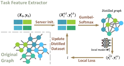
(a)

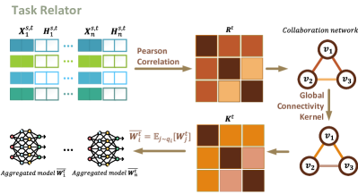
(b)

Figure 1. Overview of two modules in the proposed FedGKD framework.

3. Preliminaries

In this section, we provide a brief introduction to two key concepts in our paper: Graph Neural Network and Federated Learning, which are presented in separate subsections.

3.1. Graph Neural Network

Consider a graph $G=(V,E)$, where $V$ represents the node set and $E$ represents the edge set. The graph is associated with a node feature matrix $\mathbf{X}\in\mathbb{R}^{|V|\times D}$. We can use Graph Neural Networks (GNN) to embed nodes in the graph with low dimensional vectors. An $L$-layer GNN in the message passing form (Gilmer et al., 2017; Xu et al., 2018) is recursively defined in (1), where $\mathbf{h}_{u}^{l}$ represents the embedding of node $u$ output from the $l-$th GNN layer, $UPD$ is a function that generates embeddings based on the former layer outputs, $AGGR$ is a function that aggregates the embeddings together and $\mathcal{N}(u)$ represents the set of neighboring nodes of node $u$.

(1) $$\mathbf{h}_{u}^{l}=UPD^{l}[\mathbf{h}_{u}^{l-1},AGG^{l}(\{\mathbf{h}_{v}^{l-1}:v\in\mathcal{N}(u)\})].$$

In general, the outputs of $L-$th GNN layers are passed through a customized READOUT layer to accomplish various graph-related tasks. For instance, in node classification tasks, a simple READOUT layer can be selected as a linear layer with the number of categories as the output dimension.

3.2. Federated Learning

Federated Learning (FL) was introduced to address data isolation issues while preserving privacy (McMahan et al., 2017). It enables collaborative training among clients without exposing raw datasets. A typical FL framework consists of three stages: (1) model initialization, where the server broadcasts initial model weights to all clients; (2) local training, where each client trains a local model using the initial model weights and its own dataset, and uploads the local model to the server; (3) global aggregation, wherein the server aggregates the local models into one or more new models and broadcasts the result to each client to initiate the next training round. The FL procedure typically alternates between stage (2) and (3) until convergence.

4. Problem Formulation

A personalized federated GNN framework aims to collaboratively learn local GNN models in a privacy-preserving manner. This allows the local models to fit their respective local datasets while leveraging information from other clients to improve sample efficiency. In the system, there are $n$ clients and one server. Each client stores a local graph dataset $G_{i}=(V_{i},E_{i},\mathbf{X}_{i})$, where $V_{i}$ represents the node set, $E_{i}$ represents the edge set, $\mathbf{X}_{i}\in\mathbb{R}^{|V_{i}|\times D}$ contains the node features, and $[n]$ denotes the set of positive integers from $1$ to $n$. Within the system, the $n$ clients train $n$ GNN models $f(G_{i};\mathbf{W}_{i}),i\in[n]$, with the same structure but different parameters ${\mathbf{W}i},{i\in[n]}$. Additionally, we assume that the prediction function $f=g\circ h$ is composed of an $L$-layer message passing GNN module $h$ with a hidden dimension of $d$, and a READOUT module $g$ that maps the node embedding extracted by $h$ to downstream task predictions. The goal of a personalized federated GNN framework is formulated as

(2) $$\min_{\mathbf{W}_{i}\in\Omega_{i},i\in[n]}\sum_{i=1}^{n}\mathcal{L}(f(G_{i};\mathbf{W}_{i}),\mathbf{y}_{i})$$

where $\mathcal{L}$ is the loss function, and $\mathbf{y}_{i}$ contains all the labels belonging to client $i$. To encourage collaboration among clients, the parameter spaces $\Omega_{i},i\in[n]$, are usually assumed to be related (Duan and Wang, 2022). The precise structure of this relation is sometimes implicit and instead reflected in the optimization procedure (Chen et al., 2022a). Under the graph representation learning setup, we require $\Omega_{i}$ to capture the relatedness between corresponding tasks, taking into account the topological structure of the graph (Girvan and Newman, 2002), as well as feature and label information. Additionally, we impose an extra constraint to ensure that local models do not deviate significantly from each other. This is achieved by adding a proximal regularization term that prevents overfitting to local data, which has been shown to benefit many federated learning procedures (Li et al., 2020, 2021).

5. Design

5.1. Overview

In this section, we provide a detailed introduction to our personalized federated graph learning framework, which aims to address two major problems:

• How to extract task features from the local dataset $G_{i}$ and local model parameters $\mathbf{W}_{i}$?

• How to relate local tasks with each other using the task features to aggregate $\mathbf{W}_{i}$?

To address the first question, we propose a feature extractor based on dataset distillation, as illustrated in Fig. LABEL:fig:tfe, that captures all the information within the local model. The feature extractor generates a small graph in each round based on the current local model weights. To mitigate graph heterogeneity, the server distributes a common initial graph to all clients, preventing significant deviations among the distilled graphs.

To address the second question, we draw insights from recent advancements in kernel formulations of self-attention (Tsai et al., 2019; Chen et al., 2022b). We view the personalized aggregation process as an attentive mechanism operating on the collaboration network among clients. We observe that several contemporary aggregation schemes overlook the global task relatedness. Leveraging tools from kernel theory, we derive a refined aggregation scheme based on exponential kernel construction that effectively incorporates global information, as shown in Fig. LABEL:fig:tr.

5.2. Task Feature Extractor

5.2.1. Motivation

It is well known in the theory of multi-task learning (Hanneke and Kpotufe, 2022; Duan and Wang, 2022) that correct specifications of task relatedness may fundamentally impact the model performance, which has also been recently discovered in PFL (Zhao et al., 2023). In hindsight, the ideal characterization of a (local) graph representation learning task might be either the joint distribution of the local graph, feature and label variables; or the Bayes optimal learner dervied from the joint distribution (Zhao et al., 2023). However, none of this information are available during FL, and various surrogates have been proposed in the context of graph PFL that extracts task features from the (local) empirical distribution and the learned model.

The most ad-hoc solution is to use weights (Long et al., 2023; Ye et al., 2023) and gradients (Sattler et al., 2020), which are typically high-dimensional (random) vectors. However, computing their relations using metrics like Euclidean or cosine similarity can be unreliable due to the curse of dimensionality phenomenon (Hastie et al., 2009), as empirically validated in (Baek et al., 2022). As a notable state-of-the-art model, FedPUB (Baek et al., 2022) uses low-dimensional graph embeddings that are produced by passing a shared random graph between clients. However, since the embedding computation only involves message passing GNN layers, the resulting embeddings are incomplete, as they fail to represent the READOUT layer that follows these GNN layers. The READOUT layer encodes label-related information. This limitation is significant when two datasets share similar graph distributions but have divergent label distributions. This can result in two local models with similar GNN layer weights but different READOUT layer weights. In such cases, the embeddings, which are outputs of similar GNN layers, cannot distinguish between the two datasets. We conducted a small experiment to validate this point. We visualized the embeddings for GCN layers trained on two datasets with similar graph distributions but divergent label distributions in Fig. 2. To be more specific, we trained node embeddings on the original Cora graph (Yang et al., 2016) and a revised Cora graph in which the label $y_{v}\in[C]$ of any node $v$ is modified to $C+1-y_{v}$, where $C=7$ is the number of classes in Cora. The results show that the two embedding spaces are similar, as vertices belonging to the same community are located in similar positions in the space, as shown in Fig. 2.

To address the challenges encountered in PFL frameworks, we leverage graph dataset distillation, a method that simultaneously compresses the local data distribution and the learned local model into a size-controlled small dataset that is comparable across all client tasks. In the following sections, we will introduce dataset distillation and explain how we incorporate it into our framework.

5.2.2. Dataset Distillation

Dataset distillation (Wang et al., 2018) (DD) is a centralized knowledge distillation method that aims to distill large datasets into smaller ones. For client $i$, a distilled dataset $(G_{i}^{s},\mathbf{y}_{i}^{s})$ is defined such that a neural network model trained on $G_{i}^{s}$ can achieve comparable performance to the one trained on the original dataset $G_{i}$, as formulated in (3).

(3) $$\min_{G_{i}^{s},\mathbf{y}_{i}^{s}}\mathcal{L}(f(G_{i};\mathbf{W}_{i}^{s}),\mathbf{y}_{i})\quad\text{s.t. }\mathbf{W}_{i}^{s}=\min_{\mathbf{W}_{i}^{\prime}}\mathcal{L}(f(G_{i}^{s};\mathbf{W}_{i}^{\prime}),\mathbf{y}_{i}^{s})$$

According to previous studies (Jin et al., 2022b), many datasets can be distilled into condensed ones with sizes that are only around $1\%$ of the original dataset while still preserving model performance. Moreover, it has been empirically reported that distilled datasets offer good privacy protection (Dong et al., 2022).

Based on this observation, we propose using statistics of the distilled local datasets as features that describe local tasks and obtain task-relatedness by evaluating the similarities between distilled dataset characteristics. As a straightforward adaptation of vanilla DD to federated settings, we may conduct isolated distillation steps before the federated training and fix the estimated task-relatedness during federated training. This strategy could be implemented using off-the-shelf DD algorithms on graphs (Jin et al., 2022b, a). However, the quality of the distilled local datasets may be affected by (local) sample quality and quantity. Since PFL approaches typically improve local performance, we propose a refinement of the aforementioned static distillation strategy that allows clients to distill their local datasets during the federated training process, resulting in a series of distilled datasets ${G_{i}^{s,t},\mathbf{y}_{i}^{s,t}}{t\in[T]}$ for each client $i$, with its corresponding distillation objective at round $t$ being:

(4) $$\min_{G_{i}^{s,t},\mathbf{y}_{i}^{s,t}}\mathcal{L}(f(G_{i}^{s,t};\mathbf{W}_{i}^{t}),\mathbf{y}_{i}^{s,t}).$$

Apart from its capability to adapt to the federated learning procedure, the objective (4) is computationally more efficient than the vanilla DD objective (3) as it avoids the bi-level optimization problem, which is difficult to solve (Wang et al., 2018). Instead, the objective (4) leverages the strength of the federated learning process, which usually produces performative intermediate results after a few rounds of aggregations. We refer to (4) as a dynamic distillation strategy. Next, we present a detailed implementation of the proposed dynamic distillation procedure.

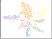
(a)

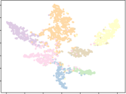
(b)

Figure 2. Embedding spaces (depicted using two leading principle components) trained on two same graphs with divergent labels: vertices belonging to the same community have the same color.

5.2.3. Implementation

There are two algorithmic goals regarding the implementation of (4): Firstly, the distilled datasets should allow efficient similarity comparisons. Secondly, the problem should be efficiently solved so that the extra computation cost for each client is controllable. Note that both goals are non-trivial since the optimization involves a graph-structured object that is not affected by permutations, resulting in alignment issues when performing similarity computation. The solution is detailed in Algorithm 2 in Appendix A. Specifically, at each round $t\in[T]$, the size of the distilled graph across all clients will be fixed at $m\times C$, where $m$ represents the number of representative nodes in each category. The server first initializes node features $\mathbf{X}_{0}$, with each entry drawn independently from a standard Gaussian distribution $\mathcal{N}(0,1)$. The initial labels $\mathbf{y}_{0}$ are set to ensure that there are $m$ nodes belonging to each category. The tuple $(\mathbf{X}_{0},\mathbf{y}_{0})$ is broadcast to each client as the initial value of their local objectives, while the construction of the distilled graph structure is left to the clients’ side to reduce communication cost. This common initialization technique alleviates the alignment issue between distilled graphs.

After each client receives the initial features $\mathbf{X}_{0}$ and labels $\mathbf{y}_{0}$, it begins to update the features and labels. Since directly optimizing the graph structure (i.e., among the space of possible binary matrices) is computationally intractable, we use the following simple generative model that describes the relationship between node features and edge adjacency for the distilled graph: For a pair of nodes (regarding the distilled graph) $u$ and $v$ with features $\mathbf{x}_{u}^{s}$ and $\mathbf{x}_{v}^{s}$, the probability of them being adjacent is given by

(5) $$\mathbb{P}[\mathbf{A}^{s}_{uv}=1]=\dfrac{e^{\langle\mathbf{x}^{s}_{u},\mathbf{x}^{s}_{v}\rangle-\gamma}}{1+e^{\langle\mathbf{x}^{s}_{u},\mathbf{x}^{s}_{v}\rangle-\gamma}},$$

where $\gamma>0$ is a hyperparameter that controls edge sparsity. Construction of the distilled graph involves sampling from the above distribution, which is not differentiable. Hence we adopt the Gumbel-softmax mechanism (Jang et al., 2016; Maddison et al., 2016) to generate approximate yet differentiable samples. In particular, for each $u,v$, we first draw two independent samples $\omega$ and $\omega’$ from the standard Gumbel distribution. Next, we compute the following approximation:

(6) $$p_{uv}(\tau_{g})=\dfrac{e^{\left(\langle\mathbf{x}^{s}_{u},\mathbf{x}^{s}_{v}\rangle-\gamma+\omega-\omega^{\prime}\right)/\tau_{g}}}{1+e^{\left(\langle\mathbf{x}^{s}_{u},\mathbf{x}^{s}_{v}\rangle-\gamma+\omega-\omega^{\prime}\right)/\tau_{g}}},$$

which adopts a distribution limit $\lim_{\tau_{g}\rightarrow 0}p_{uv}(\tau_{g})\overset{d}{=}\mathbf{A}^{s}_{uv}$. In practice, we use the straight-through trick (Jang et al., 2016) to obtain discrete samples from (6) while allowing smooth differentiation. We denote the distilled graph as $G^{s}=(\mathbf{X}^{s},\mathbf{P})$ with $\mathbf{P}$ being the (approximated) adjacency matrix, with each entry derived from (6).

We utilize the local model weights to assess how well the distilled dataset fits the model and update $\mathbf{X}^{s}$ and $\mathbf{y}^{s}$ based on the same classification loss as each client’s local learning objective. In practice, we have found that a few steps of gradient updates suffice for the learning performance. After obtaining the distilled graph, we extract task features ${M_{i}^{t}}_{i\in V_{c}}$ for client $i$ at round $t$ as follows:

(7) $$\mathbf{M}^{t}_{i}=\left[\mathbf{X}^{s,t}_{i}\operatorname*{\mathchoice{\Big{\|}}{\big{\|}}{\|}{\|}}\mathbf{H}^{s,t}_{i}\right],\quad\mathbf{H}^{s,t}_{i}:=h(\mathbf{G}^{s,t}_{i},\mathbf{W}^{t}_{i}).$$

Note that although the distilled labels are not included in the task feature, the label information is fused into $\mathbf{X}^{s}$ during the distillation process. We will present an empirical study regarding other potential choices of task feature maps in section 6.2.7.

5.3. Task relator

5.3.1. Motivation

We represent the estimated relationship among tasks using a time-varying collaboration network $G_{c}^{t}=(V_{c},\mathbf{R}^{t})$, where $t\in[T]$, $V_{c}=[n]$, and $\mathbf{R}^{t}\in\mathbb{R}^{n\times n}$ represents the time-dependent task relation matrix. The entry $r^{t}_{ij}$ measures the task-relatedness between client $i$ and client $j$, obtained by computing similarities of their corresponding task features $\mathbf{M}^{t}_{i}$ and $\mathbf{M}^{t}_{j}$. This idea has been adopted in some recent PFL proposals (Chen et al., 2022a; Ye et al., 2023).

Since the matrix $\mathbf{R}^{t}$ encodes pairwise relationships among client tasks, it offers great flexibility in defining personalized aggregation protocols. We formulate the protocols as the following expectation:

(8) $$\overline{\mathbf{W}_{i}^{t}}\leftarrow\mathbb{E}_{j\sim q_{i}}\left[\mathbf{W}_{j}^{t}\right]$$

where $q_{i}$ is a client-specific distribution over $[n]$, with a trivial case of uniform distribution that corresponds to the aggregation rule in FedAVG. The above formulation is closely connected to the self-attention mechanism (Vaswani et al., 2017). In particular, inspired by recent developments that generalize self-attention using kernel theory (Tsai et al., 2019), we parameterize $q_{i}$ using a kernel-induced distribution:

(9) $$q_{i}[j]=\dfrac{k(i,j)}{\sum_{j^{\prime}\in[n]}k(i,j^{\prime})},$$

where $k(\cdot,\cdot)$ is a kernel function.

The most straightforward choice would be the softmax kernel (Choromanski et al., 2020) that uses the exponentiated edge weights $k(i,j)=e^{r_{ij}}$. However, this method disregards other weights, resulting in a kernel function that only takes local connectivity in the collaboration network into account, overlooking global connectivity. We illustrate this point using the example in Fig. 3, where a collaboration network with three vertices has weighted links of $r_{12}<r_{23}=r_{13}$. If we directly use $r_{ij}$ and normalize them, the average local model weights $\overline{\mathbf{W}_{1}^{t}}$ will be very close to $\mathbf{W}_{3}^{t}$ and far from $\mathbf{W}^{t}_{2}$. However, the relation between node 1 and 2 is much stronger than what the quantity $r_{12}$ indicates, as they are also linked by another two-hop path comprising two heavily-weighted edges $(1,3)$ and $(2,3)$. A recent work (Chen et al., 2022a) attempts to capture information beyond local task pairs by incorporating a GNN-like mechanism over a sparsified collaboration network. This approach aims to integrate more information through a few rounds of message passing. While the approach in (Chen et al., 2022a) extends the scope of similarity evaluation, it still operates in a local sense due to the finiteness of message passing rounds and the inherent limitation of oversmoothing phenomenon. To address this limitation, our framework proposes a novel kernel function that incorporates all the global connectivity. Specifically, our kernel extracts connectivity at hops from 1 to infinity while favoring connectivity with fewer hops.

(a) local connectivity

(b) global connectivity

Figure 3. Comparison of local and global connectivity

5.3.2. Construction of the task relator

According to the previous discussions, implementing the task relator involves the design of two modules: A collaboration graph construction procedure based on the extracted task features $\{M_{i}^{t}\}_{i\in V_{c}}$ and a global-connectivity-aware aggregation mechanism.

Dataset	Cora			CiteSeer			PubMed
# Clients	10	30	50	10	30	50	10	30	50
Local	46.88$\pm$1.23	66.45$\pm$0.81	70.32$\pm$0.68	51.42$\pm$1.75	59.06$\pm$1.64	61.40$\pm$1.45	76.75$\pm$0.20	77.46$\pm$0.20	76.02$\pm$0.33
FedAvg	49.75$\pm$1.32	46.20$\pm$2.67	43.48$\pm$3.97	54.79$\pm$2.86	54.14$\pm$1.41	57.52$\pm$1.98	78.53$\pm$0.68	80.99$\pm$0.26	79.53$\pm$0.06
FedProx	50.79$\pm$2.00	54.72$\pm$5.21	62.11$\pm$2.02	56.31$\pm$5.81	59.41$\pm$0.68	63.29$\pm$1.21	77.32$\pm$0.88	80.99$\pm$0.51	79.60$\pm$0.21
FedPer	52.83$\pm$0.55	67.15$\pm$0.85	70.27$\pm$0.34	57.14$\pm$1.45	62.21$\pm$1.80	63.26$\pm$1.95	79.85$\pm$0.31	80.59$\pm$0.06	80.28$\pm$0.13
FedPub	52.58$\pm$1.51	67.30$\pm$0.99	42.81$\pm$5.70	56.06$\pm$2.29	62.12$\pm$0.49	64.18$\pm$1.88	79.70$\pm$0.21	80.97$\pm$0.22	80.56$\pm$0.23
FedSage	49.25$\pm$0.50	59.42$\pm$1.03	59.99$\pm$0.23	55.54$\pm$6.95	55.63$\pm$7.00	62.73$\pm$1.09	77.87$\pm$0.50	80.97$\pm$0.24	79.36$\pm$0.73
GCFL	49.52$\pm$0.33	46.78$\pm$4.32	45.55$\pm$6.03	56.03$\pm$2.04	53.91$\pm$0.38	56.43$\pm$0.41	76.03$\pm$2.04	79.58$\pm$0.13	78.68$\pm$0.15
FedStar	43.09$\pm$0.72	61.60$\pm$0.30	67.77$\pm$1.25	46.45$\pm$0.17	54.78$\pm$2.12	58.96$\pm$1.81	75.45$\pm$0.14	76.45$\pm$0.43	74.71$\pm$0.52
Ours	53.26$\pm$1.42	67.88$\pm$1.09	70.41$\pm$0.51	58.19$\pm$1.82	62.30$\pm$1.33	64.58$\pm$0.55	79.90$\pm$0.53	81.65$\pm$0.34	80.82$\pm$0.20
Dataset	Amazon Photo			Amazon Computers			Ogbn Arxiv
# Clients	10	30	50	10	30	50	10	30	50
Local	46.57$\pm$0.15	69.25$\pm$0.25	79.42$\pm$0.34	51.82$\pm$0.62	65.69$\pm$0.94	68.57$\pm$0.35	34.76$\pm$0.50	46.98$\pm$0.18	47.45$\pm$0.19
FedAvg	43.10$\pm$2.68	44.75$\pm$4.82	46.38$\pm$1.07	44.45$\pm$0.26	52.93$\pm$1.05	53.91$\pm$0.57	41.40$\pm$0.46	44.22$\pm$0.80	43.74$\pm$2.60
FedProx	43.58$\pm$2.05	45.29$\pm$0.53	42.76$\pm$5.23	42.59$\pm$4.17	53.58$\pm$1.56	53.91$\pm$0.57	41.35$\pm$0.20	44.68$\pm$0.62	47.02$\pm$0.52
FedPer	52.20$\pm$0.99	71.76$\pm$0.57	81.65$\pm$0.06	55.04$\pm$0.33	67.55$\pm$1.42	68.79$\pm$0.51	38.77$\pm$0.44	47.46$\pm$0.18	50.51$\pm$0.15
FedPub	45.69$\pm$2.10	64.50$\pm$0.48	76.58$\pm$0.85	50.15$\pm$1.57	60.81$\pm$0.52	63.82$\pm$0.62	42.18$\pm$0.36	50.58$\pm$0.21	51.11$\pm$0.56
FedSage	47.79$\pm$0.76	58.26$\pm$2.35	58.99$\pm$1.58	47.98$\pm$0.84	56.82$\pm$0.43	63.13$\pm$0.86	42.18$\pm$0.11	45.43$\pm$0.40	46.08$\pm$0.27
GCFL	46.93$\pm$0.55	48.95$\pm$0.48	40.76$\pm$8.08	56.02$\pm$1.04	58.38$\pm$2.16	52.97$\pm$1.74	41.32$\pm$0.23	46.26$\pm$1.12	46.16$\pm$0.34
FedStar	39.05$\pm$0.43	64.51$\pm$0.28	77.35$\pm$0.69	47.93$\pm$0.82	61.67$\pm$1.01	64.34$\pm$0.71	40.92$\pm$0.13	44.28$\pm$0.19	45.27$\pm$0.35
Ours	56.07$\pm$1.44	72.15$\pm$0.49	81.91$\pm$0.29	56.56$\pm$0.15	68.43$\pm$0.28	69.11$\pm$1.07	43.02$\pm$0.04	48.32$\pm$0.14	52.38$\pm$0.12

Table 1. Node classification performance (%) on overlapping datasets

Dataset	Cora			CiteSeer			PubMed
# Clients	5	10	20	5	10	20	5	10	20
Local	80.44$\pm$1.77	79.58$\pm$1.07	79.46$\pm$0.51	71.28$\pm$1.32	68.93$\pm$0.79	70.49$\pm$0.88	84.98$\pm$0.67	83.34$\pm$0.42	82.92$\pm$0.41
FedAvg	72.91$\pm$6.59	69.23$\pm$1.03	47.79$\pm$2.61	72.43$\pm$0.99	70.33$\pm$1.37	67.18$\pm$1.17	82.02$\pm$0.15	83.17$\pm$1.35	76.50$\pm$0.20
FedProx	63.96$\pm$3.07	71.39$\pm$4.16	70.88$\pm$5.90	73.63$\pm$0.85	42.86$\pm$2.59	42.31$\pm$3.18	83.99$\pm$0.17	83.57$\pm$0.09	83.93$\pm$0.89
FedPer	81.37$\pm$1.58	76.73$\pm$0.95	77.24$\pm$1.62	70.45$\pm$2.00	67.14$\pm$6.95	71.13$\pm$0.76	85.59$\pm$0.18	85.42$\pm$0.12	83.75$\pm$0.14
FedPub	82.33$\pm$1.46	78.27$\pm$1.46	79.15$\pm$1.08	74.11$\pm$1.58	72.12$\pm$1.83	68.16$\pm$1.41	86.22$\pm$0.21	85.58$\pm$0.31	84.79$\pm$0.46
FedSage	72.07$\pm$0.36	69.66$\pm$0.27	59.28$\pm$0.38	70.64$\pm$3.04	65.54$\pm$6.95	63.02$\pm$1.49	84.64$\pm$0.60	83.39$\pm$1.29	84.92$\pm$0.45
GCFL	79.91$\pm$1.93	73.25$\pm$4.39	76.37$\pm$1.82	71.37$\pm$2.54	67.58$\pm$0.61	63.54$\pm$3.34	84.24$\pm$0.57	83.47$\pm$0.29	83.72$\pm$0.47
FedStar	79.33$\pm$0.69	78.26$\pm$0.22	80.40$\pm$0.30	69.47$\pm$1.77	70.25$\pm$1.26	68.50$\pm$0.68	81.96$\pm$0.96	81.39$\pm$0.17	80.15$\pm$0.66
Ours	83.37$\pm$1.59	80.06$\pm$1.27	81.17$\pm$0.63	75.25$\pm$1.38	74.18$\pm$1.14	71.17$\pm$1.69	87.05$\pm$0.19	86.53$\pm$0.73	86.38$\pm$0.30
Dataset	Amazon Photo			Amazon Computers			Ogbn Arxiv
# Clients	5	10	20	5	10	20	5	10	20
Local	77.97$\pm$0.29	86.14$\pm$1.05	86.37$\pm$0.17	65.90$\pm$0.29	74.41$\pm$1.51	81.81$\pm$0.50	56.93$\pm$0.89	56.54$\pm$0.37	57.79$\pm$0.89
FedAvg	53.49$\pm$5.87	45.82$\pm$1.88	35.15$\pm$1.03	46.03$\pm$1.93	39.04$\pm$3.68	43.74$\pm$8.15	55.84$\pm$0.88	61.02$\pm$0.32	59.30$\pm$0.18
FedProx	71.08$\pm$3.11	56.78$\pm$4.31	44.61$\pm$5.89	37.72$\pm$0.94	36.44$\pm$0.35	36.89$\pm$0.27	62.05$\pm$1.10	61.77$\pm$0.78	57.79$\pm$0.26
FedPer	68.19$\pm$1.68	77.15$\pm$0.14	78.96$\pm$0.68	64.30$\pm$0.34	64.47$\pm$0.20	70.44$\pm$0.57	61.57$\pm$0.50	61.52$\pm$0.37	62.73$\pm$0.26
FedPub	86.76$\pm$1.71	87.80$\pm$2.44	88.72$\pm$3.09	68.65$\pm$2.53	77.02$\pm$0.87	80.71$\pm$0.79	67.50$\pm$0.32	66.80$\pm$0.32	62.11$\pm$0.56
FedSage	51.28$\pm$7.30	51.68$\pm$7.28	51.39$\pm$7.22	42.88$\pm$5.23	50.41$\pm$7.84	57.06$\pm$0.42	58.63$\pm$1.29	61.65$\pm$0.45	54.86$\pm$1.77
GCFL	68.17$\pm$8.37	82.74$\pm$3.15	87.55$\pm$2.28	55.36$\pm$2.50	72.53$\pm$1.38	82.87$\pm$1.83	59.75$\pm$3.46	63.63$\pm$0.36	55.35$\pm$4.58
FedStar	85.67$\pm$0.31	86.85$\pm$0.09	87.60$\pm$0.68	71.88$\pm$1.70	78.81$\pm$1.41	83.42$\pm$0.73	58.96$\pm$0.82	60.77$\pm$0.46	61.36$\pm$0.14
Ours	89.16$\pm$0.04	88.83$\pm$0.85	89.53$\pm$0.73	72.75$\pm$2.16	82.68$\pm$0.73	84.23$\pm$0.41	68.52$\pm$0.14	67.87$\pm$0.27	65.27$\pm$0.51

Table 2. Node classification performance (%) on non-overlapping datasets

To form the collaboration graph, we use the following feature-wise average correlation as the pairwise task-relatedness:

(10) $$r_{ij}^{t}=\frac{1}{d+D}\sum_{k=1}^{d+D}\textsf{corr}\left(\mathbf{M}_{i}^{t}[:,k],\mathbf{M}_{j}^{t}[:,k]\right),$$

where corr stands for Pearson’s correlation coefficient(Lehmann and Casella, 2006). Next we discuss the construction of the global-connectivity-aware aggregation mechanism. Inspired by the property of exponential kernels (Kondor and Lafferty, 2002) that translates local structure into global ones, we use an element-wise exponentiated matrix exponential with two temperature parameters $\tau$ and $\tau_{s}$:

(11) $$k(i,j)=e^{\tau_{s}s_{ij}},\mathbf{S}=\{s_{ij}\}_{i\in V,j\in V}=e^{\tau\mathbf{R}}=\sum^{\infty}_{\kappa=1}\frac{1}{\kappa!}(\tau\mathbf{R})^{\kappa}.$$

From the right hand side of (11), we may interpret $s_{i,j}$ as encoding the relatedness of client $i$ and $j$ via conducting infinite rounds of message passing, thereby reflecting their global connectivity structure. Then, $k(i,j)$ scales the global connectivity into $\mathbb{R}^{+}$ range for further normalization into the client-specific distribution $q_{i}$ over $[n]$. The parameter $\tau$ is used to control the level of personalization, where $\tau\rightarrow 0$ indicates no personalization (FedAVG) and $\tau\rightarrow\infty$ indicates local training. The parameter $\tau_{s}$ strikes a balance between the contribution of local and global information. It is worth noting that there are other notions of global connectivity measures, such as effective resistance (Black et al., 2023), which are also applicable. However, here we stick to the matrix exponential due to its loose requirements of arbitrary local similarity $\mathbf{R}$. We will prove in appendix D that the function $k$ in (11) is a valid kernel over the domain $[n]$.

5.4. Complexity considerations

In comparison to vanilla FedAVG, the proposed framework requires additional local computations, a server-side matrix exponential operation, as well as extra communication costs. Let us briefly discuss the complexity of these procedures. Firstly, the dataset distillation procedure operates on small-scale graphs, making the total computation cost negligible compared to local training. Secondly, the matrix exponential operation upon $\mathbf{R}$ has a time complexity of $O(n^{3})$. This complexity is controllable in practice since the number of clients, $n$, is typically small or moderate. Finally, the extra communication cost per client per aggregation step depends on the formulation of the task feature map. According to (7), the extra communication cost is $O(bmC(d+D))$, where $b$ is the number of bits required to represent a floating-point number. This cost is comparable to the communication cost of a GNN. It is noteworthy that since GNN models are typically shallow, the communication cost of parameters is often dominated by the computation cost of local training. Moreover, the communication cost can be further reduced if a more compact task feature, such as the distilled graph embedding, is used. We will empirically investigate such alternatives in section 6.2.7.

6. Experiments

This section presents the empirical analysis of our framework, which includes a performance comparison, convergence analysis, and multiple ablation studies.

6.1. Experiment Setup

6.1.1. Datasets

We have tested the performance on six different graph datasets of varying scales: Cora, CiteSeer, PubMed, Amazon Computer, Amazon Photo, and Ogbn arxiv (Yang et al., 2016; Shchur et al., 2018; Hu et al., 2020). To split each graph into subgraphs, we employed the Metis graph partition algorithm following the setup in (Baek et al., 2022). Each client stores one subgraph from the original graph. We have conducted a node classification task by sampling the vertices into training, validation and testing vertices according to ratio 0.3, 0.35 and 0.35 before splitting. Appendix B.1 provides detailed descriptive statistics of the datasets.

6.1.2. Baselines

We compared our framework with eight different baselines, categorized into four types: (1) Local, which serves as the standard baseline without federated learning; (2) Two traditional FL baselines, including FedAvg (McMahan et al., 2017) and FedProx (Li et al., 2020); (3) One state-of-the-art personalized FL baseline, FedPer (Arivazhagan et al., 2019); (4) Four state-of-the-art personalized federated GNN baselines, including FedPub (Baek et al., 2022), FedSage (Zhang et al., 2021), GCFL (Xie et al., 2021), and FedStar (Tan et al., 2023). For detailed introductions of the baselines, please refer to Appendix B.2.

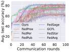
(a)

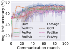
(b)

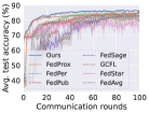
(c)

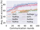
(d)

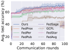
(e)

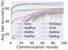
(f)

Figure 4. Convergence plot for the non-overlapping setting with 5 clients. We visualize the first 100 communication rounds.

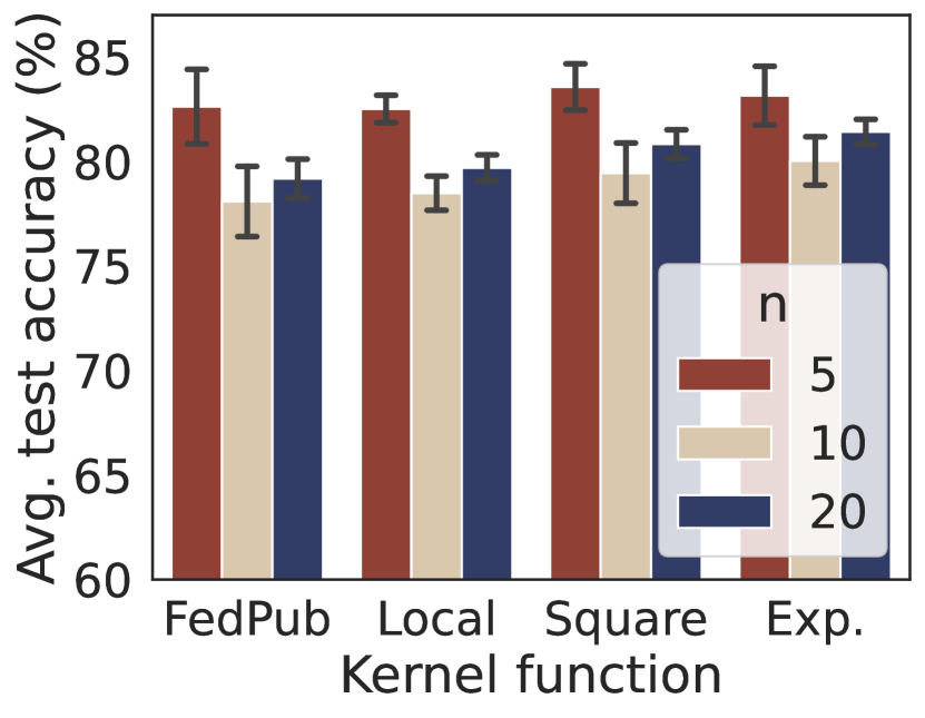
Figure 5. Effects of kernel functions

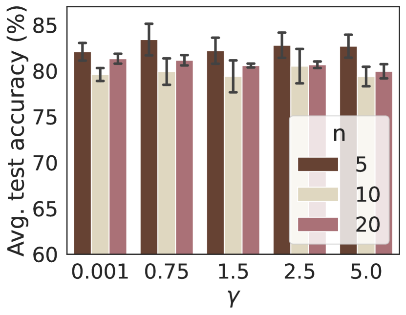
Figure 6. Effects of sparsity control coefficient $\gamma$

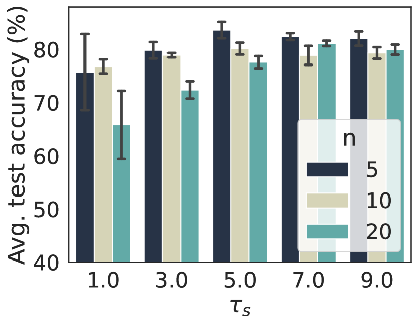
Figure 7. Effects of temperature on element-wise exponential $\tau_{s}$

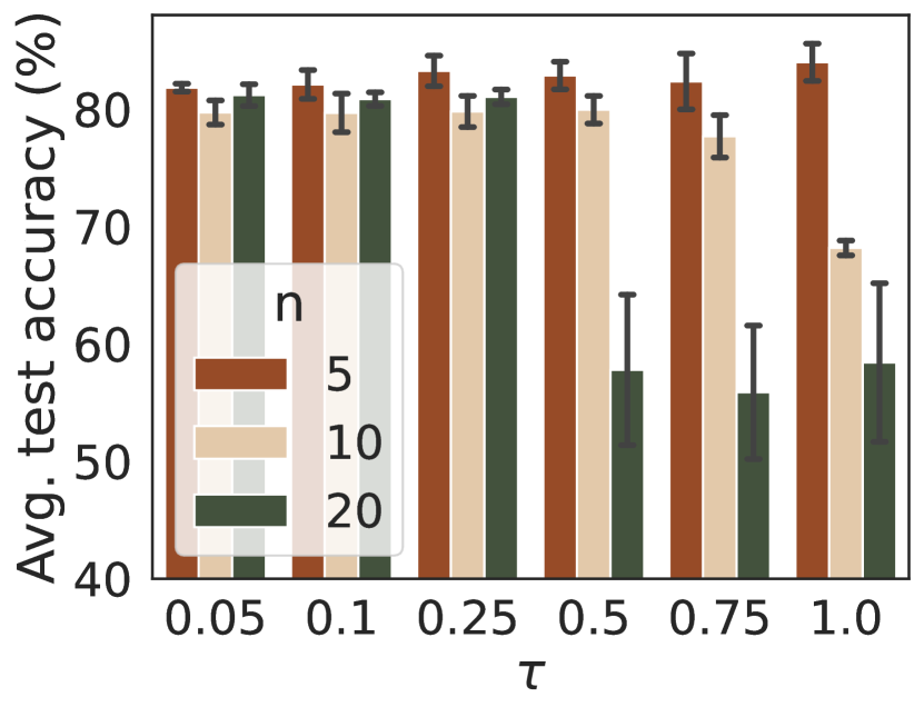
Figure 8. Effects of temperature on local connectivity matrix exponential $\tau$

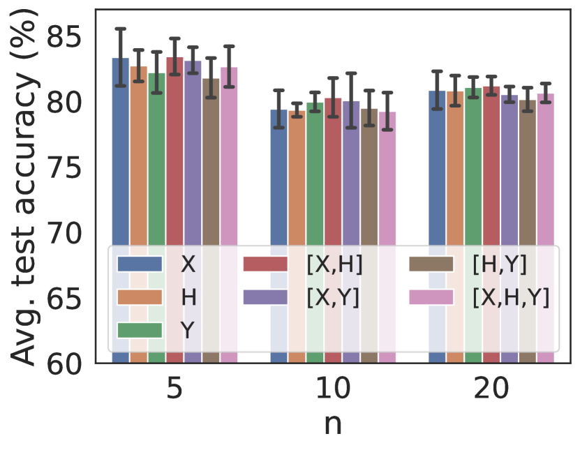
Figure 9. Effects of of task features from distilled graphs

6.1.3. Implementation Details

We utilize a two-layer GCN (Kipf and Welling, 2017) followed by a linear READOUT layer. The dimension of the embeddings is set to 128. To optimize learning, we employ the Adam optimizer with weight decay $10^{-6}$ (Kingma and Ba, 2014). The smoothing parameter $\tau_{g}$ in Gumbel-softmax is set to 1, following the technique in (Jang et al., 2016). To monitor the training progress, we use an early-stop mechanism. If the validation accuracy decreases for 20 consecutive rounds, the FL framework stops immediately. Each experiment is conducted over 3 runs with different random seeds. Implementation of all methods is done using PyTorch Geometric (Fey and Lenssen, 2019) on an NVIDIA Tesla V100 GPU. For further details, please refer to Appendix B.3.

6.2. Results

6.2.1. Performance Comparison

We evaluate the node classification performance of various frameworks using six real-world datasets of differing scales. Tables 1 and 2 present the average test accuracy and its standard deviation for overlapping and non-overlapping settings, respectively. Our framework consistently outperforms all other methods across all datasets. Traditional FL baselines, such as FedAvg and FedProx, which lack local adaptation, are consistently inferior to our Local framework in multiple scenarios. Despite using local task statistics for personalization, the feature extraction schemes of FedPer, FedStar, FedSage, and GCFL are less effective and perform worse than our framework. FedPub performs worse than our method due to the absence of information contained in local READOUT layers when describing tasks and inefficient exploitation of the global collaboration structure.

6.2.2. Convergence Analysis

Fig.4 illustrates the convergence behavior of the average test accuracy over the first 100 rounds with 5 clients in the system. It is evident that our proposed framework exhibits a rapid convergence rate towards the highest average test accuracy. This can be attributed to the framework’s ability to efficiently capture the local task features and identify pairwise relationships.

6.2.3. Effects of the proposed task relator

The primary goal of this study is to investigate the benefits of incorporating the global information. Specifically, we tested with FedGKD along with two local variants obtained via replacing the matrix $S$ in (11) on the Cora dataset. The local variant corresponds to the standard softmax kernel that sets $\mathbf{S}=\mathbf{R}$. The square variant corresponds to setting $\mathbf{S}=\mathbf{R}^{2}$, which can be understood as performing a two-layer message passing. As shown in Fig.9, we observe that incorporating global information leads to improved federated learning performance, especially when the number of clients is large. This implies that inter-client information is more complicated, and the proposed task relater provides a more nuanced solution. Furthermore, we also compare these variations with FedPub framework and observe that even using local connectivity generated from distilled datasets instead of graph embeddings on a random graph input to relate tasks, our framework outperforms FedPub. This suggests that distilled graphs are more representative than graph embeddings due to their incorporation of READOUT layers.

6.2.4. Effects of Sparsity-controlling Coefficient $\gamma$

We conduct an ablation study on Cora to assess the impact of the sparsity control coefficient $\gamma$ in distilled graphs. A larger $\gamma$ generates a more sparse distilled graph. We vary $\gamma$ across $\{10^{-3},0.75,1.5,2.5,5\}$ to test the effect. Our findings show that the optimum value for $\gamma$ in our framework is 0.75. We hypothesize that distilled graphs’ density is influenced by the constraint of containing few nodes, as a sparse small graph results in almost no connections. This observation is consistent with results from centralized graph distillation(Jin et al., 2022b, a).

6.2.5. Effects of Temperature on Element-wise Exponential $\tau_{s}$

We investigate the impact of varying the temperature values on the element-wise exponential $\tau_{s}$ defined in (11) on Cora dataset. $\tau_{s}$ is a metric that regulates the influence of the local model weights $W_{i}^{t}$ on the aggregated weights $\overline{W_{i}^{t}}$. In a federated GNN system with significantly heterogeneous local datasets, a large value of $\tau_{s}$ is required to achieve optimal performance. This idea is supported by the results presented in Fig.9. In Appendix B.1, we demonstrate that the number of clients results in more heterogeneous graphs within the system, necessitating a larger value of $\tau_{s}$ to attain optimal performance in FedGKD.

6.2.6. Effects of Temperature on Matrix Exponential $\tau$

We experiment with varying the values of $\tau$ in the exponential of the relation matrix, as defined in (11) on Cora. $\tau$ is introduced to avoid the singularity of the matrix exponential. As shown in Fig.9, a large $\tau$ may results in extremely low rank aggregation weight matrix thereby deteriorating model performance. Therefore, it is essential to set an appropriate value of $\tau$ to guarantee non-singularity.

6.2.7. Effects of Task Features from Distilled Graphs

We experiment with multiple choices of statistics obtained from distilled graphs to compute the pairwise task-relatedness in (10) on Cora dataset. Fig.9 illustrates that choices of statistics are robust to model performance but the concatenation of node feature $\mathbf{X}$ and embeddings $\mathbf{H}$ outperforms others slightly. It is worth noting that if communication overhead is a major concern, we can further reduce the extra communication cost by transmitting only $\mathbf{H}$ or even the distilled labels, which incurs only a slight performance degradation.

6.2.8. Additional experiments

We report an ablation study regarding the comparison of static versus dynamic dataset distillation strategy in appendix C. The results suggest that dynamic strategy is preferred.

7. Conclusion

Our paper proposes a novel framework that overcomes the limitations of existing federated GNN frameworks in local task featuring and task relating. We utilize graph distillation in task featuring, and introduce a novel kernelized attentive aggregation mechanism based on a collaborated network to incorporate global connectivity during model aggregation. The extensive experimental results demonstrate that our framework outperforms state-of-the-art methods.

Appendix

Appendix A Algorithm

We present the algorithm of FedGKD framework in Alg.1.

Algorithm 1 FedGKD Framework

1:Local datasets $\{G_{i}\}$;

2:Personalized local models $\{W_{i}^{T}\}$;

3:Server

4:for $t=1,\cdots,T$ do

5:     if $t>1$ then

6:         Receive local GNN models $\{{\mathbf{W}_{i}^{t}}\}$

7:         Run task feature extractor;

8:         Get distilled node features $\{\mathbf{X}_{i}^{s,t}\}$ and their embeddings $\mathbf{H}_{i}^{s,t}$;

9:         Construct a collaboration network $G^{c,t}$;

10:         Kernelize $G^{c,t}$ to get a matrix $\mathbf{S}$ using (11);

11:         Aggregate local parameters into $\{\overline{\mathbf{W}_{i}^{t}}\}$

12:     end if

13:     Send GNN models $\{\overline{\mathbf{W}_{i}^{t}}\}$ to each client;

14:     Request each client to train local models;

15:end for 

16:

17:Client $i$

18:Receive $\overline{\mathbf{W_{i}^{t}}}$ from the server;

19:$W_{i}^{t}\leftarrow\overline{\mathbf{W_{i}^{t}}}$;

20:for $e=1,\cdots,E_{t}$ do

21:     Update $\mathbf{W_{i}^{t}}$ with the loss function $\mathcal{L}(f(G_{i};\mathbf{W}),\mathbf{y}_{i})+\lambda||\mathbf{W}-\overline{\mathbf{W_{i}^{t}}}||_{2}^{2}$;

22:end for

Algorithm 2 Task Feature Extractor

1:Local model weights $\{\mathbf{W}_{i}^{t}\}$;

2:Distilled node features $\{\mathbf{X}_{i}^{s,t}\}$ and their embeddings $\mathbf{H}_{i}^{s,t}$;

3:Server

4:Receive local GNN models $\{{\mathbf{W}_{i}^{t}}\}$ from each client;

5:Initialize node features $\mathbf{X}_{0}\sim\mathcal{N}(0,1)$;

6:Initialize labels $\mathbf{y}_{0}$;

7:Send $\mathbf{X}_{0},\mathbf{y}_{0}$ to each client;

8:Receive distilled node features $\{\mathbf{X}_{i}^{s,t}\}$ and their embeddings $\mathbf{H}_{i}^{s,t}$ from each client;

9:

10:Client $i$

11:Receive $\mathbf{X}_{0}$ and $\mathbf{y}_{0}$ from the server;

12:$\mathbf{X}^{s,t}_{i}\leftarrow\mathbf{X}_{0}$; $\mathbf{y}^{s,t}_{i}\leftarrow\mathbf{y}_{0}$;

13:Convert $\mathbf{y}^{s,t}_{i}$ into one-encoding form;

14:for $e=1,\cdots,E_{d}$ do

15:     Use Gumbel-softmax to sample edges using (6);

16:     Compute loss $\mathcal{L}(f(G_{i}^{s,t};\mathbf{W}_{i}^{t}),\mathbf{y}_{i}^{s,t})$;

17:     Update $\mathbf{X}^{s,t}_{i}$ and $\mathbf{y}^{s,t}_{i}$;

18:end for

19:Send $\mathbf{X}^{s,t}_{i}$ and their embeddings to the server;

Appendix B Experiment Setup

B.1. Datasets

We display the graph statistics in Table 3. The 6 graphs are of different scales and have different clustering coefficients.

Dataset	Cora	CiteSeer	PubMed	Amazon Photo	Amazon Computers	Obgn Arxiv
# Nodes	2,485	2,120	19,717	7,487	13,381	169,343
# Edges	10,138	7,358	88,648	238,086	491,556	2,315,598
# Features	1,433	3,703	500	745	767	128
# Categories	7	6	3	8	10	40
Clustering	0.238	0.170	0.062	0.411	0.351	0.226

Table 3. Original Graph Statistics

For non-overlapping and overlapping datasets, we display their average clustering coefficents and heterogeneity measured by medians of the client-wise label Jensen–Shannon divergences. Generally, a larger number of clients in the federated system leads to more heterogeneous local graphs.

Dataset	Cora			CiteSeer			PubMed
# Clients	5	10	20	5	10	20	5	10	20
# Nodes	497	249	124	424	212	106	3,943	1,972	986
# Edges	1,871	891	424	1,411	673	327	16,411	7,557	3,616
Clustering	0.250	0.261	0.266	0.176	0.177	0.181	0.063	0.066	0.068
Heterogeneity	0.304	0.358	0.391	0.142	0.229	0.255	0.087	0.097	0.119
Dataset	Amazon Photo			Amazon Computers			Obgn Arxiv
# Clients	5	10	20	5	10	20	5	10	20
# Nodes	1,497	749	374	2,676	1,338	669	33,868	16,934	8,467
# Edges	42,930	19,294	8,300	84,202	35,589	24,577	406,896	182,758	86,150
Clustering	0.431	0.458	0.478	0.383	0.405	0.418	0.245	0.255	0.268
Heterogeneity	0.470	0.546	0.568	0.350	0.373	0.460	0.372	0.398	0.412

Table 4. Non-overlapping Dataset Statistics

To create federated datasets with overlapping vertices, we first use Metis graph partitioning algorithm to split the full graph into $\lfloor\frac{n}{5}\rfloor$ subgraphs. Then we randomly sample a half of the vertices from each subgraph for 5 times to create 5 graphs with overlapping vertices. After operating the same procedures for all the $\lfloor\frac{n}{5}\rfloor$ subgraphs, we consider the resulted $n$ graphs belonging to different community but with overlapping vertices as the $n$ local datasets. The dataset statistics of the overlapping datasets are shown in Table 5. Overlapping datasets suffer from great losses of edges compared with the global graph. In general, a small number of clients leads to a large number of missing edges.

Dataset	Cora			CiteSeer			PubMed
# Clients	10	30	50	10	30	50	10	30	50
# Nodes	621	207	124	530	176	106	4,929	1,643	986
# Edges	752	246	141	590	184	104	6,494	2,090	1,158
Clustering	0.069	0.087	0.080	0.053	0.056	0.050	0.020	0.021	0.022
Heterogeneity	0.176	0.310	0.358	0.230	0.215	0.225	0.153	0.090	0.089
Dataset	Amazon Photo			Amazon Computers			Obgn Arxiv
# Clients	10	30	50	10	30	50	10	30	50
# Nodes	1,872	623	374	3,345	1,115	669	42,336	14,112	8,467
# Edges	18,311	5,591	2,987	36,597	10,283	5,516	175,717	51,520	28,487
Clustering	0.291	0.297	0.307	0.256	0.258	0.268	0.122	0.127	0.131
Heterogeneity	0.310	0.416	0.535	0.316	0.422	0.344	0.371	0.363	0.507

Table 5. Overlapping Dataset Statistics

B.2. Baselines

We have compared the performance of our framework with 8 baselines. We will introduce the baselines briefly.

• Local: A local learning framework in which each client trains a model upon the local dataset without any collaboration.

• FedAvg: Clients send the local weights to the server and the server averages all the weights to initiate next round training.

• FedProx: Clients train the local models based on a local loss function added by a regularization term with importance hyper-parameter $0.001$.

• FedPer: Clients only send the GCN layers to the server without uploading READOUT layer weights.

• FedPub: Server computes $n$ graph embeddings from a randomized graph input to feature each task and aggregates the weights according to the graph embeddings.

• FedSage: Clients learn a GraphSage model and aggregate weights according to FedAvg framework.

• GCFL: Server cluster clients into groups so that clients belonging to the same groups aggregate weights together. We use the recommended parameters in the paper (Xie et al., 2021).

• FedStar: Clients decouple the node embeddings into shared structural embeddings and local embeddings. Clients only upload the GNN weights generating structural embeddings for server to aggregate. We use the recommended parameters in the paper (Tan et al., 2023).

B.3. Parameter Configuration

We perform a hyperparameter tuning using a grid-search method within the following range:

• Learning rate: $\{0.005,0.01\}$;

• Number of local training epochs: $\{1,3,5,7\}$;

• Sparsity control $\gamma$: $\{0.001,0.75,1.5,2.5,5.0\}$;

• Temperature on element-wise exponential $\tau_{s}$: $\{1,3,5,7,9\}$;

• Temperature on matrix exponential $\tau$: $\{0.05,0.1,0.25,0.5,0.75,1.0\}$;

• Weights on proximal term $\lambda$: $\{10^{-5},10^{-3}\}$.

Appendix C Ablation Study on Dynamic Task Feature Extractor

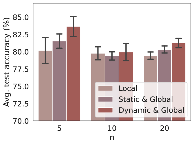
Figure 10. Effects of static and dynamic task feature extractor

We conducted a series of experiments in order to compare the effects of static and dynamic task feature extractors within our framework. These experiments were carried out on Cora dataset using non-overlapping settings. To accomplish this, we replaced our dynamic feature extractor, which distilled graphs based on the current model weights during each communication round, with a static extractor. This static extractor utilized a graph distillation method introduced in (Jin et al., 2022a) to ensure that the performance of the model training on the synthetic small graph closely approximated the ”final” performance achieved when training on the original, larger graph before the federated learning procedures. In this way, the static extractor offers static representations of tasks, which remain unchanged throughout the entire federated learning process. As shown in Figure 10, the dynamic task feature extractor is visually replaced by the static extractor for our experimental purposes. Notably, this replacement results in a 2.4% degradation in performance. The inferior performance of static task feature extractor comes from the unsatisfying local sample quality and quantity. Additionally, we compared the performance of the static extractor with a local training baseline and found that the static extractor still outperforms local learning.

Appendix D On the validity of $k$ in (11)

Below we state the result that $k$ in (11) is a valid kernel:

Proposition D.1.

The function $k$ is a valid kernel over the domain $[n]$.

Proof.

Let $\{\lambda_{1},\ldots,\lambda_{n}\}$ be the eigenvalues of $\mathbf{R}$. It then follows that the eigenvalues of $\mathbf{S}$ are $\{e^{t\lambda_{1}},\ldots,e^{t\lambda_{n}}\}$ which are non-negative, therefore $\mathbf{S}$ is positive semidefinite. The proposition follows by (Horn and Johnson, 2012, Theorem 7.5.9) ∎

References

- (1)
- Arivazhagan et al. (2019) Manoj Ghuhan Arivazhagan, Vinay Aggarwal, Aaditya Kumar Singh, and Sunav Choudhary. 2019. Federated learning with personalization layers. arXiv preprint arXiv:1912.00818 (2019).
- Baek et al. (2022) Jinheon Baek, Wonyong Jeong, Jiongdao Jin, Jaehong Yoon, and Sung Ju Hwang. 2022. Personalized Subgraph Federated Learning. In Proc. ICML.
- Bao et al. (2023) Wenxuan Bao, Haohan Wang, Jun Wu, and Jingrui He. 2023. Optimizing the Collaboration Structure in Cross-Silo Federated Learning. In Proc. ICML.
- Black et al. (2023) Mitchell Black, Zhengchao Wan, Amir Nayyeri, and Yusu Wang. 2023. Understanding oversquashing in gnns through the lens of effective resistance. In Proc. ICML. PMLR, 2528–2547.
- Chen et al. (2022b) Dexiong Chen, Leslie O’Bray, and Karsten Borgwardt. 2022b. Structure-aware transformer for graph representation learning. In International Conference on Machine Learning. PMLR, 3469–3489.
- Chen et al. (2022a) Fengwen Chen, Guodong Long, Zonghan Wu, Tianyi Zhou, and Jing Jiang. 2022a. Personalized federated learning with graph. In Proc. IJCAI.
- Chen et al. (2021) Shuxiao Chen, Qinqing Zheng, Qi Long, and Weijie J Su. 2021. A theorem of the alternative for personalized federated learning. arXiv preprint arXiv:2103.01901 (2021).
- Choromanski et al. (2020) Krzysztof Choromanski, Valerii Likhosherstov, David Dohan, Xingyou Song, Andreea Gane, Tamas Sarlos, Peter Hawkins, Jared Davis, Afroz Mohiuddin, Lukasz Kaiser, et al. 2020. Rethinking attention with performers. arXiv preprint arXiv:2009.14794 (2020).
- Dong et al. (2022) Tian Dong, Bo Zhao, and Lingjuan Lyu. 2022. Privacy for free: How does dataset condensation help privacy?. In International Conference on Machine Learning. PMLR, 5378–5396.
- Duan and Wang (2022) Yaqi Duan and Kaizheng Wang. 2022. Adaptive and robust multi-task learning. arXiv preprint arXiv:2202.05250 (2022).
- Fey and Lenssen (2019) Matthias Fey and Jan Eric Lenssen. 2019. Fast graph representation learning with PyTorch Geometric. arXiv preprint arXiv:1903.02428 (2019).
- Gilmer et al. (2017) Justin Gilmer, Samuel S. Schoenholz, Patrick F. Riley, Oriol Vinyals, and George E. Dahl. 2017. Neural Message Passing for Quantum Chemistry. In Proceedings of the 34th International Conference on Machine Learning (Proceedings of Machine Learning Research, Vol. 70), Doina Precup and Yee Whye Teh (Eds.). PMLR, International Convention Centre, Sydney, Australia, 1263–1272.
- Girvan and Newman (2002) Michelle Girvan and Mark EJ Newman. 2002. Community structure in social and biological networks. Proceedings of the national academy of sciences 99, 12 (2002), 7821–7826.
- Hanneke and Kpotufe (2022) Steve Hanneke and Samory Kpotufe. 2022. A no-free-lunch theorem for multitask learning. The Annals of Statistics 50, 6 (2022), 3119–3143.
- Hastie et al. (2009) Trevor Hastie, Robert Tibshirani, Jerome H Friedman, and Jerome H Friedman. 2009. The elements of statistical learning: data mining, inference, and prediction. Vol. 2. Springer.
- Horn and Johnson (2012) Roger A Horn and Charles R Johnson. 2012. Matrix analysis. Cambridge university press.
- Hu et al. (2020) Weihua Hu, Matthias Fey, Marinka Zitnik, Yuxiao Dong, Hongyu Ren, Bowen Liu, Michele Catasta, and Jure Leskovec. 2020. Open Graph Benchmark: Datasets for Machine Learning on Graphs. In Proc. NeurIPS. 22118–22133.
- Jang et al. (2016) Eric Jang, Shixiang Gu, and Ben Poole. 2016. Categorical reparameterization with gumbel-softmax. arXiv preprint arXiv:1611.01144 (2016).
- Jin et al. (2022a) Wei Jin, Xianfeng Tang, Haoming Jiang, Zheng Li, Danqing Zhang, Jiliang Tang, and Bing Yin. 2022a. Condensing graphs via one-step gradient matching. In Proc. ACM SIGKDD. 720–730.
- Jin et al. (2022b) Wei Jin, Lingxiao Zhao, Shichang Zhang, Yozen Liu, Jiliang Tang, and Neil Shah. 2022b. Graph Condensation for Graph Neural Networks. In Proc. ICLR.
- Kairouz et al. (2021) Peter Kairouz, H Brendan McMahan, Brendan Avent, Aurélien Bellet, Mehdi Bennis, Arjun Nitin Bhagoji, Kallista Bonawitz, Zachary Charles, Graham Cormode, Rachel Cummings, et al. 2021. Advances and open problems in federated learning. Foundations and Trends® in Machine Learning 14, 1–2 (2021), 1–210.
- Karimireddy et al. (2020) Sai Praneeth Karimireddy, Satyen Kale, Mehryar Mohri, Sashank Reddi, Sebastian Stich, and Ananda Theertha Suresh. 2020. Scaffold: Stochastic controlled averaging for federated learning. In International conference on machine learning. PMLR, 5132–5143.
- Kingma and Ba (2014) Diederik P Kingma and Jimmy Ba. 2014. Adam: A method for stochastic optimization. arXiv preprint arXiv:1412.6980 (2014).
- Kipf and Welling (2017) Thomas N Kipf and Max Welling. 2017. Semi-supervised classification with graph convolutional networks. In Proc. ICLR.
- Kondor and Lafferty (2002) Risi Imre Kondor and John Lafferty. 2002. Diffusion kernels on graphs and other discrete structures. In Proc. ICML, Vol. 2002. 315–322.
- Lehmann and Casella (2006) Erich L Lehmann and George Casella. 2006. Theory of point estimation. Springer Science & Business Media.
- Li et al. (2021) Tian Li, Shengyuan Hu, Ahmad Beirami, and Virginia Smith. 2021. Ditto: Fair and robust federated learning through personalization. In Proc. ICML. PMLR, 6357–6368.
- Li et al. (2020) Tian Li, Anit Kumar Sahu, Manzil Zaheer, Maziar Sanjabi, Ameet Talwalkar, and Virginia Smith. 2020. Federated optimization in heterogeneous networks. In Proc. MLSys, Vol. 2. 429–450.
- Long et al. (2023) Guodong Long, Ming Xie, Tao Shen, Tianyi Zhou, Xianzhi Wang, and Jing Jiang. 2023. Multi-center federated learning: clients clustering for better personalization. World Wide Web 26, 1 (2023), 481–500.
- Maddison et al. (2016) Chris J Maddison, Andriy Mnih, and Yee Whye Teh. 2016. The concrete distribution: A continuous relaxation of discrete random variables. arXiv preprint arXiv:1611.00712 (2016).
- McMahan et al. (2017) Brendan McMahan, Eider Moore, Daniel Ramage, Seth Hampson, and Blaise Aguera y Arcas. 2017. Communication-efficient learning of deep networks from decentralized data. In Proc. AISTATS. PMLR, 1273–1282.
- Pillutla et al. (2022) Krishna Pillutla, Kshitiz Malik, Abdel-Rahman Mohamed, Mike Rabbat, Maziar Sanjabi, and Lin Xiao. 2022. Federated learning with partial model personalization. In International Conference on Machine Learning. PMLR, 17716–17758.
- Ramezani et al. (2021) Morteza Ramezani, Weilin Cong, Mehrdad Mahdavi, Mahmut Kandemir, and Anand Sivasubramaniam. 2021. Learn Locally, Correct Globally: A Distributed Algorithm for Training Graph Neural Networks. In International Conference on Learning Representations.
- Sattler et al. (2020) Felix Sattler, Klaus-Robert Müller, and Wojciech Samek. 2020. Clustered federated learning: Model-agnostic distributed multitask optimization under privacy constraints. IEEE transactions on neural networks and learning systems 32, 8 (2020), 3710–3722.
- Shchur et al. (2018) Oleksandr Shchur, Maximilian Mumme, Aleksandar Bojchevski, and Stephan Günnemann. 2018. Pitfalls of graph neural network evaluation. arXiv preprint arXiv:1811.05868 (2018).
- Smith et al. (2017) Virginia Smith, Chao-Kai Chiang, Maziar Sanjabi, and Ameet S Talwalkar. 2017. Federated multi-task learning. Proc. NeurIPS 30 (2017).
- Tan et al. (2023) Yue Tan, Yixin Liu, Guodong Long, Jing Jiang, Qinghua Lu, and Chengqi Zhang. 2023. Federated learning on non-iid graphs via structural knowledge sharing. In Proc. AAAI, Vol. 37. 9953–9961.
- Tsai et al. (2019) Yao-Hung Hubert Tsai, Shaojie Bai, Makoto Yamada, Louis-Philippe Morency, and Ruslan Salakhutdinov. 2019. Transformer Dissection: An Unified Understanding for Transformer’s Attention via the Lens of Kernel. In Proc. EMNLP.
- Vaswani et al. (2017) Ashish Vaswani, Noam Shazeer, Niki Parmar, Jakob Uszkoreit, Llion Jones, Aidan N Gomez, Łukasz Kaiser, and Illia Polosukhin. 2017. Attention is all you need. Advances in neural information processing systems 30 (2017).
- Wang et al. (2018) Tongzhou Wang, Jun-Yan Zhu, Antonio Torralba, and Alexei A Efros. 2018. Dataset distillation. arXiv preprint arXiv:1811.10959 (2018).
- Woodworth et al. (2020) Blake Woodworth, Kumar Kshitij Patel, Sebastian Stich, Zhen Dai, Brian Bullins, Brendan Mcmahan, Ohad Shamir, and Nathan Srebro. 2020. Is local SGD better than minibatch SGD?. In International Conference on Machine Learning. PMLR, 10334–10343.
- Xie et al. (2021) Han Xie, Jing Ma, Li Xiong, and Carl Yang. 2021. Federated graph classification over non-iid graphs. In Proc. NeurIPS, Vol. 34. 18839–18852.
- Xu et al. (2023) Jian Xu, Xinyi Tong, and Shao-Lun Huang. 2023. Personalized Federated Learning with Feature Alignment and Classifier Collaboration. In Proc. ICLR.
- Xu et al. (2018) Keyulu Xu, Weihua Hu, Jure Leskovec, and Stefanie Jegelka. 2018. How powerful are graph neural networks? arXiv preprint arXiv:1810.00826 (2018).
- Yang et al. (2016) Zhilin Yang, William Cohen, and Ruslan Salakhudinov. 2016. Revisiting semi-supervised learning with graph embeddings. In Proc. ICML. PMLR, 40–48.
- Ye et al. (2023) Rui Ye, Zhenyang Ni, Fangzhao Wu, Siheng Chen, and Yanfeng Wang. 2023. Personalized Federated Learning with Inferred Collaboration Graphs. In Proc. ICML.
- Zhang et al. (2021) Ke Zhang, Carl Yang, Xiaoxiao Li, Lichao Sun, and Siu Ming Yiu. 2021. Subgraph federated learning with missing neighbor generation. In Proc. NeurIPS, Vol. 34. 6671–6682.
- Zhao et al. (2023) Xuyang Zhao, Huiyuan Wang, and Wei Lin. 2023. The Aggregation–Heterogeneity Trade-off in Federated Learning. In Proceedings of Thirty Sixth Conference on Learning Theory (Proceedings of Machine Learning Research, Vol. 195), Gergely Neu and Lorenzo Rosasco (Eds.). PMLR, 5478–5502. https://proceedings.mlr.press/v195/zhao23b.html
- Zhou et al. (2020) Yanlin Zhou, George Pu, Xiyao Ma, Xiaolin Li, and Dapeng Wu. 2020. Distilled one-shot federated learning. arXiv preprint arXiv:2009.07999 (2020).