Outlier-Insensitive Kalman Filtering:
Theory and Applications

Abstract

State estimation of dynamical systems from noisy observations is a fundamental task in many applications. It is commonly addressed using the linear kf (kf), whose performance can significantly degrade in the presence of outliers in the observations, due to the sensitivity of its convex quadratic objective function. To mitigate such behavior, outlier detection algorithms can be applied. In this work, we propose a parameter-free algorithm which mitigates the harmful effect of outliers while requiring only a short iterative process of the standard kf’s update step. To that end, we model each potential outlier as a normal process with unknown variance and apply online estimation through either expectation maximization or alternating maximization algorithms. Simulations and field experiment evaluations demonstrate our method’s competitive performance, showcasing its robustness to outliers in filtering scenarios compared to alternative algorithms.

I Introduction

State estimation from noisy observation is a core task in various signal processing applications [2], such as localization and tracking[3, 4, 5]. This task is commonly addressed by the celebrated kf [6], a recursive and efficient algorithm providing an optimal low-complexity solution under the Gaussian noise and linear dynamics assumptions. However, the kf’s performance degrades significantly when observations are impaired by outliers, due to its ls cost function [7, 8, 9]. In rw scenarios, measurements, especially from lower-quality sensors such as gnss (gnss) devices, often contain outliers [10, 11, 5]. This presents a significant challenge to the kf effectiveness. Therefore, an algorithm’s ability to remain insensitive to outliers plays a crucial role in state estimation missions. Various techniques were proposed in the literature to cope with outliers: basic techniques, such as those in [12, 13, 14], employ statistical tests like the ch2t to identify outliers based on prior information, and subsequently reject them. However, their robustness against outliers relies solely on the prediction step. The methods in [15, 16, 17] suggest reweighting the observation noise covariance at each update step, but they often require extensive hyper-parameter tuning. The approaches in [18, 19, 8, 20] strive to reduce the kf’s sensitivity to outliers by replacing its quadratic cost function. Specifically, the works [18, 19] propose a Huber-based kf by minimizing the combined $\mathcal{L}_{1}$ and $\mathcal{L}_{2}$ norms. The nominal noise is bounded using a Huber function, but the feature of heavy tails inherent in non-Gaussian noises could limit the estimation accuracy. The techniques in [8, 20] substitute the quadratic cost function with more suitable, often nonsmooth, convex functions, controlling outliers by promoting sparsity. However, these techniques involve smoothing algorithms rather than filtering and can be computationally complex. Methods such as [21] employ heavy-tailed distributions, like the sstd, to model the observation noise. However, in the absence of outliers, a significant degradation is expected due to the violated Gaussian assumption. The authors of [22] address this problem by using a hierarchical distribution, specifically adopting a more robust distribution when the noise is skewed. With recent advancements in nn, methods such as [14, 23] suggest detecting and correcting outlier observations using nn before they enter into the kf stage. Nonetheless, these methods often require access to large amounts of data and pre-training. In [24], the use of nuv (nuv) prior is introduced to devising an outlier insensitive ks (ks). Inspired by sparse Bayesian learning [25, 26], the authors propose to model each potential outlier as nuv [27, 28, 29], and estimate the unknown variance using em (em) algorithm [30, 31], resulting in sparse outlier detection. The main advantages of this approach are that it $(i)$ is parameter-free; $(ii)$ amounts to a short iterative process within the ks’s update step; and $(iii)$ effectively leverages all observation samples during the state estimation process of the ks. In [24] focuses on the offline smoothing task and proposes only the derivation of the em to estimate the unknown variance, which requires the computation of second-order moments.

In this work, we introduce oikf (oikf), which is designed for the more commonly encountered task of online real-time filtering. In addition to presenting the em algorithm, we also provide the am (am) algorithm [32] for estimating the unknown variance, which eliminates the need for computing the second-order moment of the state vector, making its implementation simpler. Specifically, the contributions of this paper are:

1. Motivation: A comprehensive motivation for the utilization of nuv in outlier detection within the kf framework, highlighting its benefits.

2. Theory: A comprehensive elucidation of the motivation behind the nuv prior representation to model outlier and tackle the problem of state estimation in the presence of outliers. To that end, we provide a complete mathematical derivation providing in-depth insights into the theoretical aspects of our oikf with its two implementations oikf-em and oikf-am.

3. Extensive Simulation Analysis: a comparison for scenarios with low outlier intensity, suitable for any sensor updating the kf, which are inherently more challenging to detect and compensate for.

4. gnss Outlier Detection: A real-world analysis focused on gnss outlier detection using two datasets with three different platforms to highlight our approach robustness. One dataset comprises of Segway recordings [33], while the other comprises data from a quadrotor and a marine vessel [34].

5. Open Source: The source code and additional information on our empirical study can be found at https://github.com/KalmanNet/OIKF-NUV.git.

The rest of this paper is organized as follows: Section II reviews the preliminaries for the or state estimation task. Section III provides detailed explanations of nuv modeling and its utilization in the oikf. Section IV presents the results of the empirical study, while Section V concludes the paper with final remarks.

II Problem Formulation and Preliminaries

In this section, we introduce the preliminaries for the task of or online state estimation, namely, the ss (ss) model with outliers, and recapitulate the kf algorithm.

II-A State Space Model with Outliers

We consider a scenario where noisy time-series observations, denoted as $\{\mathbf{y}_{\tau}\}_{\tau=1}^{t}$, are sequentially presented to a filter. The objective is to provide a sequence of estimates, $\{\hat{\mathbf{x}}_{\tau}\}_{\tau=1}^{t}$, corresponding to a sequence of hidden (latent) values or ’states’, $\{\mathbf{x}_{\tau}\}_{\tau=1}^{t}$ [35]. This scenario introduces an additional challenge: a subset of the observations may be impaired by outliers from an unknown distribution. We operate under the assumption that an anomalous observation should be considered a rare event to qualify as an outlier.

Unlike the offline state estimation task, aka as smoothing, which is considered in [36], where all observations are provided as a batch, we focus on rt filtering here. In this approach, the estimate of $\mathbf{x}_{t}$ relies solely on current and past observations. This stands in contrast to the methodology in [24], where iterating on the entire batch of observations is used to enhance robustness to outliers and consequently improve state estimation performance.

In this work, we assume that the underlying relationship between the observed values and the hidden values is represented by a ss model [2]. We focus on a lg ss model in dt, $t\in\mathbb{Z}$, represented as follows:

$$\mathbf{x}_{t} =\mathbf{F}\cdot{\mathbf{x}_{t-1}}+\mathbf{e}_{t},\quad\,\,\,\,\,\,\mathbf{e}_{t}\sim\mathcal{N}\left(\mathbf{0},\mathbf{Q}\right),\quad\mathbf{x}_{t}\in\mathbb{R}^{m}$$ (1a)

$$\mathbf{y}_{t} =\mathbf{H}\cdot\mathbf{x}_{t}+\mathbf{z}_{t}+\mathbf{u}_{t},\,\,\,\,\mathbf{z}_{t}\sim\mathcal{N}\left(\mathbf{0},\mathbf{R}\right),\quad\mathbf{y}_{t}\in\mathbb{R}^{n}.$$ (1b)

Equation (1a) describes the time evolution of the state $\mathbf{x}_{t}$ from the previous state $\mathbf{x}_{t-1}$, governed by an system (evolution) matrix $\mathbf{F}$ and agn $\mathbf{e}_{t}$. This noise, with a process covariance matrix $\mathbf{Q}$, represents potential modeling uncertainties. Equation (1b) portrays how observations $\mathbf{y}_{t}$ are generated from $\mathbf{x}_{t}$, the current state at time step $t$. This process involves a measurement (observation) matrix $\mathbf{H}$, agn $\mathbf{z}_{t}$, with a measurement covariance matrix $\mathbf{R}$ accounting for uncertainties in the measurements, and potential outliers $\mathbf{u}_{t}$, which follows an unspecified distribution.

II-B Linear Kalman Filtering

The celebrated kf [6] is particularly noteworthy for its recursive and efficient algorithm, providing an optimal solution under Gaussian noise and linear dynamics [37, 2]. In its most general form, the kf aims to estimate the current state based on a noisy observation signal. However, the kf’s performance can degrade in the presence of outliers [8, 9, 20]. This sensitivity stems from the filter’s objective to minimize a quadratic cost function, a structure that inherently is not able to follow fast jumps in the state dynamics[38]. For full details on how the map (map) formulation boils down to ls minimization, see[39, 40].

The kf estimates the state $\mathbf{x}_{t}$ from the observations $\left\{\mathbf{y}_{\tau}\right\}_{{\tau\leq t}}$ and can be thought of as a two-step process at each time step: predict and update. In the predict step, the joint probability distribution is computed using the first and second-order moments of the Gaussian distribution, resulting in the prior distribution. The predict of the $1^{\textrm{st}}$ and $2^{\textrm{nd}}$ order moments:

$$\hat{\mathbf{x}}_{t\left|t-1\right.} =\mathbf{F}\cdot{\hat{\mathbf{x}}_{t-1}},\hskip 12.80365pt\bm{\Sigma}_{t\left|t-1\right.}\!=\!\mathbf{F}\cdot\bm{\Sigma}_{t-1}\cdot\mathbf{F}^{\top}\!+\!\mathbf{Q},$$ (2a)

$$\hat{\mathbf{y}}_{t\left|t-1\right.} =\mathbf{H}\cdot{\hat{\mathbf{x}}_{t\left|t-1\right.}},\hskip 5.69046pt\mathbf{S}_{t\left|t-1\right.}\!=\!\mathbf{H}\cdot\bm{\Sigma}_{t\left|t-1\right.}\cdot\mathbf{H}^{\top}\!+\!\mathbf{R}.$$ (2b)

where $\bm{\Sigma}$ represents the covariance of the state, $\mathbf{F}$ is the state-transition model, and $\mathbf{H}$ is the observation and model. The matrices $\mathbf{Q}$ and $\mathbf{R}$ are the covariance matrices of the process noise and observation noise, respectively. The kf uses this prior distribution in the update step in the posterior distribution calculation by computing the new observation $\mathbf{y}_{t}$ with the previously predicted prior $\hat{\mathbf{x}}_{t\left|t-1\right.}$. And the update of the $1^{\textrm{st}}$ and $2^{\textrm{st}}$ order statistical moment

$$\hat{\mathbf{x}}_{t}=\hat{\mathbf{x}}_{t\left|t-1\right.}+\mathbfcal{K}_{t}\cdot\Delta\mathbf{y}_{t},\quad{\bm{\Sigma}}_{t}\!=\!{\bm{\Sigma}}_{t\left|t-1\right.}\!-\!\mathbfcal{K}_{t}\cdot{\mathbf{S}}_{t\left|t-1\right.}\cdot\mathbfcal{K}^{\top}_{t},$$ (3)

$$\mathbfcal{K}_{t}={\bm{\Sigma}}_{t\left|t-1\right.}\cdot{\mathbf{H}^{\top}}\cdot{\mathbf{S}}^{-1}_{t\left|t-1\right.},\quad\Delta\mathbf{y}_{t}=\mathbf{y}_{t}-\hat{\mathbf{y}}_{t\left|t-1\right.}.$$ (4)

where $\mathbfcal{K}_{t}$ is the Kalman gain matrix used to balance the contributions of both parts and produce the final posterior distribution.

III Outlier-Insensitive Kalman Filtering Using NUV Prior

This section introduces our oikf algorithm. First, we present the motivation behind using nuv prior representation for outlier detection in kf. Then, we elaborate on our innovative approach of integrating the nuv prior into the kf algorithm for outlier detection, denoted as oikf. Finally, we provide a comprehensive derivation of our two proposed algorithms to estimate the unknown variance of the nuv, namely nuv-based em and nuv-based am.

III-A Motivation For NUV Prior Representation

The nuv formulation models a variable of interest as a normal distribution with unknown variance, given that the unknown variance has a prior distribution [27, 29]. The nuv representation method proves to be a robust approach with various applications, each encountering different problems, and the choice of a specific prior depends on its circumstances. For example, [41] proposes different priors for computer imaging problems. In our specific problem, outlier-insensitive kf, we opt for a uniform prior. This choice is motivated by computational convenience and the objective of resulting in sparse outlier detection, as explained in Subsection III-C and in Subsection III-E. Once the prior is set, our approach is in-fact a parameter free approach.

One well-known property of the nuv is its tendency to yield a non-convex penalty [28], suitable for addressing sparse least-squares problems with outliers. This non-convex penalty is motivated by the influence function [42] in residuals. This function assesses the effect of a residual’s size on the loss by evaluating its derivative [20]. As the size of the residuals increases, the influence function gradually approaches zero, leading to a sparse solution.

To motivate, we employ a simple example, based on the observation model (1b), which illustrates the fundamental property of nuv priors. Consider a single observation of the form

$$\mathrm{y}=\mathrm{v}+\mathrm{u},\quad\mathrm{y}\in\mathbb{R}$$ (5)

Here, $\mathrm{v}$ is an awgn (awgn) with variance $\mathrm{r}^{2}$. The variable of interest $\mathrm{u}$ is modeled as a zero-mean real scalar Gaussian random variable with an unknown variance $\gamma^{2}$ (nuv). The mle (mle) of $\gamma^{2}$ from a single sample $\mathrm{y}\in\mathbb{R}$ can be computed as follows:

$$\hat{\gamma}^{2}=\operatorname*{arg\,max}_{\gamma^{2}\geq 0}\mathcal{P}\left(\mathrm{y}\left|\gamma^{2}\right.\right)\mathcal{P}\left(\gamma^{2}\right)$$ (6)

when we assume a constant prior $\mathcal{P}\left(\gamma^{2}\right)=\sqrt{2\pi}$ for computation convenience and $\mathcal{P}\left(\mathrm{y}\left|\gamma^{2}\right.\right)$ is normally distributed, that is $\mathcal{P}\left(\mathrm{y}\left|\gamma^{2}\right.\right)\sim\mathcal{N}\left(0,\mathrm{r^{2}+\gamma^{2}}\right)$, then (6) can be rewritten as:

$$\hat{\gamma}^{2}=\operatorname*{arg\,max}_{\gamma^{2}\geq 0}\left\{\frac{1}{\sqrt{2\pi\left(\mathrm{r}^{2}+\gamma^{2}\right)}}\exp\left(\frac{-\mathrm{y}^{2}}{2(\mathrm{r}^{2}+\gamma^{2})}\right)\right\}$$ (7)

To simplify the computation of (7) is written in terms of a logarithmic function:

$$\hat{\gamma}^{2}=\operatorname*{arg\,min}_{{\gamma^{2}}\geq 0}\left\{\ln\left(\mathrm{r}^{2}+\gamma^{2}\right)+\frac{{\mathrm{y}^{2}}}{\left(\mathrm{r}^{2}+\gamma^{2}\right)}\right\}.$$ (8)

In order to derive (8), we equate its derivative with regard to ${\gamma^{2}}$ to zero and we get the closed form of unknown variance $\gamma^{2}$ of Gaussian $\mathrm{u}$:

$$\hat{\gamma}^{2}=\max\left\{\mathrm{y}^{2}-\mathrm{r}^{2},0\right\}.$$ (9)

In a subsequent step, assuming $\gamma^{2}$ is estimated as $\hat{\gamma}^{2}$ as in (9), the map estimate of $\mathrm{u}$, denoted as $\hat{\mathrm{u}}$, is given by:

$$\hat{\mathrm{u}}=\operatorname*{arg\,max}_{\mathrm{u}}\mathcal{P}\left(\mathrm{y}\left|\mathrm{u}\right.\right)\cdot\mathcal{P}\left(\mathrm{u}\right)$$ (10)

when $\mathcal{P}\left(\mathrm{y}\left|\mathrm{u}\right.\right)\sim\mathcal{N}\left(\mathrm{u},\mathrm{r}^{2}\right)$ and $\mathcal{P}\left(\mathrm{u}\sim\mathcal{N}\left(0,\gamma^{2}\right)\right)$, the derivation of $\hat{\mathrm{u}}$ can be accomplished simper to $\gamma^{2}$ in (9), thus,

$$\hat{\mathrm{u}}= \operatorname*{arg\,max}_{\mathrm{u}}\left\{\frac{1}{\sqrt{2\pi\mathrm{r}^{2}}}e^{\frac{-\left(\mathrm{y}-\mathrm{u}\right)^{2}}{2\mathrm{r}^{2}}}+\frac{1}{\sqrt{2\pi\gamma^{2}}}e^{\frac{-\mathrm{u}^{2}}{2\gamma^{2}}}\right\}$$ (11)

$$= \underset{\mathrm{u}}{\arg\min}\,\left\{\frac{\left(\mathrm{y}-\mathrm{u}\right)^{2}}{2\mathrm{r}^{2}}+\frac{{\mathrm{u}}^{2}}{2\gamma^{2}}\right\}.$$

Maximizing the expression in (11) results in

$$\mathrm{\hat{u}}= \mathrm{y}\cdot\frac{\hat{\gamma}^{2}}{\hat{\gamma}^{2}+\mathrm{r}^{2}}=\max\left\{\frac{\mathrm{y}^{2}-\mathrm{r}^{2}}{\mathrm{y}},0\right\}.$$ (12)

Plugging the obtained result (9) into $\mathcal{P}\left(\mathrm{y}\right)$:

$$\mathcal{P}\left(\mathrm{y}\right)=\max_{\gamma^{2}\geq 0}\mathcal{P}\left(\mathrm{y}\left|\gamma\right.^{2}\right)\cdot\mathcal{P}\left(\gamma^{2}\right)$$ (13)

yields the equivalent cost function $\mathcal{L}\left(\mathrm{y}\right)=-\log\,\mathcal{P}\left(\mathrm{y}\right)$, when $\mathcal{P}\left(\mathrm{y}\right)$ can be derived from (8) when we also assume a constant prior for $\mathcal{P}\left(\gamma^{2}\right)$, and we obtain:

$$\mathcal{L}\left(\mathrm{y}\right)= -\log\left[\frac{1}{\sqrt{\mathrm{r}^{2}+\gamma^{2}}}\exp\left(\frac{-y^{2}}{\mathrm{r^{2}}+\gamma^{2}}\right)\right]$$ (14)

$$= \frac{1}{2}\log\left(\mathrm{r^{2}}+\gamma^{2}\right)+\frac{\mathrm{y^{2}}}{\mathrm{r^{2}+\gamma^{2}}}$$

Using the obtained expression for $\hat{\gamma}^{2}$ from (9), we obtain:

$$\mathcal{L}\left(\mathrm{y}\right)=\begin{cases}\mathrm{y}^{2}/\left(2\mathrm{r}^{2}\right)+\log\,\mathrm{r},&{\mathrm{y}^{2}}<\mathrm{r}^{2}\\ \log\left\lvert\mathrm{y}\right\rvert+0.5,&{\mathrm{y}^{2}}\geq\mathrm{r}^{2}\end{cases}$$ (15)

If $\mathrm{r}>0$, (15) results in a nonconvex function, which proves valuable for handling sparse ls models, such as kf, in the presence of outliers[28].
Through this example, we establish that $\gamma^{2}=0$ leads to $\mathrm{u}=0$, indicating that no outlier is identified and the obtained $\gamma^{2}$ leads to a nonconvex cost function.

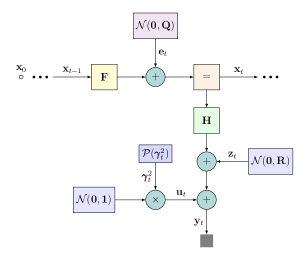
Figure 1: Factor graph of the system model at time step $t$

III-B Kalman Filtering with NUV Prior

The proposed oikf introduces a new form of the ss model (1) by incorporating an additional variable into the observation signal, denoted as $\mathbf{u}_{t}$. This variable $\mathbf{u}_{t}$ represents the impulsive noise responsible for causing outliers. To improve the model’s capability to handle heavy-tailed distributions in observations, we model this outlier $\mathbf{u}_{t}$ as nuv ${\boldsymbol{\gamma}}^{2}_{t}$, namely:

$$\mathbf{u}_{t}\sim\mathcal{N}(0,{\boldsymbol{\gamma}}^{2}_{t}),\quad{\boldsymbol{\gamma}}^{2}_{t}\sim\mathcal{P}\left({\boldsymbol{\gamma}}^{2}_{t}\right)$$ (16)

where $p({\boldsymbol{\gamma}}^{2}_{t})$ is the prior distribution of ${\boldsymbol{\gamma}}^{2}_{t}$. Figure 1 demonstrates visually the integration of the nuv representation into the overall model through a factor graph. The nuv representation approach results in a sparse outlier detection solution [27, 29], indicating that most values of $\boldsymbol{\gamma}^{2}_{t}$ will be zero. Consequently, as can be seen in (12) this leads to $\mathbf{u}_{t}=0$, suggesting the absence of outliers, as expected.
For any given observation sample $\mathbf{y}_{t}$ (1b), we define $\mathbf{v}_{t}$ to be the error vector as the sum of two independent sources: the observation noise $\mathbf{z}_{t}$ and the outlier noise $\mathbf{u}_{t}$. Thus, the covariance matrix of $\mathbf{v}_{t}$ is equal by definition:

$$\mathbf{v}_{t}\triangleq\mathbf{y}_{t}-\mathbf{H}\cdot\mathbf{x}_{t}=\mathbf{z}_{t}+\mathbf{u}_{t},\quad\mathbf{v}_{t}\sim\mathcal{N}\left(\mathbf{0},\mathbf{\Gamma}_{t}\right)$$ (17)

$\mathbf{\Gamma}_{t}$ is diagonal and comprises the sum of variances of the two noise sources, namely

$$\mathbf{\Gamma}_{t}=\textrm{diag}\left({\bm{\nu}}^{2}_{t}\right),\quad{\bm{\nu}}^{2}_{t}\triangleq\mathbf{r}^{2}+{\boldsymbol{\gamma}}^{2}_{t}.$$ (18)

In each kf iteration, the temporary estimate of $\boldsymbol{\gamma}^{2}_{t}$ is incorporated into the overall covariance $\mathbf{\Gamma}_{t}$, effectively reweighting the covariance noise of the observations. Consequently, this affects the Kalman gain $\mathbfcal{K}_{t}$ in the update equations, allowing to extract the information from all the noisy observations and leverage their information effectively.

For the process of map estimation of the unknown variance, ${\boldsymbol{\gamma}}^{2}_{t}$, we can apply either em (Subsection III-C) or am (Subsection III-D) algorithms. While in the em approach, the second-order moment $\bm{\nu}_{t}$ (18) is directly estimated, in the am approach, it is obtained from estimating the first-order moment $\mathbf{v}_{t}$ (17) only, as summarized below:

$${\hat{\boldsymbol{\gamma}}}^{2}_{t}=\max\left\{\bm{\nu}_{t}^{2}-\mathbf{r}^{2},0\right\},\hskip 4.97931pt\bm{\nu}_{t}^{2}=\left\{\textrm{EM}:\hat{\bm{\nu}}_{t}^{2},\textrm{AM}:\mathbf{\hat{v}}^{2}_{t}\right\}.$$ (19)

For both approaches, an outlier is detected when $\hat{\boldsymbol{\gamma}}^{2}_{t}\neq 0$, otherwise, when $\hat{\boldsymbol{\gamma}}^{2}_{t}=0$, it implies no outlier is present and we revert to the standard kf, preserving its optimally for data without outliers.

III-C Expectation Maximization

For an observation $\mathbf{y}_{t}$, and the state vector $\mathbf{x}_{t}$ as defined in (1), the map estimation for the unknown variance $\hat{\boldsymbol{\gamma}}^{2}_{t}$ is

$$\hat{\boldsymbol{\gamma}}^{2}_{t}\left(\mathbf{y}_{t}\right) =\underset{\boldsymbol{\gamma}^{2}_{t}\geq 0}{\arg\max}\,\mathcal{P}\left(\boldsymbol{\gamma}^{2}_{t}\left|\mathbf{y_{t}}\right.\right)=\underset{\boldsymbol{\gamma}^{2}_{t}\geq 0}{\arg\max}\,\mathcal{P}\left(\mathbf{y}_{t}\left|{\boldsymbol{\gamma}^{2}_{t}}\right.\right)\cdot\mathcal{P}\left({\boldsymbol{\gamma}^{2}_{t}}\right)$$

$$=\underset{\boldsymbol{\gamma}^{2}_{t}\geq 0}{\arg\max}\,\int\mathcal{P}\left(\mathbf{y}_{t},\mathbf{x}_{t}\left|{\boldsymbol{\gamma}^{2}_{t}}\right.\right)dx\cdot\mathcal{P}\left({\boldsymbol{\gamma}^{2}_{t}}\right)$$ (20)

To solve the optimization problem in (20), we devise the iterative em algorithm, which consists of two iterating steps, namely, E-step and M-step.
The E-step determines the conditional expectation:

$$\mathds{E}_{\mathbf{x}_{t}\left|\left({\boldsymbol{\gamma}^{i-1}_{t}}\right)^{2},\mathbf{y}_{t}\right.}\left[\log\left(\mathcal{P}\left({\mathbf{y}_{t},\mathbf{x}_{t}}\left|\boldsymbol{\gamma}\right._{t}^{2}\right)\cdot\mathcal{P}\left(\boldsymbol{\gamma}^{2}_{t}\right)\right)\right]=$$ (21)

$$\mathds{E}_{\mathbf{x}_{t}\left|\left({\boldsymbol{\gamma}^{i-1}_{t}}\right)^{2},\mathbf{y}_{t}\right.}\left[\log{\mathcal{P}\left(\mathrm{y}_{t}\left|\mathbf{x}_{t},\boldsymbol{\gamma}^{2}_{t}\right.\right)}+\mathcal{P}\left(\mathbf{x}_{t}\left|\boldsymbol{\gamma}^{2}_{t}\right.\right)+\log{\mathcal{P}\left(\boldsymbol{\gamma}^{2}_{t}\right)}\right]$$

Using the Markov property and the structure of the ss model, the term $\mathcal{P}\left(\mathbf{x}_{t}\left|\boldsymbol{\gamma}^{2}_{t}\right.\right)$ is can be rewritten as $\mathcal{P}\left(\mathbf{x}_{t}\left|\mathbf{x}_{t-1}\right.\right)$.

The M-step goal is to maximize (21) with respect to ${\boldsymbol{\gamma}^{2}_{t}}$. In this problem, we assume a uniform prior on the unknown variance [27]:

$$\mathcal{P}\left({\boldsymbol{\gamma}^{2}_{t}}\right)\propto 1$$ (22)

The choice of $\mathcal{P}\left({\boldsymbol{\gamma}^{2}_{t}}\right)$ to be uniform is one of many options. As stated in [28], a uniform prior on $\mathcal{P}\left({\boldsymbol{\gamma}^{2}_{t}}\right)$, also known as plain nuv, eventually leads to a non-convex cost function which results in the sparse effect of the unknown variance, with most of them being zeros, as expected.

Since $\mathcal{P}\left({\boldsymbol{\gamma}^{2}_{t}}\right)$ and the evolution $\mathcal{P}\left(\mathbf{x}_{t}\left|\mathbf{x}_{t-1}\right.\right)$ do not depend on ${\boldsymbol{\gamma}^{2}_{t}}$, they can thus be omitted from the optimization process (21) and we can evaluate the standard em and compute the conditional distribution in (21). Thus, the $i$th iteration step is derived by:

$$Q\left[\left(\boldsymbol{\gamma}^{i}_{t}\right)^{2}\right]=\mathds{E}_{\mathbf{x}_{t}\left|\left(\boldsymbol{\gamma}^{i-1}_{t}\right)^{2},\mathbf{y}_{t}\right.}\left[\log{\mathcal{P}\left(\mathbf{y}_{t}\left|\mathbf{x}_{t},\boldsymbol{\gamma}^{2}_{t}\right.\right)}\right]$$

$$= \mathds{E}_{\mathbf{x}_{t}\left|\left(\boldsymbol{\gamma}^{i-1}_{t}\right)^{2},\mathbf{y}_{t}\right.}\left[\log\left(\frac{1}{\sqrt{\mathbf{\Gamma}_{t}}}\cdot\mathrm{exp}\left(\frac{-\left(\mathbf{y}_{t}-\mathbf{H}\cdot\mathbf{x}_{t}\right)^{2}}{2\cdot\mathbf{\Gamma}_{t}}\right)\right)\right]$$

$$\propto \log{\mathbf{\Gamma}_{t}}+\frac{1}{{\mathbf{\Gamma}_{t}}}\cdot\mathds{E}_{\mathbf{x}_{t}\left|\left(\boldsymbol{\gamma}^{i-1}_{t}\right)^{2}\right.,\mathbf{y}_{t}}\left[\left(\mathbf{y}_{t}-\mathbf{H}\cdot\mathbf{x}_{t}\right)^{2}\right].$$ (23)

To expand the term $\mathds{E}_{\mathbf{x}_{t}\left|\left(\boldsymbol{\gamma}^{i-1}_{t}\right)^{2}\right.,\mathbf{y}_{t}}\left[\left(\mathbf{y}_{t}-\mathbf{H}\cdot\mathbf{x}_{t}\right)^{2}\right]$,we utilize the kf, allowing to obtain the first- and second-order posterior moments of $\mathbf{x}_{t}$, which equal by definition:

$$\mathds{E}_{\mathbf{x}_{t}\left|\left(\boldsymbol{\gamma}^{i-1}_{t}\right)^{2},\mathbf{y}_{t}\right.}\left(\mathbf{x}_{t}\right)\triangleq\hat{\mathbf{x}}_{t}^{i},$$ (24)

$$\mathds{E}_{\mathbf{x}_{t}\left|\left(\boldsymbol{\gamma}^{i-1}_{t}\right)^{2},\mathbf{y}_{t}\right.}\left(\mathbf{x}_{t}\cdot\mathbf{x}_{t}^{\top}\right)=\bm{\Sigma}^{i}_{t}+\mathbf{X}_{t}^{\text{II}}\triangleq{\hat{\mathbf{X}}_{t}^{i}}.$$

To simplify computations, the following expressions are equal by definition:

$$\mathbf{X}_{t}^{\text{II}}\triangleq\mathbf{\hat{x}}^{i}_{t}\cdot{\mathbf{\hat{x}}^{i}_{t}}^{\top},\quad\mathbf{Y}_{t}^{\text{II}}\triangleq\mathbf{y}_{t}\cdot\mathbf{y}_{t}^{\top},$$ (25)

$$\mathbf{XY}_{t}\triangleq\mathbf{\hat{x}}^{i}_{t}\cdot\mathbf{y}_{t}^{\top},\quad\mathbf{YX}_{t}\triangleq\mathbf{y}_{t}\cdot{\mathbf{\hat{x}}^{i}_{t}}^{\top},$$

Finally, the expectation step (23) is reduced to the following expression:

$$Q\left[\left(\boldsymbol{\gamma}^{i}_{t}\right)^{2}\right]=\log{\mathbf{\Gamma}_{t}}+\frac{1}{{\mathbf{\Gamma}_{t}}}\cdot\mathbf{V}_{t}$$ (26)

where $\mathbf{V}_{t}$ is equal by definition:

$$\mathbf{V}_{t}\triangleq\left\{\mathbf{Y}_{t}^{\text{II}}-\mathbf{H}\cdot\mathbf{XY}_{t}-\mathbf{YX}_{t}\cdot\mathbf{H}^{\top}-\mathbf{H}\cdot{\hat{\mathbf{X}}_{t}^{i}}\cdot\mathbf{H}^{\top}\right\}$$ (27)

In M-Step, we maximize (26) w.r.t. to $\mathbf{\Gamma}_{t}$, thus for the $i$-th iteration:

$${\hat{\mathbf{\Gamma}}^{i}_{t}}=\operatorname*{arg\,max}_{\mathbf{\Gamma}^{2}_{t}\geq 0}\biggl{\{}\ln{\mathbf{\Gamma}_{t}}+\frac{1}{\mathbf{\Gamma}_{t}}\cdot\mathbf{V}_{t}\biggl{\}}=\mathbf{V}_{t}$$ (28)

We further exploit the fact that $\mathbf{{\Gamma}}_{t}$ in (18) is diagonal, to expand $\mathbf{{\Gamma}}_{t}$ to its components and estimate the variance $\left(\mathrm{\hat{\nu}}^{i}_{t,k}\right)^{2}$ for each dimension $k\in\{1,\dots,n\}$ in a scalar manner using (27)

$$\left(\hat{\nu}^{i}_{t,k}\right)^{2}=\mathbf{y}_{t,k}^{2}-2\cdot{\mathbf{y}_{t,k}}\cdot\mathbf{H}\cdot\hat{\mathbf{x}}_{t,k}^{i}+\mathbf{H}\cdot\left(\hat{\mathbf{x}}_{t,k}^{i}\right)^{\textrm{II}}\cdot\mathbf{H}^{\top}$$ (29)

when $\hat{\mathrm{x}}_{t}$ is the posteriori state estimate. From (18), (29) and the fact that variance must be positive, we can calculate ${\gamma}_{t,k}^{2}$ in the $i$th iteration:

$$\left({\hat{\gamma}}^{i}_{t,k}\right)^{2}=\max\left\{\left({\hat{\nu}}^{i}_{t,k}\right)^{2}-\mathrm{r}_{k}^{2},0\right\}.$$ (30)

Thus, when an outlier is detected at a time step $t$, $\gamma^{2}_{t,k}>0$ otherwise its $0$, which may lead to a sparse solution. As a consequence, the outlier will be estimated as $\mathrm{\hat{u}}_{t,k}=0$.

The above procedure is repeated iteratively for a fixed $\operatorname*{\textit{K}}$ iterations, or until convergence is achieved. Algorithm 1 provides the suggested pseudo-code for the oikf based nuv-em.

Algorithm 1 oikf based nuv-em for time instance $t$

1:Number of iterations $\operatorname*{\textit{K}}$

2:Predict: Estimate a priori for $\mathbf{\hat{x}}_{t\left|t-1\right.}^{i=0},\mathbf{\bm{\Sigma}}_{t\left|t-1\right.}^{i=0}$ via (2a)

3:for $i=0,...,\operatorname*{\textit{K}}-1$ do

4:    EM: Estimate $\left(\hat{\boldsymbol{\gamma}}^{i}_{t}\right)^{2}$ via (30) with the $2$nd-order

5:              moment ${\hat{\mathbf{X}}_{t}^{i}}$ as in (24)

6:    Compute $\mathbf{\Gamma}_{t}^{i}=\textnormal{diag}\left(\mathbf{r}^{2}+\left(\hat{\boldsymbol{\gamma}}^{i}_{t}\right)^{2}\right)$

7:    Compute $\mathbf{\hat{y}}_{t\left|t-1\right.}^{i},\mathbf{S}_{t\left|t-1\right.}^{i}$ via  (2b) with $\mathbf{R}=\mathbf{\Gamma}_{t}^{i}$.

8:    Update: Estimate a posteriori for $\mathbf{\hat{x}}_{t}^{i},\bm{\Sigma}_{t}^{i}$ via (3)

9:end for

III-D Alternating Maximization

As in the EM approach, our goal is to estimate $\boldsymbol{\gamma}^{2}_{t}$ but here using am instead. To that end, we employ the iterative am algorithm based on the plain smoothed nuv [28] to compute the joint map estimate for $\boldsymbol{\gamma}^{2}_{t}$, when the variable of interest is $\mathbf{v}_{t}$. Consider the use of a nuv prior on variable $\mathbf{v}_{t}$ in a ss model with observation $\mathbf{y}_{t}$, we aim to determine their joint MAP estimate:

$$[\hat{\mathbf{v}}_{t},\hat{{\boldsymbol{\gamma}}}^{2}_{t}](\mathbf{y}_{t}) =\operatorname*{arg\,max}_{\mathbf{v}_{t},\boldsymbol{\gamma}^{2}_{t}\geq 0}\mathcal{P}\left(\mathbf{y}_{t},\mathbf{v}_{t},\boldsymbol{\gamma}^{2}_{t}\right)$$

$$\!=\!\underset{{\mathbf{v}_{t},\boldsymbol{\gamma}^{2}_{t}\geq 0}}{\arg\max}\,\mathcal{P}\left({\mathbf{y}_{t}\left|\mathbf{v}_{t}\right.}\right)\cdot\mathcal{P}\left(\mathbf{v}_{t}\big{|}{\boldsymbol{\gamma}^{2}_{t}}\right)\cdot\mathcal{P}\left(\boldsymbol{\gamma}^{2}_{t}\right).$$ (31)

The latter is valid because as for certain continuous random variables, the joint probability density function is defined as the derivative of the joint cumulative distribution function.

To compute (31), we derive the am algorithm, which iterates between a maximization step over the error state ${\mathbf{v}}_{t}$ with a fixed variance ${\boldsymbol{\gamma}^{2}_{t}}$:

$$\hat{\mathbf{v}}_{t}\!=\!\underset{{\mathbf{v}_{t}}}{\arg\max}\,\mathcal{P}\left({\mathbf{y}_{t}\left|\mathbf{v}_{t}\right.}\right)\cdot\mathcal{P}\left(\mathbf{v}_{t}\left|\boldsymbol{\gamma}\right.^{2}_{t}\right)$$ (32)

In particular, we replace $\mathbf{v}_{t}$ in (31) with its instantaneous estimate $\mathbf{\hat{v}}_{t}^{i}=\mathbf{y}_{t}-\mathbf{H}\cdot\mathbf{\hat{x}}_{t}^{i}$, which can be extracted from the kf. The next step in the am is maximization (31) over the unknown variance ${\boldsymbol{\gamma}^{2}_{t}}$ based on $\mathbf{v}_{t}$, resulting in

$$\hat{\boldsymbol{\gamma}}^{2}_{t}=\underset{{\boldsymbol{\gamma}^{2}_{t}}\geq 0}{\arg\max}\,\mathcal{P}\left(\mathbf{v}_{t}\left|\boldsymbol{\gamma}\right.^{2}_{t}\right)\cdot\mathcal{P}\left(\boldsymbol{\gamma}^{2}\right).$$ (33)

Note that since $\mathcal{P}\left({\mathbf{y}_{t}\left|\mathbf{v}_{t}\right.}\right)$ doesn’t depend on ${\boldsymbol{\gamma}}^{2}_{t}$, and as we assume a uniform prior for $\mathcal{P}\left(\boldsymbol{\gamma}^{2}_{t}\right)$ as in (22), these expressions are not relevant for the maximization process (33) and can be omitted.

For convenience, we formulate (33) in a scalar manner, which extends to multivariate observations. To do that, we assume that the observation noise $\mathbf{z}_{t}$ and the outlier $\mathbf{u}_{t}$ in each dimension $k$ are independent, allowing to treat their sum, $\mathbf{v}_{t,k}$, in dimension $k$ as a scalar, leading to the scalar rule:

$${\hat{\gamma}^{2}_{t,k}}=\operatorname*{arg\,max}_{{\gamma_{t,k}^{2}}\geq 0}\mathcal{P}\left(\mathrm{v_{t,k}}|{\gamma_{t,k}^{2}}\right)$$ (34)

This maximization rule for $\gamma^{2}$ is to the one in (6), when here the variable of interest is the Gaussian $\mathrm{v}_{t,k}$. Therefore, we can use the result obtained in (9), and find the closed-form expression for the unknown variance of the $i$th iteration and for the $k$th entry:

$$\left(\hat{\gamma}^{i}_{t,k}\right)^{2}=\max\left\{\left(\mathrm{\hat{v}}^{i}_{t,k}\right)^{2}-\mathrm{r}_{k}^{2},0\right\}$$ (35)

We obtain an analytic expression of $\hat{\gamma}^{2}_{t,k}$ for the update step, where we alternate between $\mathbf{\hat{v}}_{t}^{i}$ and $\hat{\gamma}^{2}_{t,k}$ until convergence. Equation (35) is parameter-free and solely relies on the posterior estimate of the state $\hat{\mathbf{x}}_{t}^{i}$. This is in contrast to em, which incorporates estimates of both the first- and second-order moments of the states, represented as $\hat{\mathbf{x}}_{t}^{i}$ and ${\hat{\mathbf{X}}_{t}^{i}}$ (24), respectively. Similar to em, this procedure is repeated iteratively. Algorithm 2 provides the suggested pseudo-code for the oikf based nuv-am.

Algorithm 2 oikf based nuv-am for time instance $t$

1:Number of iterations $\operatorname*{\textit{K}}$

2:Predict: Estimate a priori for $\mathbf{\hat{x}}_{t\left|t-1\right.}^{i=0},\mathbf{\bm{\Sigma}}_{t\left|t-1\right.}^{i=0}$ via (2a)

3:for $i=0,...,\operatorname*{\textit{K}}-1$ do

4:    AM: Compute $\mathbf{\hat{v}}_{t}^{i}=\mathbf{y}_{t}-\mathbf{H}\cdot\mathbf{\hat{x}}_{t}^{i}$

5:             Estimate $\left(\hat{\boldsymbol{\gamma}}^{i}_{t}\right)^{2}$ via (35)

6:    Compute $\mathbf{\Gamma}_{t}^{i}=\textnormal{diag}\left(\mathbf{r}^{2}+\left(\hat{\boldsymbol{\gamma}}^{i}_{t}\right)^{2}\right)$

7:    Compute $\mathbf{\hat{y}}_{t\left|t-1\right.}^{i},\mathbf{S}_{t\left|t-1\right.}^{i}$ via  (2b) with $\mathbf{R}=\mathbf{\Gamma}_{t}^{i}$.

8:    Update: Estimate a posteriori for $\mathbf{\hat{x}}_{t}^{i},\bm{\Sigma}_{t}^{i}$ via (3)

9:end for

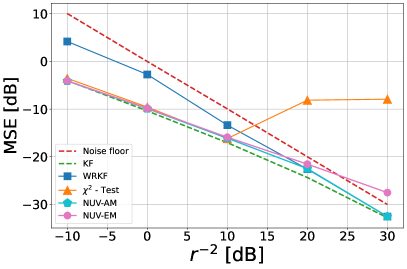
(a) Noisy data clean of outliers

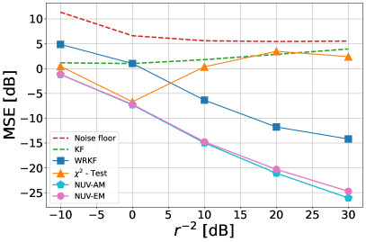
(b) Noisy data with outliers $p=0.2$ $scl=3$

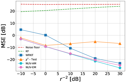
(c) Noisy data with outliers $p=0.2$ $scl=30$

Figure 2: Sub-Fig. 2(a),  2(b) and  2(c) present the mse of the estimated position for the tracking application in the kf setup. Our nuv methods were compared to different well-established robust kf algorithms in the literature.

III-E Discussion

The nuv modeling is particularly efficient due to its sparse features, which can be achieved by selecting the prior distribution of $\boldsymbol{\gamma}^{2}$. To that end, we opt for a uniform prior for the computations’ convenience, which effectively adjusts the overall loss function to accommodate very sparse outliers’ detection. Different choices for this prior would lead to alternative loss functions, such as the convex Huber cost function [7].

To integrate the nuv within the kf, we utilize either the em or am algorithms to estimate the unknown variance of the nuv. The estimated result combines to enhance the kf update step. The main limitation of the em is that it requires the posterior variances of the state $\mathbf{x}_{t}$ in each iteration, which may be infeasible for large problems, while in am version it is obtained from the first-order moment. However, the am proves more effective compared to em, as evident from the empirical evaluation in Section IV.

It is important to note that in certain applications, em empirically gives better results than am, primarily due to its accounting for the accuracy of the state estimate. Its simplicity relies on empirical second-order moments, and holds potential for augmentation with trainable data-driven variations of the kf, for instance [35, 36]. Such fusion leverages robust filtering in partially known ss models and helps manage sensitivity to outliers.

IV Analysis and Results

In this section, we present a comprehensive assessment of the effectiveness of our proposed approaches: oikf based nuv-em, and oikf based nuv-am, for outlier detection within various kf setups. Their performance is evaluated across different outlier intensities and tasks while comparing their effectiveness to other established works in the literature:

1. Simulations: Our first experimental study considers a standard localization task with generated data. The synthetic dataset is generated using the wna (wna) [37] model, and the observation signal is subject to varying degrees of outlier corruption. Such models are commonly used in several applications such as navigation and target tracking.

2. nclt (nclt) Dataset: In our second study, we examine localization use case based on rw data - the Michigan nclt [33] dataset. Here, we compare our methods with different algorithms for tracking rw dynamic data of a moving Segway robot using GNSS noisy measurements.

3. api (api) Dataset: The third and fourth studies involve another localization use case, based on the rw data - the api [34, 43] dataset. Here, we demonstrate the performances of our algorithms in tracking a quadrotor and a marine vessel using GNSS noisy measurements.

IV-A Simulations

In this study, we utilize a kf algorithm where the state vector is represented by,

$$\mathbf{x}=\begin{bmatrix}\mathrm{p}&\mathrm{v}\end{bmatrix}^{\top}$$ (36)

where $\mathrm{p}$ and $\mathrm{v}$ denote the position and velocity states, respectively. For the experiments that involve generated data, we establish the dynamic wna model, followed by a linear ss model. For the filtering process, we assume both position and velocity measurements are available, thus the observation matrix is the identity matrix and the observation noise covariance matrix is diagonal; i.e.,

$$\mathbf{H}=\begin{pmatrix}1&0\\ 0&1\end{pmatrix},\quad\mathbf{R}=\mathrm{r^{2}}\begin{pmatrix}1&0\\ 0&1\end{pmatrix}$$ (37)

The process noise covariance matrix is :

$$\mathbf{Q}=\mathrm{q^{2}}\begin{pmatrix}1&0\\ 0&1\end{pmatrix}$$ (38)

where $\mathrm{q^{2}}$ is the process noise variance, set to a constant value of $-10\left[\textrm{dB}\right]$.

To evaluate our approach, we consider three scenarios for generating measurements: noisy data without outliers, noisy data with mild outliers, and noisy data with significant outliers. The presence of outliers within the measurement vector is modeled with intensities drawn from a Rayleigh distribution with parameter $\sigma{{}_{u}^{2}}$, where we employ two scale parameters $\sigma{{}_{u}^{2}}=\left[3,30\right]$, representing low and high outlier intensities, respectively. The occurrence of outliers in the dataset is determined using a Bernoulli distribution, $\mathcal{B}(p)$, where we set the probability of an outlier to be $p=0.2$, indicating that roughly $20\%$ of the data points are considered outliers. In Figure 2 we compare our proposed oikf based on nuv-em and based on nuv-am with the following algorithms: classical kf, reweighted algorithm (WRKF[15]) and $\chi^{2}$-test [13, 14].

Figure 2(a) presents the results of evaluating the performance of the nuv-am algorithm on synthetic data that is clean of outliers, wherein the algorithm achieves the optimal minimal mse bound by estimating a significant proportion of $\boldsymbol{\gamma}^{2}_{t}$ values as zero. Consequently, the model reverts to the kf. Meanwhile, the $\chi^{2}$-test is deviating significantly from the performance of the kf. This is due to the necessity of determining its confidence level. In cases of low-noise observations, it may incorrectly identify normal samples as outliers, leading to their rejection and rendering the model reliant solely on the prediction step. The relative efficiencies of our oikf and the kf can be assessed based on the resulting mse. Notably, as depicted in Figure 2(a), the average ratio of mse values between the kf and oikf-based nuv-em yields a relative efficiency of $92\%$, while oikf-based nuv-am results in a relative efficiency of $96\%$. This outcome underscores the effectiveness of our algorithms even in the absence of outliers, due to the fact that a Gaussian framework is maintained.

When utilizing synthetic data with outliers, as shown in Figure 2(b) and Figure 2(c) with outlier intensities of $3$ and $30$, respectively, the nuv-am algorithm exhibits superior performance in terms of mse as compared to other algorithms, across varying values of observation noise variance $r^{2}$, and for both high and low outlier intensities. Notably, it demonstrates similar performance to the nuv-em algorithm and even surpasses it for low observation noise without utilizing a second-order moment as in em.

In Figure 3, we exhibit the convergence plots of the estimated variance $\hat{\gamma}^{2}$, using the NUV-am algorithm when an outlier was identified. It is evident that the NUV-AM algorithm achieves rapid convergence after approximately three iterations, regardless of whether the outlier intensities are high or low.

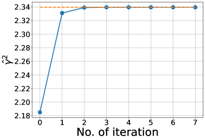
(a) Low outlier intensity

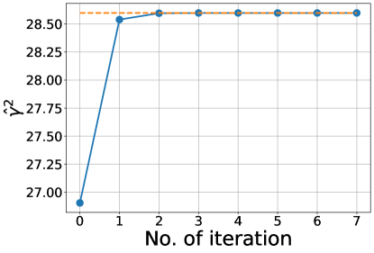
(b) High outlier intensity

Figure 3: Convergence plots of the estimated outliers’ variance computed using the NUV-am algorithm.

IV-B NCLT Dataset

For rw data, we make use of the nclt dataset [33]. The nclt dataset is collected from a session with the date 2013-04-05, which gnss readings sampled at 5[Hz] with a degree of noise and the corresponding ground location information of a Segway robot in motion. To filter out this process, we employ the dynamic wna model [37]. Since only the gnss position is observable in this dataset, the measurement matrix is:

$$\mathbf{H}=\begin{bmatrix}1&0\end{bmatrix},$$ (39)

and the process and measurement noise covariances are

$$\mathbf{R}=\mathrm{r^{2}},\quad\mathbf{Q}=\mathrm{q^{2}}\begin{pmatrix}1&0\\ 0&1\end{pmatrix}$$ (40)

Figure 4 and Figure 5 depict the trajectory of the Segway in the east and north directions, respectively, when the gnss measurements are subjected to outliers, that result in readings deviating significantly from the gt (gt). We have divided each trajectory into two time intervals, with the first interval displaying outliers with lower intensity and the second interval with higher intensity. In addition, Figure 6 present the spatial trajectory of the moving Segway in both directions. In the $x$-axis, we depict the trajectory from Figure 4, while the $y$-axis depicts the trajectory from Figure 5.

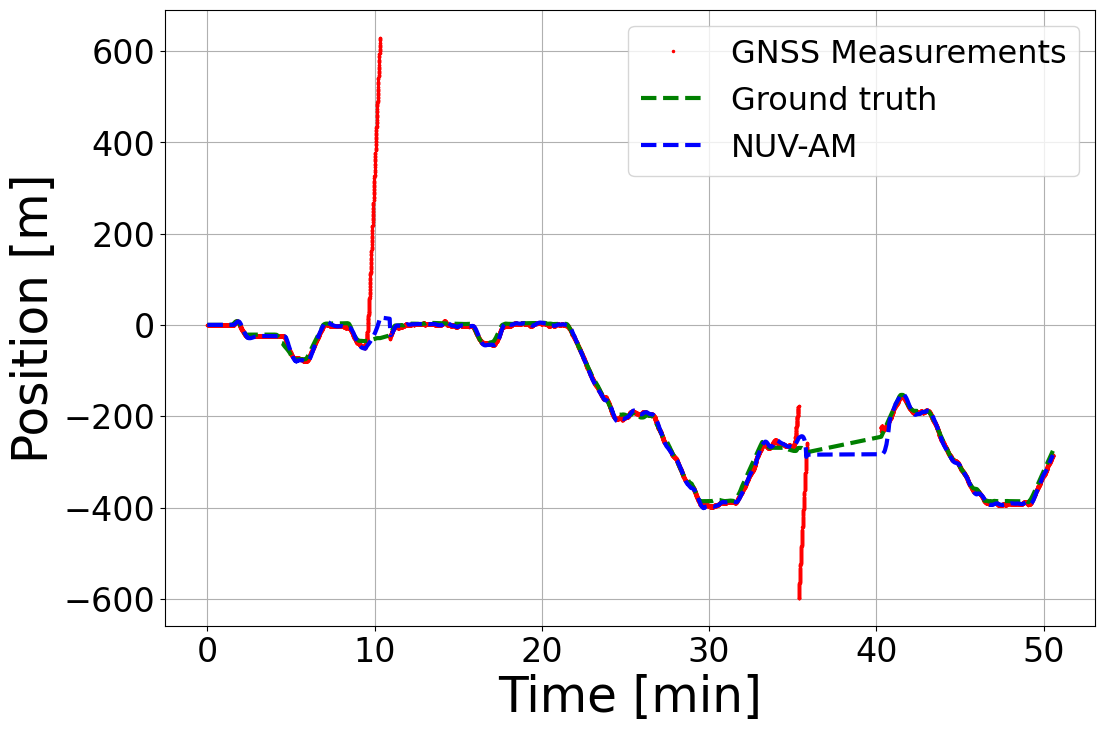
(a) Time interval 0-50[min]

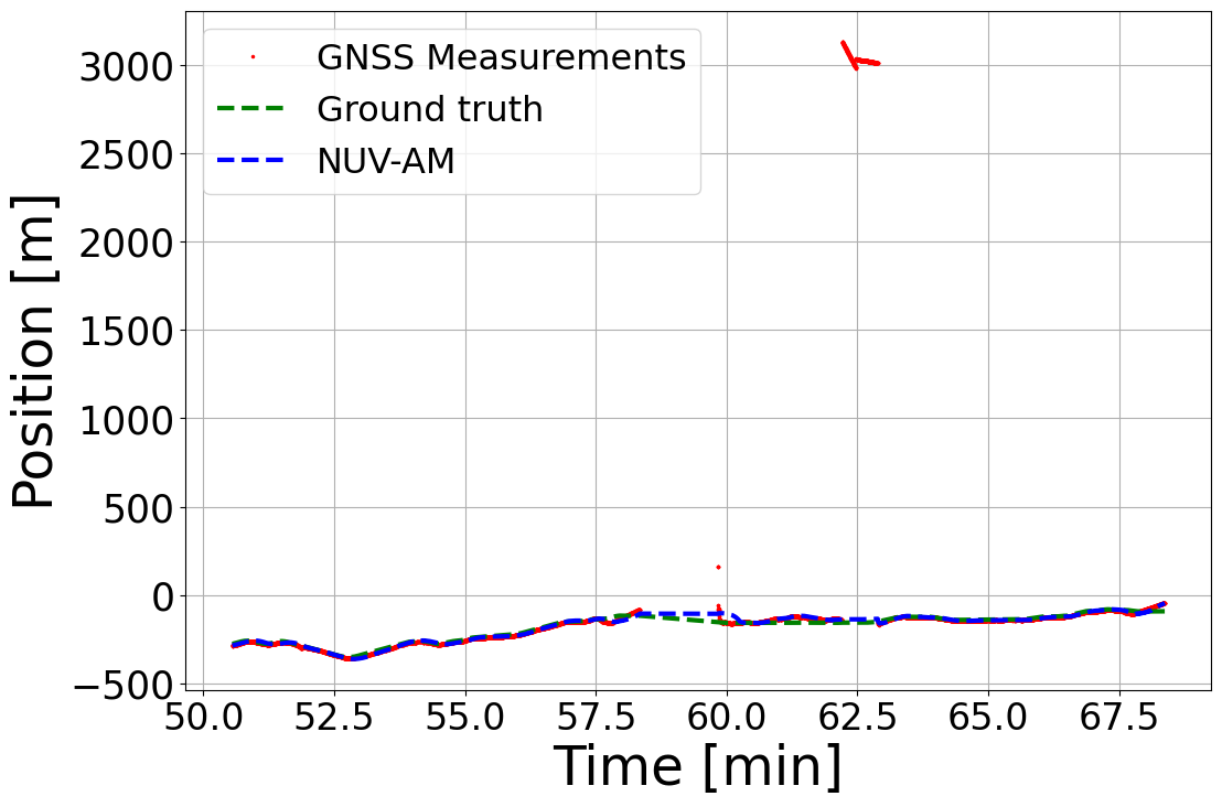
(b) Time interval 50-68[min]

Figure 4: The measured vehicle position in east direction obtained from the noisy gnss nclt dataset (red points), is compared to the estimated trajectory by our nuv-am (blue dashed line), which succeeded in passing the outliers and achieved performance comparable to the ground-truth (green dashed line).

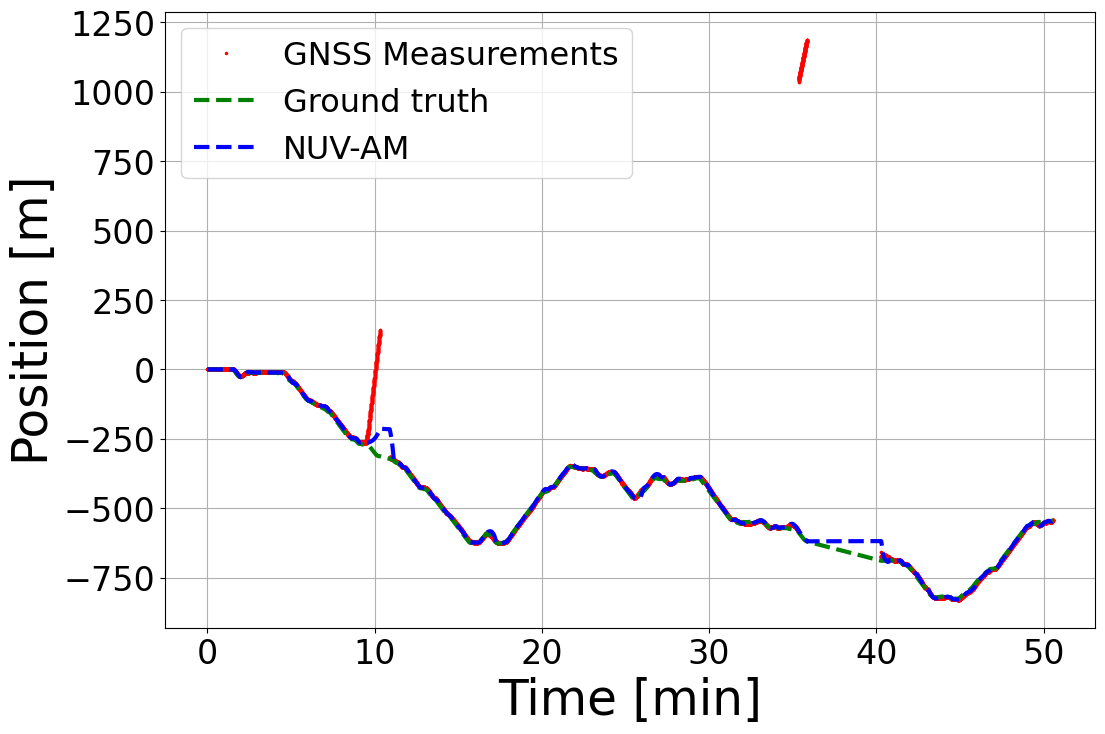
(a) Time interval 0-50[min]

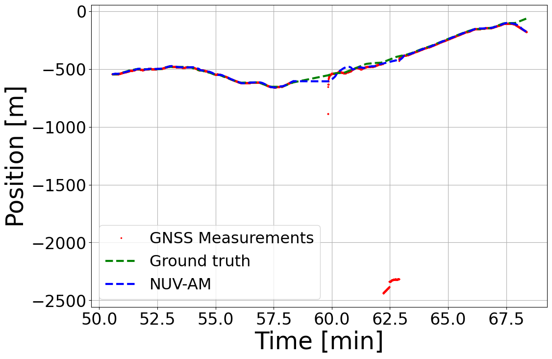
(b) Time interval 50-68[min]

Figure 5: The measured vehicle position in north direction obtained from the noisy gnss nclt dataset (red points), is compared to the estimated trajectory by our nuv-am (blue dashed line), which succeeded in passing the outliers and achieved performance comparable to the ground-truth (green dashed line).

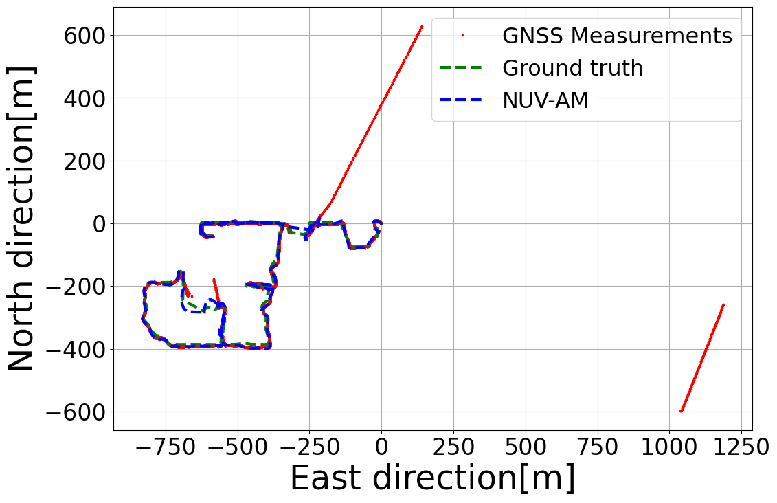
(a) Time interval 0-50[min]

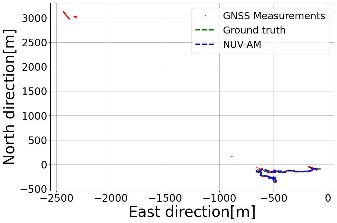
(b) Time interval 50-68[min]

Figure 6: The measured vehicle position structure obtained from the noisy gnss nclt dataset (red points), is compared to the estimated trajectory by our nuv-am (blue dashed line), which succeeded in passing the outliers and achieved performance comparable to the ground-truth (green dashed line).

Our analysis focuses on evaluating the effectiveness of nuv-am in estimating position from real-world data and removing outliers reliably. Table I presents the rmse (rmse) and mse for each algorithm, while the process noise $\mathrm{q}^{2}$ and observation noise variance $\mathrm{r}^{2}$ of each algorithm are optimized separately through grid search to yield the lowest mse. As shown in Table I, oikf with both nuv-em and nuv-am has the lowest estimation errors in both directions, with nuv-am performing slightly better when it coincides with nuv-em, even without utilizing the second-order moment. In terms of computation time, algorithms that combine kf with outlier detection techniques achieve higher accuracy but at the cost of longer computation runtimes, as outlier detection is applied. Compared to other algorithms, the $\chi^{2}$-test stands out as the shortest, stemming from the fact that it only detects and rejects outliers during the prediction step. On the other hand, a more sophisticated technique, such as the ORKF, requires more time due to its increased computational complexity, which requires tuning multiple parameters. Our algorithms present relatively shorter computation times among outlier detection and weighting algorithms, coupled with low MSE, making them suitable for real-time tasks. Additionally, in comparison to our other suggested method, nuv-based em, nuv-based am showcases an almost $40\%$ reduced runtime.

TABLE I: Position error for optimal values of $\mathrm{r}^{2}$ and $\mathrm{q}^{2}$ for nclt dataset

	North direction		East direction		Runtime
	RMSE[m]	MSE$\left[\textrm{dB}\right]$	RMSE[m]	MSE$\left[\textrm{dB}\right]$	[ms]
Noisy GNSS	349.3	50.8	266.1	48.5	-
KF	92.3	39.3	164.4	44.3	0.05
ORKF	27.7	28.8	28	28.9	2.8
ch2t	12.3	21.8	14.2	23	0.1
NUV-AM	10.4	20.3	13	22.3	0.3
NUV-EM	10.3	20.3	13	22.3	0.4

IV-C API Dataset

To emphasize the versatility and robustness of our approaches in tracking rw dynamic data of different platforms, which may be corrupted by various types of outliers, we evaluate the api dataset [34]. The api dataset is collected from the MATRICE 300 quadrotor platform containing gnss RTK reading sampled at $10[Hz]$ and from a marine vessel named ”Shikmona” containing motion reference units (MRU) with gnss RTK receiver, sampled at $100[Hz]$.

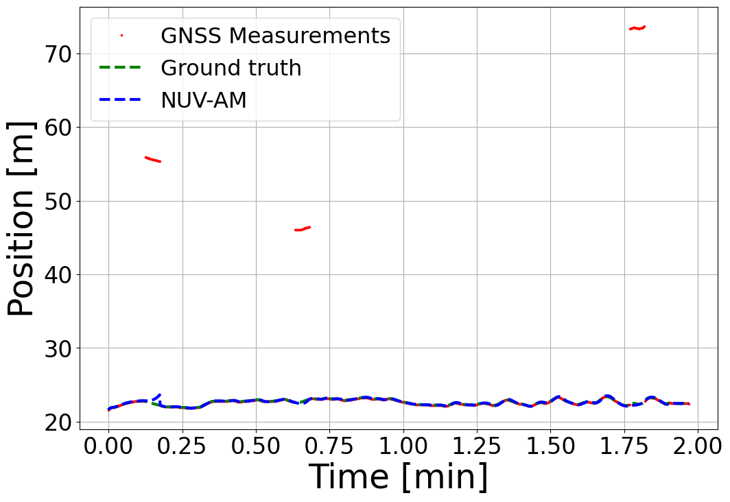
(a) Horizontal direction

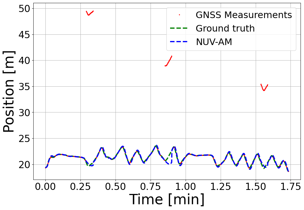
(b) Vertical direction

Figure 7: The measured quadrotor trajectory obtained from the noisy gnss measurements (red points), with the estimated trajectory by our NUV-AM (blue dashed line), and ground-truth (green dashed line).

Their trajectories were populated with generated outliers, sampled with intensity from a Rayleigh distribution, while their time steps within the data were drawn from a Bernoulli distribution. To filter out this process, we use the same model and parameters as in Subsection IV-B.

It is evident from Figure 7 that our oikf based on nuv-am algorithm accurately estimates the position, effectively handling all outliers in both vertical and horizontal directions of the quadrotor trajectory. Table II presents the rmse and mse for each algorithm, while the process noise $\mathrm{q}^{2}$ and observation noise variance $\mathrm{r}^{2}$ of each algorithm are optimized at the same procedure as in the Table I. As shown in Table II, oikf with both nuv-em and nuv-am has the lowest estimation errors for both directions and emphasize the use in nuv method for outlier detection.

TABLE II: Position error for optimal values of $\mathrm{r}^{2}$ and $\mathrm{q}^{2}$ for api dataset - quadrotor recordings.

	Horizontal direction		Vertical direction
	RMSE[m]	MSE$\left[\textrm{dB}\right]$	RMSE[m]	MSE$\left[\textrm{dB}\right]$
Noisy GNSS	10.4	20.3	6.4	16.1
KF	0.9	-1.2	1.8	5.3
ORKF	0.8	-1.9	1	-0.4
ch2t	0.3	-11.4	0.5	-6.3
NUV-AM	0.1	-17.9	0.3	-10
NUV-EM	0.1	-17.9	0.3	-10.2

Figure 8 demonstrates the performance of our oikf-based nuv-am in estimating the position of the ”Shikmona” marine vessel. The examined trajectory including straight line segments and turns. As can be seen, oikf-based nuv-am successfully tracks the ground truth and surpasses outliers, even during turns.Table III underscores our superior performance compared to other algorithms, revealing significantly low rmse and mse values for both our nuv-em and nuv-am algorithms.

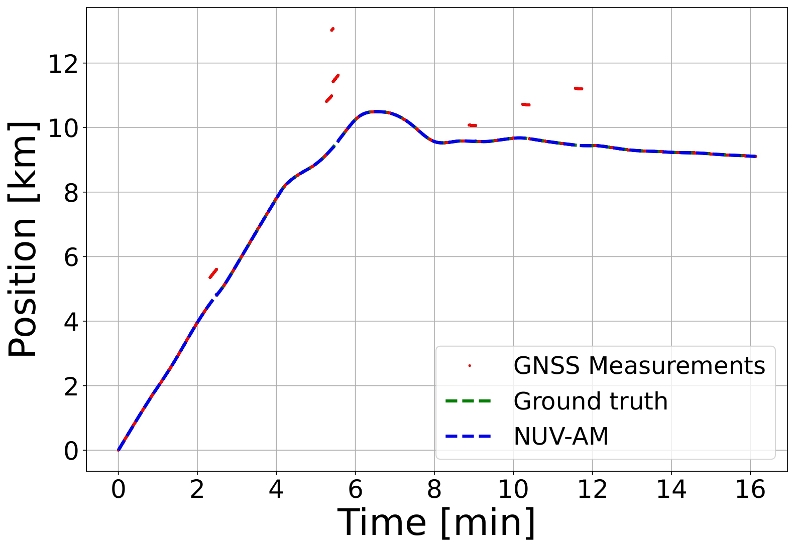
Figure 8: The measured ”Shikmona” marine vessel trajectory obtained from the noisy gnss measurements (red points), with the estimated trajectory by our nuv-am (blue dashed line), and ground-truth (green dashed line).

TABLE III: Position error for optimal values of $\mathrm{r}^{2}$ and $\mathrm{q}^{2}$ for api dataset - marine vessel recordings.

	RMSE[m]	MSE$\left[\textrm{dB}\right]$
Noisy GNSS	373	51
KF	267	48
ORKF	48	34
ch2t	6	16
NUV-AM	2.4	7.52
NUV-EM	2.4	7.52

V Conclusion

In this work, we have proposed an innovative outlier-insensitive kf that offers improved performance to tackle the problem of state estimation in presenence of outliers. Based on Bayesian learning concepts, we model the outlier as nuv and estimate the unknown variance using either em or am algorithms, resulting in sparse outlier detection. Both algorithms are parameter-free and amount essentially to a short iterative process during the update step of the kf. Our numerical study demonstrates the effectiveness of our algorithms and highlights the robustness and wide applicability in addressing a variety of applications. We demonstrate superior performances competing with other algorithms in terms of mse and rmse across synthetic and rw datasets. These findings emphasize the robustness and accuracy of our oikf approach, making it especially suitable for systems reliant on high-quality sensory data.

References

- [1] S. Truzman, G. Revach, N. Shlezinger, and I. Klein, “Outlier-Insensitive Kalman Filtering Using NUV Priors,” IEEE International Conference on Acoustics, Speech and Signal Processing (ICASSP), pp. 1–5, 2023.
- [2] J. Durbin and S. J. Koopman, Time Series Analysis by State Space Methods. Oxford University Press, 05 2012.
- [3] H. Zhu, K. Zou, Y. Li, and H. Leung, “Robust sensor fusion with heavy-tailed noises,” Signal Process., vol. 175, p. 107659, 2020.
- [4] Y. Yuan, Y. Wang, W. Gao, and F. Shen, “Vehicular Relative Positioning With Measurement Outliers and GNSS Outages,” IEEE Sensors Journal, vol. 23, no. 8, pp. 8556–8567, 2023.
- [5] E. Navon and B. Bobrovsky, “An efficient outlier rejection technique for kalman filters,” Signal Process., vol. 188, p. 108164, 2021.
- [6] R. E. Kalman, “A New Approach to Linear Filtering and Prediction Problems,” in Journal of Basic Engineering, 1960, vol. 82, no. 1, pp. 35–45.
- [7] P. J. H. Roncetti and E. M., Robust Statistics, 2nd ed. John Wiley & Sons, 2009.
- [8] S. Farahmand, G. B. Giannakis, and D. Angelosante, “Doubly Robust Smoothing of Dynamical Processes via Outlier Sparsity Constraints,” IEEE Transactions on Signal Processing, vol. 59, no. 10, pp. 4529–4543, 2011.
- [9] A. Y. Aravkin, J. V. Burke, and G. Pillonetto, “Sparse/Robust Estimation and Kalman Smoothing with Nonsmooth Log-Concave Densities: Modeling, Computation, and Theory,” J. Mach. Learn. Res., vol. 14, pp. 2689–2728, 2013.
- [10] J. A. Knight, N.L.;Wang, “A Comparison of Outlier Detection Procedures and Robust Estimation Methods in GPS Positioning,” Journal of Navigation, vol. 62, pp. 699–709, 2009.
- [11] F. Zhu, Z. Hu, W. Liu, and X. Zhang, “Dual-Antenna GNSS Integrated With MEMS for Reliable and Continuous Attitude Determination in Challenged Environments,” IEEE Sensors Journal, vol. 19, no. 9, pp. 3449–3461, 2019.
- [12] N. Ye and Q. Chen, “An anomaly detection technique based on a chi-square statistic for detecting intrusions into information systems,” Quality and Reliability Engineering International, vol. 17, no. 2, pp. 105–112, 2001.
- [13] A. Lekkas, M. Candeloro, and I. Schjølberg, “Outlier rejection in underwater acoustic position measurements based on prediction errorr,” 4th IFAC Workshop on Navigation, Guidance and Control of Underwater Vehicles, vol. 48, no. 2, pp. 82–87, 2015.
- [14] F. Van Wyk, Y. Wang, A. Khojandi, and N. Masoud, “Real-time sensor anomaly detection and identification in automated vehicles,” IEEE Transactions on Intelligent Transportation Systems, vol. 21, no. 3, pp. 1264–1276, 2020.
- [15] J. A. Ting, E. Theodorou, and S. Schaal, “A Kalman Filter for Robust Outlier Detection,” IEEE International Conference on Intelligent Robots and Systems, pp. 1514–1519, 2007.
- [16] G. Agamennoni, J. I. Nieto, and E. M. Nebot, “An Outlier-Robust Kalman Filter,” IEEE International Conference on Robotics and Automation, pp. 1551–1558, 2011.
- [17] Y. Tao and S. S. T. Yau, “Outlier-Robust Iterative Extended Kalman Filtering,” IEEE Signal Processing Letters, vol. 30, pp. 743–747, 2023.
- [18] C. D. Karlgaard and H. Schaub, “Huber-based divided difference filtering,” Journal of guidance, control, and dynamics, vol. 30, no. 3, pp. 885–891, 2007.
- [19] M. A. Gandhi and L. Mili, “Robust Kalman Filter Based on a Generalized Maximum-Likelihood-Type Estimator,” IEEE Transactions on Signal Processing, vol. 58, no. 5, pp. 2509–2520, 2010.
- [20] A. Aravkin, J. V. Burke, L. Ljung, A. Lozano, and G. Pillonetto, “Generalized Kalman Smoothing: Modeling and Algorithms,” Automatica, vol. 86, no. 287381, pp. 63–86, 2017.
- [21] G. Agamennoni, J. I. Nieto, and E. M. Nebot, “Approximate Inference in State-Space Models with Heavy-Tailed Noise,” IEEE Transactions on Signal Processing, vol. 60, no. 10, pp. 5024–5037, 2012.
- [22] Y. Huang, Y. Zhang, N. Li, Z. Wu, and J. A. Chambers, “A Novel Robust Student’s t-based Kalman Filter,” IEEE Transactions on Aerospace and Electronic Systems, vol. 53, no. 3, pp. 1545–1554, 2017.
- [23] N. Davari and A. P. Aguiar, “Real-Time Outlier Detection Applied to a Doppler Velocity Log Sensor Based on Hybrid Autoencoder and Recurrent Neural Network,” IEEE Journal of Oceanic Engineering, vol. 46, no. 4, pp. 1288–1301, 2021.
- [24] F. Wadehn, L. Bruderer, J. Dauwels, V. Sahdeva, H. Yu, and H.-A. Loeliger, “Outlier-insensitive Kalman Smoothing and Marginal Message Passing,” 24th European Signal Processing Conference (EUSIPCO), pp. 1242–1246, 2016.
- [25] M. E. Tipping, “Sparse Bayesian Learning and the Relevance Vector Machine,” J. Mach. Learn. Res., vol. 1, no. 8, pp. 211–244, 2001.
- [26] D. Wipf and B. Rao, “Sparse Bayesian Learning for Basis Selection,” IEEE Transactions on Signal Processing, vol. 52, no. 8, pp. 2153–2164, 2004.
- [27] H.-A. Loeliger, L. Bruderer, H. Malmberg, F. Wadehn, and N. Zalmai, “On Sparsity by NUV-EM, Gaussian Message Passing, and Kalman Smoothing,” Information Theory and Applications Workshop (ITA), pp. 1–10, 2016.
- [28] H.-A. Loeliger, B. Ma, H. Malmberg, and F. Wadehn, “Factor Graphs with NUV Priors and Iteratively Reweighted Descent for Sparse Least Squares and More,” IEEE 10th International Symposium on Turbo Codes & Iterative Information Processing (ISTC), pp. 1–5, 2018.
- [29] H.-A. Loeliger, “On NUV priors and Gaussian message passing,” IEEE International Workshop on Machine Learning for Signal Processing (MLSP), 2023.
- [30] A. P. Dempster, N. M. Laird, and D. B. Rubin, “Maximum Likelihood from Incomplete Data Via the EM Algorithm,” Journal of the Royal Statistical Society: Series B, vol. 39, no. 1, pp. 1–22, 1977.
- [31] J. A. Palmer, D. P. Wipf, K. Kreutz-Delgado, and B. D. Rao, “Variational em algorithms for non-gaussian latent variable models,” in Advances in neural information processing systems, 2005, pp. 1059–1066.
- [32] V. S. A Andresen, “Convergence of an Alternating Maximization Procedure,” Journal of Machine Learning Research, vol. 17, 2016.
- [33] N. Carlevaris-Bianco, A. K. Ushani, and R. M. Eustice, “University of Michigan North Campus long-term vision and lidar dataset,” International Journal of Robotics Research, vol. 35, no. 9, pp. 1023–1035, 2016.
- [34] A. Shurin, A. Saraev, M. Yona, Y. Gutnik, S. Faber, A. Etzion, and I. Klein, “The Autonomous Platforms Inertial Dataset,” IEEE Access, vol. 10, pp. 10 191–10 201, 2022.
- [35] G. Revach, N. Shlezinger, X. Ni, A. L. Escoriza, R. J. G. van Sloun, and Y. C. Eldar, “KalmanNet: Neural Network Aided Kalman Filtering for Partially Known Dynamics,” IEEE Transactions on Signal Processing, vol. 70, pp. 1532–1547, 2022.
- [36] G. Revach, X. Ni, N. Shlezinger, R. J. G. van Sloun, and Y. C. Eldar, “RTSNet: Learning to Smooth in Partially Known State-Space Models,” IEEE Transactions on Signal Processing, vol. 71, no. 1, pp. 4441–4456, 2023.
- [37] Y. Bar-Shalom, X. R. Li, and T. Kirubarajan, Estimation with applications to tracking and navigation: Theory algorithms and software. John Wiley & Sons, 2004.
- [38] H. Ohlsson, F. Gustafsson, L. Ljung, and S. P. Boyd, “Smoothed state estimates under abrupt changes using sum-of-norms regularization,” Autom., vol. 48, no. 4, pp. 595–605, 2012.
- [39] B. Bell and F. Cathey, “The Iterated Kalman Filter Update as a Gauss-Newton Method,” IEEE Transactions on Automatic Control, vol. 38, no. 2, pp. 294–297, 1993.
- [40] J. Humpherys, P. Redd, and J. M. West, “A Fresh Look at the Kalman Filter,” SIAM Rev., vol. 54, no. 4, pp. 801–823, 2012.
- [41] B. Ma, N. Zalmai, R. Torfason, C. Striti, and H.-A. Loeliger, “Color image segmentation using iterative edge cutting, NUV-EM, and Gaussian message passing,” IEEE Global Conference on Signal and Information Processing (GlobalSIP), pp. 161–165, 2017.
- [42] P. J. Rousseeuw and M. Hubert, “Robust Statistics for Outlier Detection,” WIREs Data Mining Knowl. Discov., vol. 1, no. 1, pp. 73–79, 2011.
- [43] A. Shurin and I. Klein, “QuadNet: A Hybrid Framework for Quadrotor Dead Reckoning,” Sensors, vol. 22, no. 4, p. 1426, 2022.