PromptST: Prompt-Enhanced Spatio-Temporal Multi-Attribute Prediction
Abstract.
In the era of information explosion, spatio-temporal data mining serves as a critical part of urban management. Considering the various fields demanding attention, e.g., traffic state, human activity, and social event, predicting multiple spatio-temporal attributes simultaneously can alleviate regulatory pressure and foster smart city construction. However, current research can not handle the spatio-temporal multi-attribute prediction well due to the complex relationships between diverse attributes. The key challenge lies in how to address the common spatio-temporal patterns while tackling their distinctions. In this paper, we propose an effective solution for spatio-temporal multi-attribute prediction, PromptST. We devise a spatio-temporal transformer and a parameter-sharing training scheme to address the common knowledge among different spatio-temporal attributes. Then, we elaborate a spatio-temporal prompt tuning strategy to fit the specific attributes in a lightweight manner. Through the pretrain and prompt tuning phases, our PromptST is able to enhance the specific spatio-temoral characteristic capture by prompting the backbone model to fit the specific target attribute while maintaining the learned common knowledge. Extensive experiments on real-world datasets verify that our PromptST attains state-of-the-art performance. Furthermore, we also prove PromptST owns good transferability on unseen spatio-temporal attributes, which brings promising application potential in urban computing. The implementation code is available to ease reproducibility111https://github.com/Zhang-Zijian/PromptST.
1. Introduction
Fast urbanization has brought unprecedented convenience to our lives, and also facilitated explosively growth in transportation, security incidents, social events etc. However, it pressures the authority to keep a watchful eye on all these issues (Liu and Li, 2020), which requires burdensome expert efforts and economic costs. Thanks to the prosperous development of Spatio-Temporal Data Mining (STDM), it has become a reality to analyze urban big data and predict future trends (Tascikaraoglu, 2018), e.g., intelligent transportation systems (Zhang et al., 2017; Han et al., 2023; Wang et al., 2021), weather and air quality prediction (Han et al., 2021b; Zhao et al., 2017), and crime prediction (Zhao et al., 2022; Zhao and Tang, 2017a, 2018, b; Zhao et al., 2016a).
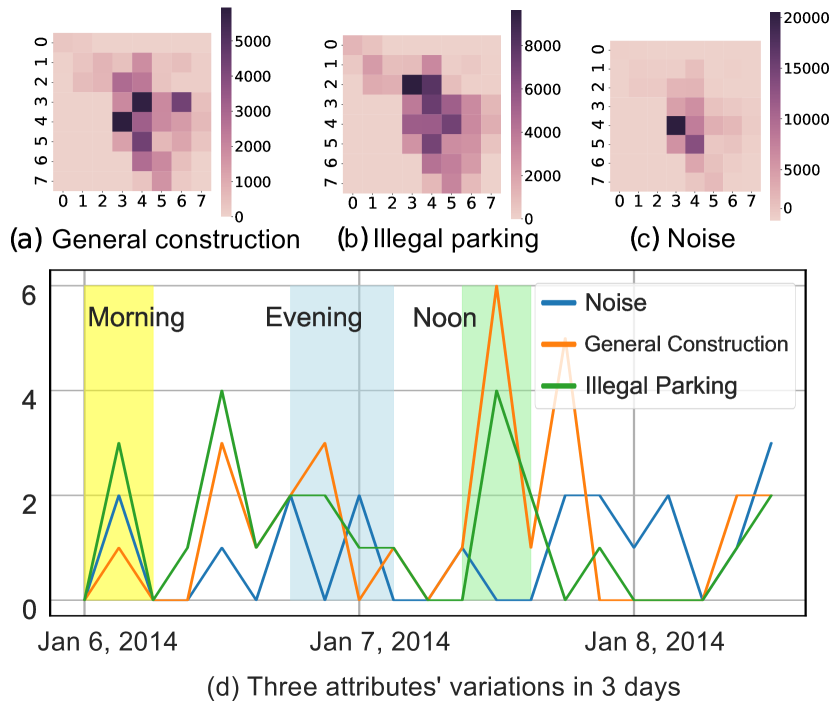
The miscellaneous tasks required to be handled in city management emerge in complex spatio-temporal patterns. Considering the function of different regions, human activities in different regions proceed in similar or different ways. Take regional complaint records from NYC 311222https://portal.311.nyc.gov/ as an example, Figure 1 (a), (b), and (c) illustrate the complaints for ‘general construction’, ‘illegal parking’, and ‘noise’, respectively. Figure 1 (a) and (b) share similar spatial patterns because building and parking problems generally arise in the city. In contrast, (c) owns a prominent high volume in grid , which can be ascribed to the high human mobility in the downtown area. Besides, we also find that different attributes change in similar or different trends over time. Figure 1 (d) shows the three attributes’ variations in three days. The three types of complaints all occur in the morning, but complaints of noise are reported more in the evening and the other two peak at noon. These multiple spatio-temporal attributes are intertwined, and analyzing and utilizing their correlations is of great significance for spatio-temporal multi-attribute prediction and unifying smart city management.
Currently, existing STDM works can not handle the spatio-temporal multi-attribute prediction well. Spatio-temporal prediction methods generally focus on higher performance on a single attribute (Yu et al., 2017; Zheng et al., 2020), which integrates expert knowledge-based inductive bias (Wang et al., 2021; Zhang et al., 2020b) and devises highly-specific architectures for single tasks. For example, STGCN (Yu et al., 2017) utilizes the ChebNet graph convolution to predict traffic flows. GMAN (Zheng et al., 2020) proposes a fabricated model equipped with an attention mechanism to forecast traffic volume or traffic speed. This line of work ignores the relationship between multiple spatio-temporal attributes and fails to address multi-attribute prediction. On the other hand, Spatio-temporal multi-task learning methods pay attention to solving two specific tasks with similar spatio-temporal patterns, which is hard to be extended to numerous tasks due to the highly specified architecture. For instance, MDL (Zhang et al., 2019) and pmlLSTM (Zhang et al., 2020b) are the representative attempts predicting two traffic flows simultaneously, where the convolutional neural networks and LSTM are incorporated, respectively. GEML (Wang et al., 2019) and MT-ASTN (Wang et al., 2020) propose to handle traffic flow and on-demand flow, where the challenge is the feature fusion of different shapes. Recently, AutoSTL (Zhang et al., 2023) shows promising capability on multiple spatio-temporal tasks. However, it also focuses on two tasks, leaving performance on numerous attributes unexplored.
To shed light on the solution of spatio-temporal multi-attribute prediction, we recognize three properties that a spatio-temporal multi-attribute approach should own: (i) Generality. To model the numerous spatio-temporal attributes, the model should well-capture the common characteristics among various attributes. (ii) Adaptivity. Facing diverse spatio-temporal patterns, the model is supposed to be flexible to fit distinct characteristics of the specific attributes. (iii) Transferability. Considering the extensive application scenarios of spatio-temporal prediction, the method is supposed to be lightweight and easily extensible to new tasks.
To accomplish the goals above, challenges in three aspects should be conquered. (i) Capturing the common characteristic among multiple attributes demands high capacity and effective spatio-temporal modeling. (ii) The model should address the specific attributes well while maintaining common knowledge. (iii) The model is supposed to have advancing time and space efficiency so as to be deployed generally. Large pretrain models (Brown et al., 2020a) seem to be a potential solution, which can enhance the performance on target attributes based on the common knowledge learned from large datasets. However, while showing effectiveness over related tasks (Aghajanyan et al., 2021; Shao et al., 2022), such pretrain and fine-tune pattern suffers from the large retraining cost and catastrophic forgetting (Ramasesh et al., 2021; McCloskey and Cohen, 1989).
In this paper, we propose a pretrain and prompt tuning method, PromptST, to solve spatio-temporal multi-attribute prediction effectively. We first put forward an effective spatio-temporal transformer and train it with multiple spatio-temporal attributes in a parameter-sharing manner. Thus, it can well-address the common knowledge of multiple spatio-temporal attributes. We devise novel spatio-temporal prompt tokens and insert them into the feature sequence during target attribute tuning (Gao et al., 2021; Liu et al., 2023). By fixing the main body of pretrained transformer and only tuning prompt tokens with head, our PromptST achieves a good balance between fitting the target spatio-temporal attribute and maintaining the common spatio-temporal knowledge. Common spatio-temporal knowledge can also enhance the modeling of new tasks with lightweight tuning, thus facilitating the analysis of urban attributes in more domains. Our method attains state-of-the-art performance on two real-world datasets (with 19 and 4 different physical tasks respectively) by only tuning 11% of the backbone model parameters. Besides, we explore a lightweight version of prompt tuning, tiny spatio-temporal prompt, to further improve the time and space efficiency, which demands trivial (less than 1% of model parameters) trainable parameters. Our PromptST also shows good transferability to fit the unseen spatio-temporal attributes. In a nutshell, our main contributions are as follows:
-
•
For the first time, we propose a pretrain-prompt tuning scheme, PromptST, to solve the spatio-temporal multi-attribute prediction. It can well fit the specific spatio-temporal pattern of multiple attributes with the enhancement of learned common knowledge;
-
•
Our lightweight spatio-temporal prompt tokens save almost 89% trainable parameters in the tuning phase, with its tiny version achieving a reduction of 99%. This immensely motivates the wide deployment of urban attribute analyzers;
-
•
Extensive experiments on two real-world datasets verify the state-of-the-art performance of PromptST against diverse advancing baselines. Furthermore, PromptST also possesses good transferability, which solves unseen attributes with trivial training costs and shows promising potential for real-world applications.
2. Preliminary
Spatio-Temporal Multi-Attribute Prediction. Let represent the spatio-temporal attribute of historical timesteps and regions. Given historical spatio-temporal attributes, spatio-temporal multi-attribute prediction aims to predict attributes of the future timesteps simultaneously. Mathematically, the prediction could be formulated as follows,
| (1) |
where parameterized by represents the trainable model. denotes the spatio-temporal attribute of future timesteps. For a clear description, we denote with , and let represent the observed spatio-temporal attributes. Let represent the future spatio-temporal attributes of timesteps.
3. Methodology
Extensive efforts have been exerted in spatio-temporal prediction of a single attribute (Wu et al., 2019; Zhang et al., 2017, 2020a). However, these methods cannot well address spatio-temporal multi-attribute prediction: Simply expanding the feature dimension to support multi-attribute ignores and cannot utilize the correlation among different attributes. Training on multiple attributes separately requires tremendous computational and storage costs, which is impractical in application.
In this section, we present a pretrain-prompt tuning scheme to address spatio-temporal multi-attribute prediction, named PromptST. We first propose our benchmark architecture spatio-temporal transformer, and then introduce the pretrain and prompt tuning phases, respectively. We detail our novel spatio-temporal prompt tokens, which fit the specific attributes with trivial trainable parameters.
3.1. Framework Overview
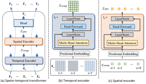
We first propose an effective transformer-based architecture to capture common knowledge of multiple spatio-temporal attributes. As shown in Figure 2 (a), from bottom to top, our transformer architecture consists of temporal encoder, spatial encoder, and head. To balance the model training on multiple attributes, we feed the transformer with single spatio-temporal attributes in parallel which share the model parameters. The temporal encoder and spatial encoder are illustrated in Figure 2 (b) and (c), respectively.
In the pretrain phase, we train the architecture in a parameter-sharing way so that the model learns the common spatio-temporal characteristics among all attributes. To enhance the performance on specific spatio-temporal attributes, we propose a prompt tuning phase to fit each attribute, which benefits the specific attribute modeling from the learned common spatio-temporal patterns. Specifically, by fixing the main body of the pretrained framework, i.e., temporal encoder and spatial encoder, and only updating the prompt tokens and head, our PromptST can capture the specific spatial and temporal patterns of every single attribute with trivial trainable parameters. In this way, our method can address common spatio-temporal characteristics shared among all spatio-temporal attributes, and fits specific ones in a parameter-efficient way.
3.2. Spatio-Temporal Transformer
Due to the superior capacity in related tasks (Vaswani et al., 2017; Zhou et al., 2021), transformer has been introduced in spatio-temporal prediction (Yan et al., 2021; Lan et al., 2022; Guo et al., 2021b; Chen et al., 2022). However, there is still a lack of a solution for spatio-temporal multi-attribute prediction, which can address the complex relationships among numerous attributes effectively. In this section, we propose a swift transformer-based backbone which enjoys a compact architecture and compelling efficacy in modeling spatio-temporal dependency of multiple attributes.
3.2.1. Temporal Encoder
Temporal dependency capture plays a prominent role in spatio-temporal prediction. In general, our temporal encoder consists of a stacked multi-head attention block and a position-wise feed-forward layer.
Positional Embedding. In particular, we first employ an MLP-based mapping function to learn the embedding of each input spatio-temporal attribute as . To learn the temporal information, we transpose the dimension of region and timestep of , i.e., from to , so the mapping operation is,
| (2) |
where and are learnable weight and bias, respectively. is the learned representation, and is the embedding size. and are sigmoid and transpose functions, respectively.
To integrate sequential information into the transformer, we utilize trainable positional embedding to mark the temporal sequence. Specifically, we add positional embedding to ,
| (3) |
Multi-Head Attention. The self-attention mechanism (Vaswani et al., 2017) is the key component of transformer, it calculates the self-attention based on scaled dot-product, and outputs the attention-weighted sum of the feature. The self-attention calculation is shown as follows,
| (4) |
where , , and are the query, key, and value matrix, respectively.
The multi-head attention splits the input feature into several partitions, and conducts self-attention individually. Hence, the feature could be handled in different embedding subspaces, and then concatenated to integrate diverse information,
| (5) | ||||
where , , and are learnable parameter matrices.
Equipped with residual connection (He et al., 2016) and layer normalization (Ba et al., 2016), the multi-head attention operation is conducted as,
| (6) |
Feed-Forward Layer. Then, position-wise feed-forward is applied to each position separately, which is followed by residual connection and layer normalization,
| (7) | ||||
where , are parameter matrices, and , are biases.
Based on Eq. (6) and (7), the temporal intermediate representation after the -th iteration can be calculated as,
| (8) |
We conduct temporal encoder layers of multi-head attention and feed-forward layer to capture the temporal dependency. Then, we take the intermediate representation of the last timestep as the temporal representation of ,
| (9) |
3.2.2. Spatial Encoder
After capturing the temporal dependency with temporal encoder, we address the spatial relationship among the grids. Without extra computational cost such as k-hop adjacency matrix (Yan et al., 2021; Lan et al., 2022), we incorporate a simple but effective spatial encoder to learn spatial information. Generally, we add spatial positional information, and process with stacked multi-head attention and feed-forward layer.
Positional Embedding. Similar to Eq. (3), given temporal representation , we add learnable positional embedding to learn the positional information among the grids.
| (10) |
Spatial Representation Learning. The spatial encoder consists of stacked multi-head attention and feed-forward layer , as shown in Eq. (6) and (7). The spatial intermediate representation output by the -th iteration is,
| (11) |
Processed by layers of multi-head attention and feed-forward layer as spatial encoder, the spatial representation is the output of the spatial encoder,
| (12) |
3.2.3. Head
To map the learned spatio-temporal representation to the future timesteps, we introduce an MLP-based head for the dimension transformation. The predicted spatio-temporal attribute ’s future State can be calculated as,
| (13) |
where and are weight matrix and bias.
3.3. Pretrain Phase
To address the common characteristics among multiple spatio-temporal attributes, we devise a parameter-sharing training strategy (Wang et al., 2022; Brown et al., 2020b; Yan et al., 2022). In this pretrain phase, we train the spatio-temporal transformer with all the spatio-temporal attributes. Specifically, we feed attributes in parallel, which share the same parameters as shown in Figure 2 (a).
Given the spatio-temporal attributes matrix , we feed spatio-temporal transformer with single spatio-temporal attribute matrix with simultaneously. For the output , we concatenate attributes as .
We denote the model parameters of temporal encoder and spatial encoder as , the parameters of head as , and the sum of the two constitute the spatio-temporal transformer.
The optimization objective of pretrain could be formulated as,
| (14) | ||||
where the model output .
3.4. Prompt Tuning Phase
Given the diverse attributes to be tackled in smart city construction, it demands a swift training strategy to save the training and deployment costs as much as possible. In this section, we propose a pretrain-prompt tuning pattern to alleviate the heavy training cost while achieving better performance. We present spatio-temporal prompt and by prompt tuning with it, we can well-fit the specific spatio-temporal pattern of each spatio-temporal attribute with trivial trainable parameters.
3.4.1. Spatio-Temporal Prompt
During the pretrain phase, we obtain common spatio-temporal characteristics in . To enhance the approximation of each attribute, a straightforward solution is fine-tuning (Sun et al., 2019), which loads and re-trains the whole model on single attributes. However, pretrain fine-tuning pattern demands tremendous computational costs for tuning all backbone parameters, and suffers from catastrophic forgetting (Ramasesh et al., 2021; McCloskey and Cohen, 1989).
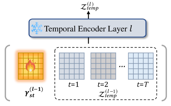
To prompt the pretrained model with specific spatio-temporal attributes, we propose a novel spatio-temporal prompt token into the input sequence. We build trainable spatio-temporal prompt tokens with the same shape of intermediate temporal features, i.e., . Then, we insert prompt tokens to the feature sequence of each layer of the temporal encoder so as to trigger the learned common spatio-temporal pattern in .
Through trainable prompt tokens and optimizing with backbone tuning, this prompt tuning strategy is able to enhance the performance of the specific attributes based on the maintained common knowledge. The spatio-temporal prompt tuning process is shown in Figure 3.
Specifically, we integrate learnable spatio-temporal prompt tokens to the input temporal representation of each layer on the temporal dimension. Hence, the dimension of the concatenated temporal representation is . After processing with multi-head attention and feed-forward layer, we truncate the added to keep the original sequence length, and the truncated . So the temporal intermediate representation in Eq. (8) becomes as,
| (15) |
3.4.2. Prompt Tuning
Recently, prompt learning has shown its effects in triggering the common knowledge maintained in the pretrained backbone (Petroni et al., 2019; Brown et al., 2020b) and enhancing the target task performance. It integrates lightweight prompt tokens in the input sequence and tunes the pretrained backbone to prompt the backbone with the specific information of the target task. However, in spatio-temporal prediction, we need to prompt the backbone with the target task’s temporal and spatial information, which is intricate to be defined compactly. In this context, we elaborate trainable spatio-temporal prompt tokens, to indicate both spatial and temporal properties of target attributes.
Given the pretrained , rather than tuning the whole backbone parameters like fine-tuning, the prompt tuning phase aims to tune a small part of the spatio-temporal transformer, i.e., . Specifically, we load , freeze the , and initialize the and prompt token for each spatio-temporal attribute. Mathematically, the optimizing process is,
| (16) | ||||
where the model output .
3.4.3. Discussion
To comprehensively exhibit our prompt tuning strategy, we discuss several aspects in this section.
Prompting Spatial and Temporal Information. Prompt tuning aims to prompt the backbone with the target task’s information by refined prompt tokens (Brown et al., 2020b; Petroni et al., 2019). It is noteworthy that by adding to each temporal encoder layer, our PromptST is able to capture the characteristic at both spatial and temporal level. Specifically, the spatio-temporal prompt tokens prompt the spatio-temporal transformer for the temporal information of downstream attribute. Besides, each spatio-temporal prompt consists of tokens, which address the spatial information of each region. So tuning spatio-temporal prompt tokens is able to maintain both spatial and temporal characteristics of the target attribute and prompt the backbone.
Space Efficiency. For layers in temporal encoder, we iteratively integrate and truncate the spatio-temporal prompt tokens, so the total spatio-temporal prompt tokens are . For example, given a common setting with and , owns 8,192 parameters. Adding the head , prompt tuning of spatio-temporal prompt trains 8,588 parameters, which is 11.17% of the whole transformer. That means, compared with fine tuning all backbone parameters, our PromptST reduces almost 89% trainable parameters when tuning on target attributes. Considering the numerous spatio-temporal attributes, one can pretrain the backbone once and prompt tune everywhere efficiently.
PromptST v.s. Existing Prompt Tuning Methods. Compared with the existing prompt learning methods in NLP (Brown et al., 2020b; Petroni et al., 2019; Li and Liang, 2021; Gao et al., 2021) and CV (Jia et al., 2022; Wang et al., 2022), our technical contributions lie in two aspects. We propose a novel backbone, i.e., spatio-temporal transformer, and a corresponding pretrain strategy to address the common spatio-temporal pattern in multiple attributes. Besides, we devise a novel spatio-temporal prompt tuning strategy to indicate both spatial and temporal characteristics of target single attributes efficiently.
| Dataset | Complaint | NYC Taxi | Parameter | |||
| Metrics | RMSE | MAE | RMSE | MAE | ||
| (a) | Conv-GCN | 1.6987 0.0332 | 0.3205 0.0076 | 38.9876 0.0017 | 18.0373 0.0025 | 848,960 |
| HGCN | 1.5489 0.0203 | 0.2945 0.0047 | 22.6791 0.3155 | 10.3204 0.1961 | 593,307 | |
| ASTGCN | 1.4022 0.0018 | 0.2559 0.0002 | 16.3039 0.3518 | 7.4875 0.1346 | 73,906 | |
| GWNet | 1.4426 0.0075 | 0.2617 0.0021 | 16.3151 0.2104 | 7.2020 0.0644 | 537,484 | |
| CCRNN | 1.7502 0.0179 | 0.4609 0.0398 | 62.3831 4.9698 | 38.0159 4.3689 | 292,855 | |
| GTS | 1.5902 0.0037 | 0.2808 0.0029 | 19.2680 0.7675 | 8.4905 0.0162 | 9,400,723 | |
| TrafficTmr | 1.7356 0.0003 | 0.3210 0.0010 | 60.6256 3.8161 | 29.4076 2.3559 | 220,108 | |
| (b) | ASTGCN-Full | 1.7569 0.0014 | 0.5536 0.0002 | 54.8019 0.2570 | 33.5280 0.1283 | 91,150 |
| GWNet-Full | 1.7489 0.0087 | 0.3397 0.0045 | 31.3766 0.2506 | 13.9877 0.2057 | 538,636 | |
| CCRNN-Full | 2.0607 0.5015 | 0.8617 0.5339 | 64.2304 10.7221 | 41.8823 9.0472 | 315,373 | |
| TrafficTmr-Full | 1.8333 0.0036 | 0.6158 0.0074 | 67.5295 1.7047 | 41.4542 2.3701 | 227,812 | |
| DMSTGCN | 1.7585 0.0002 | 0.3274 0.0014 | 30.8563 0.6408 | 14.0257 0.1979 | 630,468 | |
| (ours) | Single-Train | 1.4730 0.0004 | 0.2863 0.0006 | 14.4828 0.0689 | 6.8693 0.8456 | 76,876 |
| Full-Train | 1.1673 0.0124 | 0.3109 0.0070 | 15.2143 0.1999 | 7.0856 0.1173 | 76,876 | |
| Fine-Tune | 1.2362 0.0101 | 0.2653 0.0016 | 14.5352 0.0238 | 6.7474 0.0285 | 76,876 | |
| PromptST | 1.1189* 0.0027 | 0.2432* 0.0054 | 14.2907* 0.0738 | 6.6882* 0.0251 | 8,588 | |
4. Experiment
In this section, we comprehensively verify the efficacy of PromptST against advancing baselines. We conduct further transferability experiments to investigate the potential on unseen spatio-temporal attributes. Besides, we devise ablation study and hyper-parameter analysis to verify the contribution of key components. We also present the time and space efficiency comparison, which further emphasizes the efficacy and effectiveness of our PromptST.
4.1. Datasets
We eavluate PromptST on two physical spatio-temporal multi-attribute datasets: Complaint333https://opendata.cityofnewyork.us/ and NYC Taxi444https://www1.nyc.gov/site/tlc/about/tlc-trip-record-data.page. The datasets are split into training, validation, and test sets by the ratio of 7:1:2.
Complaint. The NYC 311 service offers assistance to requests, and record the 216 types of complaint with corresponding location and time. We collect records of 19 kinds of complaints with the largest volumes in 2013 and 2014 as dataset Complaint, including 2.27M complaints about noise, dirty conditions, traffic signal condition, illegal parking, etc.
NYC Taxi. NYC Taxi datasets record taxi trajectories in New York City. Each trajectory consists of trip information, including fare, number of passengers, start and arrival time and corresponding geological properties. To describe the timely flows of vehicles and passengers, We compute the traffic inflow, traffic outflow, population inflow, and population outflow between city regions as spatio-temporal attributes.
4.2. Baselines
We compare our PromptST with the advancing baselines from three lines: (a) Spatio-temporal prediction: Train models on each single attribute individually. Conv-GCN (Zhang et al., 2020a), HGCN (Guo et al., 2021a), ASTGCN (Guo et al., 2019a), GWNet (Wu et al., 2019), CCRNN (Ye et al., 2021), GTS (Shang and Chen, 2021), and TrafficTmr (Yan et al., 2021). (b) Spatio-temporal multi-attribute prediction: Expand feature dimension to multiple attributes and train a single model on multiple attributes. ASTGCN-Full,GWNet-Full,CCRNN-Full,TrafficTmr-Full,and DMSTGCN (Han et al., 2021a). (ours) Our spatio-temporal transformer in three training strategies: Single-Train: train spatio-temporal transformer on each attribute individually, Full-Train: train spatio-temporal transformer on all attributes, and Fine-Tune: tune full-trained model on each attribute individually.
4.3. Experiment Setups
We predict the spatio-temporal attributes of future 12 timesteps based on historical 12 timesteps, i.e., . To evaluate the model capacity, we use root mean squared error (RMSE) and mean absolute error (MAE) as evaluation metrics. We incorporate two layers for the temporal encoder and spatial encoder for the spatio-temporal transformer, respectively, i.e., . We integrate prompt tokens in the tuning phase. We use Adam as optimizer with a learning rate of 0.003 and a hidden size of 32. All experiments are conducted on one NVIDIA 2080-Ti GPU, and we compute the average result of 5 repetitions for all the results.
4.4. Overall Performance
According to the experimental results in Table 1, we can safely draw conclusions below,
(1) The advancing spatio-temporal prediction methods, i.e., GraphWaveNet, CCRNN and MTGNN, achieve poor results on spatio-temporal multi-attribute prediction. Upgrading the feature dimension to fit multiple attributes can not handle the entangled spatio-temporal patterns among different attributes. Hence, the multi-attribute version of the two performs worse than the single-training ones, where the latter runs on each attribute repetitively. (2) The full-trained spatio-temporal transformer achieves a remarkably leading position against all the baselines, with a relatively small parameter scale. This verifies the compact and effective architecture of our spatio-temporal transformer and the efficacy of the parameter-sharing training strategy towards spatio-temporal multi-attribute prediction. (3) Single-Train achieves comparable results with Full-Train, which is in accordance with the expectation because in Single-Train the spatio-temporal transformer can well-fit the specific pattern of each attribute. However, the Full-Train defeats Single-Train in some scenarios, i.e., RMSE of 1.1673 v.s. 1.4730 on Complaint. This indicates that there exists common spatio-temporal knowledge among different attributes, and well-exploiting the common pattern contributes to spatio-temporal prediction. (4) According to the performance of Fine-Tune and Full-Train, fine-tuned transformer generally exceeds the full-trained one, except for the RMSE on Complaint. It could be ascribed to the catastrophic forgetting (Ramasesh et al., 2021; McCloskey and Cohen, 1989), which erases the common spatio-temporal knowledge learned in the pretrained model and degenerates to fitting the spatio-temporal pattern of the single attribute as Single-Train. (5) We can observe a consistent improvement of PromptST beyond the fine-tuned result on all metrics of both datasets with about 10% parameters tuned. Specifically, PromptST achieves better RMSE results on 14 out of 19 spatio-temporal attributes in Complaint, RMSE results on 3 out of 4 spatio-temporal attributes in NYC Taxi. Our prompt tuning strategy alleviates the catastrophic forgetting phenomenon and well-fits the specific characteristic of the target spatio-temporal attribute.
Hence, our PromptST achieves promising performance on spatio-temporal multi-attribute prediction. Basically, our spatio-temporal transformer trained with the parameter-sharing strategy attains superior results compared with advanced baselines. Besides, our prompt tuning strategy further addresses the spatio-temporal pattern of specific attributes, while maintaining the common knowledge of multiple attributes learned in pretrain stage.
4.5. Transferability
Considering the wide variety of tasks demanding to be dealt with in real-world city management scenarios, it is impractical to expand the data with new (unseen) attributes and retrain the model over and over again. In this context, it is necessary to transfer the learned spatio-temporal knowledge to new attributes. In this subsection, we investigate the key factor contributing to physical application, how does PromptST perform when tuning on new attributes?
To answer this research question, we divide the Complaint dataset into two parts, i.e., ComplaintA and ComplaintB, with 10 and 9 spatio-temporal attributes, respectively. We devise experiments to simulate the scenario of tuning the pretrained spatio-temporal transformer on new spatio-temporal attributes. For example, we pretrain spatio-temporal transformer on ComplaintB, i.e., source dataset, then prompt tune on ComplaintA, i.e., target dataset, and report the result as ComplaintA in Table 2. To position the performance, we present the results of single-train, full-train of spatio-temporal transformer on target dataset. We also pretrain and prompt-tune PromptST on target dataset, and denote as PromptST.
From the results in Table 2, several conclusions can be made: (1) In accord with the expectation, PromptST achieves the best performance. Being pretrained and tuned on the target dataset, it achieves a good balance between the common spatio-temporal knowledge of all attributes and the concrete pattern of every single attribute in the target dataset. (2) Fine-tune and prompt tune get better results than full-train on some metrics, e.g., MAE of both datasets of fine-tune, which shows there exists beneficial common information from source towards target attributes. (3) Our PromptST with spatio-temporal prompt attains the best performance in the transferring setting. It freezes the main body of pretrained spatio-temporal transformer and addresses characteristics of target attributes with novel prompt tokens, which maintains the useful common knowledge and well-fits the target attributes unseen during pretraining. It closely approaches the best performance and serves as a promising solution for physical scenario applications.
4.6. Tiny PromptST and Ablation Study
To further explore the efficacy of our spatio-temporal prompt tokens and pursue the trade-off between performance and tuning parameter volume, we put forward a tiny version of spatio-temporal prompt, i.e., tiny spatio-temporal prompt, which owns much less updated parameter volumes of spatio-temporal prompt. Particularly, we insert tiny spatio-temporal prompt tokens to both temporal encoder and spatial encoder in spatio-temporal transformer i.e., , .
For temporal encoder, similar with spatio-temporal prompt, we insert learnable tiny spatio-temporal prompt tokens to the input temporal representation of each layer on the temporal dimension, and the concatenated temporal representation is with shape of . It is worth noting that we expand the on grids, and then concatenate with temporal representation, so in temporal encoder concentrates on temporal sequential capture, and different grids in temporal representation are concatenated with the same token. The Eq. (8) could be reformulated as,
| (17) |
In addition, after adding spatial positional embedding, we insert tiny spatio-temporal prompt tokens on the spatial representation fed to each layer of the spatial encoder. The concatenated spatial representation owns shape of . After each multi-head attention and feed-forward layer, we also truncate the added to remain the same spatial sequence length. The Eq. (11) is changed as,
| (18) |
For layers of temporal encoder and layers of spatial encoder, PromptST adds in total. Following the former setting with and , only contains 256 parameters, i.e., 0.33% of the benchmark transformer. With the parameters of head , tiny spatio-temporal prompt tuning only requires 652 trainable parameters, which is less than 1% of the transformer .
To comprehensively verify its efficacy, we also present several variants of our PromptST in this subsection to illustrate the contribution of each component.
| Dataset | ComplaintA | ComplaintB | ||
|---|---|---|---|---|
| Metrics | MAE | RMSE | MAE | RMSE |
| PromptST | 0.1740 | 0.7099 | 0.3172 | 1.5670 |
| Single-Train | 0.1901 | 0.8216 | 0.3882 | 2.1872 |
| Full-Train | 0.1999 | 0.7307 | 0.4210 | 1.7591 |
| Fine-Tune | 0.1855 | 0.7141 | 0.3769 | 2.0120 |
| PromptST | 0.1785(6) | 0.7120(3) | 0.3243(5) | 1.6275(5) |
| Dataset | Complaint | Parameter | |
|---|---|---|---|
| Metrics | MAE | RMSE | |
| w/o prompt | 0.2584 | 1.1918 | 396 |
| shallow prompt | 0.2435 | 1.1271 | 4,492 |
| add prompt | 0.2434 | 1.1386 | 8,588 |
| PromptST_ti | 0.2535 | 1.1759 | 652 |
| PromptST | 0.2432 | 1.1189 | 8,588 |
-
•
tiny spatio-temporal prompt: In the prompt tuning phase, we add to the spatio-temporal transformer instead of , and tune the prompt tokens and head.
-
•
w/o prompt: After pretraining the spatio-temporal transformer , we fix the mainbody of transformer and only tune the head , i.e., , and verify the efficacy of prompt tokens.
-
•
shallow prompt: Rather than integrating tokens to all the layers of temporal encoder, we only insert spatio-temporal prompt token to the first layer.
-
•
add prompt: Except for concatenating prompt tokens to input sequence of spatio-temporal transformer, we test another natural way, i.e., adding the prompt tokens with each token in the input sequence repetitively.
Table 3 shows the results of PromptST and the three variants. Based on the comparisons on the Complaint, we make the following conclusions: (1) The variant w/o prompt gets the worst performance, which demonstrates that adding prompt tokens benefits fitting the spatio-temporal pattern of target single attribute. On the other hand, we can observe that the performance is better than fine-tune. The possible reason is that tuning partial parameters, i.e., head , of pretrained transformer alleviates the catastrophic forgetting and transfers common knowledge towards target attribute (Shen et al., 2021). (2) Shallow prompt only inserts spatio-temporal prompt tokens to the first layer of temporal encoder in transformer and attains competitive results, which shows the capacity of PromptST about transferring common spatio-temporal knowledge to the target attribute. (3) As a natural way of integrating trainable tokens to input sequences of transformer, adding prompt also achieves promising results. (4) Our tiny version of prompt tuning, tiny spatio-temporal prompt, also achieves competitive performance against the baselines with less than 1% of benchmark and around 7% parameters of PromptST. It addresses concrete temporal and spatial relationships by integrating lightweight prompt tokens into temporal encoder and spatial encoder separately, which is effective in fitting the target attributes.
4.7. Time and Space Efficiency
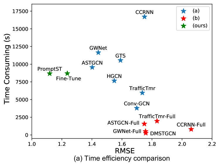
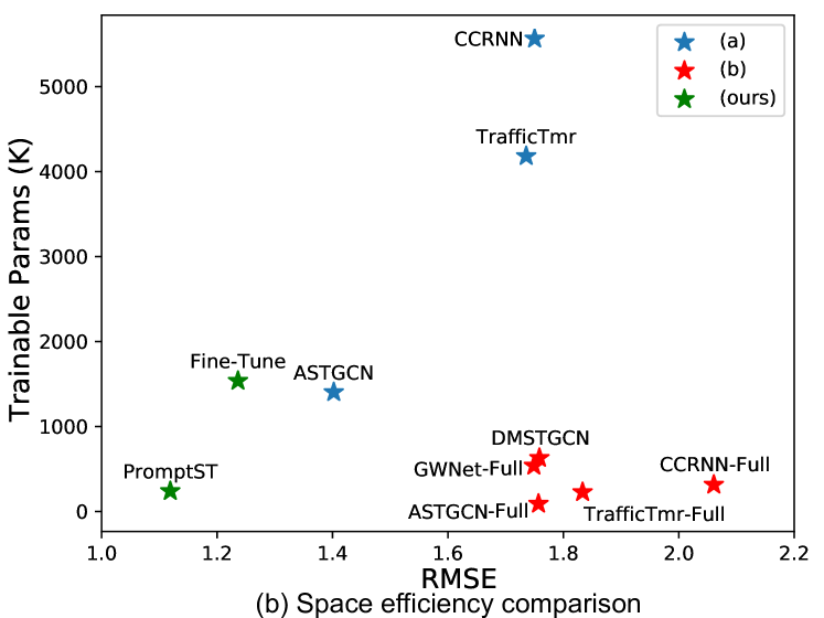
To evaluate our PromptST in the physical view, we compare the training time and total trainable parameters with the baselines, as shown in Figure 4. We present the performance on Complaint, which means for baselines in (a): training time and parameters are accumulations of individual training on 19 attributes; (b): results are from a single train on multi-attribute data; (ours) results consist of pretrain and individual tuning on 19 attributes. We omit Conv-GCN, HGCN, GWNet, and GTS in Figure 4 (b) due to their tremendously large parameters volume, the concrete number of which can be referred to Table 1. According to the efficiency comparison, (1) The advancing spatio-temporal prediction methods (blue stars) cost apparently more than their multi-attribute versions (red stars), while achieving consistently better results. (2) As promising spatio-temporal multi-attribute solutions, fine-tuned spatio-temporal transformer and our PromptST take the relatively leading position. (3) Our PromptST achieves the best performance with trivial trainable parameters and comparable training hours.
4.8. Hyper-Parameter Analysis
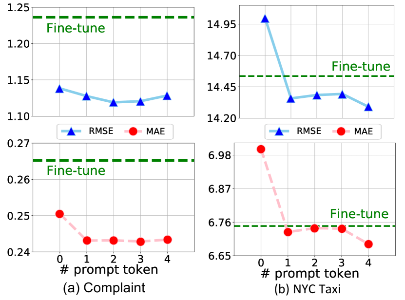
To further verify the efficacy of PromptST, we illustrate how the number of prompt tokens influences the performance of PromptST in this subsection. Figure 5 indicates the performance of PromptST with different numbers of spatio-temporal prompt tokens on the two datasets. We present the average RMSE and MAE of all the 19 attributes of Complaint, and the average value of 4 attributes of NYC Taxi. We test PromptST with in , where represents no prompt tokens inserted and only tuning head . For a clear understanding, we anchor the result of fine-tune as the red dashed line. Firstly, prompt tuning with all settings exceeds fine-tune, which proves the steady performance of PromptST. Furthermore, different numbers of lead to similar results, and we can observe a tiny turn as rises. Take Complaint for an example, PromptST achieves the best results at , and decreases as rises. The prompt tuning may overfit the target attribute to some extent as the number of prompt tokens rises.
5. Related Works
Spatio-Temporal Prediction. Spatio-temporal prediction plays a critical role in current city management, such as traffic prediction (Yu et al., 2017; Chai et al., 2018; Wang et al., 2021), weather prediction (Han et al., 2021b; Zheng et al., 2015; Liang et al., 2022), and next-POI recommendation (Zhang et al., 2021; Zhao et al., 2016b). Thanks to the apace boosting of deep learning techniques, recurrent neural networks (Ma et al., 2015; Tian and Pan, 2015) and 1-D convolutional network (Guo et al., 2019b; Yu et al., 2017) have been widely used in temporal information capture. Convolutional network (Zhang et al., 2017) and graph neural network (Guo et al., 2021a, 2019a) are generally incorporated to learn the spatial relationship.
Spatio-Temporal Multi-Task Learning. Recently, attention has been paid to spatio-temporal multi-task learning (Zhang et al., 2019; Wang et al., 2019; Zhang et al., 2020b). As one of the earliest efforts, GEML (Wang et al., 2019) devises LSTM to predict traffic on-demand flow. MDL (Zhang et al., 2020b) employs a convolutional neural network to predict both traffic flow and traffic on-demand flow simultaneously. Zhang et al. (Zhang et al., 2019) proposes to model the traffic pick-up and drop-off flows respectively with LSTM-based architecture and incorporates an MLP fusion layer for prediction. What’s more, there emerge multi-task learning methods for other spatio-temporal tasks. MasterGNN (Han et al., 2021b) utilizes a heterogeneous recurrent GNN to capture the spatio-temporal correlation between air quality and weather monitor stations. MATURE (Li et al., 2020) and KA2M2 (Li et al., 2021) propose to predict transportation mode with multi-task methods.
6. Conclusion
Spatio-temporal prediction plays a vital role in city management, but the analysis of diverse spatio-temporal attributes requires extensive expert efforts and economic costs. To alleviate this pain spot and explore the solution towards unified smart city modeling, we propose an efficient method, PromptST to solve spatio-temporal multi-attribute prediction. PromptST achieves a good balance between fitting the concrete attribute and maintaining the common knowledge. It also enjoys good transferability, which provides the potential to be extended to new spatio-temporal tasks.
Acknowledgements.
This research was partially supported by APRC - CityU New Research Initiatives (No.9610565, Start-up Grant for New Faculty of City University of Hong Kong), CityU - HKIDS Early Career Research Grant (No.9360163), Hong Kong ITC Innovation and Technology Fund Midstream Research Programme for Universities Project (No.ITS/034/22MS), SIRG - CityU Strategic Interdisciplinary Research Grant (No.7020046, No.7020074), SRG-Fd - CityU Strategic Research Grant (No.7005894), Tencent (CCF-Tencent Open Fund, Tencent Rhino-Bird Focused Research Fund), Huawei (Huawei Innovation Research Program), Ant Group (CCF-Ant Research Fund, Ant Group Research Fund) and Kuaishou. Hongwei Zhao is funded by the Provincial Science and Technology Innovation Special Fund Project of Jilin Province, grant number 20190302026GX, Natural Science Foundation of Jilin Province, grant number 20200201037JC, and the Fundamental Research Funds for the Central Universities, JLU. Zitao Liu is supported by National Key R&D Program of China, under Grant No. 2022YFC3303600, and Key Laboratory of Smart Education of Guangdong Higher Education Institutes, Jinan University (2022LSYS003).References
- (1)
- Aghajanyan et al. (2021) Armen Aghajanyan, Anchit Gupta, Akshat Shrivastava, Xilun Chen, Luke Zettlemoyer, and Sonal Gupta. 2021. Muppet: Massive Multi-task Representations with Pre-Finetuning. In Proceedings of the 2021 Conference on Empirical Methods in Natural Language Processing. Association for Computational Linguistics, 5799–5811. https://doi.org/10.18653/v1/2021.emnlp-main.468
- Ba et al. (2016) Jimmy Lei Ba, Jamie Ryan Kiros, and Geoffrey E Hinton. 2016. Layer normalization. arXiv preprint arXiv:1607.06450 (2016).
- Brown et al. (2020a) Tom Brown, Benjamin Mann, Nick Ryder, Melanie Subbiah, Jared D Kaplan, Prafulla Dhariwal, Arvind Neelakantan, Pranav Shyam, Girish Sastry, Amanda Askell, et al. 2020a. Language models are few-shot learners. Advances in neural information processing systems 33 (2020), 1877–1901.
- Brown et al. (2020b) Tom Brown, Benjamin Mann, Nick Ryder, Melanie Subbiah, Jared D Kaplan, Prafulla Dhariwal, Arvind Neelakantan, Pranav Shyam, Girish Sastry, Amanda Askell, et al. 2020b. Language models are few-shot learners. Advances in neural information processing systems 33 (2020), 1877–1901.
- Chai et al. (2018) Di Chai, Leye Wang, and Qiang Yang. 2018. Bike flow prediction with multi-graph convolutional networks. In Proceedings of the 26th ACM SIGSPATIAL international conference on advances in geographic information systems. 397–400.
- Chen et al. (2022) Changlu Chen, Yanbin Liu, Ling Chen, and Chengqi Zhang. 2022. Bidirectional spatial-temporal adaptive transformer for Urban traffic flow forecasting. IEEE Transactions on Neural Networks and Learning Systems (2022).
- Gao et al. (2021) Tianyu Gao, Adam Fisch, and Danqi Chen. 2021. Making Pre-trained Language Models Better Few-shot Learners. In Proceedings of the 59th Annual Meeting of the Association for Computational Linguistics and the 11th International Joint Conference on Natural Language Processing (Volume 1: Long Papers). Association for Computational Linguistics, Online, 3816–3830. https://doi.org/10.18653/v1/2021.acl-long.295
- Guo et al. (2021a) Kan Guo, Yongli Hu, Yanfeng Sun, Sean Qian, Junbin Gao, and Baocai Yin. 2021a. Hierarchical graph convolution network for traffic forecasting. In Proceedings of the AAAI conference on artificial intelligence, Vol. 35. 151–159.
- Guo et al. (2019a) Shengnan Guo, Youfang Lin, Ning Feng, Chao Song, and Huaiyu Wan. 2019a. Attention based spatial-temporal graph convolutional networks for traffic flow forecasting. In Proceedings of the AAAI conference on artificial intelligence, Vol. 33. 922–929.
- Guo et al. (2019b) Shengnan Guo, Youfang Lin, Ning Feng, Chao Song, and Huaiyu Wan. 2019b. Attention based spatial-temporal graph convolutional networks for traffic flow forecasting. In Proceedings of the AAAI conference on artificial intelligence, Vol. 33. 922–929.
- Guo et al. (2021b) Shengnan Guo, Youfang Lin, Huaiyu Wan, Xiucheng Li, and Gao Cong. 2021b. Learning dynamics and heterogeneity of spatial-temporal graph data for traffic forecasting. IEEE Transactions on Knowledge and Data Engineering 34, 11 (2021), 5415–5428.
- Han et al. (2021b) Jindong Han, Hao Liu, Hengshu Zhu, Hui Xiong, and Dejing Dou. 2021b. Joint Air Quality and Weather Prediction Based on Multi-Adversarial Spatiotemporal Networks. In Proceedings of the 35th AAAI Conference on Artificial Intelligence.
- Han et al. (2021a) Liangzhe Han, Bowen Du, Leilei Sun, Yanjie Fu, Yisheng Lv, and Hui Xiong. 2021a. Dynamic and multi-faceted spatio-temporal deep learning for traffic speed forecasting. In Proceedings of the 27th ACM SIGKDD conference on knowledge discovery & data mining. 547–555.
- Han et al. (2023) Xiao Han, Xiangyu Zhao, Liang Zhang, and Wanyu Wang. 2023. Mitigating Action Hysteresis in Traffic Signal Control with Traffic Predictive Reinforcement Learning. 673–684.
- He et al. (2016) Kaiming He, Xiangyu Zhang, Shaoqing Ren, and Jian Sun. 2016. Deep residual learning for image recognition. In Proceedings of the IEEE conference on computer vision and pattern recognition. 770–778.
- Jia et al. (2022) Menglin Jia, Luming Tang, Bor-Chun Chen, Claire Cardie, Serge Belongie, Bharath Hariharan, and Ser-Nam Lim. 2022. Visual Prompt Tuning. In Computer Vision – ECCV 2022: 17th European Conference, Tel Aviv, Israel, October 23–27, 2022, Proceedings, Part XXXIII (Tel Aviv, Israel). Springer-Verlag, Berlin, Heidelberg, 709–727. https://doi.org/10.1007/978-3-031-19827-4_41
- Lan et al. (2022) Shiyong Lan, Yitong Ma, Weikang Huang, Wenwu Wang, Hongyu Yang, and Pyang Li. 2022. Dstagnn: Dynamic spatial-temporal aware graph neural network for traffic flow forecasting. In International Conference on Machine Learning. PMLR, 11906–11917.
- Li et al. (2020) Can Li, Lei Bai, Wei Liu, Lina Yao, and S Travis Waller. 2020. Knowledge adaption for demand prediction based on multi-task memory neural network. In Proceedings of the 29th ACM international conference on information & knowledge management. 715–724.
- Li et al. (2021) Can Li, Lei Bai, Wei Liu, Lina Yao, and S Travis Waller. 2021. A multi-task memory network with knowledge adaptation for multimodal demand forecasting. Transportation Research Part C: Emerging Technologies 131 (2021), 103352.
- Li and Liang (2021) Xiang Lisa Li and Percy Liang. 2021. Prefix-Tuning: Optimizing Continuous Prompts for Generation. Proceedings of the 59th Annual Meeting of the Association for Computational Linguistics and the 11th International Joint Conference on Natural Language Processing (Volume 1: Long Papers) abs/2101.00190 (2021).
- Liang et al. (2022) Yuxuan Liang, Yutong Xia, Songyu Ke, Yiwei Wang, Qingsong Wen, Junbo Zhang, Yu Zheng, and Roger Zimmermann. 2022. AirFormer: Predicting Nationwide Air Quality in China with Transformers. arXiv preprint arXiv:2211.15979 (2022).
- Liu and Li (2020) Hui Liu and Yanfei Li. 2020. Smart cities for emergency management. Nature 578, 7796 (2020), 515–516.
- Liu et al. (2023) Pengfei Liu, Weizhe Yuan, Jinlan Fu, Zhengbao Jiang, Hiroaki Hayashi, and Graham Neubig. 2023. Pre-train, prompt, and predict: A systematic survey of prompting methods in natural language processing. Comput. Surveys 55, 9 (2023), 1–35.
- Ma et al. (2015) Xiaolei Ma, Zhimin Tao, Yinhai Wang, Haiyang Yu, and Yunpeng Wang. 2015. Long short-term memory neural network for traffic speed prediction using remote microwave sensor data. Transportation Research Part C: Emerging Technologies 54 (2015), 187–197.
- McCloskey and Cohen (1989) Michael McCloskey and Neal J Cohen. 1989. Catastrophic interference in connectionist networks: The sequential learning problem. In Psychology of learning and motivation. Vol. 24. Elsevier, 109–165.
- Petroni et al. (2019) Fabio Petroni, Tim Rocktäschel, Sebastian Riedel, Patrick S. H. Lewis, Anton Bakhtin, Yuxiang Wu, and Alexander H. Miller. 2019. Language Models as Knowledge Bases?. In Proceedings of the 2019 Conference on Empirical Methods in Natural Language Processing and the 9th International Joint Conference on Natural Language Processing, EMNLP-IJCNLP 2019, Hong Kong, China, November 3-7, 2019. Association for Computational Linguistics, 2463–2473. https://doi.org/10.18653/v1/D19-1250
- Ramasesh et al. (2021) Vinay Venkatesh Ramasesh, Aitor Lewkowycz, and Ethan Dyer. 2021. Effect of scale on catastrophic forgetting in neural networks. In International Conference on Learning Representations.
- Shang and Chen (2021) Chao Shang and Jie Chen. 2021. Discrete Graph Structure Learning for Forecasting Multiple Time Series. In Proceedings of International Conference on Learning Representations.
- Shao et al. (2022) Zezhi Shao, Zhao Zhang, Fei Wang, and Yongjun Xu. 2022. Pre-training enhanced spatial-temporal graph neural network for multivariate time series forecasting. In Proceedings of the 28th ACM SIGKDD Conference on Knowledge Discovery and Data Mining. 1567–1577.
- Shen et al. (2021) Zhiqiang Shen, Zechun Liu, Jie Qin, Marios Savvides, and Kwang-Ting Cheng. 2021. Partial Is Better Than All: Revisiting Fine-tuning Strategy for Few-shot Learning. Proceedings of the AAAI Conference on Artificial Intelligence 35, 11 (May 2021), 9594–9602. https://doi.org/10.1609/aaai.v35i11.17155
- Sun et al. (2019) Chi Sun, Xipeng Qiu, Yige Xu, and Xuanjing Huang. 2019. How to fine-tune bert for text classification?. In China national conference on Chinese computational linguistics. Springer, 194–206.
- Tascikaraoglu (2018) Akin Tascikaraoglu. 2018. Evaluation of spatio-temporal forecasting methods in various smart city applications. Renewable and Sustainable Energy Reviews 82 (2018), 424–435.
- Tian and Pan (2015) Yongxue Tian and Li Pan. 2015. Predicting short-term traffic flow by long short-term memory recurrent neural network. In 2015 IEEE international conference on smart city/SocialCom/SustainCom (SmartCity). IEEE, 153–158.
- Vaswani et al. (2017) Ashish Vaswani, Noam Shazeer, Niki Parmar, Jakob Uszkoreit, Llion Jones, Aidan N Gomez, Łukasz Kaiser, and Illia Polosukhin. 2017. Attention is all you need. Advances in neural information processing systems 30 (2017).
- Wang et al. (2022) Peng Wang, An Yang, Rui Men, Junyang Lin, Shuai Bai, Zhikang Li, Jianxin Ma, Chang Zhou, Jingren Zhou, and Hongxia Yang. 2022. Ofa: Unifying architectures, tasks, and modalities through a simple sequence-to-sequence learning framework. In International Conference on Machine Learning. PMLR, 23318–23340.
- Wang et al. (2020) Senzhang Wang, Hao Miao, Hao Chen, and Zhiqiu Huang. 2020. Multi-task adversarial spatial-temporal networks for crowd flow prediction. In Proceedings of the 29th ACM international conference on information & knowledge management. 1555–1564.
- Wang et al. (2021) Senzhang Wang, Jiaqiang Zhang, Jiyue Li, Hao Miao, and Jiannong Cao. 2021. Traffic Accident Risk Prediction via Multi-View Multi-Task Spatio-Temporal Networks. IEEE Transactions on Knowledge and Data Engineering (2021).
- Wang et al. (2019) Yuandong Wang, Hongzhi Yin, Hongxu Chen, Tianyu Wo, Jie Xu, and Kai Zheng. 2019. Origin-destination matrix prediction via graph convolution: a new perspective of passenger demand modeling. In Proceedings of the 25th ACM SIGKDD international conference on knowledge discovery & data mining. 1227–1235.
- Wu et al. (2019) Zonghan Wu, Shirui Pan, Guodong Long, Jing Jiang, and Chengqi Zhang. 2019. Graph WaveNet for Deep Spatial-Temporal Graph Modeling. In Proceedings of the Twenty-Eighth International Joint Conference on Artificial Intelligence, IJCAI-19. International Joint Conferences on Artificial Intelligence Organization, 1907–1913. https://doi.org/10.24963/ijcai.2019/264
- Yan et al. (2022) Bin Yan, Yi Jiang, Peize Sun, Dong Wang, Zehuan Yuan, Ping Luo, and Huchuan Lu. 2022. Towards grand unification of object tracking. In Computer Vision–ECCV 2022: 17th European Conference, Tel Aviv, Israel, October 23–27, 2022, Proceedings, Part XXI. Springer, 733–751.
- Yan et al. (2021) Haoyang Yan, Xiaolei Ma, and Ziyuan Pu. 2021. Learning dynamic and hierarchical traffic spatiotemporal features with transformer. IEEE Transactions on Intelligent Transportation Systems (2021).
- Ye et al. (2021) Junchen Ye, Leilei Sun, Bowen Du, Yanjie Fu, and Hui Xiong. 2021. Coupled layer-wise graph convolution for transportation demand prediction. In Proceedings of the AAAI conference on artificial intelligence, Vol. 35. 4617–4625.
- Yu et al. (2017) Bing Yu, Haoteng Yin, and Zhanxing Zhu. 2017. Spatio-temporal graph convolutional networks: A deep learning framework for traffic forecasting. arXiv preprint arXiv:1709.04875 (2017).
- Zhang et al. (2020b) Chizhan Zhang, Fenghua Zhu, Xiao Wang, Leilei Sun, Haina Tang, and Yisheng Lv. 2020b. Taxi demand prediction using parallel multi-task learning model. IEEE Transactions on Intelligent Transportation Systems (2020).
- Zhang et al. (2020a) Jinlei Zhang, Feng Chen, Yinan Guo, and Xiaohong Li. 2020a. Multi-graph convolutional network for short-term passenger flow forecasting in urban rail transit. IET Intelligent Transport Systems 14, 10 (2020), 1210–1217.
- Zhang et al. (2017) Junbo Zhang, Yu Zheng, and Dekang Qi. 2017. Deep spatio-temporal residual networks for citywide crowd flows prediction. In Thirty-first AAAI conference on artificial intelligence.
- Zhang et al. (2019) Junbo Zhang, Yu Zheng, Junkai Sun, and Dekang Qi. 2019. Flow prediction in spatio-temporal networks based on multitask deep learning. IEEE Transactions on Knowledge and Data Engineering 32, 3 (2019), 468–478.
- Zhang et al. (2021) Lu Zhang, Zhu Sun, Jie Zhang, Yu Lei, Chen Li, Ziqing Wu, Horst Kloeden, and Felix Klanner. 2021. An interactive multi-task learning framework for next POI recommendation with uncertain check-ins. In Proceedings of the Twenty-Ninth International Conference on International Joint Conferences on Artificial Intelligence. 3551–3557.
- Zhang et al. (2023) Zijian Zhang, Xiangyu Zhao, Hao Miao, Chunxu Zhang, Hongwei Zhao, and Junbo Zhang. 2023. AutoSTL: Automated Spatio-Temporal Multi-Task Learning. Proceedings of the AAAI Conference on Artificial Intelligence 37, 4 (Jun. 2023), 4902–4910. https://doi.org/10.1609/aaai.v37i4.25616
- Zhao et al. (2016b) Shenglin Zhao, Tong Zhao, Haiqin Yang, Michael R Lyu, and Irwin King. 2016b. STELLAR: Spatial-temporal latent ranking for successive point-of-interest recommendation. In Thirtieth AAAI conference on artificial intelligence.
- Zhao et al. (2022) Xiangyu Zhao, Wenqi Fan, Hui Liu, and Jiliang Tang. 2022. Multi-type Urban Crime Prediction. In Proceedings of the AAAI Conference on Artificial Intelligence, Vol. 36. 4388–4396.
- Zhao and Tang (2017a) Xiangyu Zhao and Jiliang Tang. 2017a. Exploring Transfer Learning for Crime Prediction. In 2017 IEEE International Conference on Data Mining Workshops (ICDMW). IEEE, 1158–1159.
- Zhao and Tang (2017b) Xiangyu Zhao and Jiliang Tang. 2017b. Modeling Temporal-Spatial Correlations for Crime Prediction. In Proceedings of the 2017 ACM on Conference on Information and Knowledge Management. ACM, 497–506.
- Zhao and Tang (2018) Xiangyu Zhao and Jiliang Tang. 2018. Crime in Urban Areas:: A Data Mining Perspective. ACM SIGKDD Explorations Newsletter 20, 1 (2018), 1–12.
- Zhao et al. (2017) Xiangyu Zhao, Tong Xu, Yanjie Fu, Enhong Chen, and Hao Guo. 2017. Incorporating Spatio-Temporal Smoothness for Air Quality Inference. In 2017 IEEE International Conference on Data Mining (ICDM). IEEE, 1177–1182.
- Zhao et al. (2016a) Xiangyu Zhao, Tong Xu, Qi Liu, and Hao Guo. 2016a. Exploring the Choice Under Conflict for Social Event Participation. In International Conference on Database Systems for Advanced Applications. Springer, 396–411.
- Zheng et al. (2020) Chuanpan Zheng, Xiaoliang Fan, Cheng Wang, and Jianzhong Qi. 2020. Gman: A graph multi-attention network for traffic prediction. In Proceedings of the AAAI conference on artificial intelligence, Vol. 34. 1234–1241.
- Zheng et al. (2015) Yu Zheng, Xiuwen Yi, Ming Li, Ruiyuan Li, Zhangqing Shan, Eric Chang, and Tianrui Li. 2015. Forecasting fine-grained air quality based on big data. In Proceedings of the 21th ACM SIGKDD international conference on knowledge discovery and data mining. 2267–2276.
- Zhou et al. (2021) Haoyi Zhou, Shanghang Zhang, Jieqi Peng, Shuai Zhang, Jianxin Li, Hui Xiong, and Wancai Zhang. 2021. Informer: Beyond efficient transformer for long sequence time-series forecasting. In Proceedings of the AAAI Conference on Artificial Intelligence, Vol. 35. 11106–11115.