On a Continuum Model for Random Genetic Drift: A Dynamical Boundary Condition Approach

Abstract

We propose a new continuum model for a random genetic drift problem by employing a dynamical boundary condition approach. The new model can be viewed as a regularized Kimura equation, which admits a continuous solution and recovers the original system in the limits. The existence and uniqueness of the strong solution of the regularized system are shown. Finally, we present some numerical results for the regularized model, which indicates that the model can capture the main features of the original model, include gene fixation and conservation of the first moment.

1 Introduction

Genetic drift is a fundamental process in molecular evolution [11]. It refers to the random fluctuations in allele frequencies within a population over time. Typical mathematical models for genetic drift include the Wright–Fisher model [13, 26] and its diffusion limit, known as the Kimura equation [27, 15].

Without mutation, migration, and selection process, the Kimura equation can be written as [11]

(1) $$\partial_{t}\rho=\partial_{xx}^{2}(x(1-x)\rho)\ ,\quad x\in(0,1)\ ,\ t>0\ .$$

Here, the variable $x$ is the fraction of the focal allele $A_{1}$ in the population and $(1-x)$ is that of $A_{2}$, the function $\rho(x,t)$ is the probability of finding a relative composition $x\in[0,1]$ of gene $A_{1}$ at time $t$. Although (1) is a linear PDE of $\rho(x,t)$, due to the degeneracy of $x(1-x)$ at the boundary $x=0$ and $x=1$ [7, 8], it is difficult to impose a suitable boundary condition [12]. In[17], Kolmogorov suggested that the equation (10) is only reasonable for $x$ not too close to $0$ and $1$.

To maintain the biological significance, $\rho(x,t)$ satisfies the mass conservation

(2) $$\int_{0}^{1}\rho(x,t)\mathrm{d}x=1\ ,$$

which suggests a possible non-flux boundary to (1), given by

(3) $$\partial_{x}(x(1-x)\rho)=0\ ,\quad x=0~{}\text{or}~{}1\ ,\quad\forall t\ .$$

However, such a boundary condition excludes the existence of regular solution of (1). In [18, 4], the authors prove that for a given $\rho_{0}\in\mathcal{BM}^{+}([0,1])$, there exists a unique solution to (1) with $\rho(x,t)\in L^{\infty}([0,\infty),\mathcal{BM}^{+}([0,1]))$, and the solution $\rho(x,t)$ can be expressed as

(4) $$\rho(x,t)=q(x,t)+a(t)\delta_{0}+b(t)\delta_{1}\ .$$

Here $\mathcal{BM}^{+}([0,1])$ is the space of all (positive) Radon measures on $[0,1]$, $\delta_{0}$ and $\delta_{1}$ are Dirac delta function at 0 and 1 respectively, and $q(x,t)\in C^{\infty}(\mathbb{R}^{+};C^{\infty}([0,1]))$ is a classical solution to (1). Moreover, it is proved that [4], as $t\rightarrow\infty$, $q(x,t)\rightarrow 0$ uniformly, and $a(t)$ and $b(t)$ are monotonically increasing function such that

(5) $$a^{\infty}=\lim_{t\rightarrow\infty}a(t)=\int_{0}^{1}(1-x)\rho_{0}(x)\mathrm{d}x\ ,$$

$$b^{\infty}=\lim_{t\rightarrow\infty}b(t)=\int_{0}^{1}x\rho_{0}(x)\mathrm{d}x\ .$$

The equilibrium (5) is determined by the fact that the Kimura equation (1) preserves the first moment of the probability density [4]. Indeed, a direct computation shows that

(6) $$\frac{\mathrm{d}}{\mathrm{d}t}\int_{0}^{1}x\rho(x,t)\mathrm{d}x=\int_{0}^{1}x\partial_{xx}^{2}(x(1-x)\rho)\mathrm{d}x$$

$$=\int_{0}^{1}\partial_{xx}(x)(x(1-x)\rho)\mathrm{d}x-\partial_{x}(x)\partial_{x}(x(1-x)\rho)\Big{|}_{0}^{1}+x(\partial_{x}(x(1-x)\rho))\Big{|}_{0}^{1}=0.$$

In biology, the function $\psi(x)=x$ is known as the fixation probability function, which describes the probability of allele $A_{1}$ fixing in a population while allele $A_{2}$ goes extinct, under the condition of starting from an initial composition of $x$.

The measure-valued solution (4) imposed a difficulty to study Kimura equation both numerically [6] and theoretically [2]. For instance, although a lot of different methods for the Kimura equation have been developed, ranging from finite volume method [28, 29], finite Lagrangian methods [6], an optimal mass transportation method [1], and SDE–based simulation methods [5, 14], it is difficult to get a good numerical approximation to (4), which includes Dirac delta function, and accurately capture the dynamics of $a(t)$ and $b(t)$.

The purpose of this paper is to propose a new continuum model for random genetic drift by incorporating a dynamical boundary to Kimura equation. The new model is given by

(7) $$\begin{cases}&\rho_{t}=\partial_{xx}^{2}(x(1-x)\rho),\quad x\in(\delta,1-\delta),\\ &\rho u(\delta,t)=-a^{\prime}(t),\quad\rho u(1-\delta,t)=b^{\prime}(t)\\ &a^{\prime}(t)=-((\epsilon a)-\rho(\delta,t))\\ &b^{\prime}(t)=-((\epsilon b)-\rho(1-\delta,t)).\\ \end{cases}$$

Here $\delta$ and $\epsilon$ are artificial small parameters. The key idea is to introduce an additional jump process between bulk and surface, which leads to dynamical boundary condition. Such a regularized Kimura equation admits a classical solution for fixed $\epsilon$ and $\delta$, and can be solved by a standard numerical scheme. Formally, the original Kimura equation can be viewed as a singular limit of $\epsilon\rightarrow 0$ and $\delta\rightarrow 0$. Numerical tests show that the qualitative behaviors of the original Kimura equation, such as gene fixation and conservation of first moment, can be well captured with small $\epsilon$ and $\delta$.

The rest of this paper is organized as follows. In Section 2, we introduce a few background, including the Wright-Fisher model, the variational structure of Kimura equation, and the dynamical boundary approach for generalized diffusions. The new continuum model is presented in Section 3. The existence and uniqueness of the strong solution of the regularized system is shown in section 4. Finally, we perform a numerical study to the regularized system, and demonstrated the effects of $\delta$ and $\epsilon$, as well as the ability of new model in capturing the key feature of the original Kimura equation.

2 Background

2.1 From a Wright-Fisher model to Kimura equation

We first briefly review the formal derivation of Kimura equation from the Wright-Fisher model. Consider two competing alleles, denoted by $A_{1}$ and $A_{2}$, in a diploid population with fixed size $N$ (i.e., total $2N$ alleles). Assume $u$ and $v$ are the probability of mutations $A_{1}\rightarrow A_{2}$ and $A_{2}\rightarrow A_{1}$ respectively. Let $X_{k}$ be the portion of individuals of type $A_{1}$ in generation $k$. The original Wright-Fisher model describes random fluctuations in the genetic expression by a discrete-time, discrete-state Markov chain. The discrete state space is defined as $I=\{0,\frac{1}{2N},\ldots,1\}$, and the transition probability is given by [12, 9]

(8) $$\mathbb{P}\left(X_{k+1}=\frac{j}{2N}~{}\Big{|}X_{k}=\frac{i}{2N}\right)=\tbinom{2N}{j}p_{i}^{j}(1-p_{i})^{2N-j}\ ,$$

where

(9) $$p_{i}=(1-u)\frac{i}{2N}+v(1-\frac{i}{2N})\ .$$

In the case that $u=v=0$ (without mutations), we have

(10) $$\mathbb{P}\left(X_{k+1}=\frac{j}{M}~{}\Big{|}X_{k}=\frac{i}{2N}\right)=\tbinom{2N}{j}(\frac{i}{2N})^{j}(1-\frac{i}{2N})^{2N-j}\ ,$$

This is known as the pure drift case. Notice that in the pure drift case, the jump rate becomes 0 if $X_{k}=0$ or $X_{k}=1$, which are absorbing states in the system. There is no possibility of fixations if $u>0$ and $v>0$.

When the population size $N$ is large, the Wright-Fisher model can be approximated by a continuous–state, continuous–time process $X(t)$, which represents the proportion of alleles of type $A_{1}$, at least formally. The dynamics of $X(t)$ is described by an SDE [5]

(11) $$\mathrm{d}X_{t}=(u-(u+v)X_{t})\mathrm{d}t+\sqrt{X_{t}(1-X_{t})}\mathrm{d}W_{t}$$

The corresponding Fokker-Planck equation is given by [9, 21]

(12) $$\rho_{t}+\partial_{x}((u(1-x)-vx)\rho)=\frac{1}{2}\partial_{x}(x(1-x)\rho).$$

For the pure diffusion case, we obtain a Kimura equation

(13) $$\partial_{t}\rho=\frac{1}{2}\partial_{xx}^{2}(x(1-x)\rho),\quad x\in(0,1),t>0,$$

It is convenient to re-scale the time by letting $t^{\prime}=2t$, and the Kimura equation (10) becomes (1).

2.2 Formal Variational Structure

Formally, the Kimura equation (1) can be viewed as a generalized diffusion, derive from the energy-dissipation law [6]

(14) $$\frac{\mathrm{d}}{\mathrm{d}t}\int_{0}^{1}\rho\ln\left(x(1-x)\rho\right)\mathrm{d}x=-\int_{0}^{1}\frac{\rho}{x(1-x)}|u|^{2}\mathrm{d}x\ ,$$

where the distribution $\rho$ satisfies the kinematics

(15) $$\partial_{t}\rho+\partial_{x}(\rho u)=0\ ,\quad x\in(0,1)$$

$$\rho u=0,\quad x=0~{}\text{or}~{}1\ .$$

Here the non-flux boundary $\rho u=0$ guarantees the mass conservation.

To obtain the Kimura equation from the energy-dissipation law (14), one needs to introduce a flow map denoted as $x(X,t):[0,1]\rightarrow[0,1]$ associated with the velocity field $u(x,t)$. For given $X$, the flow map satisfies the following ordinary differential equation:

(16) $$\frac{\mathrm{d}}{\mathrm{d}t}x(X,t)=u(x(X,t),t),\quad x(X,0)=X,$$

where $X$ represents the Lagrangian coordinate, and $x$ represents the Eulerian coordinate. Due to the mass conservation, $\rho(x(X,t),t)$ satisfies the kinematics

(17) $$\rho(x(X,t),t)=\rho_{0}(X)/\det F(X,t)\ ,\quad\det F(X,t)=\partial_{X}x(X,t)\ ,\quad X\in(0,1)$$

in Lagrangian coordinates, where $\rho_{0}(X)$ is the initial density. Recall $u(\bm{x}(X,t),t)=x_{t}(X,t)$, the energy-dissipation law can be written as

(18) $$\frac{\mathrm{d}}{\mathrm{d}t}\int\rho_{0}\ln(x(1-x))+\rho_{0}\ln(\rho_{0}/\partial_{X}x)\mathrm{d}X=-\int_{0}^{1}\frac{\rho_{0}}{x(1-x)}|x_{t}|^{2}\mathrm{d}x$$

in Lagrangian coordinates, which can be interpreted as an $L^{2}$-gradient flow in terms of $x(X,t)$. By a standard energetic variation procedure (see [6] for details), we can derive the force balance equation

(19) $$\frac{\rho}{x(1-x)}u=-\rho\partial_{x}(\ln(\rho x(1-x)))\ ,$$

which can be simplified as

(20) $$\rho u=-\partial_{x}(x(1-x)p)\ .$$

Combining the velocity equation with the kinematics (15), we can recover the original Kimura equation. The variational structure (18) naturally leads to the Lagrangian algorithms developed in [6, 1].

Alternatively, (14) can be interpreted a Wasserstein type of gradient flow, with the transport distance defined by

(21) $$d^{2}(\rho_{1},\rho_{2})=\mathop{\min}_{(\rho,\mathbf{u})}\int_{0}^{1}\int_{0}^{1}\frac{\rho}{x(1-x)}|u|^{2}\mathrm{d}x\mathrm{d}t~{},$$

$$\text{subject to}~{}\rho_{t}+\partial_{x}(\rho u)=0~{},\quad\rho(x,0)=\rho_{1}~{},\quad\rho(x,1)=\rho_{2}.$$

The distance (21) is known as Wasserstein-Shahshahani distance [3, 2].

As pointed out in [2], the variational structure presented in this subsection is rather formal. Although we can define $U(x)=\ln(x(1-x))$ [2, 22], which plays the role of internal energy as in standard Fokker-Planck equation, the system doesn’t admit a unique equilibrium distribution $\rho^{\rm eq}\approx\exp(-U)$, as $\int_{0}^{1}\frac{1}{x(1-x)}\mathrm{d}x$ is unbounded.

2.3 Dynamical boundary condition

As suggested in [2], a natural attempt at compensating for singularities is to relax the boundary condition by taking account of the bulk/surface interaction into model.

Before we present the application of the dynamical boundary condition approach to the Kimura model, we first briefly review of the dynamical boundary approach for generalized diffusions in this subsection. Consider a bounded domain $\Omega$, and let $\Gamma=\partial\Omega$ be the boundary of $\Omega$. Classical PDE models on $\Omega$ often impose Dirichlet, Neumann, and Robin boundary conditions for physical variable $\rho$. The basic fundamental assumption behind this is $\rho$ is regular enough (e.g. $\rho\in C^{m}(\bar{\Omega})$ for some $m$), so we can define $\rho|_{\Gamma}$ as the trace of $\rho$, and we can define the boundary condition in terms of $\rho|_{\Gamma}$. However, as in the classical Kimura equation, it may not be always possible to take the trace.

The idea of dynamical boundary condition is to introduce another function $\sigma\in C(\Gamma)$ to describe the surface densities on the boundary, and view the exchange between bulk and surface density as a chemical reaction $\rho\ce{<=>}\sigma$ [16, 24]. Due to the mass conservation, $\rho$ and $\sigma$ satisfies

(22) $$\frac{\mathrm{d}}{\mathrm{d}t}\left(\int_{\Omega}\rho\mathrm{d}\bm{x}+\int_{\Gamma}\sigma\mathrm{d}S\right)=0,$$

which leads to the kinematics in Eulerian coordinates

(23) $$\rho_{t}+\nabla\cdot(\rho\mathbf{u})=0,~{}~{}\bm{x}\in\Omega,$$

$$\rho\mathbf{u}\cdot{\bm{\nu}}=R_{t},\quad\sigma_{t}+\nabla_{\Gamma}\cdot(\sigma{\bm{v}}_{\Gamma})=R_{t},~{}~{}\bm{x}\in\Gamma$$

where ${\bm{\nu}}$ is the outer normal of $\Omega$ and $R$ is the reaction trajectory for the chemical reaction $\rho\ce{<=>}\sigma$ that represents the density exchange between bulk and surface [25].

In general, systems with dynamical boundary condition can be modeled through an energy-dissipation law

(24) $$\frac{\mathrm{d}}{\mathrm{d}t}\left(\mathcal{F}_{b}(\rho)+\mathcal{F}_{s}(\sigma)\right)=-\left(\int_{\Omega}\eta_{b}(\rho)|\mathbf{u}|^{2}\mathrm{d}\bm{x}+\int_{\partial\Omega}\eta_{s}(\sigma)|{\bm{v}}|^{2}+R_{t}\Psi(R,R_{t})\mathrm{d}S\right)$$

Here $\mathcal{F}_{b}(\rho)$ and $\mathcal{F}_{s}(\sigma)$ are free energies in the bulk and surface respectively, $\eta_{b}(\rho)>0$ and $\eta_{s}(\sigma)>0$ are friction coefficients for bulk and surface diffusions, $R_{t}\Psi(R,R_{t})\geq 0$ is the dissipation due to the bulk/surface interaction, which in general is non-quadratic in terms of $R_{t}$ [25]. An energetic variational procedure leads to the force balance equations for the mechanical and chemical parts

(25) $$\begin{cases}&\eta_{b}(\rho)\mathbf{u}=-\rho\nabla\mu_{b}(\rho),\quad\mu_{b}=\frac{\delta\mathcal{F}_{b}}{\delta\rho}\quad\bm{x}\in\Omega\\ &\eta_{s}(\sigma){\bm{v}}=-\sigma\nabla_{\Gamma}\mu_{s}(\sigma),\quad\mu_{s}=\frac{\delta\mathcal{F}_{s}}{\delta\sigma},\quad\bm{x}\in\Gamma\\ &\Psi(R,R_{t})=-(\mu_{s}(\sigma)-\mu_{b}(\rho)),\quad\bm{x}\in\Gamma\\ \end{cases}$$

where $\mu_{s}(\sigma)-\mu_{b}(\rho)$ is the affinity of the bulk-surface reaction. Different choices of the free energy and the dissipation lead to different systems [24].

3 A regularized Kimura equation

In this section, we propose a regularized Kimura equation by applying a dynamical boundary condition approach in this specific one dimensional setting.

For a given $\delta>0$, let $\rho(x,t)$ represent the probability at $x$ for $x\in(\delta,1-\delta)$. We denote the probabilities at $x=0$ and $x=1$ as $a(t)$ and $b(t)$, respectively. Due to the conservation of mass, we have

(26) $$\frac{\mathrm{d}}{\mathrm{d}t}\left(\int_{\delta}^{1-\delta}\rho(x,t)\mathrm{d}x+a(t)+b(t)\right)=0$$

which is the consequence of the following kinematics conditions

(27) $$\partial_{t}\rho+\partial_{x}(\rho u)=0,\quad x\in(\delta,1-\delta)$$

$$\rho u(\delta,t)=-\dot{R}_{0},\quad\rho u(1-\delta,t)=\dot{R}_{1}(t)$$

$$a^{\prime}(t)=\dot{R}_{0},\quad b^{\prime}(t)=\dot{R}_{1}(t)$$

Here $R_{0}(t)$ and $R_{1}(t)$ denotes the reaction trajectory from $x=\delta$ to $x=0$ and from $x=1-\delta$ to $x=1$ respectively. It is worth mentioning that $\delta$ is a rather artificial regularization parameter.

The overall system can be modeled through the energy-dissipation law

(28) $$\frac{\mathrm{d}}{\mathrm{d}t}\int_{\delta}^{1-\delta}\rho\ln\left(x(1-x)\rho\right)\mathrm{d}x+G_{0}(a)+G_{1}(b)$$

$$=-\int_{\delta}^{1-\delta}\frac{\rho}{x(1-x)}|u|^{2}\mathrm{d}x-\Gamma_{0}(R_{0},\dot{R_{0}})-\Gamma_{1}(R_{1},\dot{R_{1}})$$

where $G_{0}(a)$ and $G_{1}(b)$ are free energy on the boundary, and $\Gamma_{0}(R_{0},\dot{R}_{0})$ and $\Gamma_{1}(R_{1},\dot{R}_{1})$ are dissipations on due to the bulk/surface jump. The energy-dissipation law in the bulk region ($x\in(\delta,1-\delta)$) is exactly same to the one in the original Kimura equation (14). The remaining question is how choose $G_{i}(i=0,1)$ and $\Gamma_{i}(i=0,1)$ to capture the qualitative behavior of the original Kimura equation. In the current work, we take

(29) $$G_{0}(q)=G_{1}(q)=G(q)=q\ln(\epsilon\delta(1-\delta)q)\ ,$$

and

(30) $$\Gamma_{0}(R,\dot{R})=\dot{R}\ln\left(\frac{\dot{R}_{t}}{\gamma_{0}a}+1\right),\quad\Gamma_{1}(R,\dot{R})=\dot{R}\ln\left(\frac{\dot{R}}{\gamma_{1}b}+1\right)\ .$$

Here $\gamma_{0}$ and $\gamma_{1}$ are reaction rate from surface to bulk. In the current study, we take $\gamma_{0}=\gamma_{1}=\epsilon$. We’ll study the effects of $\gamma_{0}$ and $\gamma_{1}$ in the future work.

By an energetic variational procedure [24], we can obtain the velocity equation

(31) $$\rho u=-\partial_{x}(x(1-x)\rho),\quad x\in(\delta,1-\delta),$$

and the equations for reaction rates

(32) $$\ln\left(\frac{\dot{R}_{0}}{\epsilon a}+1\right)=-(\ln(\epsilon a)-\ln\rho(\delta,t))$$

$$\ln\left(\frac{\dot{R}_{1}}{\epsilon b}+1\right)=-(\ln(\epsilon b)-\ln p(1-\delta,t))$$

One can rewrite (32) as

(33) $$\dot{R}_{0}=\rho(\delta,t)-\epsilon a,\quad\dot{R}_{1}=\rho(1-\delta,t)-\epsilon b\ .$$

Combing (31) and (33) with the kinematics (27), one arrives the final equation

(34) $$\begin{cases}&\partial_{t}\rho=-\partial_{x}(\rho u),\quad x\in[\delta,1-\delta]\\ &\rho u=-\partial_{x}(x(1-x)\rho),\quad x\in(\delta,1-\delta),\\ &\rho u(\delta,t)=-a^{\prime}(t),\quad\rho u(1-\delta,t)=b^{\prime}(t)\\ &a^{\prime}(t)=\rho(\delta,t)-\epsilon a\\ &b^{\prime}(t)=\rho(1-\delta,t)-\epsilon b\\ \end{cases}$$

Remark 3.1.

One import feature of the original Kimura equation that it also preserves the first moment, i.e., $\frac{\mathrm{d}}{\mathrm{d}t}\int x\rho\mathrm{d}x=0$. For the regularized system (34), a direct calculation shows that for $\psi(x)=x$,

(35) $$\frac{\mathrm{d}}{\mathrm{d}t}\int_{\delta}^{1-\delta}\psi(x)\rho(x,t)\mathrm{d}x+a\psi(0)+b\psi(1)$$

$$=\int_{\delta}^{1-\delta}-\partial_{x}\psi(x)\partial_{x}(x(1-x)p)\mathrm{d}x-\psi(x)(pu)\Big{|}_{\delta}^{1-\delta}+a^{\prime}(t)\psi(0)+b^{\prime}(t)\psi(1)$$

$$=\int_{\delta}^{1-\delta}\partial_{xx}\psi(x)(x(1-x)p)\mathrm{d}x-\partial_{x}\psi(x)(x(1-x)p)\Big{|}_{\delta}^{1-\delta}+\delta(b^{\prime}(t)-a^{\prime}(t))$$

$$=-\delta(1-\delta)(p(1-\delta)-p(\delta))+\delta(b^{\prime}(t)-a^{\prime}(t)).$$

The regularized system (34) no longer preserves the first moment for $\delta>0$. However, numerical simulations show that the change in first moment will be very small if $\delta$ is small.

For the regularized system (34), since

(36) $$a^{\prime}(t)+\epsilon a=\rho(\delta,t)$$

we have

(37) $$a(t)=e^{-\epsilon t}\int_{0}^{t}e^{\epsilon s}\rho(\delta,s)\mathrm{d}s$$

with the initial condition $a(0)=0$. As a consequence

(38) $$a^{\prime}(t)=-\epsilon e^{-\epsilon t}\int_{0}^{t}e^{\epsilon s}\rho(\delta,s)\mathrm{d}s+\rho(\delta,t)$$

Hence, the boundary condition can be interpreted as a delayed boundary condition

(39) $$pu(\delta,t)=\epsilon e^{-\epsilon t}\int_{0}^{t}e^{\epsilon s}\rho(\delta,s)\mathrm{d}s-\rho(\delta,t)$$

Remark 3.2.

If $\epsilon=0$, the equation becomes

(40) $$\begin{cases}&\partial_{t}\rho=-\partial_{x}(\rho u),\quad x\in(\delta,1-\delta)\\ &\rho u=-\partial_{x}(x(1-x)\rho),\quad x\in(\delta,1-\delta),\\ &\rho u(\delta,t)=-\rho(\delta,t),\quad\rho u(1-\delta,t)=\rho(1-\delta,t)\\ &a^{\prime}(t)=\rho(\delta,t)\\ &b^{\prime}(t)=\rho(1-\delta,t)\ .\\ \end{cases}$$

But the energy-dissipation law (28) with (29) is no longer valid in this limiting case.

Next, we perform some formal analysis to the regularized model. At the equilibrium, we have

(41) $$\rho^{\infty}(\delta)=\epsilon a^{\infty},\quad\rho^{\infty}(1-\delta)=\epsilon b^{\infty},$$

and $\rho^{\infty}$ satisfies

(42) $$\partial_{xx}^{2}(x(1-x)\rho^{\infty})=0,\quad x\in(\delta,1-\delta)\ .$$

It is straightforward to show that the classical solution to (42) is given by

(43) $$\rho^{\infty}(x)=\frac{Ax+B}{x(1-x)}\ .$$

Then according to (41), $A$ and $B$ satisfies

(44) $$A\delta+B=\delta(1-\delta)\epsilon a^{\infty},\quad A(1-\delta)+B=\delta(1-\delta)\epsilon b^{\infty}\ .$$

One can solve $A$ and $B$ in terms of $a^{\infty}$ and $b^{\infty}$, that is,

(45) $$A=\epsilon\frac{\delta(1-\delta)}{1-2\delta}(b^{\infty}-a^{\infty})\ ,\quad B=\epsilon\frac{\delta(1-\delta)}{1-2\delta}((1-\delta)a^{\infty}-\delta b^{\infty})\ .$$

Hence, for fixed $\delta$, by letting $\epsilon\rightarrow 0$, the equilibrium solution $\rho^{\infty}$ goes to $0$. For fixed $\epsilon$, by letting $\delta\rightarrow 0$, we also have $A,B\rightarrow 0$.

Moreover, recall the mass conservation

(46) $$\int_{\delta}^{1-\delta}\rho^{\infty}\mathrm{d}x+a^{\infty}+b^{\infty}=1\,$$

and use

(47) $$\int_{\delta}^{1-\delta}\rho^{\infty}\mathrm{d}x =\int_{\delta}^{1-\delta}\frac{B}{x}+\frac{A+B}{1-x}\mathrm{d}x=B\ln x\Big{|}_{\delta}^{1-\delta}-(A+B)\ln(1-x)|_{\delta}^{1-\delta}$$

$$=(2B+A)(\ln(1-\delta)-\ln\delta)=\epsilon\delta(1-\delta)(a^{\infty}+b^{\infty})(\ln(1-\delta)-\ln\delta)\ ,$$

we can obtain

(48) $$a^{\infty}+b^{\infty}=\frac{1}{1+\epsilon\delta(1-\delta)(\ln(1-\delta)-\ln\delta)}.$$

Therefore, for fixed $\delta$, by taking $\epsilon\rightarrow 0$, $a^{\infty}+b^{\infty}\rightarrow 1$. Moreover, for fixed $\epsilon$, since $\delta(1-\delta)(\ln(1-\delta)-\ln\delta)\rightarrow 0$ as $\delta\rightarrow 0$, we also have $a^{\infty}+b^{\infty}\rightarrow 1$.

4 Existence of Solutions

The goal of this section is to study and prove the existence of solutions to the regularized Kimura equation

(49) $$\partial_{t}\rho =\partial_{xx}^{2}\big{(}x(1-x)\rho\big{)},\qquad x\in(\delta,1-\delta)$$

$$\partial_{x}x(1-x)\rho =a^{\prime}(t),\quad a^{\prime}(t)=\rho(\delta)-\epsilon a\qquad x=\delta$$

$$-\partial_{x}x(1-x)\rho =b^{\prime}(t),\quad b^{\prime}(t)=\rho(1-\delta)-\epsilon b\qquad x=1-\delta$$

$$\rho(0,x) =\rho_{0}(x)\qquad x\in(\delta,1-\delta),\quad a(0)=a_{0},\quad b(0)=b_{0}.$$

In a first step, we show the non-negativity of solutions and provide a-priori energy estimates. Then, the main part of this section is to prove the existence and uniqueness of strong solutions of the regularized Kimura equation.

4.1 A Priori estimates

As $\rho$ represents a probability density in the Kimura equation it is reasonable to consider only non-negative solutions. Therefore, let $\rho\in C^{0}([0,T]\times[\delta,1-\delta])\cap C^{2}((0,T)\times(\delta,1-\delta))$ be a classical solution with initial data $\rho_{0}>0$. Then, by the continuity of the classical solution it follows that there exists a time $T=T_{pos}$ such that $\rho(t)\geq 0$ in $[\delta,1-\delta]$ for all $t\in[0,T_{pos}]$. Once we have shown the existence of solutions in the next part, it follows that $T_{pos}$ can be chosen arbitrarily large. To obtain additional information we rewrite the first equation of (49) as follows

(50) $$\partial_{t}\rho =x(1-x)\partial_{xx}^{2}\rho+(1-2x)\partial_{x}\rho-2\rho,\qquad x\in(\delta,1-\delta).$$

As this system is a linear parabolic equation in the bulk $(\delta,1-\delta)$, with smooth and non-degenerate coefficients, we can apply the classical strong maximum principle to obtain that any classical solution $\rho\in C^{0}([0,T]\times[\delta,1-\delta])\cap C^{2}((0,T)\times(\delta,1-\delta))$ attains its maximum on the parabolic boundary. In addition, we have that if the initial data $\rho_{0}$ is positive then $\rho\geq 0$ in $(0,T)\times(\delta,1-\delta)$. Now, suppose there exists a $(t_{0},x_{0})\in(0,T)\times(\delta,1-\delta)$ such that $\rho(t_{0},x_{0})=0$, then it follows that $\rho=0$ on $[0,t_{0}]\times(\delta,1-\delta)$, see [23] for the details. Hence, we have shown that for positive initial data the positivity of classical solutions in the bulk persists. As a consequence we observe that the boundary values $a(t)$ and $b(t)$ are non-negative. In addition, from the conservation of mass

$$\int_{\delta}^{1-\delta}\rho(t)\mathrm{d}x+a(t)+b(t)=\int_{\delta}^{1-\delta}\rho_{0}\mathrm{d}x+a_{0}+b_{0}=1$$

it follows that $a(t)$ and $b(t)$ are bounded for all $t\in[0,T]$. Now, assume that $\rho(\delta,t)=0$ and $a(t)>0$. That is we have $a^{\prime}(t)<0$. Then, by rewriting the dynamic boundary condition we obtain

$$\delta(1-\delta)\partial_{x}\rho(x,t)\big{|}_{\delta}=a^{\prime}(t)<0.$$

Then, as $\rho$ is continuous in $x$ there exists a negative minimum in the interior, which contradicts the parabolic maximum and comparison principle. Hence, we can assume that there exists an $\epsilon>0$ small enough such that $a^{\prime}(t)\geq 0$ and $b^{\prime}(t)\geq 0$ for all $t\in(0,T]$. See a numerical example in Section 5 with $a^{\prime}(t)<0$ if $\epsilon$ is not small enough. With these observations we can now turn the focus to finding suitable a priori energy estimates of system (49).
First, we test the equation with $x(1-x)\rho$ in weak formulation. Then, we have

$$\int_{\delta}^{1-\delta}x(1-x)\rho_{t}\rho\mathrm{d}x+\int_{\delta}^{1-\delta}|\partial_{x}x(1-x)\rho|^{2}\mathrm{d}x =-\delta(1-\delta)\big{(}b^{\prime}(t)\rho(1-\delta,t)+a^{\prime}(t)\rho(\delta,t)\big{)}.$$

Using the non-negativity of $a^{\prime}$ and $b^{\prime}$ we obtain

$$\frac{1}{2}\frac{\mathrm{d}}{\mathrm{d}t}\|\rho\|^{2}_{L^{2}(\delta,1-\delta)}+\|\partial_{x}x(1-x)\rho\|^{2}_{L^{2}(\delta,1-\delta)}+b^{\prime}(t)\rho(1-\delta,t)+a^{\prime}(t)\rho(\delta,t) \leq 0$$

for all $t\in(0,T]$, where $T>0$. Thus,

$$\frac{1}{2}\|\rho(T)\|^{2}_{L^{2}(\delta,1-\delta)}+\int_{0}^{T}\|\partial_{x}x(1-x)\rho\|^{2}_{L^{2}(\delta,1-\delta)}\mathrm{d}t\leq\|\rho_{0}\|^{2}_{L^{2}(\delta,1-\delta)}.$$

However, the above estimate can be improved by using the explicit boundary condition (39) where we have

$$\frac{1}{2}\frac{\mathrm{d}}{\mathrm{d}t}\|\rho\|^{2}_{L^{2}(\delta,1-\delta)} +\|\partial_{x}x(1-x)\rho\|^{2}_{L^{2}(\delta,1-\delta)}+\rho(1-\delta,t)^{2}+\rho(\delta,t)^{2}$$

$$\leq\epsilon e^{-\epsilon t}\int_{0}^{t}e^{\epsilon s}\big{(}\rho(\delta,s)\rho(\delta,t)+\rho(1-\delta,s)\rho(1-\delta,t)\big{)}\mathrm{d}s$$

Integrating this inequality from $0$ to $T$ and using further estimates we obtain

$$\frac{1}{2}\|\rho(T)\|^{2}_{L^{2}(\delta,1-\delta)}+\int_{0}^{T}\|\partial_{x}x(1-x)\rho\|^{2}_{L^{2}(\delta,1-\delta)}\mathrm{d}t+\int_{0}^{T}\rho(1-\delta,t)^{2}+\rho(\delta,t)^{2}\mathrm{d}t$$

$$\leq\epsilon\int_{0}^{T}e^{-\epsilon t}\int_{0}^{t}e^{\epsilon s}\big{(}\rho(\delta,s)\rho(\delta,t)+\rho(1-\delta,s)\rho(1-\delta,t)\big{)}\mathrm{d}s\mathrm{d}t+\frac{1}{2}\|\rho_{0}\|^{2}_{L^{2}(\delta,1-\delta)}$$

$$\leq\epsilon\bigg{(}\int_{0}^{T}\rho(\delta,t)\mathrm{d}t\bigg{)}^{2}+\bigg{(}\int_{0}^{T}\rho(1-\delta,t)\mathrm{d}t\bigg{)}^{2}+\frac{1}{2}\|\rho_{0}\|^{2}_{L^{2}(\delta,1-\delta)}$$

$$\leq\epsilon T\int_{0}^{T}\big{(}\rho(\delta,t)^{2}+\rho(1-\delta,t)^{2}\big{)}\mathrm{d}t+\frac{1}{2}\|\rho_{0}\|^{2}_{L^{2}(\delta,1-\delta)}.$$

Then, for $\epsilon T<1$, the boundary term can be absorbed on the left-hand side of the inequality and this yields the improved estimate

$$\|\rho(T)\|^{2}_{L^{2}(\delta,1-\delta)} +\int_{0}^{T}\|\partial_{x}x(1-x)\rho\|^{2}_{L^{2}(\delta,1-\delta)}\mathrm{d}t+C(\epsilon,T)\int_{0}^{T}\rho(1-\delta,t)^{2}+\rho(\delta,t)^{2}\mathrm{d}t$$

$$\leq\|\rho_{0}\|^{2}_{L^{2}(\delta,1-\delta)}.$$

This implies that $\rho\in L^{\infty}(0,T;L^{2}(\delta,1-\delta))$ and $\rho(\delta),\rho(1-\delta)\in L^{2}(0,T)$.
Next, we test the equation with $\rho$. This then yields

$$\int_{\delta}^{1-\delta}\rho_{t}\rho\mathrm{d}x =-\int_{\delta}^{1-\delta}\partial_{x}(x(1-x)\rho)\partial_{x}\rho\mathrm{d}x-b^{\prime}(t)\rho(1-\delta)-a^{\prime}(t)\rho(\delta).$$

where we again applied the dynamic boundary conditions. Using the information from above we have

$$\frac{1}{2}\frac{\mathrm{d}}{\mathrm{d}t}\|\rho\|_{L^{2}(\delta,1-\delta)}^{2}+\|\sqrt{x(1-x)}\partial_{x}\rho\|^{2}_{L^{2}(\delta,1-\delta)}\leq -\int_{\delta}^{1-\delta}(1-2x)\rho\partial_{x}\rho\mathrm{d}x.$$

This can be further estimated as

$$\frac{1}{2}\frac{\mathrm{d}}{\mathrm{d}t}\|\rho\|_{L^{2}(\delta,1-\delta)}^{2}+\frac{1}{2}\|\sqrt{x(1-x)}\partial_{x}\rho\|^{2}_{L^{2}(\delta,1-\delta)}\leq\int_{\delta}^{1-\delta}\frac{(1-2x)^{2}}{x(1-x)}\rho^{2}\mathrm{d}x.$$

Integrating the equation yields

$$\|\rho(T)\|_{L^{2}(\delta,1-\delta)}^{2}+\delta\int_{0}^{T}\|\partial_{x}\rho\|_{L^{2}(\delta,1-\delta)}^{2}\mathrm{d}t \leq C(\delta)\int_{0}^{T}\|\rho\|_{L^{2}(\delta,1-\delta)}^{2}\mathrm{d}t$$

$$\leq C(\delta)T\|\rho_{0}\|_{L^{2}(\delta,1-\delta)}^{2},$$

where we used the previous estimate. Thus we obtain $\rho\in L^{\infty}([0,T];L^{2}(\delta,1-\delta))\cap L^{2}([0,T];H^{1}(\delta,1-\delta))$ for any finite $T>0$.

Remark 4.1.

We note that the constant $C(\delta)$ grows with $\delta^{-1}$. Thus, in the limit $\delta\to 0$ it is no longer possible to control the $H^{1}$-norm of $\rho$.

To obtain higher order estimates we differentiate the equation with respect to time. As the equation is linear this yields

$$\partial_{t}v =\partial_{xx}x(1-x)v$$

$$\partial_{x}x(1-x)v =v(\delta)-\epsilon a^{\prime}(t)$$

$$-\partial_{x}x(1-x)v =v(1-\delta)-\epsilon b^{\prime}(t),$$

where we set $v=\partial_{t}\rho$. Following the same ideas as before we have

$$\frac{1}{2}\frac{\mathrm{d}}{\mathrm{d}t}\|\sqrt{x(1-x)}v\|^{2}+\frac{1}{2}\delta(1-\delta)\big{(}v(1-\delta)^{2}+v(\delta)^{2}\big{)}\leq\delta(1-\delta)\epsilon^{2}\big{(}b^{\prime}(t)^{2}+a^{\prime}(t))^{2}\big{)}.$$

Using the delayed boundary condition and the $L^{2}$-bound on $\rho(\delta),\rho(1-\delta)$ obtained in the previous estimates this can be estimated as

$$\frac{1}{2}\frac{\mathrm{d}}{\mathrm{d}t}\|\sqrt{x(-1x)}v\|^{2}+\frac{1}{2}\delta(1-\delta)\big{(}v(1-\delta)^{2}+v(\delta)^{2}\big{)}\leq\epsilon^{2}\delta(1-\delta)C(t)\|\rho_{0}\|^{2}.$$

Note that this procedure only works for $\delta>0$. Then, if the initial data is regular enough this then yields the higher order estimates for $\rho$.

4.2 Strong solutions

Definition 4.1.

We say a function $\rho$ is weak solution to the regularized Kimura system (49) with initial data $\rho_{0}\in L^{2}(\delta,1-\delta)$ if

1. $\rho\in L^{\infty}(0,T;L^{2}(\delta,1-\delta))\cap L^{2}(0,T;H^{1}(\delta,1-\delta))$ for any $T>0$

2. $\rho$ satisfies

   (51) $$-\int_{0}^{t}\int_{\delta}^{1-\delta}\rho\partial_{t}\zeta\mathrm{d}x\mathrm{d}s+\int_{0}^{t}\int_{\delta}^{1-\delta}\partial_{x}x(1-x)\rho\partial_{x}\zeta\mathrm{d}x\mathrm{d}s$$

   $$+\int_{0}^{t}\big{(}b(s)\partial_{t}\zeta(1-\delta,s)+a(s)\partial_{t}\zeta(\delta,s)\big{)}\mathrm{d}s=\int_{\delta}^{1-\delta}\rho_{0}\zeta(0)-\rho(t)\zeta(t)\mathrm{d}x$$

   $$+b_{0}\zeta(1-\delta,0)-b(t)\zeta(1-\delta,t)+a_{0}\zeta(\delta,0)-a(t)\zeta(\delta,t)$$

   for all smooth test functions $\zeta$ and almost every $t>0$.

3. The boundary terms satisfy the ODEs

   (52) $$a^{\prime}(t) =\rho(\delta,t)-\epsilon a(t),\quad a(0)=a_{0},$$

   $$b^{\prime}(t) =\rho(1-\delta,t)-\epsilon b(t),\quad b(0)=b_{0}.$$

Definition 4.2.

We say a function $\rho$ is a weak solution to (49) if it is a weak solution and satisfies in addition $\rho\in L^{\infty}(0,T;H^{1}(\delta,1-\delta))\cap L^{2}(0,T;H^{2}(\delta,1-\delta))$.

Theorem 4.3 (Existence of weak solutions).

Let $0<\epsilon\ll 1$ be sufficiently small and let $\rho_{0}\in H^{1}_{0}(\delta,1-\delta)$. Then, for all $T>0$ there exists a unique strong solution to the regularized Kimura equation (49).

Remark 4.4.

The requirement on the initial condition $\rho_{0}\in H^{1}_{0}(\delta,1-\delta)$ to be zero on the boundary may seem like a restriction. However, if $\rho_{0}\neq 0$ on the boundary in some application we can consider a slightly bigger domain $(\tilde{\delta},1-\tilde{\delta})$, where $\tilde{\delta}<\delta$ and where we extend the initial to be zero on the new boundary. This works for all possible domains $(\delta,1-\delta)$ as the regularization of the domain $\delta$ can be chosen arbitrarily small.

Proof 4.5.

The idea of the proof is to use a Rothe’s method (backward in-time Euler scheme) to construct approximate solutions. As a reference we refer to [19] for an overview of the method and [20] for an application towards degenerate parabolic problems.
Step 1: Constructions of solutions. Let $\rho_{0}\in H^{1}_{0}(\delta,1-\delta)$. Then, as we are on a one-dimensional bounded interval it follows that $\rho_{0}\in L^{\infty}$, and moreover, that $\rho_{0}$ is uniformly continuous. Now, we consider the time interval $[0,T]$ and divide it into $n$ subintervals of length $\lambda_{n}=\frac{T}{n}$ and set $0=t_{0}^{n}\leq t_{1}^{n}\leq\dots\leq t_{n}^{n}=T$. Then, we replace the system (49) with a time-discretized approximate version in the bulk

(53) $$\frac{\rho_{k+1}^{n}-\rho_{k}^{n}}{\lambda_{n}} =\partial_{xx}^{2}(x(1-x)\rho_{k+1}^{n}),\quad x\in(\delta,1-\delta),$$

$$\partial_{x}x(1-x)\rho_{k+1}^{n} =a^{\prime}(t^{n}_{k+1}),\quad x=\delta,$$

$$-\partial_{x}x(1-x)\rho_{k+1}^{n} =b^{\prime}(t^{n}_{k+1}),\quad x=1-\delta,$$

$$\rho_{0}^{n} =\rho_{0}\qquad x\in(\delta,1-\delta),$$

for $0\leq k\leq n-1$, where the dynamic boundary condition is now formulated as a Robin-type boundary condition. To obtain the right-hand side of the boundary conditions we solve

$$a^{\prime}(t) =\rho_{k+1}^{n}(\delta)-\epsilon a(t),\quad b^{\prime}(t)=\rho_{k+1}^{n}(1-\delta)-\epsilon b(t)$$

$$a(t_{k}) =a_{k},\quad b(t_{k})=b_{k},$$

for $t\in[t_{k}^{n},t_{k+1}^{n}]$ and for all $0\leq k\leq n-1$. Thus, we obtain

$$a(t) =a_{k}e^{-\epsilon(t-t_{k})}+\int_{t_{k}}^{t}e^{-\epsilon(t-s)}\rho_{k+1}^{n}(\delta)\mathrm{d}s=a_{k}e^{-\epsilon(t-t_{k})}+\frac{1}{\epsilon}\rho_{k+1}^{n}(\delta)(1-e^{-\epsilon(t-t_{k})})$$

and a similar equation can be obtained for $b(t)$. Then, using the assumption that $a_{0}=0$ we can compute $a(t_{1}^{n})$ by solving the ODE for $k=0$. Hence,

$$a(t_{1}^{n})=a_{1} =a_{0}e^{-\epsilon(t_{1}-t_{0})}+\frac{1}{\epsilon}\rho_{1}^{n}(\delta)(1-e^{-\epsilon(t_{1}-t_{0})})=\frac{1}{\epsilon}\rho_{1}^{n}(\delta)(1-e^{-\epsilon\lambda_{n}})$$

$$=\rho_{1}^{n}(\delta)(\lambda_{n}+\epsilon\lambda_{n}^{2}+h.o.t.)\simeq\lambda_{n}\rho_{1}^{n}(\delta).$$

Solving each equation iteratively and neglecting higher order terms in $\epsilon$ this yields

$$a_{k}=\lambda_{n}\sum_{i=1}^{k}\rho_{i}(\delta)\quad\text{and}\quad b_{k}=\lambda_{n}\sum_{i=1}^{k}\rho_{i}(1-\delta)$$

and then

$$a^{\prime}(t_{k+1}^{n})=\rho_{k+1}^{n}(\delta)-\epsilon\lambda_{n}\sum_{i=1}^{k+1}\rho_{i}^{n}(\delta),\quad b^{\prime}(t_{k+1}^{n})=\rho_{k+1}^{n}(1-\delta)-\epsilon\lambda_{n}\sum_{i=1}^{k+1}\rho_{i}^{n}(1-\delta).$$

To show the existence of solutions to the approximate system we have to solve the linear elliptic equation. However, as we are in space dimension one, we can interpret the equation also as a linear ODE of degree two in the $x$-variable with boundary values determined by the solution of the boundary ODEs $a(t)$ and $b(t)$ evaluated at $t=t^{n}_{k+1}$. Then, the existence of solutions follows by the classical Picard-Lindelöf theorem as the forcing term is continuous in $x$. Moreover, we have that $\rho_{k}^{n}\in C^{2}(\delta,1-\delta)\cap C([\delta,1-\delta])$. To see that the solutions $\rho_{k}^{n}$ remain positive for positive initial data $\rho_{0}$, we rewrite the bulk equation as

$$-x(1-x)\partial_{xx}^{2}\rho_{k+1}^{n}-(1-2x)\partial_{x}\rho_{k+1}^{n}+(2+\frac{1}{\lambda_{n}})\rho_{k+1}^{n}=\frac{\rho_{k}^{n}}{\lambda_{n}}.$$

Then, applying a strong maximum principle together with a comparison principle, see [10] for details, yields that $\rho_{k}^{n}>0$ in the interval $(\delta,1-\delta)$. On the boundary we observe that for $0<\epsilon\ll 1$ sufficiently small the expression $a^{\prime}(t_{1}^{n})=(1-\epsilon\lambda_{n})\rho_{1}^{n}(\delta)\geq 0$ and hence either $\rho_{1}^{n}=0$ or $\rho_{1}^{n}>0$. Then,

$$a^{\prime}(t_{2}^{n})=(1-\epsilon\lambda_{n})\rho_{2}^{n}(\delta)-\epsilon\lambda_{n}\rho_{1}^{n}(\delta)=(1-2\delta)\rho_{2}^{n}(\delta)+\delta(1-\delta)\partial_{x}\rho_{2}^{n}(\delta)$$

and thus

$$\delta(1-\delta)\partial_{x}\rho_{2}^{n}(\delta)=(2\delta-\epsilon\lambda_{n})\rho_{2}^{n}(\delta)-\epsilon\lambda_{n}\rho_{1}^{n}(\delta).$$

Now, for the case that $\rho_{1}^{n}(\delta)>0$ assume that $\rho_{2}^{n}(\delta)=0$ Then $\partial_{x}\rho_{2}^{n}(\delta)<0$ which implies that there exists negative minimum in the bulk $(\delta,1-\delta)$. However, this is a contradiction to the maximum principle and thus for this case $\rho_{2}^{n}(\delta)>0$. Therefore, in both cases for $0<\epsilon\ll 1$ sufficiently small $a^{\prime}(t_{2}^{n})\geq 0$ and by iteration it follows that $a^{\prime}(t_{k}^{n})\geq 0$ for all $k=0,\dots,n-1$. A similar argument holds for $b^{\prime}(t_{k}^{n})$.

Now, we can define the Rothe’s sequence as

$$P^{n}(t)=\begin{cases}\rho_{0},&\text{if}~{}~{}t=0,\\ \rho_{k}^{n}+\frac{1}{\lambda_{n}}(t-t_{k}^{n})(\rho_{k+1}^{n}-\rho_{k}^{n}),&\text{if}~{}~{}t\in(t_{k}^{n},t_{k+1}^{n}],\end{cases}$$

where the idea is to show that the Rothe’s sequence converges to the solution of the continuous equation.

Step 2: Uniform bounds. To obtain uniform bounds for $\rho_{k}^{n}$ and $\frac{\rho_{k+1}^{n}-\rho_{k}^{n}}{\lambda_{n}}$ we follow a similar approach as in the a priori estimates for the system. Thus, we test the discretized equation (53) with $x(1-x)\rho_{k+1}^{n}$. This then yields for all $0\leq k\leq n-1$

$$\lambda_{n}\int_{\delta}^{1-\delta}|\partial_{x}(x(1-x)\rho_{k+1}^{n})|^{2}\mathrm{d}x-\lambda_{n}[x(1-x)\rho_{k+1}^{n}\partial_{x}x(1-x)\rho_{k+1}^{n}]_{\delta}^{1-\delta}$$

$$+\int_{\delta}^{1-\delta}x(1-x)|\rho_{k+1}^{n}|^{2}\mathrm{d}x=\int_{\delta}^{1-\delta}x(1-x)\rho_{k}^{n}\rho_{k+1}^{n}\mathrm{d}x.$$

Using the boundary condition this can be further estimated as

$$\lambda_{n}\|\partial_{x}x(1-x)\rho_{k+1}^{n}\|^{2} +\frac{1}{2}\|\sqrt{x(1-x)}\rho_{k+1}^{n}\|^{2}+\lambda_{n}b^{\prime}(t_{k+1}^{n})\rho_{k+1}^{n}(1-\delta)$$

$$+\lambda_{n}a^{\prime}(t_{k+1}^{n})\rho_{k+1}^{n}(\delta)\leq\frac{1}{2}\|\sqrt{x(1-x)}\rho_{k}^{n}\|^{2},$$

where we note that the third and fourth terms are non-negative by the observations in Step 1. This can be further estimated as

(54) $$\lambda_{n}\|\partial_{x}x(1-x)\rho_{k+1}^{n}\|^{2} +\frac{1}{2}\|\sqrt{x(1-x)}\rho_{k+1}^{n}\|^{2}+\lambda_{n}(1-2\epsilon\lambda_{n})(\rho_{k+1}^{n}(1-\delta)^{2}+\rho_{k+1}^{n}(\delta)^{2})$$

$$\leq\frac{1}{2}\|\sqrt{x(1-x)}\rho_{k}^{n}\|^{2}+\epsilon\lambda_{n}\sum_{i=1}^{k}\rho_{i}^{n}(\delta)^{2}+\epsilon\lambda_{n}\sum_{i=1}^{k}\rho_{i}^{n}(1-\delta)^{2}.$$

Iterating this estimate and noting that $\rho_{k+1}^{n}(\delta),\rho_{k+1}^{n}(1-\delta)>0$ if $\rho_{k}^{n}(\delta),\rho_{k}^{n}(1-\delta)>0$ yields

$$\|\sqrt{x(1-x)}\rho_{k+1}^{n}\|^{2}+ \lambda_{n}(1-2\epsilon\lambda_{n})(\rho_{k+1}^{n}(1-\delta)^{2}+\rho_{k+1}^{n}(\delta)^{2})$$

$$\leq \|\sqrt{x(1-x)}\rho_{k}^{n}\|^{2}+\lambda_{n}(1-2\epsilon\lambda_{n})(\rho_{k}^{n}(1-\delta)^{2}+\rho_{k}^{n}(\delta)^{2})$$

$$+\epsilon\lambda_{n}\sum_{i=1}^{k-1}(\rho_{i}^{n}(\delta)^{2}+\rho_{i}^{n}(1-\delta)^{2})$$

$$\leq \|\sqrt{x(1-x)}\rho_{k-1}^{n}\|^{2}+\lambda_{n}(1-3\epsilon\lambda_{n})(\rho_{k-1}^{n}(1-\delta)^{2}+\rho_{k-1}^{n}(\delta)^{2})$$

$$+\epsilon\lambda_{n}\sum_{i=1}^{k-2}(\rho_{i}^{n}(\delta)^{2}+\rho_{i}^{n}(1-\delta)^{2})$$

$$\leq \dots\leq\|\sqrt{x(1-x)}\rho_{0}\|^{2}+(\rho_{0}(\delta)^{2}+\rho_{0}(1-\delta)^{2})$$

Hence, $\rho_{k}^{n}$ is uniformly bounded in $L^{2}(\delta,1-\delta)$. Coming back to estimate (54) we note that the estimate can also be written as

$$\lambda_{n}\|\partial_{x}x(1-x)\rho_{k+1}^{n}\|^{2}+\lambda_{n}\|\partial_{x}x(1-x)\rho_{k}^{n}\|^{2}+\frac{1}{2}\|\sqrt{x(1-x)}\rho_{k+1}^{n}\|^{2}$$

$$+\lambda_{n}(1-2\epsilon\lambda_{n})(\rho_{k+1}^{n}(1-\delta)^{2}+\rho_{k+1}^{n}(\delta)^{2})$$

$$\leq\frac{1}{2}\|\sqrt{x(1-x)}\rho_{k}^{n}\|^{2}+\epsilon\lambda_{n}\sum_{i=1}^{k}\rho_{i}^{n}(\delta)^{2}+\epsilon\lambda_{n}\sum_{i=1}^{k}\rho_{i}^{n}(1-\delta)^{2}+\lambda_{n}\|\partial_{x}x(1-x)\rho_{k}^{n}\|^{2}.$$

Hence, we obtain

$$\sum_{i=0}^{k}\lambda_{n}\|\partial_{x}x(1-x)\rho_{i+1}^{n}\|^{2}\leq\|\sqrt{x(1-x)}\rho_{0}\|^{2}+(\rho_{0}(\delta)^{2}+\rho_{0}(1-\delta)^{2}),$$

which yields the uniform bounds for $\sum_{i=0}^{k}\lambda_{n}\|\partial_{x}x(1-x)\rho_{i+1}^{n}\|^{2}$. This term is the discretized version of the bound of $\|\partial_{x}x(1-x)\rho(t)\|^{2}\in L^{2}((0,T)\times(\delta,1-\delta))$.
The next estimate is for the discrete time derivative, where we consider the difference between two solutions.

$$\partial_{xx}x(1-x)(\rho_{k+1}^{n}-\rho_{k}^{n})=\frac{\rho_{k+1}^{n}-\rho_{k}^{n}}{\lambda_{n}}-\partial_{xx}x(1-x)\rho_{k}^{n},$$

where the last term can be written as $-\frac{\rho_{k}^{n}-\rho_{k-1}^{n}}{\lambda_{n}}$ for $k\geq 1$. Then testing the equation with $x(1-x)\frac{\rho_{k+1}^{n}-\rho_{k}^{n}}{\lambda_{n}}$ yields

$$\lambda_{n}\int_{\delta}^{1-\delta}\bigg{|}\partial_{x}x(1-x)\frac{\rho_{k+1}^{n}-\rho_{k}^{n}}{\lambda_{n}}\bigg{|}^{2}\mathrm{d}x-\lambda_{n}\bigg{[}x(1-x)\frac{\rho_{k+1}^{n}-\rho_{k}^{n}}{\lambda_{n}}\partial_{x}x(1-x)\frac{\rho_{k+1}^{n}-\rho_{k}^{n}}{\lambda_{n}}\bigg{]}_{\delta}^{1-\delta}$$

$$+\int_{\delta}^{1-\delta}\bigg{|}\frac{\rho_{k+1}^{n}-\rho_{k}^{n}}{\lambda_{n}}\bigg{|}^{2}\mathrm{d}x=\int_{\delta}^{1-\delta}\frac{\rho_{k}^{n}-\rho_{k-1}^{n}}{\lambda_{n}}\frac{\rho_{k+1}^{n}-\rho_{k}^{n}}{\lambda_{n}}\mathrm{d}x.$$

By similar methods as in the previous computations, this can be estimated as follows

(55) $$\lambda_{n}\big{\|}\partial_{x}x(1-x)\frac{\rho_{k+1}^{n}-\rho_{k}^{n}}{\lambda_{n}}\big{\|}^{2}+\delta(1-\delta)\frac{(\rho_{k+1}^{n}(1-\delta)-\rho_{k}^{n}(1-\delta))^{2}}{\lambda_{n}}$$

$$+\delta(1-\delta)\frac{(\rho_{k+1}^{n}(\delta)-\rho_{k}^{n}(\delta))^{2}}{\lambda_{n}}+\frac{1}{2}\bigg{\|}\frac{\rho_{k+1}^{n}-\rho_{k}^{n}}{\lambda_{n}}\bigg{\|}^{2}\$$

$$\leq\frac{1}{2}\|\frac{\rho_{k}^{n}-\rho_{k-1}^{n}}{\lambda_{n}}\|^{2}+\epsilon\lambda_{n}\delta(1-\delta)\frac{\rho_{k+1}^{n}(1-\delta)-\rho_{k}^{n}(1-\delta)}{\lambda_{n}}\rho_{k+1}^{n}(1-\delta)$$

$$+\epsilon\lambda_{n}\delta(1-\delta)\frac{\rho_{k+1}^{n}(\delta)-\rho_{k}^{n}(\delta)}{\lambda_{n}}\rho_{k+1}^{n}(\delta).$$

We observe that for the case $\rho_{k+1}^{n}(\delta)-\rho_{k}^{n}(\delta)\leq 0$ and $\rho_{k+1}^{n}(1-\delta)-\rho_{k}^{n}(1-\delta)\leq 0$ the boundary terms can be absorbed in the left-hand side of the inequality. Now, the case $\rho_{k+1}^{n}(\delta)-\rho_{k}^{n}(\delta)>0$ or $\rho_{k+1}^{n}(1-\delta)-\rho_{k}^{n}(1-\delta)>0$ implies that there exists a sufficiently small $\epsilon>0$ such that $\rho_{k+1}^{n}(\delta)-\rho_{k}^{n}(\delta)-\epsilon\lambda_{n}\rho_{k+1}^{n}(\delta)>0$ or $\rho_{k+1}^{n}(1-\delta)-\rho_{k}^{n}(1-\delta)-\epsilon\lambda_{n}\rho_{k+1}^{n}(1-\delta)>0$. Thus, all boundary terms can be absorbed in the left-hand side of the inequality and we obtain

(56) $$\frac{1}{2}\bigg{\|}\frac{\rho_{k+1}^{n}-\rho_{k}^{n}}{\lambda_{n}}\bigg{\|}^{2} +C\frac{|\rho_{k+1}^{n}(\delta)-\rho_{k}^{n}(\delta)|}{\lambda_{n}}+C\frac{|\rho_{k+1}^{n}(1-\delta)-\rho_{k}^{n}(1-\delta)|}{\lambda_{n}}$$

$$\leq\frac{1}{2}\|\frac{\rho_{k}^{n}-\rho_{k-1}^{n}}{\lambda_{n}}\|^{2}.$$

For the special case $k=0$ we have

$$\int_{\delta}^{1-\delta}|\partial_{x}x(1-x)\frac{(\rho_{1}^{n}-\rho_{0})}{\lambda_{n}}|^{2}\mathrm{d}x-\big{[}x(1-x)\frac{(\rho_{1}^{n}-\rho_{0})}{\lambda_{n}}\partial_{x}x(1-x)(\rho_{1}^{n}-\rho_{0})\big{]}_{\delta}^{1-\delta}$$

$$+\int_{\delta}^{1-\delta}\bigg{|}\frac{\rho_{1}^{n}-\rho_{0}}{\lambda_{n}}\bigg{|}^{2}\mathrm{d}x=-\int_{\delta}^{1-\delta}\partial_{x}(x(1-x)\rho_{0})\partial_{x}x(1-x)\frac{(\rho_{1}^{n}-\rho_{0})}{\lambda_{n}}\mathrm{d}x$$

$$+\big{[}x(1-x)\frac{(\rho_{1}^{n}-\rho_{0})}{\lambda_{n}}\partial_{x}x(1-x)\rho_{0}\big{]}_{\delta}^{1-\delta}.$$

This yields

$$\frac{1}{2}\bigg{\|}\partial_{x}x(1-x)\frac{(\rho_{1}^{n}-\rho_{0})}{\lambda_{n}}\bigg{\|}^{2}+\delta(1-\delta)(1-\epsilon\lambda_{n})\bigg{(}\frac{\rho_{1}^{n}(1-\delta)^{2}}{\lambda_{n}}+\frac{\rho_{1}^{n}(\delta)^{2}}{\lambda_{n}}\bigg{)}$$

$$+\bigg{\|}\frac{\rho_{1}^{n}-\rho_{0}}{\lambda_{n}}\bigg{\|}^{2}\leq\frac{1}{2}\|\partial_{x}(x(1-x)\rho_{0})\|^{2},$$

where we have used the fact that the initial data satisfies $\rho_{0}(\delta),\rho_{0}(1-\delta)=0$. Then by iteration we obtain

$$\frac{1}{2}\bigg{\|}\frac{\rho_{k+1}^{n}-\rho_{k}^{n}}{\lambda_{n}}\bigg{\|}^{2}+C\frac{|\rho_{k+1}^{n}(\delta)-\rho_{k}^{n}(\delta)|}{\lambda_{n}}+C\frac{|\rho_{k+1}^{n}(1-\delta)-\rho_{k}^{n}(1-\delta)|}{\lambda_{n}}$$

$$\leq\frac{1}{2}\|\frac{\rho_{k}^{n}-\rho_{k-1}^{n}}{\lambda_{n}}\|^{2}+C\frac{|\rho_{k}^{n}(\delta)-\rho_{k-1}^{n}(\delta)|}{\lambda_{n}}+C\frac{|\rho_{k}^{n}(1-\delta)-\rho_{k-1}^{n}(1-\delta)|}{\lambda_{n}}$$

$$\leq\bigg{\|}\frac{\rho_{1}^{n}-\rho_{0}}{\lambda_{n}}\bigg{\|}^{2}+C\frac{\rho_{1}^{n}(1-\delta)^{2}}{\lambda_{n}}+C\frac{\rho_{1}^{n}(\delta)^{2}}{\lambda_{n}}$$

$$\leq\frac{1}{2}\|\partial_{x}(x(1-x)\rho_{0})\|^{2},$$

which yields the uniform estimate for the approximate time derivative. Again, observe that from estimate (55) we can deduce the uniform bounds of the discretized $L^{2}$-norm with respect to time of $\sum_{i=0}^{k}\lambda_{n}\big{\|}\partial_{x}x(1-x)\frac{\rho_{i+1}^{n}-\rho_{i}^{n}}{\lambda_{n}}\big{\|}^{2}$.
The last estimate is for the higher order derivatives. Now, testing the equation with $x(1-x)\partial_{xx}x(1-x)\rho_{k+1}^{n}$ we have

$$\lambda_{n}\int_{\delta}^{1-\delta}x(1-x)|\partial_{xx}^{2}x(1-x)\rho_{k+1}^{n}|^{2}\mathrm{d}x+\int_{\delta}^{1-\delta}|\partial_{x}x(1-x)\rho_{k+1}^{n}|^{2}\mathrm{d}x$$

$$-\big{[}x(1-x)(\rho_{k+1}^{n}-\rho_{k}^{n})\partial_{x}x(1-x)\rho_{k+1}^{n}\big{]}_{\delta}^{1-\delta}=\int_{\delta}^{1-\delta}\partial_{x}x(1-x)\rho_{k}^{n}\partial_{x}x(1-x)\rho_{k+1}^{n}\mathrm{d}x.$$

Using the boundary condition this yields

$$\lambda_{n}\|\sqrt{x(1-x)}\partial_{xx}^{2}x(1-x)\rho_{k+1}^{n}\|^{2}+\frac{1}{2}\|\partial_{x}x(1-x)\rho_{k+1}^{n}\|^{2}\leq$$

$$\leq\frac{1}{2}\|\partial_{x}x(1-x)\rho_{k}^{n}\|^{2}-\delta(1-\delta)\big{(}\rho_{k+1}^{n}(\delta)-\rho_{k}^{n}(\delta)\big{)}a^{\prime}(t_{k+1}^{n})$$

$$\quad-\delta(1-\delta)\big{(}\rho_{k+1}^{n}(1-\delta)-\rho_{k}^{n}(1-\delta)\big{)}b^{\prime}(t_{k+1}^{n}),$$

where the boundary terms can be estimated by estimate (56)

$$\rho_{k+1}^{n}(1-\delta)-\rho_{k}^{n}(1-\delta)\leq\lambda_{n}\frac{|\rho_{k+1}^{n}(1-\delta)-\rho_{k}^{n}(1-\delta)|}{\lambda_{n}}\leq\lambda_{n}\|\partial_{x}(x(1-x)\rho_{0})\|^{2}$$

and similar for $\rho_{k+1}^{n}(\delta)-\rho_{k}^{n}(\delta)$. Therefore, we conclude that

(57) $$\frac{1}{2}\|\partial_{x}x(1-x)\rho_{k+1}^{n}\|^{2} \leq\frac{1}{2}\|\partial_{x}x(1-x)\rho_{k}^{n}\|^{2}+\lambda_{n}\|\partial_{x}(x(1-x)\rho_{0})\|^{2}$$

$$\leq\frac{1}{2}\|\partial_{x}x(1-x)\rho_{k-1}^{n}\|^{2}+2\lambda_{n}\|\partial_{x}(x(1-x)\rho_{0})\|^{2}$$

$$\leq\dots\leq\frac{1}{2}\|\partial_{x}x(1-x)\rho_{0}\|^{2}+T\|\partial_{x}(x(1-x)\rho_{0})\|^{2}.$$

which yields the desired uniform bounds. Similar to the first estimates we can also obtain a uniform bound on $\sum_{i=0}^{k}\lambda_{n}\|\sqrt{x(1-x)}\partial_{xx}^{2}x(1-x)\rho_{i+1}^{n}\|^{2}$.

From these uniform bounds we can extract a converging subsequence and pass to the limit as $n\to\infty$. The last step is show that the limit is indeed a solution of system (49).
Step 3: Limit as $n\to\infty$. From the uniform bounds we can conclude that $P^{n}(t)$ is uniformly Lipschitz continuous. Moreover, we can define a sequence of step functions $\tilde{P}^{n}(t)$ by

$$\tilde{P}^{n}(t)=\begin{cases}\rho_{0}&\text{if}\quad t=0,\\ \rho_{k}^{n}&\text{if}\quad t\in(t_{k-1}^{n},t_{k}^{n}].\end{cases}$$

It follows that $P^{n}(t)-\tilde{P}^{n}(t)\to 0$ as $n\to\infty$. Then, the discrete equation can be written as

(58) $$\frac{\mathrm{d}}{\mathrm{d}t}P^{n}(t) =\partial_{xx}x(1-x)\tilde{P}^{n}(t)$$

$$\partial_{x}x(1-x)\tilde{P}^{n}(t) =a^{\prime}(t)$$

$$-\partial_{x}x(1-x)\tilde{P}^{n}(t) =b^{\prime}(t).$$

We claim that there exists a $\rho\in C([0,T];L^{2}(\delta,1-\delta))\cap L^{2}(0,T;H^{1}(\delta,1-\delta))$ such that $P^{n}\to\rho$ in $C([0,T];L^{2})\cap L^{2}(0,T;H^{1})$ as $n\to\infty$. Indeed, considering the system for $P^{n}(t)-P^{m}(t)$ and using the energy estimates obtained in Step 2 we get

$$\frac{\mathrm{d}}{\mathrm{d}t}\|P^{n}(t)-P^{m}(t)\|^{2}\leq C_{n,m},$$

where the constant only depends on the initial data $\rho_{0}$ and satisfies $C_{n,m}\to 0$ as $n,m\to\infty$. This implies that

$$\sup_{t\in(0,T]}\|P^{n}(t)-P^{m}(t)\|^{2}\leq TC_{n,m}.$$

Therefore, the Cauchy sequence converges and and we can conclude that $P^{n}\to\rho$ in $C([0,T];L^{2})\cap L^{2}(0,T;H^{1})$. Moreover, it follows from the uniform Lipschitz continuity of $P^{n}(t)$ that $\rho$ is Lipschitz continuous in time as well. In addition, we note that as the sequence $P^{n}(t)-\tilde{P}^{n}(t)\to 0$ as $n\to\infty$ it follows that $\tilde{P}^{n}(t)\to\rho(t)$ in $L^{2}(\delta,1-\delta)$.
Step 4: Existence of weak solutions. We finally show that the limit $\rho$ obtained in the previous step is indeed a weak solution of the system (49). From the convergence result and the regularity of the limit we can pass to the limit in the weak formulation of (58). This shows the existence of a weak solution.
Step 5: Uniqueness of solutions. Suppose that $\rho_{1}$ and $\rho_{2}$ are two weak solutions to the system (49) corresponding to the same initial data. Then, we denote the difference by $w=\rho_{1}-\rho_{2}$. Testing the difference between the solutions with $x(1-x)w$ yields

$$\frac{1}{2}\frac{\mathrm{d}}{\mathrm{d}t}\|\sqrt{x(1-x)}w\|^{2}+\|\partial_{x}x(1-x)w\|^{2} =\big{[}x(1-x)w\partial_{x}x(1-x)w\big{]}_{\delta}^{1-\delta}.$$

Using the dynamic boundary condition this can be written as

$$\frac{1}{2}\frac{\mathrm{d}}{\mathrm{d}t}\|\sqrt{x(1-x)}w\|^{2}+\|\partial_{x}x(1-x)w\|^{2}+\delta(1-\delta)\big{(}w(t,1-\delta)^{2}+w(t,\delta)^{2}\big{)}$$

$$=\delta(1-\delta)\epsilon e^{-\epsilon t}\int_{0}^{t}e^{\epsilon s}(w(t,\delta)w(s,\delta)+w(t,1-\delta)w(s,1-\delta))\mathrm{d}s.$$

Using a combination of Young’s and Jensen’s inequality this can be estimated as

$$\frac{1}{2}\frac{\mathrm{d}}{\mathrm{d}t}\|\sqrt{x(1-x)}w\|^{2}+\|\partial_{x}x(1-x)w\|^{2}+\frac{1}{2}\delta(1-\delta)\big{(}w(t,1-\delta)^{2}+w(t,\delta)^{2}\big{)}$$

$$\leq\frac{1}{2}\delta(1-\delta)\bigg{(}\epsilon e^{-\epsilon t}\int_{0}^{t}e^{\epsilon s}(w(s,\delta)+w(s,1-\delta))\mathrm{d}s\bigg{)}^{2}$$

$$\leq\frac{1}{2}\delta(1-\delta)\bigg{(}\epsilon\int_{0}^{t}|w(s,\delta)+w(s,1-\delta)|\mathrm{d}s\bigg{)}^{2}$$

$$\leq\delta(1-\delta)\epsilon^{2}t\int_{0}^{t}w(s,\delta)^{2}+w(s,1-\delta)^{2}\mathrm{d}s.$$

Integrating this inequality with respect to time $t$ yields

$$\frac{1}{2}\|\sqrt{x(1-x)}w(\tau)\|^{2}+\int_{0}^{\tau}\|\partial_{x}x(1-x)w\|^{2}\mathrm{d}t+\frac{1}{2}\delta(1-\delta)\int_{0}^{\tau}\big{(}w(t,1-\delta)^{2}+w(t,\delta)^{2}\big{)}\mathrm{d}t$$

$$\leq\delta(1-\delta)\epsilon^{2}\int_{0}^{\tau}t\int_{0}^{t}w(s,\delta)^{2}+w(s,1-\delta)^{2}\mathrm{d}s\mathrm{d}t+\frac{1}{2}\|\sqrt{x(1-x)}w_{0}\|^{2},$$

where the last term equals zero as the solutions have the same initial data. Hence, focusing on the important terms gives rise to

$$\frac{1}{2}\|\sqrt{x(1-x)}w(\tau)\|^{2}+\frac{1}{2}\delta(1-\delta)\int_{0}^{\tau}\big{(}w(t,1-\delta)^{2}+w(t,\delta)^{2}\big{)}\mathrm{d}t$$

$$\leq\delta(1-\delta)\epsilon^{2}\int_{0}^{\tau}t\int_{0}^{t}\big{(}w(s,\delta)^{2}+w(s,1-\delta)^{2}\big{)}\mathrm{d}s\mathrm{d}t$$

$$\leq\delta(1-\delta)\epsilon^{2}\tau^{2}\int_{0}^{\tau}\big{(}w(t,\delta)^{2}+w(t,1-\delta)^{2}\big{)}\mathrm{d}t$$

for all $\tau\in(0,T]$, where the last term can be absorbed on the left-hand side for sufficiently small $\epsilon$. This shows the uniqueness of the weak solution.
Step 6: Existence of strong solutions. So far in this proof we have not used the fact that the solutions to the discretized system (53) have indeed higher order energy estimates. Let $\rho\in L^{\infty}(0,T;L^{2})\cap L^{2}(0,T;H^{1})$ be the unique solution to system (49). Then, by estimate (57) we recall that the discrete approximate sequence $\tilde{P}^{n}(t)$ satisfies

$$\|\partial_{x}x(1-x)\tilde{P}^{n}(t_{k}^{n})\|^{2}+\sum_{i=0}^{k}\lambda_{n}\|\sqrt{x(1-x)}\partial_{xx}^{2}\tilde{P}^{n}(t_{i}^{n})\|\leq C(T)\|\partial_{x}\rho_{0}\|.$$

Moreover, we recall that $\tilde{P}^{n}\to\rho$ in $L^{\infty}(0,T;L^{2})\cap L^{2}(0,T;H^{1})$ as $n\to\infty$. Hence, by the uniqueness of the weak solution we obtain that $\tilde{P}^{n}\to\rho$ in $L^{\infty}(0,T;H^{1})\cap L^{2}(0,T;H^{2})$ as $n\to\infty$ and thus $\rho$ is indeed a strong solution.
This completes the proof of the existence of a unique strong solution to the regularized Kimura equation (49).

5 Numerics

In this section, we perform a numerical study to the regularized Kimura equation, considering various initial conditions as well as different values of $\delta$ and $\epsilon$. These numerical results demonstrate that the regularized equation can capture the key properties of the original Kimura equation.

5.1 Numerical schemes

We first propose a numerical scheme for the regularized Kimura equation (34) based on a finite volume approach. For a given $\delta$, we can divide $(\delta,1-\delta)$ into $N$ subintervals of size $h=(1-2\delta)/N$. Let $x_{i}=\delta+ih$ ($i=0,1,2\ldots,N$), and define

(59) $$\rho_{0}=\frac{2}{h}\int_{\delta}^{x_{1}+h/2}\rho\mathrm{d}x,\quad\rho_{i}=\frac{1}{h}\int_{x_{i}-h/2}^{x_{i}+h/2}\rho\mathrm{d}x,\quad i=1,\ldots N-1,\quad\rho_{N}=\frac{2}{h}\int_{x_{N}-h/2}^{x_{N}}\rho\mathrm{d}\bm{x}.$$

Due to the mass conservation $\frac{\mathrm{d}}{\mathrm{d}t}\left(\int_{\delta}^{1-\delta}\rho\mathrm{d}x+a(t)+b(t)\right)=0$, we have

(60) $$a(t)+b(t)+h(\frac{1}{2}\rho_{0}(t)+\sum_{i=1}^{N-1}\rho_{i}(t)+\frac{1}{2}\rho_{N}(t))=1,\quad\forall t$$

in the semi-discrete sense. Let ${\bm{p}}(t)=(a,\rho_{0},\ldots,\rho_{N},b)^{\rm T}$, and ${\bm{w}}=(1,h/2,h,\ldots,h,h/2,1)\in\mathbb{R}^{N+3}$. It is convenient to define the inner product in the discrete space

(61) $$\langle f,g\rangle_{w}=\sum_{i=1}^{N+3}w_{i}f_{i}g_{i}.$$

Then the mass conservation (60) can be written as $\langle{\bm{p}},{\bf 1}\rangle=1$. We also define the discrete free energy as

(62) $$\mathcal{F}_{h}({\bm{p}}) =h\left(\frac{1}{2}\rho_{0}\ln(\delta(1-\delta)\rho_{0})+\sum_{i=1}^{N+1}\rho_{i}\ln(x_{i}(1-x_{i})\rho_{i})+\frac{1}{2}\rho_{N}\ln(\delta(1-\delta)\rho_{N})\right)$$

$$+a\ln(\epsilon\delta(1-\delta)a)+b\ln(\epsilon\delta(1-\delta)b)=\langle{\bm{\mu}},{\bm{p}}\rangle_{w},$$

where ${\bm{\mu}}=(\ln(\epsilon\delta(1-\delta)a),\ln(x_{0}(1-x_{0})\rho)_{0}),\ldots\ln(x_{N}(1-x_{N})\rho)_{N}),\ln(\epsilon\delta(1-\delta)b))^{\rm T}$ is the discrete chemical potential.

The semi-discrete system associated with (34) can be written as

(63) $$\begin{cases}&\frac{\mathrm{d}a}{\mathrm{d}t}=(\rho_{0}-\epsilon a)\\ &\frac{\mathrm{d}\rho_{0}}{\mathrm{d}t}=\frac{2}{h}(-(\rho u)_{1/2}+(\epsilon a-\rho_{0})\\ &\frac{\mathrm{d}\rho_{i}}{\mathrm{d}t}=\frac{1}{h}(-(\rho u)_{i+1/2}+(\rho u)_{i-1/2}),\quad i=1,\ldots N-1\\ &\frac{\mathrm{d}\rho_{N}}{\mathrm{d}t}=\frac{2}{h}((\epsilon b-\rho_{N})+(\rho u)_{N-1/2})\\ &\frac{\mathrm{d}b}{\mathrm{d}t}=(\rho_{N}-\epsilon b)\ ,\\ \end{cases}$$

where

(64) $$(pu)_{i+1/2}=-\frac{1}{h}(x_{i+1}(1-x_{i+1})p_{i+1}-x_{i}(1-x_{i})p_{i})\ .$$

it is clear that (63) is a linear system of ${\bm{p}}$, which can be denoted by

(65) $$\frac{\mathrm{d}{\bm{p}}}{\mathrm{d}t}=L_{h}{\bm{p}},\quad L_{h}\in\mathbb{R}^{(N+3)\times(N+3)}.$$

Moreover, since $\langle\frac{\mathrm{d}p}{\mathrm{d}t},1\rangle_{w}=\langle L_{h}{\bm{p}},1\rangle_{w}$, the semi-discrete equation (63) preserves the discrete mass conservation (60).

Next, we introduce a temporal discretization to (63). Since we are interested in investigating the behavior of $\epsilon$ and $\delta$, a high-order temporal discretization is required. In the current study, we adopt a second-order Crank–Nicolson scheme, given by

(66) $$\frac{{\bm{p}}^{n+1}-{\bm{p}}^{n}}{\tau}=\frac{1}{2}(L_{h}{\bm{p}}^{n}+L_{h}{\bm{p}}^{n+1}),$$

for the temporal discretization. Since the scheme is linear, we can solve $p^{n+1}$ directly, given by

(67) $${\bm{p}}^{n+1}=\left(\frac{1}{\tau}{\sf I}-\frac{1}{2}L_{h}\right)^{-1}\left(\frac{1}{\tau}{\sf}+\frac{1}{2}L_{h}\right){\bm{p}}^{n}.$$

Although it is not straightforward to prove, numerical simulations show that the numerical scheme (66) is positive-preserving and energy stable. We’ll address this in the future work.

5.2 Numerical results

In this subsection, we present some numerical results for the regular ized Kimura equation with different initial condition.

Uniform boundary condition: We first consider a uniform initial condition, given by

(68) $$\rho(x,0)=1/(1-2\delta),\quad x\in(\delta,1-\delta),\quad a(0)=b(0)=0.$$

Fig. 1(a) shows the numerical solution $\rho(x,t)$ for $\delta=0.001$ and $\epsilon=0.001$ at $t=10$, with $h=10^{-4}$ and $\tau=10^{-4}$. The time evolution of $a(t)$ and $b(t)$ are shown in Fig. 1 (b). Due the symmetry of the initial condition, the dynamics of $a(t)$ and $b(t)$ is exactly the same. It is clear that nearly all the mass is moving to the boundary. The evolution of discrete energy and the 1-st moment are shown in Fig. 1 (c) and (d). The discrete energy is decreasing with respect to time, while the 1-st moment is conserved numerically. We need to mention that due to the symmetry of the initial condition, we have $a^{\prime}(t)=b^{\prime}(t)$ and $\rho(1-\delta,t)=\rho(\delta,t)$, so the first moment is also conserved in theory.

\begin{overpic}[width=208.13574pt]{Uniform_bulk_solution} \put(0.0,70.0){(a)} \end{overpic}

\begin{overpic}[width=190.79385pt]{Uniform_at_bt} \put(-9.0,78.0){(b)} \end{overpic}

\begin{overpic}[width=208.13574pt]{Energy_ep_1e-3_delta_1e-3} \put(0.0,48.0){(c)} \end{overpic}

\begin{overpic}[width=208.13574pt]{moment_ep_1e-3_delta_1e-3} \put(-2.0,48.0){(d)} \end{overpic}

Figure 1: (a) Numerical solutions at $t=10$ for $\delta=0.001$ with $\epsilon=0.001$ (left) respectively [uniform initial condition (68)]. The insets show $\rho(x,t)$ for $x\in(\delta,1-\delta)$. (b) Numerical solution for $a(t)$ and $b(t)$. (c) Evolution of the discrete energy. (d) Evolution of first moment.

Next, we conducted numerical experiments to investigate the influence of $\epsilon$ and $\delta$ on the numerical solution. We take $h=10^{-4}$ and $\tau=10^{-4}$ to eliminate the effects of numerical errors. Figure 2(a) shows the numerical solutions $\rho(x,t)$ at $t=10$ for various values of $\delta$, while keeping $\epsilon$ fixed at $0.001$. Similarly, Figure 2(b) depicts the numerical solutions at $t=10$ for different values of $\epsilon$ with $\delta$ fixed at $0.001$. The obtained results clearly demonstrate that the value at $x=\delta$ and $1-\delta$ is determined by $\epsilon$. Additionally, as $\epsilon$ approaches zero, the bulk solution $\rho(x,t)$ at $t=10$ tends to approach zero. One can notice that $\|\rho\|_{L^{2}}$ is is proportional to $\epsilon$, which is consistent with the formal analysis (45).

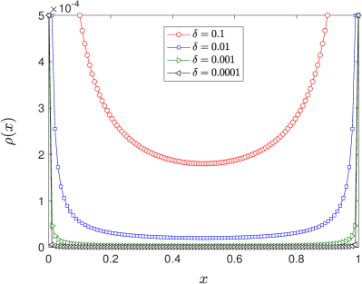
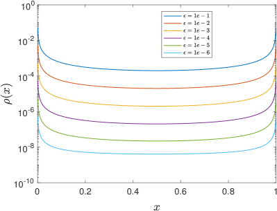
Figure 2: (a) Numerical solution in the bulk ($\rho(x,t)$) at $t=10$ for fixed $\epsilon=1e-3$ and different $\delta$. (b) Numerical solution in the bulk ($\rho(x,t)$) at $t=10$ for fixed $\delta=1e-3$ and different $\epsilon$. $\Delta t=1e-4$ and $h=(1-2\delta)/10^{4}$.

Non-uniform initial condition: In the subsection, we consider a non-uniform initial condition

(69) $$\rho(x)=\begin{cases}&0.5/(1-2\delta),\quad\delta<x<0.5\\ &1.5/(1-2\delta),\quad 0.5<=x<1-\delta\ ,\\ \end{cases}\quad a(0)=b(0)=0.$$

\begin{overpic}[width=208.13574pt]{Non_uniform_bulk_solution_ep_1e-3_delta_1e-3_T_10} \put(0.0,70.0){(a)} \end{overpic}

\begin{overpic}[width=190.79385pt]{Non_uniform_at_bt} \put(-9.0,78.0){(b)} \end{overpic}

\begin{overpic}[width=208.13574pt]{Non_uniform_Energy_ep_1e-3_delta_1e-3} \put(0.0,48.0){(c)} \end{overpic}

\begin{overpic}[width=208.13574pt]{Non_uniform_1-st_moment_ep_1e-3_delta_1e-3} \put(-2.0,48.0){(d)} \end{overpic}

Figure 3: (a) Numerical solution $\rho(x,t)$ at $t=10$. (b) Numerical solution for $a(t)$ and $b(t)$. (c) Evolution of the discrete energy. (d) Evolution of first moment.

Fig. 3(a) shows the numerical solution $\rho(x,t)$ for $\delta=0.001$ and $\epsilon=0.001$ at $t=10$, with $h=10^{-4}$ and $\tau=10^{-4}$. The time evolution of $a(t)$ and $b(t)$ are shown in Fig. 3 (b). The evolution of discrete energy and the 1-st moment are shown in Fig. 3 (c) and (d). In this case, we can also observe the energy stability and the first moment is almost a constant.

Gaussian initial distribution: Last, we take the initial condition as a Gaussian distribution

(70) $$\rho_{0}(x)=\frac{1}{\sqrt{2\pi}\sigma}\exp(-\frac{(x-x_{0})^{2}}{2\sigma^{2}}),\quad a(0)=b(0)=0,$$

with $\sigma=0.1$ and $x_{0}=0.4$. Fig. 4 shows the numerical results for $\delta=1e-4$ and $\epsilon=1e-4$. Fig. 4(a) shows $\rho(x,t)$ for $t=0$, $0.1$, $0.5$ and $2$, respectively, while Fig. 4(b) shows the evolution of $a(t)$ and $b(t)$ with respect to $t$. The evolution of discrete energy and the 1-st moment are shown in Fig. 3 (c) and (d). Again, the numerical scheme is energy stable and 1-st moment is also a constant..

\begin{overpic}[width=208.13574pt]{Gaussian_rho_t_ep_1e-3_delta_1e-3} \put(0.0,70.0){(a)} \end{overpic}

\begin{overpic}[width=190.79385pt]{Gaussian_at_bt_ep_1e-3_delta_1e-3} \put(-9.0,78.0){(b)} \end{overpic}

\begin{overpic}[width=208.13574pt]{Gaussian_Energy_ep_1e-3_delta_1e-3} \put(0.0,48.0){(c)} \end{overpic}

\begin{overpic}[width=208.13574pt]{Gaussian_moment_ep_1e-3_delta_1e-3} \put(-3.0,48.0){(d)} \end{overpic}

Figure 4: (a) Numerical solution $\rho(x,t)$ for different $t$.(b) Numerical solution for $a(t)$ and $b(t)$. (c) Evolution of the discrete energy. (d) Evolution of first moment.

Monotonicity of $a(t)$ and $b(t)$: A crucial assumption in proving the existence of strong solutions is $a^{\prime}(t)\geq 0$ and $b^{\prime}(t)\geq 0$. As discussed earlier, it requires that $\epsilon$ small enough. In this subsection, we present some numerical results show that if $\epsilon$ is not small enough, we may have $a^{\prime}(t)<0$ or $b^{\prime}(t)<0$. To this end, we consider the initial value

(71) $$\rho(x,0)=0.02/(1-2\delta),\quad x\in(\delta,1-\delta),\quad a(0)=b(0)=0.49.$$

Fig. 5 shows $a(t)$ for $t\in(0,0.1)$ for fixed $\delta=10^{-4}$ and different $\epsilon$. One can see that for relative large $\epsilon$, $a(t)$ is not a monotonic function. But interestingly, $a(t)$ will be a monotonic function for $t>t^{*}$ where $t^{*}$ is a time depends on $\epsilon$.

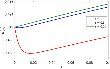
Figure 5: Numerical solution of $a(t)$ for fixed $\delta=10^{-4}$ and different $\epsilon$.

6 Conclusion remark

We proposed a new continuum model for a random genetic drift problem by incorporating a dynamic boundary condition approach. The dynamic boundary condition compensates for singularities on the boundary in the original Kimura equation. We have demonstrated the existence and uniqueness of a strong solution for the regularized system. Finally, we present some numerical results for the regularized model, which indicate that the model can capture the main features of the original model. As future work, we will further study the long-term behavior of the new model. Additionally, we plan to extend current approach to multi-alleles genetic drift problem.

References

- [1] J. A. Carrillo, L. Chen, and Q. Wang, An optimal mass transport method for random genetic drift, SIAM Journal on Numerical Analysis, 60 (2022), pp. 940–969.
- [2] J.-B. Casteras and L. Monsaingeon, Hidden dissipation and convexity for kimura equations, arXiv preprint arXiv:2209.15361, (2022).
- [3] F. A. Chalub, L. Monsaingeon, A. M. Ribeiro, and M. O. Souza, Gradient flow formulations of discrete and continuous evolutionary models: a unifying perspective, Acta Applicandae Mathematicae, 171 (2021), p. 24.
- [4] F. A. Chalub and M. O. Souza, A non-standard evolution problem arising in population genetics, Communications in Mathematical Sciences, 7 (2009), pp. 489–502.
- [5] C. E. Dangerfield, D. Kay, S. Macnamara, and K. Burrage, A boundary preserving numerical algorithm for the wright-fisher model with mutation, BIT Numerical Mathematics, 52 (2012), pp. 283–304.
- [6] C. Duan, C. Liu, C. Wang, and X. Yue, Numerical complete solution for random genetic drift by energetic variational approach, ESAIM: Mathematical Modelling and Numerical Analysis, 53 (2019), pp. 615–634.
- [7] C. L. Epstein and R. Mazzeo, Wright–fisher diffusion in one dimension, SIAM journal on mathematical analysis, 42 (2010), pp. 568–608.
- [8] , Degenerate diffusion operators arising in population biology, no. 185, Princeton University Press, 2013.
- [9] S. N. Ethier and M. F. Norman, Error estimate for the diffusion approximation of the wright–fisher model., Proceedings of the National Academy of Sciences, 74 (1977), pp. 5096–5098.
- [10] L. C. Evans, Partial Differential Equations, vol. 19, American Mathematical Soc., 2010.
- [11] W. J. Ewens, Mathematical population genetics: theoretical introduction, vol. 27, Springer, 2004.
- [12] W. Feller, Diffusion processes in genetics, (1951).
- [13] R. A. Fisher, Xxi.—on the dominance ratio, Proceedings of the royal society of Edinburgh, 42 (1923), pp. 321–341.
- [14] P. A. Jenkins and D. Spano, Exact simulation of the wright–fisher diffusion, (2017).
- [15] M. Kimura, On the probability of fixation of mutant genes in a population, Genetics, 47 (1962), p. 713.
- [16] P. Knopf, K. F. Lam, C. Liu, and S. Metzger, Phase-field dynamics with transfer of materials: the cahn–hilliard equation with reaction rate dependent dynamic boundary conditions, ESAIM: Mathematical Modelling and Numerical Analysis, 55 (2021), pp. 229–282.
- [17] A. N. Kolmogorov, Selected Works of A. N. Kolmogorov: Volume II Probability Theory and Mathematical Statistics, Springer Netherlands, Dordrecht, 1992, ch. Transition of Branching Processes to Diffusion Processes and Related Genetic Problems, pp. 466–469.
- [18] A. McKane and D. Waxman, Singular solutions of the diffusion equation of population genetics, Journal of theoretical biology, 247 (2007), pp. 849–858.
- [19] T. Roubíček, Nonlinear partial differential equations with applications, vol. 153, Springer Science & Business Media, 2013.
- [20] J. Rulla and N. J. Walkington, Optimal rates of convergence for degenerate parabolic problems in two dimensions, SIAM journal on numerical analysis, 33 (1996), pp. 56–67.
- [21] T. D. Tran, J. Hofrichter, and J. Jost, An introduction to the mathematical structure of the wright–fisher model of population genetics, Theory in Biosciences, 132 (2013), pp. 73–82.
- [22] , The free energy method and the wright–fisher model with 2 alleles, Theory in Biosciences, 134 (2015), pp. 83–92.
- [23] W. Walter, On the strong maximum principle for parabolic differential equations, Proceedings of the Edinburgh Mathematical Society, 29 (1986), pp. 93–96.
- [24] Y. Wang and C. Liu, Some recent advances in energetic variational approaches, Entropy, 24 (2022), p. 721.
- [25] Y. Wang, C. Liu, P. Liu, and B. Eisenberg, Field theory of reaction-diffusion: Law of mass action with an energetic variational approach, Physical Review E, 102 (2020), p. 062147.
- [26] S. Wright, Evolution in mendelian populations, Genetics, 16 (1931), p. 97.
- [27] , The differential equation of the distribution of gene frequencies, Proceedings of the National Academy of Sciences, 31 (1945), pp. 382–389.
- [28] S. Xu, M. Chen, C. Liu, R. Zhang, and X. Yue, Behavior of different numerical schemes for random genetic drift, BIT Numerical Mathematics, 59 (2019), pp. 797–821.
- [29] L. Zhao, X. Yue, and D. Waxman, Complete numerical solution of the diffusion equation of random genetic drift, Genetics, 194 (2013), pp. 973–985.