Estimation and Testing of Forecast Rationality
with Many Moments

We in this paper utilize P-GMM (Cheng and Liao,, 2015) moment selection procedure to select valid and relevant moments for estimating and testing forecast rationality under the flexible loss proposed by Elliott et al., (2005). We motivate the moment selection in a large dimensional setting, explain the fundamental mechanism of P-GMM moment selection procedure, and elucidate how to implement it in the context of forecast rationality by allowing the existence of potentially invalid moment conditions. A set of Monte Carlo simulations is conducted to examine the finite sample performance of P-GMM estimation in integrating the information available in instruments into both the estimation and testing, and a real data analysis using data from the Survey of Professional Forecasters issued by the Federal Reserve Bank of Philadelphia is presented to further illustrate the practical value of the suggested methodology. The results indicate that the P-GMM post-selection estimator of forecaster’s attitude is comparable to the oracle estimator by using the available information efficiently. The accompanying power of rationality and symmetry tests utilizing P-GMM estimation would be substantially increased through reducing the influence of uninformative instruments. When a forecast user estimates and tests for rationality of forecasts that have been produced by others such as Greenbook, P-GMM moment selection procedure can assist in
achieving consistent and more efficient outcomes.

Keywords: Forecast rationality, Moment selection, P-GMM, Relevance, Validity.

JEL Classification: C10, C36, C53, E17.

1 Introduction

Forecasting is an essential technique in economics, as well as in statistics and other sciences. From the forecast producer’s perspective, it is critical to understand how to produce optimal forecasts in light of the available information and a loss function. However, from the viewpoint of the forecast user, we are interested in how to estimate and test for rationality of forecasts that have been produced by someone else, typically the government (Greenbook), even if the loss function of the producer of forecasts is unknown. Elliott et al., (2005) (hereafter EKT (2005)) test forecast optimality under general classes of loss functions that nest popular loss functions as special cases (Figure 1), where the family of loss functions is indexed by a single unknown parameter $\alpha$. Such a parameter has significant economic value because it informs forecast user about the forecaster’s objectives. EKT (2005) establish conditions under which this parameter $\alpha$ is identified and further propose a $J$-test for overidentification to test the forecast rationality under asymmetric loss in linear generalized method of moments (GMM) framework.
The loss function they utilize to identify the forecaster’s attitude parameter $\alpha$ is

$$L_{p}\left(e_{t+h};\alpha\right)\equiv\left[\alpha+(1-2\alpha)\mathbb{I}\left(e_{t+h}<0\right)\right]\lvert e_{t+h}\rvert^{p},\vspace{-0.05cm}$$ (1.1)

in which $\mathbb{I}(\cdot)$ represents the indicator function that is equal to unity when the condition $e_{t+h}<0$ holds and zero otherwise, $p$ indicates a positive exponent determining the curvature of the loss function, $\alpha$ denotes an asymmetry parameter with range $0<\alpha<1$, $h\geq 0$ is an integer variable that measures the forecast horizon, and $e_{t+h}$ stands for the forecast error. A positive forecast error results from underestimating the target variable, while a negative forecast error arises out of overestimating it. Therefore, we
refer to $\alpha$ as the forecaster’s attitude parameter.

Figure 1: Loss Function with Different Values of $\alpha$ (Left: $p=2$; Right: $p=1$)

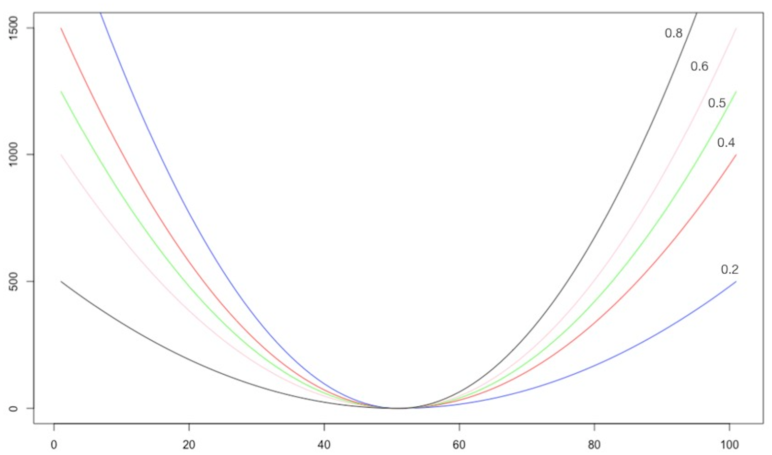
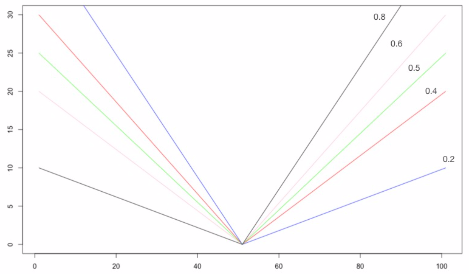
Note: The plot shows how the magnitude of the asymmetric parameter influences the univariate loss functions. It demonstrates that even minor variations in $\alpha$ from the symmetric loss value of 0.5 imply fairly significant loss disparities. For instance, with $\alpha=0.4$, the loss ratio for both positive and negative forecast errors is $\alpha/(1-\alpha)=2/3$, resulting in a loss differential of approximately 33%.

In accordance with the optimization problem (1.1), the appropriate action that forecast producer takes should satisfy the forecast optimality condition

$$\mathbb{E}\left(W_{t}\left[\mathbb{I}\left(e_{t+h}<0\right)-\alpha_{0}\right]\lvert e_{t+h}\rvert^{p_{0}-1}\right)=0,\vspace{-0.05cm}$$ (1.2)

where $\alpha_{0}$ and $p_{0}$ represent the true values of $\alpha$ and $p$, respectively, $W_{t}$ is the information (instrument) set that the forecaster knows at time $t$, and the optimal forecast error follows a martingale difference sequence with respect to the information set at time $t$. However, usually not all of information in $W_{t}$ is accessible to a forecast user. For the purpose of backing out $\alpha,$ according to the orthogonality of marting-
ale differences, we only need an instrument set $V_{t}\subset W_{t},$ satisfying

$$\mathbb{E}\left(V_{t}\left[\mathbb{I}\left(e_{t+h}<0\right)-\alpha_{0}\right]\lvert e_{t+h}\rvert^{p_{0}-1}\right)=0,$$ (1.3)

which is sufficient to identify $\alpha$ even under model misspecification.

The selection of instrument variables $V_{t}$ directly affects the estimation and testing of forecast rationality. When we use the EKT (2005) approach to back out the forecaster’s attitude parameter $\alpha$, we usually utilize a comprehensive set of instrumental variables to approximate all information available to forecast producer. In reality, the information set $V_{t}$ we can access is typically very large and we may also want to consider nonlinear functions of those instruments. For example, if we have 6 potential instruments, the set of instrument choices will consist of $2^{6}-1=63$ alternatives. If we consider nonlinear functions of those instruments, i.e., $f(V_{t})$ and $f(\cdot)$ is a known transform function such as polynomials, the information set will become much larger, which could result in a singular weighting matrix for the GMM estimation of $\alpha$. While in some circumstances the choice of instruments may be driven by economic concerns, in many cases the selection of instruments might be arbitrary. Occasionally, we could even choose the instruments that forecast producer does not use, resulting in biased estimators and misleading inferences. This bias would be larger when the number of moments $d=\dim(V_{t})$ is large. Meanwhile, estimates are often very sensitive to the instruments that we choose. Some instruments may be invalid resulting in inconsistent estimation of $\alpha$, while other instruments may be redundant resulting in additional finite sample bias without bringing any useful information to improve estimation efficiency. Therefore, for consistently and efficiently estimating $\alpha$ and increasing the power of rationality and symmetry tests, it is important to identify the valid and relevant instruments (moment conditions) whenever there is no prior information about their validity. To the best of our knowledge, the EKT (2005) approach has not been combined with any moment selection methods thus far to account for the uncertain validity and relevance of moment conditions in the presence of a large number of potential instruments. The goal of this paper is to identify the instruments that are both valid and rele-
vant to back out the parameter $\alpha$ to learn the forecaster’s preference or/and loss attitude.

A lot of research has been devoted to choosing moment conditions (1.3) in the presence of many possible instruments. Built on a trade-off between the $J$-test statistics and the number of moment conditions, Andrews, (1999) and Andrews and Lu, (2001) put forth a moment selection criterion, which takes the form of the $J$-test statistics of overidentifying restrictions plus a penalty term that accounts for the number of moment conditions, in order to single out a set of valid moment conditions among all possible choices. Hong et al., (2003) develop a model selection criteria for unconditional moment models using generalized empirical likelihood statistics. Liao, (2013) suggests a GMM shrinkage procedure for the selection of valid moment conditions by adding a penalty function to the GMM criterion. Caner et al., (2018) introduce the adaptive elastic net GMM estimator in large-dimensional models with potentially (locally) invalid moment conditions. However, all of the aforementioned research only takes the moment validity into account under the premise that all of the moments are relevant. To effectively select the relevant moment conditions, Andrews, (2002) and Inoue, (2006) utilize a bootstrap setup relying on Edgeworth expansions. Hall et al., (2007) present a moment selection criterion formed on entropy that can be applied to choose relevant moments. Ng and Bai, (2009) propose an $L_{2}$-Boosting methodology for relevant instrument selection. Luo, (2015) puts forward a LASSO based selection procedure using the $L_{1}$ penalty to pick out the informative moments. Larin, (2016) suggests a statistic, which follows a chi-squared limiting distribution when the estimator of moments covariance matrix converges at the rate $\sqrt{T}$, to test the relevance of moment conditions, where $T$ denotes sample size. Nevertheless, each of the above-mentioned approaches is established on the assumption that all candidate
moments are valid, which is evidently an undesirable aspect of any forecast evaluation procedure.

Recently, gleaned from the shrinkage procedure proposed by Liao, (2013), Cheng and Liao, (2015) study the selection of valid and relevant moments using a penalized GMM estimation, where a novel penalty is designed to incorporate information on both moment validity and relevance for adaptive estimation, henceforth referred to as P-GMM estimation. Lee and Xu, (2018) bring forward a selection algorithm named Double-Boosting GMM relied on boosting to choose the valid and relevant instruments from a set of high dimensional instruments and show that their algorithm can give smaller mean squared errors than Cheng and Liao, (2015) in the simulations. Belloni et al., (2018) recommend a regularized GMM to construct moment equations $M(\theta;\eta)=0$ for the target parameter $\theta$ given the nuisance parameter $\eta$ such that the true values of the parameters follow $M\left(\theta_{0};\eta_{0}\right)=0$. Lai et al., (2010) establish an empirical likelihood ratio statistic to eliminate invalid models firstly and then apply bootstrap procedure to choose the model that yields the smallest approximate variance of the estimate. All of these methods could be applied directly to choose the valid and relevant moment conditions simu-
ltaneously for the GMM estimation.

In the EKT (2005) methodology, we typically do not prioritize the estimation of regression coefficients, and there are instances where we lack awareness of the variable types employed by forecast producers. Consequently, traditional methods that focus solely on estimating target coefficients cannot be directly employed to select the valid and relevant moments to identify the forecaster’s attitude parameter $\alpha$. In alignment with this, the approach proposed by Cheng and Liao, (2015), which incorporates a penalty within the standard GMM criterion, can be employed in the framework of EKT (2005) to select moment conditions for the purpose of estimating and testing forecast rationality under flexible loss functions. Particularly, we demonstrate that P-GMM technique enjoys moment selection consistency and is able to select all valid and relevant moment conditions without restricting the forecast user’s knowledge of any particular information sets, which simultaneously provides more efficient post-selection estimation. Asymptotically, the resultant P-GMM post-selection estimator of forecaster’s attitude enjoys oracle property under consistent moment selection, i.e., as efficient as the oracle GMM
estimator formulated on all valid and relevant moment conditions.

To shed light on the statistical properties of P-GMM estimation of forecast rationality, we undertake a set of Monte Carlo simulations, including both linear and nonlinear dependencies between the forecast user’s information set and the forecast error. The Monte Carlo simulation results indicate that P-GMM procedure could provide an unbiased and more efficient estimator of $\alpha$ compared to the case where we deploy all (valid) moment conditions. The suggested P-GMM estimation is appealing since the obtained post-selection outcomes can be comparable to the oracle estimators by using the available information efficiently. In addition, P-GMM estimation has the potential to enhance the estimator by reducing its standard error and increase the power of $J$-test statistics by mitigating the influence of irrelevant instruments. These findings further demonstrate that even if forecast user does not have any information regarding the validity of instrumental variables in practice, P-GMM estimation can be extremely helpful with relevance to select moment conditions in the context of EKT (2005) for producing consistent and more efficient results. We then apply the suggested P-GMM estimation to data from the Survey of Professional Forecasters issued by the Federal Reserve Bank of Philadelphia to further elucidate its practical value. The empirical results highlight the necessity of undertaking moment selection.

The outline of this paper is as follows. Section 2 provides a brief review of EKT (2005) method for testing forecast rationality and motivates moment selection issue that inspires the development of the suggested estimation procedure. Section 3, built on the P-GMM estimation method, selects valid and relevant moment conditions within the framework of EKT (2005), for which the moment selection consistency is presented. Section 4 includes simulation examples to shed light on the statistical properties of the developed estimation and testing of forecast rationality. Section 5 presents a real data analysis using data from the Survey of Professional Forecasters to further illustrate the performance of the
suggested P-GMM estimation. We conclude this paper in Section 6.

2 Estimation and Testing of Forecast Rationality: EKT (2005)

According to the setup of EKT (2005), $X\equiv\left\{X_{t}:\Omega\rightarrow\mathbb{R}^{m+1},m\in\mathbb{N},t=1,\dots,T\right\}$ is a stochastic process defined on a complete probability space $(\Omega,\mathcal{F},P)$, where $\mathcal{F}=\left\{\mathcal{F}_{t},t=1,\dots,T\right\}$ and $\mathcal{F}_{t}$ is the $\sigma$-field generated by $\mathcal{F}_{t}\equiv\sigma\left\{X_{s},s\leqslant t\right\}$. In addition, $Y_{t}$ is the continuous component of interest of the observed vector $X_{t}$ with distribution function $F_{t}(\cdot)$ conditional on the information set $\mathcal{F}_{t}$. The forecasting problem is hence to predict the value of $Y_{t+h}$ by $f_{t+h}\equiv\theta^{\prime}W_{t}$ dependent upon the information set $\mathcal{F}_{t}$, in which $\theta$ is an unknown vector of parameters, $W_{t}$ is a vector of variables that are $\mathcal{F}_{t}$-measurable, and $Z^{\prime}$ represents the transpose of a matrix or vector $Z$. A generalized loss function $L(\cdot)$, which is a
mapping from realizations and forecasts to the real line, is defined as

$$L(p,\alpha,\theta)\equiv\left[\alpha+(1-2\alpha)\mathbb{I}\left(Y_{t+h}-f_{t+h}<0\right)\right]\lvert Y_{t+h}-f_{t+h}\rvert^{p},\vspace{-0.05cm}$$ (2.1)

where $Y_{t+h}-f_{t+h}$ represents the forecast error $e_{t+h}$. For easy calculations, EKT (2005) assume that the value of the loss shape parameter $p_{0}$ is known and deliberate on the estimation of forecaster’s attitude parameter $\alpha$. Given $p_{0}$ and $\alpha_{0}$, the $h$-step-ahead forecast of $Y_{t+h}$, $f_{t+h}^{*}=\theta^{*\prime}W_{t}$, is rational if $\theta^{*}=$
$\arg\min_{\theta\in\Theta}$ $\mathbb{E}\left\{L\left(\alpha_{0},p_{0},\theta\right)\right\}$, which solves the following moment condition

$$\mathbb{E}\left(W_{t}\left[\mathbb{I}\left(Y_{t+h}-f_{t+h}^{*}<0\right)-\alpha_{0}\right]\lvert Y_{t+h}-f_{t+h}^{*}\rvert^{p_{0}-1}\right)=0.$$ (2.2)

In order to back out $\alpha$, the first order condition of (2.1) should hold if and only if $\alpha=\alpha_{0}$. As specified by $Proposition$ 1 in EKT (2005), we recognize that the solution $f_{t+1}^{*}$ is exclusive, which indicates that the forecaster’s attitude parameter $\alpha$ is unique even under model misspecification. Note that (2.2) can be considered as a moment condition $\mathbb{E}\left[W_{t}\left(\mathbb{I}\left(e_{t+h}^{*}<0\right)-\alpha_{0}\right)\lvert e_{t+h}^{*}\rvert^{p_{0}-1}\right]=0$, where $e_{t+h}^{*}\equiv Y_{t+h}-f_{t+h}^{*}=Y_{t+h}-\theta^{*\prime}W_{t}$ is the forecast error given $f^{*}_{t+h}$. It suggests that if the forecasts are optimal, then any information $W_{t}$ must be correctly included in $f_{t+h}^{*}$, so that $W_{t}\left(\mathbb{I}\left(e_{t+h}^{*}<0\right)-\alpha_{0}\right)$ is orthogonal to the forecast errors. For a given $f_{t+h}^{*}$, we can back out $\alpha_{0}$ using this moment condition as well. In reality, not all variables in $W_{t}$ are known to the forecast user. Supposing that the user of forecast obs-
erves a $d$-vector variables $V_{t}$, which is a subvector of $W_{t}$, we would have

$$\mathbb{E}(V_{t}[\mathbb{I}(Y_{t+h}-f_{t+h}^{*}<0)-\alpha_{0}]\lvert Y_{t+h}-f_{t+h}^{*}\rvert^{p_{0}-1})=\mathbb{E}(C_{t}-\alpha_{0}B_{t})=0,$$ (2.3)

where $C_{t}=V_{t}\mathbb{I}(Y_{t+h}-f_{t+h}^{*}<0)\lvert Y_{t+h}-f_{t+h}^{*}\rvert^{p_{0}-1}$ and $B_{t}=V_{t}\lvert Y_{t+h}-f_{t+h}^{*}\rvert^{p_{0}-1}$. Thenceforth, $\alpha_{0}$ can
be solved by minimizing the quadratic norm of (2.3)

$$\min_{\alpha}Q(\alpha)=\mathbb{E}(C_{t}-\alpha B_{t})^{\prime}S^{-1}\mathbb{E}(C_{t}-\alpha B_{t}),\vspace{-0.025cm}$$ (2.4)

in which $S=\mathbb{E}((C_{t}-\alpha B_{t})(C_{t}-\alpha B_{t})^{\prime})=\mathbb{E}[V_{t}V_{t}^{\prime}\left(\mathbb{I}\left(Y_{t+h}-f_{t+h}^{*}<0\right)-\alpha_{0}\right)^{2}\lvert Y_{t+h}-f_{t+h}^{*}\rvert^{2p_{0}-2}]$ is a
positive definite weighting matrix. Taking derivative of (2.4) with respect to $\alpha$, we achieve

$$\alpha_{0}=\arg\min_{\alpha}Q(\alpha)=[\mathbb{E}(B_{t}^{\prime}S^{-1}B_{t})]^{-1}\mathbb{E}(B_{t}^{\prime}S^{-1}C_{t}).\vspace{-0.025cm}$$ (2.5)

Given a sample path of instrument vectors $\left(V_{1}^{\prime},\ldots,V_{T}^{\prime}\right)^{\prime}$ with $T$ observations, we obtain the esti-
mator of $\alpha_{0}$ from the empirical mean of (2.5)

$$\hat{\alpha}_{T}=(\hat{B}_{T}^{\prime}\hat{S}_{T}^{-1}\hat{B}_{T})^{-1}(\hat{B}_{T}^{\prime}\hat{S}_{T}^{-1}\hat{C}_{T}),$$ (2.6)

where $\hat{B}_{T}=1/T\sum_{t=1}^{T}V_{t}\lvert Y_{t+h}-{f}^{*}_{t+h}\rvert^{p_{0}-1}$, $\hat{C}_{T}={1}/{T}\sum_{t=1}^{T}V_{t}\mathbb{I}(Y_{t+h}-{f}^{*}_{t+h}<0)\lvert Y_{t+h}-{f}^{*}_{t+h}\rvert^{p_{0}-1}$, and $\hat{S}_{T}\equiv{1}/{T}\sum_{t=1}^{T}[V_{t}V_{t}^{\prime}\left(\mathbb{I}\left(Y_{t+h}-f_{t+h}^{*}<0\right)-\hat{\alpha}_{T}\right)^{2}\lvert Y_{t+h}-f_{t+h}^{*}\rvert^{2p_{0}-2}]$ is a consistent estimate of $S$. Both $\hat{\alpha}_{T}$ and $\hat{S}_{T}$ can be solved by iteration, where we first choose a preliminary weighting matrix $\hat{S}_{T}=I_{d\times d}$ (Newey and West,, 1987). Up to now, we can see that the instrument validity is pretty important as it affects the estimate of $\alpha$ through all factors appearing in (2.6). Indeed, each set of instruments would generate different estimate and asymptotic variance, and only the inclusion of all the available information would produce an efficient estimator $\hat{\alpha}_{T}$. Nevertheless, in practical applications, the forecast user sometimes is unable to determine which instrumental variable is valid. It is necessary for us to int-
roduce an estimation procedure for assessing instrument validity and avoiding estimation bias.

After that, we have asymptotic normality (EKT (2005) $Proposition$ 4) given $p_{0}=1$ or 2 when the
true value of $\alpha$ is in the interior of the parameter space,

$$T^{\frac{1}{2}}\left(\hat{\alpha}_{T}-\alpha_{0}\right)\stackrel{{\scriptstyle d}}{{\rightarrow}}\mathcal{N}(0,\left(B^{\prime}S^{-1}B)^{-1}\right)$$ (2.7)

with $B=\mathbb{E}(B_{t})$, which can be utilized to test whether $\hat{\alpha}_{T}$ differs from $\alpha_{0}$. In practice, we can simulate the asymptotic distribution of the $\alpha$ estimate according to Andrews, (2002) if the true value of $\alpha$ is on the boundary of the parameter space. Regarding rationality test (EKT (2005) $Corollary$ 5), a joint null hypothesis of forecast rationality and the flexible loss function can be conducted with $d>1$ instru-
ments through the test statistic for overidentification

$$J_{T}\left(\hat{\alpha}_{T}\right)=T\times\hat{Q}_{T}\left(\hat{\alpha}_{T}\right)=T\times\hat{A}_{T}\left(\hat{\alpha}_{T}\right)^{\prime}\hat{S}_{T}^{-1}\left(\hat{\alpha}_{T}\right)\hat{A}_{T}\left(\hat{\alpha}_{T}\right)\sim\chi_{d-1}^{2},$$ (2.8)

where $\hat{A}_{T}\left(\hat{\alpha}_{T}\right)=\hat{C}_{T}-\hat{\alpha}_{T}\hat{B}_{T}$ and a large value of the $J_{T}(\hat{\alpha}_{T})$ indicates the rejection of forecast rationality. If there is only one instrumental variable available and overidentification cannot be tested as a result, a unique closed form solution for estimator $\hat{\alpha}_{T}$ exists. For testing loss symmetry, with a fixed
value $\hat{\alpha}_{T}=0.5$, we have

$$J_{T}\left(0.5\right)=T\times\hat{Q}_{T}\left(0.5\right)=T\times\hat{A}_{T}\left(0.5\right)^{\prime}\hat{S}_{T}^{-1}\left(\hat{\alpha}_{T}\right)\hat{A}_{T}\left(0.5\right)\sim\chi_{d}^{2},\vspace{-0.025cm}$$ (2.9)

in which the degrees of freedom equals to $d$ as there is no parameter needing to be estimated. The rejection of this test would indicate the refusal of the loss symmetry if (2.8) is not disregarded. The conditional distribution of (2.9) is difficult to obtain. Following Wang and Lee, (2014), we interpret $J_{T}(0.5)$ as a test for loss symmetry after we select all valid and relevant moment conditions. The aforementioned discussions reveal that the reliability of the moment conditions has a significant impact on the statistical features of the GMM estimator $\hat{\alpha}_{T}$. It would be beneficial to incorporate information on
both moment validity and relevance for rationality and symmetry tests.

Remark 2.1.

There is a strong assumption in EKT (2005) that the forecasts are generated using a linear model $f_{t+h}=\theta^{\prime}W_{t}$. In case of the nonlinear model, where $f_{t+h}=f(\theta,W_{t})$ and $f(\cdot)$ is continuously
differentiable, there exists $\theta^{*}$ that satisfies

$$\mathbb{E}\big{(}f^{*}_{t+h}\big{[}\mathbb{I}\big{(}Y_{t+h}-f_{t+h}^{*}<0\big{)}-\alpha_{0}\big{]}\lvert Y_{t+h}-f_{t+h}^{*}\rvert^{p_{0}-1}\big{)}=0,$$

where $f^{*}_{t+h}=f(\theta^{*},W_{t})$. Accordingly, we can utilize $V_{v,t}$, which is a subvector of $f^{*}(\theta^{*},W_{t})$, to conduct the rationality test. The point is that for the nonlinear case, $f^{*}(\theta^{*},W_{t})$ will be dependent on both $\theta^{*}$ and $W_{t}$, but in reality we do not know the value of $\theta^{*}$ which forecast user employs; see Naghi, (2014) for
further discussion. Consequently, we in this paper only concentrate on the linear relationship.

The EKT (2005) method takes into consideration asymmetric preferences and offers the most latitude in terms of the loss function among the tests of prediction optimality that are currently available in the literature. Nonetheless, one of the fundamental assumptions implicitly underlying the EKT (2005) is that the forecast user has a full picture of available information, as reflected by (2.2). In practical applications, (2.3) is extremely useful since forecast user cannot achieve all information that forecasters have access to. However, even given the instrument set $V_{t}$, it is still unclear how the forecasting institutions incorporate the information available in $V_{t}$ to improve the forecast and how we should select the instruments to reach the most efficient value of $\alpha$, since for each element of $V_{t}$, we could obtain an estimate for $\alpha_{0}$ that would rationalize the observed sequence of forecasts. EKT (2005) suggest applying data-based methods for the selection of moment conditions using criteria such as those put forward by Donald and Newey, (2001), where they look into how to identify instruments from a subset that is known to be valid. Such a data-based method is useful when dealing with a limited and fixed number of moment conditions. The problem is that in reality we may have many instruments or moment conditions, and we cannot guarantee that all instruments we are planning to select are valid. If the used instruments do not belong to the original information set, the forecast rationality estimation and testing could lead to misleading inferences. We have to conduct some judgements for valid instruments before we carry on the relevance selection, which is the primary problem this paper explores. To estimate and test forecast rationality under the flexible loss acquired from EKT (2005), we adopt P-GMM estima-
tion method to select all valid and relevant instruments.

3 Moment Selection by P-GMM: Validity and Relevance

The estimation and testing of forecast rationality under flexible loss is a crucial issue of considerable interest for forecast users from both theoretical and empirical perspectives. If the forecasts do not efficiently use the information in $V_{t}$, then the estimator of $\alpha$ would be very different for each of the moment conditions and the test for overidentification would reject. Nonetheless, in empirical applications, there are no general rules for choosing instruments. How to select the suitable (valid and relevant) instruments to back out the forecaster’s attitude parameter and improve estimation efficiency is still not clear in the context of EKT (2005). To motivate the methodology suggested in this paper, suppose th-
ere is a set of possibly misspecified moment conditions

$$\mathbb{E}\left(V_{t}\left[\mathbb{I}\left(Y_{t+h}-f_{t+h}^{*}<0\right)-\alpha_{0}\right]\lvert Y_{t+h}-f_{t+h}^{*}\rvert^{p_{0}-1}\right)\overset{?}{=}0\vspace{-0.07cm}$$ (3.1)

with instruments $V_{t}$, where “$\overset{?}{=}$” represents that equality may hold for some moments but not others. Subsequently, including these misspecified moment conditions in estimating will lead to inconsistent estimation. To address this issue, we employ P-GMM estimation method (Cheng and Liao,, 2015), which can select valid and relevant moment conditions simultaneously to obtain not only an unbiased but also
a more efficient estimator of $\alpha$ (Figure 2).

Practically, (2.3) is the primary equation we need to utilize to select valid moment conditions, which implies that if an instrument does not satisfy (2.3), we cannot adopt it to carry on the estimation. After that, the relevant instruments are picked up from the valid ones by comparing the variance of estimators. If a set of moment conditions yields a smaller variance, indicating that more information becomes available, this set of moment conditions will be treated as relevant moments, for which $(B^{\prime}S^{-1}B)^{-1}$ is the main indicator we concentrate on. These two selection steps are the crucial points that many papers have emphasized for instrument or moment selection; see Lai et al., (2010). P-GMM estimation combines these two selection steps together by attaching an appropriate penalty to the standard GMM criterion. Before introducing P-GMM estimation under the framework of EKT (2005), we
provide the definitions of valid and relevant instruments this paper employs.

Definition 1.

(Validity) An instrument $V_{i,t}$ is claimed as a valid instrument in terms of the estimation
of $\alpha$ if and only if it satisfies (2.3), i.e., $\mathbb{E}\left[V_{i,t}\left(\mathbb{I}\left(e_{t+h}^{*}<0\right)-\alpha_{0}\right)\lvert e_{t+h}^{*}\rvert^{p_{0}-1}\right]=0.$

Definition 2.

(Relevancy) A valid instrument $V_{j,t}$ is said to be a relevant instrument in terms of the estimation of $\alpha$ given moment condition $\mathbb{E}\left[(V_{j,t},V_{i,t})^{\prime}\left(\mathbb{I}\left(e_{t+h}^{*}<0\right)-\alpha_{0}\right)\lvert e_{t+h}^{*}\rvert^{p_{0}-1}\right]=0$ if and only
if $\hat{B}^{\prime}_{T}(V_{j,t},V_{i,t})\hat{S}^{-1}_{T}(V_{j,t},V_{i,t})\hat{B}_{T}(V_{j,t},V_{i,t})\geq\hat{B}^{\prime}_{T}(V_{i,t})\hat{S}^{-1}_{T}(V_{i,t})\hat{B}_{T}(V_{i,t}).$

Figure 2: The Roadmap of Instrument Selection

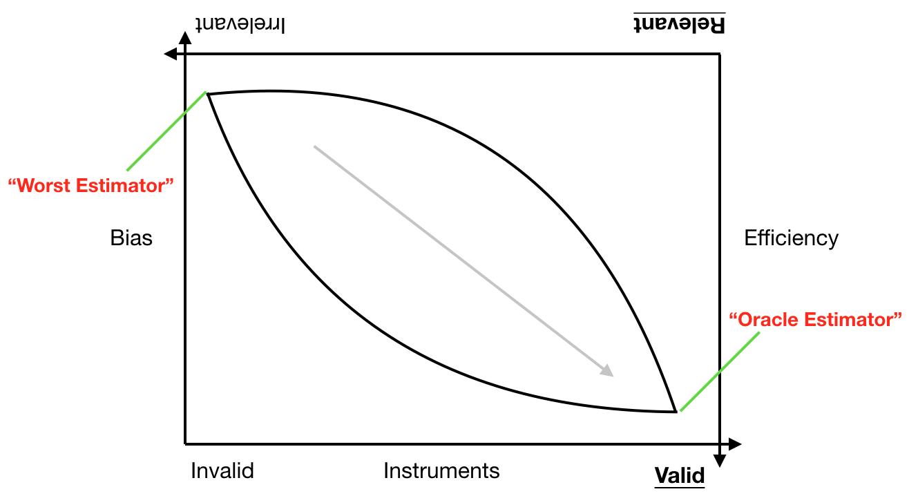
Note: The instruments could be divided into four types: valid and invalid, relevant and irrelevant. To reduce bias, valid instruments must be selected. For obtaining efficiency, relevant instruments should be chosen. To get the unbiased and efficient estimation of the forecaster’s attitude parameter $\alpha$, we need to choose valid and relevant instruments, which is close to “Oracle Estimator”.

Given $\dim(V_{t})=d$, we divide the instrument set $V_{t}$ into categories of “Good” instruments and
“Doubt” instruments, i.e., $V_{t}=(V_{G,t},V_{D,t})^{\prime}$ with $V_{G,t}\in\mathbb{R}^{k_{0}}$ and $V_{D,t}\in\mathbb{R}^{d-k_{0}}$. We assume that a subvector of “Good” moment function $g_{G}(V_{G,t},\alpha)=C_{G,t}-\alpha B_{G,t}\in\mathbb{R}^{k_{0}}$ with $k_{0}<d$, where $C_{G,t}=V_{G,t}$ $\mathbb{I}(Y_{t+h}-f_{t+h}^{*}<0)\lvert Y_{t+h}-f_{t+h}^{*}\rvert^{p_{0}-1}$ and $B_{G,t}=V_{G,t}\lvert Y_{t+h}-f_{t+h}^{*}\rvert^{p_{0}-1}$, can be utilized without testing validity and relevance for the identification of parameter $\alpha$. For instance, the value of $k_{0}$ could be 2, which means $V_{G,t}=(1,Y_{t-1})^{\prime}$, as the constant and lagged dependent variable are well-known valid and relevant instruments. To produce the most substantial collection of valid and relevant moment conditions, following Cheng and Liao, (2015), we adopt $g_{D}(V_{D,t},\alpha)=C_{D,t}-\alpha B_{D,t}\in\mathbb{R}^{d-k_{0}}$ to represent all “Doubt” moment conditions that needing to be checked for validity and/or relevance, where $C_{D,t}=$
$V_{D,t}\mathbb{I}(Y_{t+h}-f_{t+h}^{*}<0)\lvert Y_{t+h}-f_{t+h}^{*}\rvert^{p_{0}-1}$ and $B_{D,t}=V_{D,t}\lvert Y_{t+h}-f_{t+h}^{*}\rvert^{p_{0}-1}$. Correspondingly, $g(V_{t},\alpha)=$
$C_{t}-\alpha B_{t}=[g_{G}(V_{G,t},\alpha),g_{D}(V_{D,t},\alpha)]^{\prime}\in\mathbb{R}^{d}$ denotes the both “Good” and “Doubt” sets of all available moments. For the purpose of choosing moments, a slackness parameter $\beta$ is defined as $\beta=$ $\mathbb{E}[g_{D}(V_{D,t},\alpha)]$. In concert with the preceding definitions of valid and relevant instruments, P-GMM estimation introduces the slackness parameter $\beta_{0}$ into (2.3) to get

$$\mathbb{E}\left(V_{t}\left[\mathbb{I}\left(Y_{t+h}-f_{t+h}^{*}<0\right)-\alpha_{0}\right]\lvert Y_{t+h}-f_{t+h}^{*}\rvert^{p_{0}-1}-\begin{bmatrix}0\\ \beta_{0}\end{bmatrix}\right)\equiv\mathbb{E}\begin{bmatrix}g_{G}(V_{G,t},\alpha_{0})\\ g_{D}(V_{D,t},\alpha_{0})-\beta_{0}\end{bmatrix}=0,$$ (3.2)

where $\beta_{0}=\mathbb{E}[g_{D}(V_{D,t},\alpha_{0})]$. Subsequently, instrument is selected from set ${D}=\mathcal{A}\cup\mathcal{B}_{1}\cup\mathcal{B}_{0}$ with the cardinality $\lvert{D}\rvert=d-k_{0}$, in which $\mathcal{A}$ represents the set of valid and relevant moments, $\mathcal{B}_{0}$ indicates the set of valid but irrelevant ones, and $\mathcal{B}_{1}$ is the set of invalid moments. Both the moments in set $\mathcal{A}$ and $\mathcal{B}_{0}$ are valid, but only those in $\mathcal{A}$ are relevant. We can simultaneously identify $\alpha$ and $\beta$ and attain their joint estimation through (3.2). The efficient estimation and moment selection are achieved in P-GMM esti-
mation by minimizing the following penalized objective function

$${\hat{\alpha}}_{0}=\underset{\alpha}{\arg\min}\Big{[}{\overline{g}_{T}}(\alpha,\beta)^{\prime}S^{-1}_{T}{\overline{g}_{T}}(\alpha,\beta)+\lambda_{T}\sum_{\ell\in\mathcal{A}\cup\mathcal{B}_{1}\cup\mathcal{B}_{0}}\omega_{T,\ell}\lvert\beta_{\ell}\rvert\Big{]},\vspace{-0.1cm}$$ (3.3)

where $\overline{g}_{T}(\alpha,\beta)=\frac{1}{T}\sum_{t=1}^{T}[g_{G}(V_{G,t},\alpha),g_{D}(V_{D,t},\alpha)-\beta]^{\prime}$, $S_{T}$ denotes a symmetric weighting matrix, $\lambda_{T}$ indicates a tuning parameter that regulates the overall penalty level, $\omega_{T,\ell}$ stands for an information-based adaptive adjustment which equals $\dot{\mu}_{T,\ell}^{r_{1}}\lvert\dot{\beta}_{T,\ell}\rvert^{-r_{2}}$, $\dot{\mu}_{T,\ell}$ is an empirical measure of the information in moment $\ell\in{D}$ defined below in (3.4), $\dot{\beta}_{T,\ell}$ represents a preliminary consistent estimator of ${\beta}_{0,\ell}=$
$\mathbb{E}[g_{D}(V_{D,t,\ell},\alpha_{0})]$, and $r_{1}$ and $r_{2}$ are positive constants ($r_{2}\leq r_{1}$ ) that are selected by the forecast user to ensure a small value of $\omega_{T,\ell}$ when the moment condition is irrelevant. Notice that (3.3) is indeed a
LASSO type estimator—each individual slackness parameter $\beta_{\ell}$ is penalized using its $L_{1}$-norm.

Remark 3.1.

To distinguish between valid moments and invalid ones (Definition 1), $\dot{\beta}_{T,\ell}$ plays a dominant role. For valid moments, $\dot{\beta}_{T,\ell}$ will exhibit a reduced magnitude, resulting in a substantial penalty, whereas for invalid moments, $\dot{\beta}_{T,\ell}$ will be larger to lead to a small penalty. We must take into account empirical measure of the information to make the distinction between relevant and irrelevant moments (Definition 2). For relevant moments, $\dot{\mu}_{T,\ell}$ will be larger to lead $\beta$ to zero, while for irrelevant ones,
$\dot{\mu}_{T,\ell}$ will be asymptotically zero, resulting in small shrinkage.

The parameter $\dot{\mu}_{T,\ell}$ in the expression of $\omega_{T,\ell}$ can be chosen by the relevance criteria

$$\dot{\mu}_{T,\ell}=\rho_{\max}\big{(}\hat{B}^{\prime}_{G+\ell}\hat{S}^{-1}_{G+\ell}\hat{B}_{G+\ell}-\hat{B}^{\prime}_{G}\hat{S}^{-1}_{G}\hat{B}_{G}\big{)},\ \ell\in{D}=\mathcal{A}\cup\mathcal{B}_{1}\cup\mathcal{B}_{0},\vspace{-0.05cm}$$ (3.4)

in which $\hat{B}_{G}$ and $\hat{S}_{G}$ are the corresponding estimates defined in the same way as $\hat{B}_{T}$ and $\hat{S}_{T}$ in Section 2, $\rho_{\max}$ denotes the largest difference between $\hat{B}^{\prime}_{G+\ell}\hat{S}^{-1}_{G+\ell}\hat{B}_{G+\ell}$ and $\hat{B}^{\prime}_{G}\hat{S}^{-1}_{G}\hat{B}_{G}$, $(\hat{B}^{\prime}_{G}\hat{S}^{-1}_{G}\hat{B}_{G})^{-1}$ depicts the asymptotic variance of the optimal estimator of $\alpha_{0}$, and $(\hat{B}^{\prime}_{G+\ell}\hat{S}^{-1}_{G+\ell}\hat{B}_{G+\ell})^{-1}$ represents the asymptotic variance of the optimal estimator of $\alpha_{0}$ after adding moment condition $\ell$. According to $Lemma$ 2.1 in Cheng and Liao, (2015), we have $\hat{B}^{\prime}_{G+\ell}\hat{S}^{-1}_{G+\ell}\hat{B}_{G+\ell}\geq\hat{B}^{\prime}_{G}\hat{S}^{-1}_{G}\hat{B}_{G}$, which indicates that adding a
valid moment condition will not decrease the efficiency of the P-GMM post-selection estimator.

The initial estimator of $\dot{\alpha}_{T}$ and $\dot{\beta}_{T,\ell}$ can be estimated by setting $\lambda_{T}=0$ in (3.3). Thereafter, the value of $\dot{\mu}_{T,\ell}$ could be obtained from (3.4). The tuning parameter $\lambda_{T}$ for the $\ell$th moment condition is
calculated by using the explicit formula below

$$\hat{\lambda}_{T,\ell}=2\big{\|}\hat{S}_{T}^{-\frac{1}{2}}(\ell)\widehat{\Pi}_{T}\big{\|}d^{\frac{r_{2}}{4}}T^{-\frac{1}{2}-\frac{r_{2}}{4}},\vspace{-0.035cm}$$ (3.5)

where $\|\cdot\|$ represents the Euclidean norm, $\hat{S}_{T}^{-1}(\ell)$ denotes the $\ell$th row of the matrix $\hat{S}_{T}^{-1}$, $\widehat{\Pi}_{T}$ is the esti-
mator of $\Pi_{T}=I_{d}-S_{T}^{-\frac{1}{2}}\Gamma_{\alpha}\left(\Gamma_{\alpha}^{\prime}S^{-1}_{T}\Gamma_{\alpha}\right)^{-1}\Gamma_{\alpha}^{\prime}S_{T}^{-\frac{1}{2}}$, and $\Gamma_{\alpha}$ indicates the first derivative of $\overline{g}_{T}(\alpha,\beta)$.

We then obtain the main result of this paper—the selection consistency, mainly coming from the $L_{1}$ penalty in (3.3). Asymptotically, within the framework of EKT (2005), P-GMM estimation can correctly estimate that all nonzero parameters ${\beta}_{\ell}$ in sets $\mathcal{B}_{0}$ and $\mathcal{B}_{1}$ as nonzero, whereas all zero parameters in set $\mathcal{A}$ as zero. Therefore, moment selection consistency is achieved by synchronically selecting all valid and relevant moment conditions and automatically excluding all invalid or irrelevant ones.

Theorem 1.

Let $\hat{\beta}_{\ell}$ denote the estimator of the slackness parameter indexed by $\ell$ from (3.3). Built on
the conditions and theorems in Cheng and Liao, (2015), we can acquire the following results

$$\operatorname{P}\left(\cup_{\ell\in\mathcal{B}_{1}}\left\{\hat{\beta}_{\ell}=0\right\}\right)\rightarrow 0\ \text{ as }T\rightarrow\infty\quad\text{(Invalid)},\vspace{-0.05cm}$$

$$\operatorname{P}\left(\cup_{\ell\in\mathcal{B}_{0}}\left\{\hat{\beta}_{\ell}=0\right\}\right)\rightarrow 0\ \text{ as }T\rightarrow\infty\quad\text{ (Irrelevant)},$$

$$\operatorname{P}\left(\cap_{\ell\in\mathcal{A}}\left\{\hat{\beta}_{\ell}=0\right\}\right)\rightarrow 1\ \text{ as }T\rightarrow\infty\quad\text{(Valid and Relevant)}.$$

The detailed proof of Theorem 1 can follow Cheng and Liao, (2015), which is omitted here. The above results reveal that the valid and relevant moments can be distinguished from the invalid or irrelevant ones with a probability tending towards one. It is commonly established that increasing the number of valid instruments will enhance efficiency in the standard GMM setup. Thus, P-GMM can select all valid and relevant moment conditions in the context of EKT (2005) and simultaneously provides a more efficient estimator of $\alpha$, reflected by a smaller standard error. Note that under consistent moment selection, the asymptotic distribution of the P-GMM post-selection estimator $\hat{\alpha}_{0}$ is normal with mean zero, which corresponds to the expression in (2.7) using the asymptotic laws in GMM theory. Such a post-selection estimator could be as efficient as the oracle GMM estimator established on all valid and relevant moment conditions, demonstrating by the simulations shown below. This oracle property indicates that the suggested P-GMM estimation can increase the power of rationality and symmetry tests
through limiting the impact of uninformative instruments.

4 Monte Carlo Simulations

We conduct simulation experiments to illustrate the finite sample properties of the suggested P-GMM estimation within the scope of EKT (2005), including linear dependence and nonlinear dependence between the forecast user’s information set and the forecast error. For both simulation settings, we treat the constant instrument in the valid and relevant set $V_{G,t}$ defined in Section 3. Throughout the whole section, the identity matrix is employed as a weighting matrix in the GMM optimization since it does not require the estimation of any parameters, and the forecast horizon is limited to $h=1$. We explore the behaviour of the estimator of $\alpha$ and investigate the characteristics of the $J$-test statistics to empha-
size the impact of the selection of instrumental variables.

DGP 1: Linear Case  To capture large dimension in the underlying data, we in this simulation let the number of instruments $V_{t}$ be $d=30$. We then generate the random samples from the following data generating process (DGP)

$$Y_{t+1}=\theta_{0}+W_{1,t}\theta_{1}+W_{2,t}\theta_{2}+U_{t},\vspace{-0.15cm}$$ (4.1)

where $Y$ represents the dependent variable, $W_{1}$ and $W_{2}$ are two covariates, $U$ denotes the error term, and the parameters are set to be $\theta_{0}=1$, $\theta_{1}=0.4$, and $\theta_{2}=0.4$. The parameters we choose here are strong enough for identification. The results in Cheng and Liao, (2015) indicate that when we have a weak identification issue, P-GMM estimation is robust at choosing all valid instruments but will select more irrelevant instruments in the finite sample situation. When we increase the sample size, the probability of identifying irrelevant instruments will decrease significantly even in the weak identification case (see Table 2). Because of this, for the estimation part of this simulation study, we only draw attention to the strong identification case. To highlight the effect of invalid instruments, the whole simulated instrument set needs to include a valid but irrelevant instrument vector $W_{v,t}$ and an invalid instrument vector $W_{inv,t}$. For ensuring this, the samples are generated through the following multiva-
riate normal distribution

$$\quad\quad\quad\quad\quad\left(\begin{array}[]{c}{W_{1,t}}\\ {W_{2,t}}\\ {W_{v,t}}\\ {W^{*}_{v,t}}\\ {U_{t}}\end{array}\right)\sim N\left(0,\left(\begin{array}[]{ccccccccc}{1}&{0.2}&{0}&{0}&{0}\\ {0.2}&{1}&{0}&{0}&{0}\\ {0}&{0}&{I_{14}}&{0}&{0}\\ {0}&{0}&{0}&{I_{14}}&{0}\\ {0}&{0}&{0}&{0}&{1}\end{array}\right)\right),$$

$$W_{inv,t}(\ell)=W^{*}_{v,t}(\ell)+c_{\ell}\times U_{t},\ \text{and}\ c_{\ell}=c_{0}+\frac{(\ell-1)\left(\overline{c}-c_{0}\right)}{d/2-1},\ \ell=1,\dots,d-k_{0}$$

with $k_{0}=3$ for $V_{G,t}=(1,W_{1,t},W_{2,t})^{\prime}$, where $W_{inv,t}(\ell)$ and $W^{*}_{v,t}(\ell)$ are the $\ell$th instruments. Since $W_{inv,t}(\ell)$ is correlated with $U_{t}$, it is evident that the set of instruments used for estimating and testing
forecast rationality does not encompass it.

DGP 2: Nonlinear Case  For this simulation, we consider $d=31$ with nonlinear dependence. We generate the random samples from the following nonlinear DGP

$$Y_{t+1}=\theta_{0}+W^{2}_{1,t}\theta_{1}+(W_{1,t}\times W_{2,t})\theta_{2}+\exp(W_{3,t})\theta_{3}+U_{t},\vspace{-0.12cm}$$ (4.2)

where $\theta_{0}=1$, $\theta_{1}=0.5$, $\theta_{2}=0.5$, and $\theta_{3}=0.4$. The whole instrument set also includes a valid but irrelevant vector $W_{v,t}$ and an invalid vector $W_{inv,t}$. The samples are simulated by the following distribution

$$\quad\quad\quad\quad\left(\begin{array}[]{c}{W_{1,t}}\\ {W_{2,t}}\\ {W_{3,t}}\\ {W_{v,t}}\\ {W^{*}_{v,t}}\\ {U_{t}}\end{array}\right)\sim N\left(0,\left(\begin{array}[]{ccccccccc}{4}&{0.2}&{0.04}&{0}&{0}&{0}\\ {0.2}&{10}&{0.2}&{0}&{0}&{0}\\ {0.04}&{0.2}&{8}&{0}&{0}&{0}\\ {0}&{0}&{0}&{I_{14}}&{0}&{0}\\ {0}&{0}&{0}&{0}&{I_{14}}&{0}\\ {0}&{0}&{0}&{0}&{0}&{1}\end{array}\right)\right),$$

$$W_{inv,t}(\ell)=W^{*}_{v,t}(\ell)+c_{\ell}\times U_{t},\ \text{and}\ c_{\ell}=c_{0}+\frac{(\ell-1)\left(\overline{c}-c_{0}\right)}{d/2-1},\ \ell=1,\dots,d-k_{0}$$

with $k_{0}=4$ for $V_{G,t}=(1,W^{2}_{1,t},W_{1,t}W_{2,t},\exp(W_{3,t}))^{\prime}$.

For both DGPs, we set $c_{0}=0.5$ and an upper bound $\overline{c}=2.4$, and choose the user-selected constants $r_{1}=3$ and $r_{2}=2$ following Cheng and Liao, (2015). The total number of data investigated is $T=200$ and $T=2000$, respectively. The number of simulation repetitions is 5000. The sample is split into an in-sample set and an out-of sample set, where 50% of observations are assumed to be available to the forecast user prior to the first forecast. The reminder is used to compute forecast errors in order to evaluate these forecasts. To this end, the forecasts are made by estimating $\hat{\theta}$ for $p_{0}=2$ given a collection of variables from the information set available to the forecast user and the forecaster’s true preferences toward asymmetry, $\alpha_{0}$, where $\hat{\theta}$ represents the corresponding estimator of parameter vector in each DGP. It is reasonable to fix the loss shape parameter $p$ since Komunjer and Owyang, (2012) have shown that different values of the loss shape parameter $p$ would all result in consistent estimates of the asymmetric parameter. The true value of the asymmetric parameter is set to be $\alpha_{0}\in\{0.2,0.4,0.5,0.6,$ $0.8\}$ in order to cover a wider range from severely asymmetric preferences, through values that are almost symmetric, up to the symmetric case. Subsequently, we estimate different values of $\alpha$ based on
the resultant one-step ahead forecast errors using the P-GMM estimation approach.

Table 1: Performance of P-GMM Estimation (DGP 1-Strong Identification)

$\alpha$	$T=200$			$T=2000$
	P(VR)	P(VR+)	P(INV)	P(VR)	P(VR+)	P(INV)
0.2	0.676	0.138	0	0.958	0.032	0
0.4	0.629	0.141	0	0.961	0.024	0
0.5	0.683	0.109	0	0.967	0.021	0
0.6	0.647	0.193	0	0.962	0.016	0
0.8	0.684	0.112	0	0.953	0.027	0

Note: “P(VR)” represents the probability that P-GMM estimation selects all valid and relevant moments; “P(VR+)” indicates the probability that P-GMM estimation selects all valid and relevant moments plus some irrelevant ones; and “P(INV)” denotes the probability that P-GMM estimation selects invalid moment conditions.

The performance of P-GMM estimation for DGP 1 with various values of asymmetric parameter is shown in Table 1. It can be observed that for each value of $\alpha$, the probability of selecting invalid moment conditions is 0, indicating that P-GMM estimation is capable of choosing the entire valid moment conditions. With a small sample size $T=200$, the probability for P-GMM estimation to pick up all valid and relevant moments ($W_{1}$ and $W_{2}$) in the context of EKT (2005) is approximately 0.65, whereas the probability to select complete valid and relevant moments plus some irrelevant ones (instrument from $W_{inv}$) is roughly 0.15. Therefore, P-GMM estimation within the context of EKT (2005) is capable of identifying the whole valid and relevant moments with a probability around 0.8. When sample size is increased to 2000, the probability of acquiring all valid and relevant moment conditions rises to about 0.95, while the probability of obtaining irrelevant moment conditions is very near to 0. These outcomes all point to the P-GMM estimation’s good finite sample performance. In the framework of EKT (2005), we additionally assess P-GMM estimation’s effectiveness in weak identification case. The selection results are displayed in Table 2. When the sample size is small, the probability to select only valid and relevant moments is low, but the probability of collecting all valid and relevant moments is approximately 0.85. When the sample size is increased to 2000, the probability of P-GMM estimation selecting invalid moment conditions is precisely 0. Overall, the suggested P-GMM estimation has satisfa-
ctory performance and can be employed to eliminate irregular instruments to improve estimation.

Table 2: Performance of P-GMM Estimation (DGP 1-Weak Identification)

$\alpha$	$T=200$			$T=2000$
	P(VR)	P(VR+)	P(INV)	P(VR)	P(VR+)	P(INV)
0.2	0.104	0.872	0.016	0.892	0.108	0
0.4	0.117	0.855	0.020	0.906	0.091	0
0.5	0.133	0.850	0.016	0.874	0.120	0
0.6	0.105	0.871	0.023	0.892	0.100	0
0.8	0.124	0.858	0.018	0.898	0.102	0

Note: The same DGP as the one used to build Table 1, but with $\theta_{1}=0.07$.

Table 3 displays the finite sample properties of $\alpha$ for DGP 1, where we compare five different scenarios: (a) P-GMM estimation; (b) estimation with all valid and relevant moment conditions; (c) estimation with all moment conditions; (d) estimation with a constant instrument; and (e) estimation with a constant instrument plus instrument $W_{1}$. These instrument sets are comprised of omitted information as well as irrelevant information. As seen from Table 3, P-GMM estimator is consistent and has a smaller standard error compared to all cases aside from scenario (b), which represents the oracle estimator that forecast users never obtain. In addition, the P-GMM estimation precision regarding asymmetry parameter $\alpha$ improves with increasing sample size. By looking at the results for scenario (c), it is clear that when we include invalid moment conditions in estimating, the resultant estimator will be biased and further away from the true value. Such biases will not be alleviated with the increase of sample size and the likelihood of falsely rejecting the appropriate null hypotheses for the relevant tests may increase as a result of these biases. Because of this, we do not report $J$-test statistics for case (c) when investigating the testing of forecast rationality in what follows. This outcome also indicates that when estimating and testing forecast rationality under flexible loss, we cannot simply employ all instruments we have, as some of them may be invalid and cause the target estimator to be biased, emphasizing the significance of moment selection under the circumstances of EKT (2005). We can observe from case (d) that even when only a constant instrument is utilized, the resulting estimator still maintains consistency, which is in accordance with the existing literature that constant term is a valid and relevant instrument. The estimation, however, is not efficient regarding standard errors and the test power is lower compared to cases (a) and (b). It is fascinating to discover that the P-GMM post-selection estimator can be comparable to the oracle estimator, concentrating on cases (a) and (b). Such a result is

Table 3: Estimation and Testing Results—DGP 1

	$T=200$					$T=2000$
	P-GMM	VR	All	CON	CON+$W_{1}$	P-GMM	VR	All	CON	CON+$W_{1}$
$\alpha=0.2$	0.2075	0.2001	0.0351	0.2001	0.2000	0.2000	0.2000	0.0212	0.2000	0.2000
se	0.02107	0.02106	0.02123	0.02204	0.02194	0.00509	0.00507	0.00539	0.00515	0.00511
$J$(0.5)-Stat	18.2595	14.6290	-	6.5038	11.4496	16.8757	13.6572	-	7.4624	11.5735
$p$-value	0.0026	0.0022	-	0.0108	0.0033	0.0021	0.0011	-	0.0063	0.0031
$J$-Stat	1.5834	0.0402	-	-	0.2725	1.3424	0.0310	-	-	0.1578
$p$-value	0.8118	0.8411	-	-	0.6017	0.8541	0.8602	-	-	0.6912
$\alpha=0.4$	0.4030	0.4000	0.2803	0.4000	0.4000	0.4000	0.4000	0.1865	0.4000	0.4000
se	0.02701	0.02699	0.02804	0.02711	0.02707	0.00516	0.00515	0.00581	0.00619	0.00618
$J$(0.5)-Stat	18.5628	12.6832	-	5.7825	8.6394	20.5735	13.0274	-	5.8582	9.4294
$p$-value	0.0097	0.0018	-	0.0162	0.0133	0.0022	0.0015	-	0.0155	0.0089
$J$-Stat	2.6042	0.0124	-	-	0.6526	2.2872	0.0118	-	-	0.4892
$p$-value	0.8566	0.9113	-	-	0.4192	0.8915	0.9135	-	-	0.4843
$\alpha=0.5$	0.4999	0.5000	0.2741	0.4999	0.4999	0.5000	0.4999	0.3029	0.4999	0.4999
se	0.02789	0.02781	0.02807	0.02821	0.02803	0.00504	0.00503	0.00544	0.00539	0.00520
$J$(0.5)-Stat	5.3682	0.2402	-	0.1356	0.4982	2.3835	0.1801	-	0.1287	0.4026
$p$-value	0.7176	0.8868	-	0.7127	0.7795	0.7939	0.9139	-	0.7198	0.8177
$J$-Stat	5.3682	0.2402	-	-	0.4982	2.3835	0.1801	-	-	0.4026
$p$-value	0.6151	0.6241	-	-	0.4803	0.6656	0.6713	-	-	0.5257
$\alpha=0.6$	0.5990	0.6009	0.2303	0.5999	0.5999	0.6000	0.5999	0.3135	0.5999	0.6000
se	0.02689	0.02688	0.02821	0.02735	0.02701	0.00581	0.00579	0.00596	0.00609	0.00599
$J$(0.5)-Stat	17.5738	13.8264	-	5.4394	9.5727	16.7295	14.8463	-	5.9592	10.4862
$p$-value	0.0141	0.0009	-	0.0197	0.0083	0.0103	0.0006	-	0.0146	0.0053
$J$-Stat	2.6724	0.0214	-	-	0.6482	1.8913	0.0186	-	-	0.5402
$p$-value	0.8487	0.8837	-	-	0.4208	0.8640	0.8915	-	-	0.4623
$\alpha=0.8$	0.7993	0.8000	0.4766	0.8000	0.8000	0.8000	0.8000	0.3272	0.8000	0.8000
se	0.02735	0.02705	0.04355	0.02984	0.02861	0.00599	0.00582	0.00814	0.00645	0.00617
$J$(0.5)-Stat	16.8352	13.6572	-	6.7624	5.7624	19.4682	13.9253	-	6.8410	5.6842
$p$-value	0.0099	0.0011	-	0.0164	0.0561	0.0068	0.0009	-	0.0089	0.0583
$J$-Stat	1.7826	0.1245	-	-	0.6873	2.2765	0.1189	-	-	0.5924
$p$-value	0.8783	0.7242	-	-	0.4071	0.8926	0.7302	-	-	0.4415

Note: “se” denotes standard error; “VR” represents the estimation using all valid and relevant moments; “All” indicates the estimation using all moments; “CON” means the estimation using a constant as an instrument; and “CON+$W_{1}$” refers to the estimation using constant plus instrument $W_{1}$. In each case of $\alpha$, the first $p$-
value corresponds to $J$(0.5)-Stat and the second $p$-value is linked with $J$-Stat.

Table 4: Estimation and Testing Results—DGP 2

	$T=200$					$T=2000$
	P-GMM	VR	All	CON	CON+$W^{2}_{1}$	P-GMM	VR	All	CON	CON+$W^{2}_{1}$
$\alpha=0.2$	0.1995	0.1992	0.1027	0.2109	0.2093	0.1999	0.2000	0.0907	0.1898	0.2068
se	0.02665	0.02194	0.02443	0.02861	0.02651	0.00509	0.00507	0.00546	0.00519	0.00513
$J$(0.5)-Stat	12.7653	17.4673	-	4.2579	8.2461	10.5372	9.4751	-	5.0283	8.8562
$p$-value	0.0256	0.0016	-	0.0391	0.0162	0.0217	0.0014	-	0.0304	0.0188
$J$-Stat	2.4625	1.3795	-	-	0.5726	2.1780	1.1677	-	-	0.4193
$p$-value	0.6514	0.7103	-	-	0.4492	0.7286	0.7725	-	-	0.4804
$\alpha=0.4$	0.4017	0.4000	0.1952	0.3806	0.3893	0.4000	0.4000	0.1729	0.3973	0.3999
se	0.02845	0.02833	0.04228	0.02861	0.02860	0.00513	0.00512	0.00596	0.00608	0.00610
$J$(0.5)-Stat	16.5234	16.3757	-	4.3712	8.6584	18.5783	17.9762	-	5.0723	9.5822
$p$-value	0.0207	0.0026	-	0.0365	0.0132	0.0198	0.0019	-	0.0362	0.0173
$J$-Stat	4.9872	1.6320	-	-	0.9537	4.4577	1.4288	-	-	0.7205
$p$-value	0.5455	0.6522	-	-	0.3288	0.6118	0.7248	-	-	0.3820
$\alpha=0.5$	0.4987	0.4997	0.3318	0.4972	0.4972	0.5000	0.5000	0.3168	0.4894	0.4992
se	0.02053	0.19277	0.02148	0.02099	0.02136	0.00503	0.00501	0.00553	0.00530	0.00529
$J$(0.5)-Stat	3.8934	1.0028	-	0.1538	0.4016	2.6780	0.8207	-	0.1399	0.3628
$p$-value	0.8666	0.9094	-	0.6949	0.8181	0.9027	0.9183	-	0.7370	0.8528
$J$-Stat	3.8934	1.0028	-	-	0.4016	2.7793	0.6638	-	-	0.3827
$p$-value	0.7920	0.8006	-	-	0.5263	0.8271	0.8533	-	-	0.5962
$\alpha=0.6$	0.6002	0.5994	0.0184	0.5793	0.5825	0.6000	0.5999	0.0347	0.5797	0.5803
se	0.02801	0.02793	0.04427	0.02886	0.02932	0.00593	0.00613	0.00693	0.00679	0.00640
$J$(0.5)-Stat	20.7642	18.3573	-	5.7263	7.4657	18.7682	16.0324	-	6.1836	8.3029
$p$-value	0.0020	0.0011	-	0.0167	0.0239	0.0018	0.0009	-	0.0143	0.0217
$J$-Stat	2.9242	1.0937	-	-	0.3538	2.4628	1.0437	-	-	0.3139
$p$-value	0.7117	0.7786	-	-	0.5520	0.7628	0.8203	-	-	0.5720
$\alpha=0.8$	0.7993	0.8000	0.2952	0.7903	0.7922	0.8000	0.8000	0.1758	0.7993	0.7999
se	0.01963	0.01852	0.04896	0.02086	0.02114	0.00609	0.00581	0.00830	0.00776	0.00783
$J$(0.5)-Stat	18.1683	17.6478	-	6.4548	5.4762	20.9632	18.0027	-	6.9273	5.8829
$p$-value	0.0112	0.0014	-	0.0111	0.0647	0.0928	0.0009	-	0.0092	0.0611
$J$-Stat	2.8535	0.5972	-	-	0.2923	3.1762	0.5128	-	-	0.2380
$p$-value	0.8270	0.8971	-	-	0.5888	0.8529	0.9302	-	-	0.6217

Note: “se” denotes standard error; “VR” represents the estimation using all valid and relevant moments; “All” indicates the estimation using all moments; “CON” means the estimation using a constant as an instrument; and “CON+$W^{2}_{1}$” refers to the estimation using constant plus instrument $W^{2}_{1}$. In each case of $\alpha$, the first $p$-
value corresponds to $J$(0.5)-Stat and the second $p$-value is linked with $J$-Stat.

theoretically anticipated provided that the post-selection estimators constructed using the selected moments are available with P-GMM estimation, which lessens the influence of uninformative instruments.

With regard to the tests we acquire after completing P-GMM moment selection, we can observe that the $p$-values of rationality and symmetry tests perform better than all other cases besides oracle one (b). For all values of $\alpha$, the $p$-values of $J$-test statistics using P-GMM estimation are higher than other cases with the exception of oracle estimator, demonstrating that P-GMM estimation could enhance the power of the rationality test. For testing loss symmetry of $\alpha=0.5$, the $p$-values of $J(0.5)$-test statistics using P-GMM estimation are higher than other cases except for oracle estimator, which reveals that the power of symmetry test will be increased if we adopt P-GMM estimation to carry out the moment selection. For $\alpha=0.2$, 0.4, 0.6, and 0.8, the $p$-values of $J(0.5)$-test statistics using P-GMM estimation are smaller than other cases excluding oracle estimator, which also suggests that P-GMM estimation is able to increase the power of the symmetry test by reducing the influence of uninformative instruments. Additionally, when the sample size grows, the power of $J$-test statistics increases as well. All of these point to the fact that P-GMM estimation can provide us the desired theoretical features as well as the computational simplicity needed to screen the instrumental variables for conducting fore-
cast rationality estimation and testing.

Table 4 represents the finite sample properties of $\alpha$ for DGP 2, which follows almost the same characteristics as those in Table 3. We observe that the values of $\alpha$ are estimated fairly effectively both in terms of bias and precision (standard errors) when the moment equation just contains a constant. The estimates do not, nevertheless, systematically approach the true values as the sample size grows. A similar patten can be detected for the scenario where the forecasts have been made using a constant term and instrument $W^{2}_{1}$. As expected, P-GMM estimation performs overall well, the estimated values being close to the true parameters, the standard errors being smaller, and the power of the test being larger, suggesting that information selected by P-GMM estimation has been utilized efficiently. Furthermore, we can see a decreasing variation in the P-GMM estimate of $\alpha$ with increasing sample size. In cases where invalid instruments are used, some estimators appear biased, indicating the importance
of selecting valid and relevant moment conditions.

5 Real Data Analysis

We now turn to illustration of the suggested procedure in the framework of forecast rationality through an empirical analysis. Throughout the whole section, the identity matrix is employed as a weighting matrix in the GMM optimization and the forecast horizon is limited to $h=1$. We use information from the Federal Reserve Bank of Philadelphia’s Survey of Professional Forecasters, the oldest quarterly survey of macroeconomic forecasts that reveals information on the trajectory of the United States economy. The survey respondents who participate in the quarterly surveys that constitute this data set provide point forecasts for macroeconomic indicators. There is a substantial body of literature on the analysis of data from this survey. The underlying forecasting model does not need to be known, but is assumed to be a linear forecasting rule. For simple explanation, we also assume that forecaster minimizes a quadratic loss function ($p_{0}=2$). As in Naghi, (2014), we focus on business cycle forecasts and the following series are chosen consequently as the target variable $(Y_{t+1})$: the quarterly growth rates for real GNP/GDP (1968:4-2012:4), the quarterly growth rates for the price index for GNP/GDP (1968:4-2012:4), and the quarterly growth rates for consumption (1981:3-2012:4). The difference between natural logs is utilized to compute growth rates. Periods $t$ and $t+1$, respectively, relate to the quarters in which the forecasts are released and the following quarter to which they refer. We calculate the forecast error as the difference between the actual and the one-step ahead forecast value. Before conducting the estimation and testing of forecast rationality, we examine stationarity using the unit root test proposed
by Elliott et al., (1996) and find that all growth rate series clearly reject the unit root null.

Table 5: Estimation and Testing for Symmetry and Rationality

$Y_{t+1}$	Method	$\alpha$	se	$t$-Stat	$J$-Stat	$p$-value ($J$-Stat)
GNP/GDP Growth Rate	All	0.4567	0.0478	-0.9055	1.8447	0.6053
	CON+IV	0.4550	0.0481	-0.9348	0.2026	0.6526
	P-GMM	0.4552	0.0366	-1.2240	1.2705	0.7182
Price Index Growth Rate	All	0.5578	0.0459	1.2594	2.2457	0.5230
	CON+IV	0.5619	0.0461	1.3422	1.1376	0.2862
	P-GMM	0.5593	0.0451	1.3149	1.6824	0.6367
Consumption Growth Rate	All	0.2976	0.0518	-3.9110	6.4760	0.0906
	CON+IV	0.3152	0.0527	-3.5047	2.8750	0.0900
	P-GMM	0.2749	0.0493	-4.5659	6.8142	0.0788

Note: We use “se” to denote standard error, “CON” to indicate a constant instrument, and “IV” to represent lagged change in actual values. For output and prices, the sample size is $T=177$, while for
consumption, it is $T=126$.

With respect to the instruments of the estimation and $J$-test, we choose constant, absolute lagged errors, lagged change in actual values, and lagged change in forecasts. For the sake of comparison, we report the results using (i) all instruments; (ii) constant and lagged change in actual values; and (iii) P-GMM estimation. The results for the estimates of the attitude parameter $\alpha$ as well as for the tests of rationality are displayed in Table 5, where it is clear that all three estimates of the asymmetry parameter for real GNP/GDP take values that are slightly less than 0.5 (reflecting a propensity to generate optimistic forecasts), whereas all estimates for price index take values that are somewhat greater than 0.5 (exhibiting a tendency for producing optimistic forecasts). All outcomes indicate that the estimate of the asymmetry parameter for consumption is far away from 0.5, representing that the consumption’s loss function appears to be asymmetric with higher weights on negative forecast errors. The results demonstrate that the suggested P-GMM selection procedure can be utilized to recover the value of the asymmetry parameter and improve estimation efficiency, reflected by smaller standard errors. In accordance with the results in Naghi, (2014), we focus on the $J$ forecast rationality test and perform a simple $t$-test to find out if the attitude parameter is different from 0.5. The results show that the null of symmetric preferences cannot be rejected for real GNP/GDP and price index for all considered cases, but the propensity for $\alpha$ estimates to deviate significantly from 0.5 is much greater based on P-GMM estimation. This suggests that by allowing for the selection of valid and relevant moments, some of the inefficiencies associated with employing all instruments can be eliminated. Notice that the above null hypothesis is rejected for consumption, revealing that Survey of Professional Forecasts gives negative forecast errors more weight due to the higher costs involved in overpredicting consumption. All $J$-tests do not reject the composite null hypothesis that the loss belongs to the family of loss functions defined in EKT (2005) and that the forecasts are rational at the 5% significance level. Nonetheless, at the 10% significance level, the $J$-test does reject for consumption. It is possible that the failure of rationality results from the $J$-test using unselected instruments. If we look into the P-GMM estimation, the resulting $p$-value is smaller. This confirms that incorporating additional valid and relevant moments through penalized estimation can improve efficiency for the forecaster’s attitude parameter. Despite not being statistically significant enough, the estimate and $p$-value from P-GMM estimation are convincing evidence that the forecast rationality hypothesis for consumption could be rejected. This also implies that improving future predictions may benefit from completely utilizing the information
included in the chosen instrumental variables.

6 Conclusions

The assumption that economic agents establish rational expectations is a basic premise in economics. As a result, a substantial body of research has explored the accuracy and rationality of forecasts. In addition, the number of candidate moment conditions is generally significantly larger than that of the parameter of interest in estimation and testing. Identifying a subset of the available instruments with the most impacts on the target forecast rationality estimation and testing is frequently desirable in practice. To avoid biases and inefficiencies brought on by many moments problems, this paper integrates the moment selection tool into the framework of EKT (2005) without assuming the validity of instruments. Specifically, we employ P-GMM estimation to select valid and relevant moment conditions for conducting the rationality estimation and testing. The Monte Carlo simulation results indicate that P-GMM estimation can efficiently select all valid and relevant moment conditions and improve the estimation accuracy measured by a decrease in standard error and an increase in test power. The empirical analysis further emphasizes the importance of undertaking moment selection. As in reality we are not aware of which instruments are useful to back out the forecaster’s attitude parameter, the presented results in this paper have a significant practical implication in terms of examining the asymmetry in forecast loss functions. In the presence of potentially invalid moment conditions, we can apply P-GMM estimation to select not only valid instruments but also relevant instruments to achieve consistent and
more efficient estimators and more powerful tests.

This paper shows that when a forecast user intends to estimate and test for rationality of forecasts that have been produced by someone else such as Greenbook, P-GMM estimation can aid in achieving consistent and more efficient results. There are other additional techniques that can fill this instrument selection role, such as the two-stage moment selection model developed by Lai et al., (2010). It would be interesting to compare these approaches and investigate which one is the best regarding backing out the forecaster’s attitude parameter. In addition, while this paper concentrates solely on time series prediction, we can also combine moment selection technique with panels of forecasts (see Timmermann and Zhu, (2019)) to conduct forecast rationality estimation and testing either along the time series dimension for certain variables or along the cross sectional dimension for a specific time period. All of
these interesting research is left for future investigation.

Declaration of Competing Interest

The authors declare that they have no known competing financial interests or personal relationships that could have appeared to influence the work reported in this paper.

References

- Andrews, (1999) Andrews, D. W. K. (1999). Consistent Moment Selection Procedures for Generalized Method of Moments Estimation. Econometrica, 67 (3), 543-563.
- Andrews, (2002) Andrews, D. W. K. (2002). Higher-Order Improvements of A Computationally Attractive -Step Bootstrap for Extremum Estimatiors. Econometrica, 70 (1), 119-162.
- Andrews and Lu, (2001) Andrews, D. W. K. and Lu, B. (2001). Consistent Model and Moment Selection Procedures for GMM Estimation with Application to Dynamic Panel Data Models. Journal of Econometrics, 101 (1), 123-164.
- Belloni et al., (2018) Belloni, A., Chernozhukov, V., Chetverikov, D., Hansen, C., and Kato, K. (2018). High-Dimensional Econometrics and Regularized GMM. arXiv:1806.01888.
- Caner et al., (2018) Caner, M., Han, X., and Lee, Y. (2018). Adaptive Elastic Net GMM Estimation with Many Invalid Moment Conditions: Simultaneous Model and Moment Selection. Journal of Business and Economic Statistics, 36 (1), 24-46.
- Cheng and Liao, (2015) Cheng, X. and Liao, Z. (2015). Select the Valid and Relevant Moments: An Information-Based LASSO for GMM with Many Moments. Journal of Econometrics, 186 (2), 443-464.
- Donald and Newey, (2001) Donald, S. G. and Newey, W. K. (2001). Choosing the Number of Instruments. Econometrica, 69 (5), 1161-1192.
- Elliott et al., (2005) Elliott, G., Komunjer, I., and Timmermann, A. (2005). Estimation and Testing of Forecast Rationality under Flexible Loss. Review of Economic Studies, 72 (4), 1107-1125.
- Elliott et al., (1996) Elliott, G., Rothenberg, T. J., and Stock, J. H. (1996). Efficient Tests for An Autoregressive Unit Root. Econometrica, 64 (4), 813-836.
- Hall et al., (2007) Hall, A. R., Inoue, A., Jana, K., and Shin, C. (2007). Information in Generalized Method of Moments Estimation and Entropy Based Moment Selection. Journal of Econometrics, 138 (2), 488-512.
- Hong et al., (2003) Hong, H., Preston, B., and Shum, M. (2003). Generalized Empirical Likelihood-Based Model Selection Criteria for Moment Condition Models. Econometric Theory, 19 (6), 923-943.
- Inoue, (2006) Inoue, A. (2006). A Bootstrap Approach to Moment Selection. The Econometrics Journal, 9 (1), 48-75.
- Koenker and Bassett, (1978) Koenker, R. and Bassett, J. G. (1978). Regression Quantiles. Econometrica, 46 (1), 33-50.
- Komunjer and Owyang, (2012) Komunjer, I. and Owyang, M. T. (2012). Multivariate Forecast Evaluation and Rationality Testing. Review of Economics and Statistics, 94, 1066-1080.
- Lai et al., (2010) Lai, T. L., Small, D., and Liu, J. (2010). A Two-Stage Model and Moment Selection Criterion for Moment Restriction Models. Available at https://tzelai.ckirby.su.domains/pubs/2010_TwoStage.pdf.
- Larin, (2016) Larin, A. (2016). Tests for Relevance and Redundancy of Moment Conditions. Available at SSRN https://ssrn.com/abstract=2877644.
- Liao, (2013) Liao, Z. (2013). Adaptive GMM Shrinkage Estimation with Consistent Moment Selection. Econometric Theory, 29 (5), 1-48.
- Lee and Xu, (2018) Lee, T.-H. and Xu, H. (2018). Double Boosting GMM for High Dimensional IV Regression Models. Available at https://faculty.ucr.edu/~taelee/paper/haoxu.pdf.
- Luo, (2015) Luo, Y. (2015). High-Dimensional Econometrics and Model Selection. Ph.D. Thesis, Massachusetts Institute of Technology.
- Naghi, (2014) Naghi, A. A. (2014). A Forecast Rationality Test that Allows for Loss Function Asymmetries. Available at https://files.stlouisfed.org/files/htdocs/conferences/2014-nber-nsf/docs/papers/Naghi,%20Andrea.pdf.
- Newey and Powell, (1987) Newey, W. K. and Powell, J. L. (1987). Asymmetric Least Squares Estimation and Testing. Econometrica, 55 (4), 819-847.
- Newey and West, (1987) Newey, W. K. and West, K. D. (1987). A Simple, Positive Semi-Definite, Heteroskedasticity and Autocorrelation Consistent Covariance Matrix. Econometrica, 55 (3), 703-708.
- Ng and Bai, (2009) Ng, S. and Bai, J. (2009). Selecting Instrumental Variables in A Data Rich Environment. Journal of Time Series Econometrics, 1 (1), Article 4.
- Timmermann and Zhu, (2019) Timmermann, A. and Zhu, Y. (2019). Comparing Forecasting Performance with Panel Data. Available at SSRN https://ssrn.com/abstract=3380755.
- Wang and Lee, (2014) Wang, Y. and Lee, T.-H. (2014). Asymmetric Loss in the Greenbook and Survey of Professional Forecasters. International Journal of Forecasting, 30 (2), 235-245.