How Much Freedom Does An Effectiveness Metric Really Have?

Abstract

It is tempting to assume that because effectiveness metrics have free choice to assign scores to search engine result pages (SERPs) there must thus be a similar degree of freedom as to the relative order that SERP pairs can be put into. In fact that second freedom is, to a considerable degree, illusory. That’s because if one SERP in a pair has been given a certain score by a metric, fundamental ordering constraints in many cases then dictate that the score for the second SERP must be either not less than, or not greater than, the score assigned to the first SERP. We refer to these fixed relationships as innate pairwise SERP orderings. Our first goal in this work is to describe and defend those pairwise SERP relationship constraints, and tabulate their relative occurrence via both exhaustive and empirical experimentation.

We then consider how to employ such innate pairwise relationships in IR experiments, leading to a proposal for a new measurement paradigm. Specifically, we argue that tables of results in which many different metrics are listed for champion versus challenger system comparisons should be avoided; and that instead a single metric be argued for in principled terms, with any relationships identified by that metric then reinforced via an assessment of the innate relationship as to whether other metrics are likely to yield the same system-vs-system outcome.

1 Introduction

Information retrieval mechanisms are often compared using offline evaluation techniques, also sometimes known as batch evaluation. In such a comparison a corpus of suitable documents is acquired, a set of representative information needs (topics) and corresponding queries (one or more per topic) is developed, and relevance judgments connecting the information needs and the topics are solicited. A comparison of two IR systems – perhaps as a champion versus challenger experiment – can then be carried out by executing the set of queries using each of the two systems, to generate pairs of search engine result pages (or SERPs), and then comparing the quality of those pages, with quality assessed via the usefulness of that SERP in terms of addressing the corresponding topic’s information need. This work-flow relies on the use of one or more effectiveness metrics, each of which is a categorical-to-numeric mapping that takes a SERP and the relevance judgments for that topic as inputs, and returns a real-valued score. Those numeric scores are regarded as being surrogates that quantify the SERP’s usefulness to the hypothetical user, or to a conjectured community of similar users. The systems are then compared based on their paired SERP scores, with one such comparison being performed for each of the selected metrics. Sanderson, (2010) describes this process in more detail.

A large number of effectiveness metrics have been proposed in the literature, with more added each year. As one simple example, reciprocal rank (RR) scores binary-valued SERPs according to the inverse of the rank of their first relevant document, assuming that document relevance is a binary indicator. Result pages that have a relevant document in the first position of the SERP are assigned a score of $1.0$; SERPs with the first relevant document at rank two get a score of $0.5$; and SERPs that lack even a single relevant document (down to some depth $k$) are assigned a score of zero.

Each such proposal for a metric is (or at least, should be) motivated by a corresponding user model that is argued as representing the behavior of the community of users of the search system in question, and hence reflecting the way in those users acquire usefulness (Moffat et al.,, 2017). Those models usually assume that the user peruses the elements in the SERP from the top down, in the same order as they are presented. In this framework RR models the behavior of users who seek a single relevant document, and who assess the usefulness of each SERP through the “reward to effort” ratio, with effort captured by the number of SERP elements considered, be they snippets/captions, or whole documents. Moffat et al., (2017, 2022) discuss user models and they way that they are connected to effectiveness metrics.

System-vs-system comparisons – as appear in many IR papers, including in this journal – then typically present results for multiple effectiveness metrics, thereby “covering the field” and “hedging their bets”. While including multiple metrics in a system comparison is certainly one way of adding generality, such approaches will always be vulnerable to criticism in connection with the exact choice of metrics used. If the community of users being discussed is believed to engage in patient or deep retrieval tasks and the primary measurement device is thus a deep metric, should the second “validation” metric be another deep metric? Or should the next metric employed be a shallow one, to provide a more illustrative complementary evaluation?

Our work here brings a new perspective to this typical experimental pipeline. Instead of seeking significance across each of a palette of specific metrics, we propose that researchers employ a single metric, namely the one that best suits the task and community of users that they wish to serve. That is, we argue that a single appropriate metric be reported, matching the user model that best fits that community’s anticipated aggregate search behavior. Then, rather than adding further hedging metrics to their evaluations, we propose that researchers employ innate SERP versus SERP relationships to support their claims in regard to generality. We define exactly what is meant by that shortly; for now, we summarize the idea as being a relationship between two SERPs that can in some cases result in their relative score orderings being known for any and every effectiveness metric when evaluated to some given depth limit of $k$.

That is, as a system-vs-system corroboration tool, we seek out pairwise SERP relativities that must be valid for all reasonable metrics. Such pairings are, for typical values of $k$, surprisingly frequent; and when they arise consistently across a set of topics they provide an indication that the relative system orderings observed using the metric of choice would also be likely to be detected by other metrics. This “universal hedge” role then allows the primary metric to be chosen on a principled basis to suit the community of users that is being modeled, without multiple other metrics being required as part of the presentation. Given that context, the path through this paper considers the following research questions:

RQ1 Are there fundamental relationships between SERPs that can allow the ordering of the effectiveness scores of two SERPs to be known independently of the actual effectiveness metric used?

RQ2 Do such relationships, if they exist, occur sufficiently frequently as to be informative?

RQ3 To what extent do any derived innate relationships agree with system-vs-system evaluations carried out in the traditional way?

RQ4 Can those innate relationships, if they exist, be used in a way that adds validity to the measured outcome of an experiment?

The next section summarizes the principles that underly IR effectiveness metrics, and introduces the required ideas for our proposed approach.

2 Innate Pairwise SERP Orderings

We now consider ways in which SERP pairs can be regarded as being innately ordered by virtue of fundamental relationships (RQ1). We starts with definitions, then introduce two ordering rules and argue that they are universal to SERP-based IR evaluations.

Definitions

A SERP can be thought of as being an ordered $k$-vector, $\mathbf{r}=[r_{i}\mid 1\leq i\leq k]$, where $r_{i}$ is the relevance grade associated with the SERP’s $i$ th item. The $r_{i}$ values can be arbitrary (graded relevance), but are often binary, $r_{i}\in\{{\mbox{\tt{0}}},{\mbox{\tt{1}}}\}$, the case assumed here. A SERP is thus a relevance-mapped $k$-prefix of a complete ordering of the $n$ documents in the IR system. We assume that SERPs can range from being all-0 to all-1, and in the first instance focus on some single topic.

In terms of measurement, the $r_{i}$ values arise on either an ordinal scale (relevance grades) or a ratio scale (relevance gains). But the SERPs themselves are categorical data, since there is no ordering that can be applied to every possible pair of SERPs. For example, it is completely unclear whether the SERP [1,0,0] should be better than or worse than [0,1,1] in terms of its benefit to a user searching for information. Users might prefer either.

Nevertheless, some SERP relativities can be inferred from the fact that the relevance values $r_{i}$ are (at a minimum) on an ordinal scale. For example, the SERP [1,1,0] cannot be inferior to the item SERP [1,0,0], because the latter has no rank positions at which it exceeds the former. Similarly, provided that SERPs are assumed to be consumed from left-to-right (as shown here, corresponding to top to bottom consumption on a screen or results page in the more usual presentation), the SERP [1,1,0] cannot be inferior to [1,0,1], because the former has the same total relevance, and that relevance occurs at earlier rank positions.

Fundamental Ordering Rules

The example SERP pairings discussed in the previous paragraph are instances of two well-known relationships that allow a partial ordering of SERPs to be derived, with the presentation and terminology used here taken from Moffat, (2022):

• Rule 1: SERP S1 is non-inferior to SERP S2, written ${\mbox{\tt{S1}}}\succeq{\mbox{\tt{S2}}}$, if every element of S1 is greater than or equal to the corresponding element of S2 in terms of their ordinal document relevance labels;

• Rule 2: SERP S1 is also non-inferior to SERP S2 if S2 can be formed as a transformation of S1 in which one or more of S1’s elements are swapped rightwards and exchanged with elements of strictly lower document relevance that move leftward.

Rule 1 is an absolute relationship that does not rely on the documents in the SERP being examined in a top-down manner. It ensures that any direct SERP-to-SERP relationships that are a result of weakening one or more of the individual relevance values are reflected as whole-of-SERP relationships, for example, ${{\mbox{\tt{[1,1,0]}}}}\succeq{{\mbox{\tt{[1,0,0]}}}}$.

Rule 2 then captures the SERP-to-SERP relationships that can be added if it is assumed that the SERP is examined sequentially from top-to-bottom (here, left-to-right). It is this rule that asserts ${{\mbox{\tt{S1}}}}={{\mbox{\tt{[1,1,0]}}}}\succeq{{\mbox{\tt{[1,0,1]}}}}={{\mbox{\tt{S2}}}}$, because the second 1 in S1 has swapped rightward, and a relevance value of lower grade has moved leftward, in order to form S2. Of course, when relevance is binary there are only two grades available, 0 and 1.

One important point to note is that while both of these rules imply that if ${{\mbox{\tt{S1}}}}\succeq{{\mbox{\tt{S2}}}}$ then S2 precedes S1 when the two SERPs are considered to be vectors and compared lexicographically, the converse is not true, because lexicographic sorting results in a total order. Note also that the two rules describe non-inferiority, $\succeq$, and not superiority, $\succ$. For example, it might be tempting to claim that ${\mbox{\tt{[1,1,0]}}}\succ{\mbox{\tt{[1,0,0]}}}$ and is strictly superior. But we do not wish to require that any given user inspects all $k$ documents (indeed, the metric RR provides an immediate counter-example), and hence the best that can be said is that ${{\mbox{\tt{[1,1,0]}}}}\succeq{{\mbox{\tt{[1,0,0]}}}}$.

If S1 is non-inferior to S2, then S2 is non-superior to S1, written ${\mbox{\tt{S2}}}\preceq{\mbox{\tt{S1}}}$. Two further options then arise:

• Equality: If two $k$-SERPs S1 and S2 are such that S1 is non-inferior to S2 (${\mbox{\tt{S1}}}\succeq{\mbox{\tt{S2}}}$) and S2 is non-inferior to S1 (${\mbox{\tt{S2}}}\succeq{\mbox{\tt{S1}}}$) then they are equal, denoted as ${\mbox{\tt{S1}}}={\mbox{\tt{S2}}}$.

• Non-Separability: If two $k$-SERPs S1 and S2 are such that S1 is not non-inferior to S2 (that is, ${\mbox{\tt{S1}}}\not\succeq{\mbox{\tt{S2}}}$), and S2 is also not non-inferior to S1 (that is, ${\mbox{\tt{S2}}}\not\succeq{\mbox{\tt{S1}}}$), then they cannot be assigned a relativity within the innate requirements of Rule 1 and Rule 2, and are denoted as being non-separable.

Any pair of $k$-SERPs S1 and S2 can thus be categorized as being equal, non-separable, or separable, with that third category covering the cases when ${\mbox{\tt{S1}}}\not={\mbox{\tt{S2}}}$ and either ${\mbox{\tt{S1}}}\succeq{\mbox{\tt{S2}}}$ or ${\mbox{\tt{S1}}}\preceq{\mbox{\tt{S2}}}$.

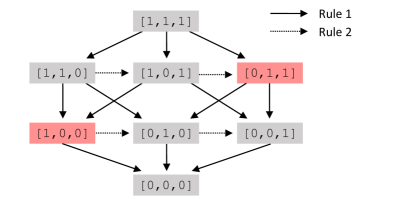
Figure 1: Hasse diagram illustrating the innate non-inferiority relationships amongst SERPs of length $k=3$.

Exhaustive Enumeration

Figure 1 summarizes all pairwise relationships amongst the $2^{k}=8$ SERPs of length $k=3$. Each arrow indicates a $\succeq$ relationship between the two indicated SERPs; and arrows are omitted in cases where they can be inferred via transitivity, with directed paths having the usual interpretation. There is no directed path between the two highlighted elements [1,0,0] and [0,1,1] and hence no non-inferiority relationship that connects them. As was noted earlier, that SERP pair is non-separable.

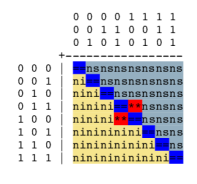
Figure 2: All SERP pairs of length $k=3$, and the relationships between them. Red cells indicate non-separability.

Figure 2 shows the same universe of eight $k=3$ SERPs using a different presentation. In each cell the SERP common to that row (with SERP bits read left-to-right, and $r_{1}$ first) is compared to the SERP common to the corresponding column (with SERP bits top-to-bottom, and $r_{1}$ at the top). The cells are color-coded: dark blue for SERPs that are equal (denoted ==); yellow for non-inferior relationships ($\succeq$, denoted ni); light blue for non-superior ($\preceq$, denoted ns); and red for non-separable (marked in the figure using **). This grid thus captures all $64$ relationships possible in Figure 1, and makes clear that there is only a single pair of $k=3$ SERPs that are non-separable, the pair highlighted in Figure 1.

Freedom!

We reiterate that while the score relativities shown in Figure 2 are innate and that there is thus little scope for divergence from the defined pairwise orderings, there are, nevertheless, many possible effectiveness metrics, even when $k=3$. That is because there is an infinity of score values that can be assigned that are compliant with the required pairwise SERP ordering constraints. For example, ${{\sf{Prec}}}@3$ assigns a different effectiveness score to each row of SERPs in Figure 1, has four different values possible ($0$, $1/3$, $2/3$, and $1$), and gives [1,0,1] and [0,1,1] the same score; whereas ${\sf{RR}}$@$3$ also assigns four values across the eight SERPs, but they are different ones ($0$, $1/3$, $1/2$, and $1$), and ${\sf{RR}}$@$3$ gives those same two SERPs different scores. Similarly, ${\sf{RBP}}(0.5)@3$ (rank-biased precision, see Moffat and Zobel, (2008) for a description) maps $k=3$ SERPs to a total of eight different scores, with each of the $2^{k}$ possible SERPs receiving a different metric score. Nevertheless, two SERPs related by $\succeq$ must have metric scores that numerically also comply; and they must comply in every plausible metric.

Table 1: The three possible effectiveness metric score relationships for the single non-separable SERP pair that arises when $k=3$.

Ordering	Metrics $M(\cdot)$ with that ordering
$M({\mbox{\tt{[1,0,0]}}})<M({\mbox{\tt{[0,1,1]}}})$	${{\sf{Prec}}}@3$, ${\sf{RBP}}(0.8)@3$, ${{\sf{AP}}}@3$, ${{\sf{NDCG}}}@3$
$M({\mbox{\tt{[1,0,0]}}})=M({\mbox{\tt{[0,1,1]}}})$	${{\sf{Succ}}}@3$, ${{\sf{RBP}}}((\sqrt{5}-1)/2)@3$
$M({\mbox{\tt{[1,0,0]}}})>M({\mbox{\tt{[0,1,1]}}})$	${{\sf{RR}}}@3$, ${{\sf{RBP}}}(0.5)@3$

It is only for non-separable pairs that the metric has ordering freedom. Table 1 provides examples of the three ordering relationships possible when considering the single $k=3$ non-separable pair shown in Figures 1 and 2. The metric ${{\sf{Succ}}}@k$ is $1$ if there is a relevant document anywhere in the top $k$, and $0$ otherwise; AP is average precision (Buckley and Voorhees,, 2005); and NDCG is normalized discounted cumulative gain (Järvelin and Kekäläinen,, 2002). Note that in the case of parameterized metrics like ${\sf{RBP}}$ the number of different scores produced and the numeric orderings attached to non-separable pairs can be affected by the metric parameter. In particular, the use of the golden ratio $\phi=(\sqrt{5}-1)/2\approx 0.62$ in the middle row of Table 1 gives equality for the non-separable SERP pair and thus allows ${\sf{RBP}}$ to yield all three possible arrangements of the two SERPs making up that non-separable pair.

Other Score Orderings

The choice of row and column ordering in Figure 2 is arbitrary (after all, SERPs are categorical data), and the visualization remains valid if the rows are permuted, or the columns are permuted, or both. There will always be eight blue cells, two red cells, and so on. That is, while Figure 2 employs a row and column ordering based upon lexicographic SERP representations as multi-dimensional vectors, other orderings could also be applied. As it turns out, a lexicographic ordering corresponds to the SERP score ordering induced by ${\sf{RBP}}(0.5)$. That is, Figure 2 can also be viewed as indicating the locations in the RBP$(0.5)$ score spectrum at which the non-separabilities arise when RBP$(0.5)$ is compared against other metrics. The blue cells form a perfect diagonal because the row and column orderings are identical.

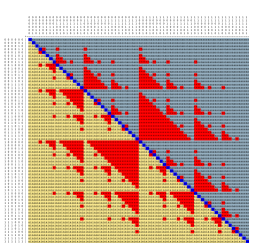
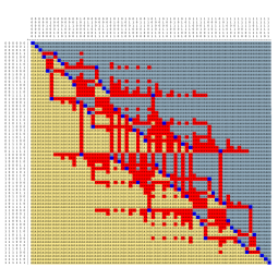
(a) RBP$(0.5)$ (lexicographic) on both	(b) RBP$(0.5)$ on left, NDCG on top
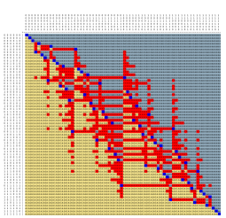
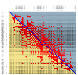
(c) AP on left, RBP$(0.5)$ on top	(d) AP on left, NDCG on top

Figure 3: All SERP pairs of length $k=6$, plotted using the same colors as in Figure 2, with each grid consisting of $2^{6}\times 2^{6}=4{,}096$ cells. Each pane has exactly the same number of red cells; they indicate SERP pairs where the two metrics are permitted to disagree on the relative ordering of the two SERPs, and are not in any way an indication that they do disagree.

Figure 3 shows what happens when SERPs of length $k=6$ are categorized in the same manner. Pane (a) directly corresponds to Figure 2, and orders the SERPs on both axes lexicographically, that is, by their RBP$(0.5)$ scores. Within pane (a) Figure 2 repeats eight times down the diagonal; the corresponding $k=4$ pattern appears four times; and the $k=5$ pattern arises twice. There are several other symmetries and motifs that recur in a fractal manner.

In Figure 3(b), the rows are still ordered by RBP$(0.5)$, but the columns are permuted into increasing NDCG score order (Järvelin and Kekäläinen,, 2002). Exactly the same number of each color cell is present, but they are now in a different arrangement. In pane (c) the rows are ordered by AP (Buckley and Voorhees,, 2005) and the columns are ordered by RBP$(0.5)$, yielding a third presentation of the same underlying data; and then pane (d) completes the set, with the rows ordered by AP and the columns ordered by NDCG. Across the four panes the three sets of $64$ blue cells have Kendall’s correlations, in the context of the four corresponding axis orderings, of $\tau=1.000$, $\tau=0.796$, $\tau=0.786$, and $\tau=0.976$ respectively. Not unexpectedly, AP is more closely correlated with NDCG than is RBP$(0.5)$, even when $k$ is just six.

Computing SERP Pair Categorizations

$\mbox{\emph{cumul}}\leftarrow 0$

2:$\mbox{\emph{been\_neg}}\leftarrow\mbox{\emph{been\_pos}}\leftarrow{\mbox{\bf{false}}}$

for $i\leftarrow 1$ to $k$ do

4:     $\mbox{\emph{cumul}}\leftarrow\mbox{\emph{cumul}}+{\mbox{\tt{S1}}}[i]$

     $\mbox{\emph{cumul}}\leftarrow\mbox{\emph{cumul}}-{\mbox{\tt{S2}}}[i]$

6:     if $\mbox{\emph{cumul}}<0$ then

         $\mbox{\emph{been\_neg}}\leftarrow{\mbox{\bf{true}}}$      

8:     if $\mbox{\emph{cumul}}>0$ then

         $\mbox{\emph{been\_pos}}\leftarrow{\mbox{\bf{true}}}$      

10:if been_neg and been_pos then

     return non-separable

12:else if been_pos then

     return non-inferior

14:else if been_neg then

     return non-superior

16:else

     return equal

Algorithm 1 Comparing SERPs to establish their innate ordering relationship. Each of S1 and S2 is a $k$-vector of 0s and 1s.

Algorithm 1 describes the comparison process used to compare pairs of SERPs and thus allow the creation of Figures 2 and 3. A linear scan tracking the cumulative sum of their element-by-element differences is sufficient to infer the relationship between any pair of $k$-SERPs S1 and S2. In particular, if there is no depth prior to $k$ at which S1 has fewer one-bits than has S2, then S1 must be either equal to S2, or non-inferior to it. On the other hand, if S1 has had both strictly fewer one-bits than S2 at some point $k^{\prime}\leq k$, and also strictly more one-bits than S2 at some other point $k^{\prime\prime}\leq k$, then S1 and S2 are non-separable.

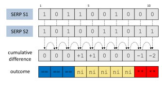
Figure 4: Comparing SERPs to get an innate pairwise ordering. In this example, either S1 or S2 might be assigned the higher score for metrics computed to depth $k=10$, possible because the two SERPs are non-separable. But at depths $k=4$ through to $k=8$ SERP S1 cannot be assigned a lower effectiveness score than SERP S2.

Figure 4 illustrates the application of Algorithm 1. At depths $i=1$, $i=2$, and $i=3$ the number of one-bits remains balanced and they appear in the same positions, and so the two SERPs are judged to be equal. From depth $i=4$ the cumulative difference is positive, and so the outcome switches to “non-inferior”. Finally, at $i=9$ the cumulative sum enters negative territory, and from that point onward the two SERPs must be regarded as being non-separable. Hence, any particular metric is free to assign any of the three possible relative orderings (Table 1) to these two $10$-SERPs. On the other hand, if only the first $k=5$ elements of S1 and S2 are considered, then every metric must assign a score to S1 that is not lower than the score assigned to S2. This variation with $i$ is typical: at first, any pair of SERPs are equal (when $i=0$); and then, after some number of relevance values have been considered, one of them gains the upper hand. That advantage either remains until the target depth $k$ is reached, or until the other SERP in turn claims the majority of one bits. If the latter occurs at any point the non-separability outcome cannot be subsequently reversed, and continues to hold as $i$ is further increased. No combination of further bits added in Figure 4 – positions $11$ to $20$, for example – could alter the outcome that results once $k=9$ is reached. Of course, each metric assigns a score to each of S1 and S2 for each value of $k$, and so for any given metric there is a score relativity. Once $k\geq 9$ that relativity can be in either direction.

We can now answer RQ1 in the affirmative: there are indeed sometimes fundamental relationships between SERPs that dictate the ordering of “@$k$” effectiveness scores, independently of the actual effectiveness metric used, and irrespective of the effectiveness scores assigned by that metric. We next explore implications of that in the context of typical IR batch evaluation scenarios, leading to a new way of presenting IR effectiveness results.

3 A New Perspective – IPSO

We are now in a position to consider RQ2, RQ3, and RQ4. First a test environment is described, and then using that data we explore the implications of these innate pairwise SERP orderings. For brevity – and because we think it is a fitting acronym – we reduce “innate pairwise SERP ordering” to IPSO. We then present our proposal for a new way of presenting IR system-vs-system experimental results, using IPSO as an additional indicator.

Experimental Setup

We make use of the runs submitted to the 2004 TREC Robust track Voorhees, (2004). A total of $110$ systems were represented via runs, with each system responding to a total of $249$ queries on documents from TREC Disks 4 and 5, excluding the Congressional Record from Disk 4. The official evaluation metric was AP, with ${{\sf{Prec}}}@10$ also reported. The Robust relevance judgments contain an average of $1250.6$ judgments per topic, of which $69.9$ had relevance grades of $1$ or greater. Our experiments assume binary judgments, with any documents judged $\geq 1$ taken to be relevant, and all unjudged documents assumed to be non-relevant.

Exhaustive Enumeration

RQ2 asks how frequently SERP pairs can be expected to display the innate ordering characteristics captured by the $\succeq$ relationship. We explore that in two ways – first via exhaustive enumeration of SERP pairs, and then by considering the SERP pairs that arise in a typical IR experimental setting.

Table 2: Fraction of SERP pairs of length $k$ that are equal, separable, and non-separable, based on enumeration ($k\leq 15$) and random generation of a billion SERP pairs ($k\geq 20$).

$k$	equal	separable	non-sep.
5	3.12%	83.98%	12.89%
10	0.10%	67.08%	32.81%
15	0.00%	55.97%	44.02%
20	0.00%	48.91%	51.09%
50	0.00%	31.43%	68.57%
100	0.00%	22.34%	77.66%

Table 2 categorizes the SERP pairs as $k$ increases, combining non-inferior and non-superior into a single separable grouping, as was described above. To form the table the values for $k\leq 15$ were computed exactly, via exhaustive counting over all possible $2^{2k}$ SERP-pair combinations using binary (0 or 1) relevance judgments. The three values for $k\geq 20$ are estimates, based on assessment of $10^{9}$ randomly-generated SERP pairs of each length, where random means that 0s and 1s are equally likely at each rank from $1$ through to $k$ in each of the SERPs.

The table indicates that a useful fraction of all possible SERP pairs can be innately ordered for moderate evaluation depths. For example, when $k=10$, fully two-thirds of all SERP pairs have a fixed relationship, and only one-third of SERP pair relativities are at the discretion of the individual metric. At $k=20$ that fraction is still around half; and even at $k=50$ around one third of all SERP-pair relativities can still be regarded as being metric-independent, and determined by application of the Rule 1 and Rule 2 that were introduced earlier.

Separability In Practice

Table 3: Fraction of SERP pairs of length $k$ that are equal, separable, and non-separable, based on all SERP-vs-SERP comparisons in the TREC Robust Track data across $249$ topics and $5{,}995$ system pairs.

$k$	equal	separable	non-sep.
5	20.40%	74.49%	5.12%
10	8.33%	74.66%	17.01%
15	4.91%	69.91%	25.18%
20	3.55%	66.01%	30.44%
50	1.54%	55.88%	42.58%
100	0.92%	50.44%	48.64%

Table 3 shows what happens when actual SERPs are considered. To build the table, all $110$ systems submitted to the Robust track were compared to each other, over all $249$ of the track topics, with all runs truncated at $100$ documents each. The results aggregate the $249\times 110\times 109/2=1{,}492{,}755$ resulting SERP-vs-SERP relationships. Compared to Table 2, a greater fraction of SERP pairs are identical, and a greater fraction of the SERP pairs are separable. The lower-than-expected non-separability levels suggest that these actual SERPs are not equivalent to being random. Non-randomness arises in two quite different ways. At low values of $k$ the proportion of 1s and 0s is approximately equal (for example, at $k=5$ there are $50.5$% non-relevant and $49.5$% relevant on average across the runs), but the placement of those outcomes within the SERPs tends to be correlated, as evidenced by the high number of “equal” outcomes in the first row in Table 3. The second effect is that as $k$ becomes larger there are far more non-relevant documents than relevant (for example, when $k=50$ the mix is $74.4$% 0s and $25.6$% 1s), caused in part by the systems seeking to bring relevant documents to the beginning of their runs, and then amplified by our application of the standard IR assumption that unjudged documents are not relevant.

To quantify the extent to which unjudged documents might be a confound, we explored the relevance judgments. Across the set of $110\times 259=27{,}390$ system-query runs, $18{,}817$ ($68.7$%) contained one or more unjudged documents, with the average position of the first unjudged document across those $18{,}817$ runs being rank $46.0$. Within that set of $18{,}817$ runs there were on average $14.6$ unjudged documents per $100$-item run. These numbers suggest that any measurements on the Robust runs that are taken at $k=100$ should be viewed with care, but that $k\leq 20$ measurements can be considered to be reasonably reliable. The appropriateness of using incomplete relevance judgments has been an ongoing theme of IR research for more than two decades, and we note that issue here without seeking to resolve it.

Regardless of the reasons, the fact that there are relatively high separability levels in common system-vs-system experimental settings at typical evaluation depths is an important outcome, and answers RQ2: a substantial fraction of paired SERP comparisons can indeed be ordered using nothing other than their innate relationship in the partial order that governs all SERPs. Furthermore, these SERP pairs have been confirmed to occur in practice Jones et al., (2015).

System Comparisons Over a Set of Topics

The fact that a high fraction of the SERP-vs-SERP pairs that arise in practice have innate orderings evident at plausible evaluation depths $k$ is very encouraging, and leads us to consider what happens across sets of topics.

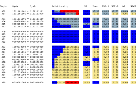
Figure 5: Comparison to depth $k=10$ between two Robust runs over Topics $301$–$325$. In the final six columns dark blue entries indicate equality of metric scores; yellow entries indicate that System $A$ scores more highly; and light blue values indicate that System $B$ scores more highly. The values in those cells are the score differences, $M(A)-M(B)$.

Figure 5 illustrates such a situation, taking a set of $25$ topics ($301$–$325$) and two of the Robust runs to depth $k=10$, denoted System $A$ and System $B$. Each row shows a topic number; the two SERPs being compared, one from System $A$ and one from System $B$; their IPSO relationship using the same labels and colors as were used in Figures 2 and 4; and then the metric score differences between System $A$ and System $B$ for that topic for each of six different effectiveness metrics. (Note that the metric scores are not shown, only their signed difference.)

At the same time the rows (topics) are ordered vertically into five sections: the first group contains all the non-separable topics ** that include an ns midpoint; the second group is all of the separable topics that lead to an ns outcome; the third group consists of all of the == topics; the fourth group shows the separable topics that lead to an ni outcome; and then the last group shows the single ** topic that has an ni midpoint. Within each of the five groups the rows are ordered by the number of red ** cells (if any), and then by the extent of the leading blue == zone. Given this overall ordering the rows can be thought of as “wrapping around” so that the bottom row is also adjacent to the top; making a cylinder that in fact contains four distinct sections rather than five.

Looking at the metric score differences shown in the final six columns of the figure, the “$\leq$” requirement when System $A$ and System $B$ are compared is clear in the second group of topics (starting at Topic $301$); and similarly the “$\geq$” requirement is clear in the fourth group of topics (starting at Topic $303$). On the other hand, the top group and bottom group have no such requirement, and in the top group (starting at Topic $302$) all three score difference possibilities can be seen, as was also noted in connection with Table 1. The one row that comprises the bottom group is consistent across the six illustrated metrics, but that is just chance, and light-blue ns overall outcomes could arise if further metrics were added.

 

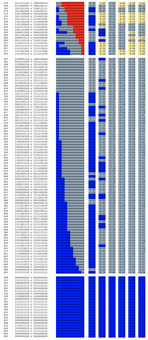
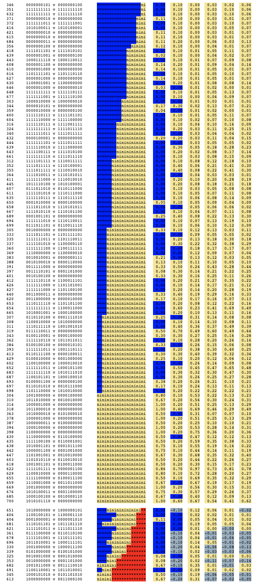
Figure 6: The IPSO comparison over all $249$ Robust topics to depth $k=10$ between the same two systems shown in Figure 5, using the same formatting and same column headings, but here split into two pieces that are presented side-by-side. The five sections of the output contain $20$ topics, $81$ topics, $23$ topics, $109$ topics, and $16$ topics respectively.

Figure 6 shows the same two Robust systems, but now with all $249$ topics included. There are again five distinct groups, or four when the top row is considered to be “adjacent” to the bottom row, wrapped around a cylinder. Moreover, with $81$ topics in the second group, $23$ topics in the middle group, and $109$ topics in the fourth group, it is clear that for the great majority of topics the IPSO analysis is sufficient to identify the polarity of the paired SERP score differences. Those mandated relationships are clearly visible for the six metrics at the right of Figure 6, with columns for ${\sf{RR}}$, ${{\sf{Prec}}}@10$, ${\sf{RBP}}(0.5)$, ${\sf{RBP}}(0.8)$, ${\sf{AP}}$, and ${\sf{NDCG}}$, as in Figure 5. Only $36$ of the topics yield $k=10$ SERP pairs for which an effectiveness metric is free to assign scores in either order. In those two sections of Figure 6 both positive (yellow) and negative (light blue) metric score differences do arise. But in the long second and fourth sections there is an enforced inequality relationship on the per-topic score differences that simply cannot be violated.

Statistical Testing

The penultimate step in most system-vs-system experimental comparisons is to carry out a paired statistical test on the metric score differences, to establish the degree of support for the null hypothesis that the mean difference is zero. (The ultimate step being, of course, to crystallize the findings in to a research paper submission). If there is only limited support for the null hypothesis (with “limited” often at a level of $p<0.05$) it is rejected, and the difference between the two systems is deemed to be “significant”.

The IR community is well-versed in these techniques, and now expects statistical testing, in one way or another, as a matter of routine (Sakai, 2016a, ; Sakai, 2016b, ; Urbano et al.,, 2019; Smucker et al.,, 2007; Ferro and Sanderson,, 2022). The Student $t$ test is probably the most commonly used option, but the Wilcoxon Signed-Rank test and the simpler Sign test can also be used, especially if the distribution of paired score differences does not match the requirements for the parametric Student test (such as when the metric being used is RR).

Application of the IPSO mechanism generates a set of five category counts, but not scores. Nor are there any score differences. That means it is not possible to compute a $p$ value from the Student $t$ test or from the Wilcoxon Signed-Rank test. However, it is possible to employ a Sign test, because it applies to categories rather than to values. As an example, consider the system-vs-system relationship depicted in Figure 6. If the first and last groups of topics (of the five groups) are discarded as being inconclusive, and the middle group is discarded as being uninformative, what remains is a set of $81$ ns topics and a set of $109$ ni topics. It is then possible to pose as a null hypothesis that “the number of ns topics is equal to the number of ni topics”, and compute a $p$ value relative to that hypothesis using the Sign text. For the two illustrated runs that results in $p=0.0499$ as a two-tailed outcome, and we can conclude that the difference between $|{\mbox{\tt{ns}}}|=81$ and $|{\mbox{\tt{ni}}}|=109$ is significant at the $0.05$ level. Note that it is the counts of the ni and ns topic sets that contribute to the test, without reference to the overall topic set size. That way, if the ni and ns sets are closer to each other in size, or if the two non-separable groups span the majority of the topics and the ni and ns sets are small, the power available to the Sign test will also be small, and the calculated $p$ values will tend to be larger.

The $p$ values computed in this manner must not be extrapolated as applying to the overall system comparison for other metrics; to do so would be incorrect. This is because in a normal score-based statistical test across a full set of topics the queries are taken to be independent draws from the population of all possible queries. A small $p$ value then supports predictions that further independent draws from the same underlying population will demonstrate the same relationship between the two systems. But in the scenario considered here the set of ** topics across which any such extrapolation would need to apply cannot be regarded as being independent draws, and there is a selection bias. Indeed, they are quite explicitly known to not have the same characteristics as the ones that led to the ns and ni sets. Moreover, as a further complexity, note that those two key classes, ns and ni, are “not superior” and “not inferior”, with both including the possibility of metric score equality. That is, a system comparison could, conceivably, assign every single topic to the ns set (or, equally, the ni set) and thereby attain a miniscule IPSO-based Sign test $p$ value, and yet for a particular metric, still have System $A$ and System $B$ assigned identical scores for every one of those topics.

Taking again the specific example shown in Figure 6, there are $|{\mbox{\tt{**}}}|=36$ queries for which each effectiveness metric is free to assign numeric scores in either relative order, and any IPSO-based claims that are made must of necessity respect that freedom. Hence, depending on the metric, the final balance of “votes” between System $A$ and System $B$ might be anywhere between $81$ “versus” $109+36$ (which yields $p<0.01$) at one extreme, and $81+36$ versus $109$ (which results in $p\approx 0.25$) at the other.

That is, the Sign test $p$ value generated from an IPSO-based analysis and the null hypothesis $|{\mbox{\tt{ns}}}|=|{\mbox{\tt{ni}}}|$ may be regarded as being an interesting indicator of overall system relativities, but must not be taken as a measurement of statistical confidence that makes promises in regard to all metrics.

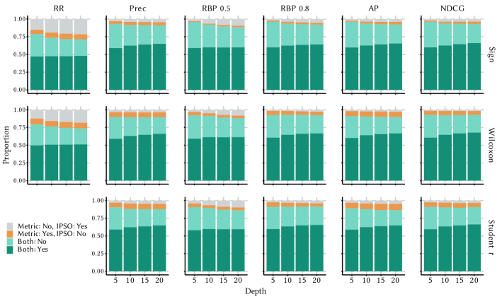
Figure 7: Statistical test outcomes for all $110\times 109/2=5{,}995$ System $A$ versus System $B$ challenger-vs-champion experiments possible within the $110$ submitted Robust runs. In each case all $249$ topics are used, with six effectiveness metrics then employed at each of four different retrieval depths; three statistical tests (two-tailed in each case); and a significance threshold of $p<0.05$. The two-tailed Sign test is always used to obtain the IPSO $p$ values, and they refer to the null hypothesis $|{\mbox{\tt{ns}}}|=|{\mbox{\tt{ni}}}|$.

Given this context, Figure 7 explores the relationship between IPSO-derived Sign test $p$ values (for the null hypothesis $|{\mbox{\tt{ns}}}|=|{\mbox{\tt{ni}}}|$) and those generated via a range of metrics (for the null hypothesis that the two systems have the same performance as assessed by that metric) in conjunction with three different statistical tests. Each bar in each pane of the figure takes all possible System $A$ versus System $B$ pairs in the Robust data, and applies one effectiveness metric to one depth $k$, and then applies one selected statistical test to the set of paired score differences, to compute a $p$ value. Each of those $(A,B)$ system pairs in each bar of each subgraph is then labeled as being one of four possible categories:

• “Both: Yes”, indicating that the IPSO Sign test (comparing $|{\mbox{\tt{ns}}}|$ and $|{\mbox{\tt{ni}}}|$) and the selected metric/test pair (comparing System $A$ and System $B$) agree that there is a significant difference;

• “Both: No”, when the IPSO Sign test and the selected metric/test pair agree that there is not a significant difference;

• “Metric: Yes”, where the metric/test combination reports significance, but IPSO does not; and, finally

• “Metric: No”, where IPSO reports significance, but the metric/test combination between System $A$ and System $B$ does not.

Of these four possibilities, the combined “Both: Yes” and “Both: No” categories represent a reassuringly high level of agreement. They are shown in Figure 7 as two shades of green at the bottom of each of the bars in each of the panes, and cover a minimum (across the bars and panes) of three quarters of all system pairs, and up to $90$% or more of the system pairs in some metric/test cases. Note also how (with the exception of ${\sf{RR}}$) the fraction of “Both: Yes” tends to increase with $k$ regardless of metric and statistical test; and how for any given metric the increased power of the Wilcoxon and then $t$ tests relative to the Sign test is visible via the growth of the mustard-colored “Metric: Yes” category when moving down each column of graphs.

The non-green minority of cases represent system pairs for which disagreement occurs. Figure 8 helps understand the situations in which that happens. To form each pane the $110$ systems submitted to the Robust track were ordered by average ${{\sf{Prec}}}@10$ score, and then the $5{,}995$ individual system-vs-system experiments that were aggregated into the “${{\sf{Prec}}}@10$, $k=10$, Student $t$ test” bar in Figure 7 were each represented by a colored dot placed according to the ranks of the two systems. For example, the dot at bottom left in each pane represents the “best” versus “second best” system, and the dot at top right is “second worst” versus “worst”. Dots along the diagonal edge similarly represent systems being compared to the ones immediately adjacent to them in the system ordering induced by ${{\sf{Prec}}}@10$.

In each of the four panes in Figure 8 there is a distinctive pattern of dark green (both ${{\sf{Prec}}}@10$ and ${\sf{IPSO}}$ indicate significance) and light green (neither indicate significance), with a transition region between of grey and mustard-colored points. Note how increasing the stringency of the significance threshold (moving from pane (a) to pane (b), and similarly moving from pane (c) to pane (d)) and reducing the number of topics employed (moving from pane (a) to pane (c), and similarly moving from pane (b) to pane (d)) both shift the balance between dark green and light green, but don’t alter the overall pattern. Note also how the grey “${\sf{IPSO}}$ only” cells tend to spread into (that is, be surrounded by) the light green zone, whereas the mustard-colored “${{\sf{Prec}}}@10$ only” cells tend to spread into the dark green zone. In Figure 8(a), $67.4$% of the plotted dots are dark green and $7.5$% are mustard, with ${{\sf{Prec}}}@10$ identifying a total of $74.9$% of system pairs as being significantly different when the Student $t$ test is employed. On the other hand, ${\sf{IPSO}}$ and the Sign test achieve a total of $71.4$%. That these rates are different is of no concern. In particular, the statistical tests are different, and ${\sf{IPSO}}$ significance is in one sense a broader outcome than is ${{\sf{Prec}}}@10$ significance, making it harder to achieve, but at the same time is also a weaker outcome, since it is based only on the ns and ni counts (with both groups permitting score equality), rather than on score differences.

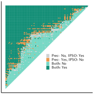
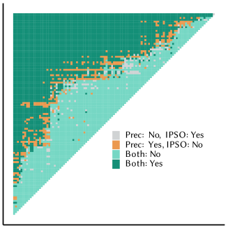
(a) $249$ topics, $p<0.05$	(b) $249$ topics, $p<0.01$
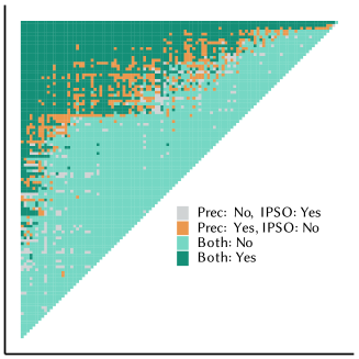
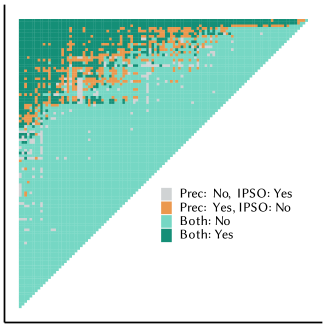
(c) $50$ topics, $p<0.05$	(d) $50$ topics, $p<0.01$

Figure 8: System-vs-system significance categories, with one “dot” plotted per system pair using colors that match Figure 7. The ordering of the $110$ Robust systems is based on their average ${{\sf{Prec}}}@10$ score across the given topic set (all $249$ topics in the top two panes, and topics $301$–$350$ in the bottom two panes), and with system-vs-system significance calculated from paired ${{\sf{Prec}}}@10$ scores using the Student $t$ test.

The two systems depicted in Figures 5 and 6 are in fact the best Robust run and the $25$ th percentile run according to ${{\sf{Prec}}}@10$ – which, as a pair, correspond to points 1/4 of the way up the triangle’s left edge in each pane of Figure 8. Direct metric-based comparisons of these two runs can also be carried out, of course. For example, ${{\sf{Prec}}}@10$ yields $p=0.017$ using a two-tailed Student $t$ test, and ${\sf{NDCG}}$ gives $p=0.027$. On the other hand, ${\sf{AP}}$, ${\sf{RBP}}(0.5)$, and ${\sf{RBP}}(0.8)$ all result in $p\geq 0.05$. This kind of variability is inevitable when statistical tests are employed to gauge significance, and the reassurance, or “hedge” as it was described above, is provided by noting that all six metrics assess the first run as being better than the second. Such differences in system performance can exist without a statistical test passing some selected – but also arbitrary – threshold. The critical point that we seek to make in this work is that the IPSO-based Sign test has the capacity to encompass all of those metric-specific outcomes and provide overall guidance as to the likely ordering of the two systems.

The results we have presented thus answer RQ3: IPSO-derived system-vs-system relationships generally agree with those of conventional effectiveness metrics under commonly applied statistical tests.

Using IPSO as a Corroboration

We have now arrived at our proposal. As was noted earlier, it is common for researchers reporting the result of a system-vs-system comparison to tabulate several metrics, and a statistical test for each, as a way of providing multiple sources of evidence that their new challenger system does indeed outperform the current champion. We propose instead that the hedging aspect of multi-metric analysis be supported by an IPSO-based system comparison.

For example, suppose that two systems $A$ (champion) and $B$ (challenger) are being compared in regard to their suitability for some defined search task. We suggest that the comparison be carried out as follows:

• Select a single evaluation metric $M(\cdot)$ for which the corresponding user model can be argued as matching the anticipated (or observed) behavior of searchers when carrying out that task, and the way that particular user population might therefore define and measure “search success”;

• Report mean metric scores $M(A)$ and ${M}(B)$ and the mean score difference $M(B)-M(A)$ (the measured effect size);

• Then carry out a suitable significance test against the null hypothesis that “the effect size is zero”;

• If that test yields a $p$ value less than some stipulated threshold $\alpha$ (typically $\alpha=0.05$), then “add a $\dagger$” and claim significance;

• Plus, if the metric-based $p$ value is less than $\alpha$, perform an IPSO-based Sign test against the null hypothesis that “the number of ns topics and the number of ni topics is the same”;

• And if $p<\alpha$ from that second test as well, add that further claim (by adding a $\ddagger$, or some other preferred symbol) to the reported results, as a corroboration of generality.

That is, we argue in response to RQ4 that one IPSO-based test “in the hand” is worth multiple other metrics “in the bush” when seeking to add generality to an evaluation that has, for principled reasons, been based on a chosen user-matched effectiveness metric.

Implications and Limitations

If a single pair of SERPs lead to an IPSO outcome of ni or ns, then the relationship between the two SERPs in an “at $k$” comparison is certain and is metric-agnostic. On the other hand, as has been noted above, if an IPSO-based Sign test over a set of topics yields a significant outcome, there is still no confidence that the outcome is applicable to all of the tested topics, nor to all future topics. That lack of confidence is partly a consequence of the nature of statistical testing – it gives encouragement (based on a representative sample) but never certainty; and is partly a consequence of the fact that IPSO is an imprecise indicator, with the ns and ni classes both admitting score equality, and with the ** class able to swing either way.

Also worth noting is that – as is also the case for standard metric scores – each SERP length $k$ is likely to lead to a different computed $p$ value. In the case of most metrics, as the evaluation depth increases, so too does the likelihood of significance, an effect that was identified in connection with Figure 7. But in the case of IPSO, the fact that the ni and ns topic counts in any given set cannot increase as $k$ increases means that the $p$ value will, other things being equal, also tend to increase. That is, the greater the value of $k$, the less likely will be a Sign test $p$ value that is below the threshold. We will undertake further experimentation to explore this aspect of our proposal.

Graded Relevance

The examples used as illustrations in the previous section all made use of binary relevance labels; as did the collections and runs used in the experiments presented in this section. But exactly the same definitions (Rule 1 and Rule 2) can be applied to real-valued (ratio scale) SERP comparisons, without any adjustments being required. Similarly, Algorithm 1 remains the correct description of the comparison computation, except that S1 and S2 are now vectors of floating point values. For example, if relevance is being reported on a four-point ratio scale, $r_{i}\in\{0.0,0.2,0.8,1.0\}$ say, and we have $k=5$, then ${\mbox{\tt{S1}}}=[1.0,0.8,0.0,0.2,1.0]$ and ${\mbox{\tt{S2}}}=[0.8,0.8,0.0,0.2,0.8]$ have the relationship ${\mbox{\tt{S1}}}\succeq{\mbox{\tt{S2}}}$ because of Rule 1; and if ${\mbox{\tt{S3}}}=[1.0,0.2,0.0,0.8,1.0]$ then ${\mbox{\tt{S1}}}\succeq{\mbox{\tt{S3}}}$ because of Rule 2; and S2 and S3 are non-separable.

If the relevance grades are ordinal classes such as “not at all”, “somewhat”, and “highly”, then a gain mapping that converts ordinal relevance grades to floating point values must be argued for and applied first, in exactly the way as is needed for all numeric score comparisons based on graded relevance evaluations. That is, Algorithm 1 may not be applied directly to relevance grades such as $r_{i}\in\{0,1,2\}$ representing $r_{i}\in\{\mbox{\emph{not at all}},\mbox{\emph{somewhat}},\mbox{\emph{highly}}\}$, because the computation in Algorithm 1 requires addition, and ordinal class labels such as “somewhat” may not be summed, even when it represented by the faux-integer value of “1”. That is, the ordinal-to-numeric gain mapping (Moffat,, 2022) must be specified before the scoring can be considered, and while IPSO provides metric-independent assessments, it cannot be gain-mapping-independent.

Experimental evaluations in graded-relevance measurement contexts will be carried out as future work.

4 Related Work

The most pertinent prior work is that of Diaz and Ferraro, (2022). Their recall paired preference (RPP) approach also carries out SERP comparisons “without effectiveness metrics”. In this mechanism a distribution over users is assumed as to how many relevant items are being sought from the SERPs, and for each user the SERP that delivers that many relevant documents more quickly is the one that is preferred. As a distinction to previous work, Diaz and Ferraro, note that, like AP, their probability distribution is over recall levels rather than rank positions, differentiating from metrics such as RBP and DCG. The relationship between two SERPs is then determined by forming a preference expectation over the defined user population. Like our IPSO method, RPP reports an ordering between two SERPs rather than scores for single SERPs that must then be compared. In the case of Diaz and Ferraro,, the distribution of user goals informs the outcome and a SERP pair always leads to a $<$, $=$, or $>$ outcome. In our work here we assume that users look at $k$ or fewer documents, seeking generality that covers all $@k$ metrics, once the validity of Rules 1 and 2 is accepted; but thus also needing to allow “don’t know” answers (the non-separable pairs) as well as $\leq$, $=$, and $\geq$ determinations. Diaz, (2023) and Diaz and Mitra, (2023) go on to consider two further formulations to inform our understanding of how to compare SERPs with each other: lexiprecision and lexirecall, developed by considering the lexicographic properties of SERPs. These methods compare SERPs based on the position in the ranking of the first relevant item that is not matched by relevance in the other SERP, or the rank position of the $p$ th relevant item for some selected value $p$, or the rank position of the last relevant item, or some amalgam of such values.

In earlier work that anticipates our proposal here, Jones et al., (2015) note that there is only a subset of depth-$k$ rankings on which metrics can disagree. They then provide exhaustive experimentation on ranked results lists of depth $k=10$, with a total of $10$ relevant documents available (resulting in $1{,}023$ such lists when ignoring the “all zeros” ranking), and confirm that all such rankings do occur in organic ranking tasks, by empirically examining submitted TREC runs. They also provide a more detailed analysis on when metrics tend to disagree, and explore properties that may be predictive of such disagreement.

The relationship between user behavior and the underlying quality of ranked results lists has been explored by a range of authors, resulting in a number of metrics for evaluating such rankings (Moffat and Zobel,, 2008; Robertson,, 2008; Chapelle et al.,, 2009; Robertson et al.,, 2010) and a greater understanding of the relationship these metrics have with assumed user models (Sakai and Robertson,, 2008; Chapelle et al.,, 2009; Dupret and Piwowarski,, 2010; Dupret,, 2011; Carterette,, 2011; Carterette et al.,, 2012; Moffat et al.,, 2017; Wicaksono and Moffat,, 2018; Zhang et al., 2020a, ; Moffat et al.,, 2022). The overarching theme of all of these papers is that metric scores should be formulated in the context of how users are likely to derive information from SERPs, so as to allow the computed scores to reflect an informative quantity; it is our strong desire to retain and embrace that connection that has informed our proposal here. In particular, it is important to note that we are not arguing for IPSO evaluation to supersede metric-based evaluation; rather, we suggest IPSO as an augment for a well-chosen metric.

Ideally, a metric score should be reflective of user satisfaction, as this is what ultimately matters when measuring ranked retrieval systems. To this end, a number of works have sought to establish a connection between metric score and user satisfaction. This then allows metrics to be, at least in part, validated against the user experience (Huffman and Hochster,, 2007; Jiang and Allan,, 2016; Mao et al.,, 2016; Chen et al.,, 2017; Su et al.,, 2018; Liu et al.,, 2018; O’Brien et al.,, 2020; Zhang et al., 2020b, ; Sakai and Zeng,, 2021; Moffat et al.,, 2022). On the other hand, Alex et al., (2022) have recently noted use cases in which it could be important to measure SERP differences that might not be discernible by users, such as in diagnostic situations, or perhaps as a model training objective.

Ferrante et al., (2017, 2021) have presented arguments to the effect that many traditional effectiveness metrics may not be well-founded from a measurement point of view because they are not on an interval scale; a claim that is strongly contested (Sakai,, 2020; Moffat,, 2022). Irrespective of the outcome of that debate, IPSO presents a metric-free way of carrying out system comparisons to obtain guidance as to which system might be preferable. Indeed, this is one inherent benefit of the Sign test, which does not require magnitudes of differences for meaningful hypothesis testing.

Moffat, (2013) categorizes metrics according to seven numeric properties, including some that embed Rules 1 and 2; and a number of other researchers have also considered measuring effectiveness from what is referred to as an “axiomatic” viewpoint, of which Rules 1 and 2 are instances (Bollmann,, 1984; Busin and Mizzaro,, 2013; Amigó et al.,, 2017; Gupta et al.,, 2019; Amigó et al.,, 2020; Giner,, 2022). Axiomatic approaches have also been used in the quest for retrieval models (Fang and Zhai,, 2005).

The process of planning and executing experimental system comparisons has also received considerable attention, including in regard to topic set size and statistical testing practices (Smucker et al.,, 2007; Sakai, 2016b, ; Sakai, 2016a, ; Urbano et al.,, 2019; Ferro and Sanderson,, 2022). Sakai, 2016b considers the design of batch retrieval experimentation in terms of the number of topics to employ to reach statistically valid outcomes. Sakai, 2016a also provides a detailed systematic review on testing practices across over $1000$ SIGIR and TOIS papers from 2006 to 2015. Other work has explored the reliability and predictivity of typical batch IR experiments and measurement protocols (Cormack and Lynam,, 2006; Rashidi et al.,, 2021) and some of the limitations therein (Zobel,, 2023).

Finally, work that describes the overall process of batch evaluation and issues that arise in the formation of relevance judgments may also be of interest to the reader (Saracevic,, 1995; Voorhees,, 2002; Buckley and Voorhees,, 2004, 2005; Sakai and Kando,, 2008; Sanderson,, 2010; Hofmann et al.,, 2016).

5 Conclusion

We have described IPSO, a mechanism for comparing two SERPs that is based on fundamental ordering criteria that apply to every plausible effectiveness metric. While IPSO is not itself a metric, and does not generate effectiveness scores, it can nevertheless be used as input to the Sign test and hence derive a $p$ value when two systems are being compared over a set of topics. That is, IPSO can be used to provide evidence that a measured relationship in a challenger-vs-champion experiment holds not just for the chosen metric – which for experimental fidelity reasons should always be selected (and/or parameterized) based on the user characteristics that are anticipated for that type of search – but (subject to the limitations we have noted) for other metrics as well. In particular, a System $A$ versus System $B$ comparison]using a chosen metric $M(\cdot)$ in which $M(A)-M(B)<0$ with statistical confidence that is accompanied by an IPSO-based significance outcome that also favors System $B$ is a stronger result than one based solely on the metric alone, and an augmented evaluation of the suggested type may be a more powerful demonstration of generality than is possible with a table employing multiple different effectiveness metrics.

The new IPSO mechanism also has limitations, of course. First is the need to understand that it is a comparison tool, not a metric than can be used to score runs. It does not provide a numeric value that tells you how good a SERP is in isolation, and even when it says that one SERP is “not inferior” to another, it cannot quantify the extent of the possible superiority. Nor can it indicate how close to being “perfect” any particular run is. For those tasks, a metric is required, meaning that a specific user model must also have been selected. As noted earlier, care is also required when interpreting the IPSO-derived $p$ values. Any significance observed relates to the null hypothesis $|{\mbox{\tt{ns}}}|=|{\mbox{\tt{ni}}}|$, and not to the more targeted hypothesis that “System $A$ and System $B$ have the same performance when measured using metric $M(\cdot)$”.

Nor is IPSO invariant in its evaluation with regard to depth $k$. As can be seen in Figure 4, any given IPSO evaluation is likely to start by indicating equality between the two SERPs (this is the starting point for $k=0$, of course), then shift to a period of either “non-inferior” or “non-superior”, and then, as $k$ gets even larger (and sufficiently deep judgment are available to support continued evaluation), may well undertake a second transition to “non-separable”. That is, an IPSO Sign-test relationship established at one value of $k$ might not continue to apply at a larger value of $k$. We note that the same risk also applies to comparisons based on metric scores – a significant relationship established at one value for $k$ might not be recognized as being significant at a different value of $k$. As a component of further experiments to investigate more closely any sensitivity to the value of $k$, we also need to carry out an extended experimental comparison across a range additional datasets, including ones that employ graded-relevance scoring regimes, in order to provide further assurance that IPSO leads to outcomes that can be usefully interpreted.

Despite these limitations, we recommend that researchers incorporate IPSO into their experimental tool chains, and employ our suggested reporting framework in which one metric is adopted, defended, and then deployed, with IPSO used as the “hedge” to provide evidence in regard to generality.

Finally, note that the definition of IPSO is fundamentally tied to the assumption that users consume each SERP sequentially. We posit that to be a reasonable assumption for traditional linear text/link-based SERPs (and note that many previous authors have also employed the same assumption), but it may not apply to (for example) the two-dimensional SERP presentations that emerge from image and product search. Each user of those services may have a regular browsing sequence that they tend to follow, but different users might have different inspection orderings. Extending our analysis to this important case in a key area for future work.

Software

Source code to allow IPSO-based comparisons on pairs of SERPs is provided at https://github.com/JMMackenzie/IPSO.

Acknowledgements

This work was in part supported by the Australian Research Council (project DP190101113). We thank the referees for their supportive and insightful comments.

References

- Alex et al., (2022) Alex, J., Hall, K., and Metzler, D. (2022). Atomized search length: Beyond user models. arXiv:2201.01745.
- Amigó et al., (2017) Amigó, E., Fang, H., Mizzaro, S., and Zhai, C. (2017). Axiomatic thinking for information retrieval: And related tasks. In Proc. ACM Int. Conf. on Research and Development in Information Retrieval (SIGIR), pages 1419–1420.
- Amigó et al., (2020) Amigó, E., Fang, H., Mizzaro, S., and Zhai, C. (2020). Axiomatic thinking for information retrieval: Introduction to special issue. Information Retrieval, 23:187–190.
- Bollmann, (1984) Bollmann, P. (1984). Two axioms for evaluation measures in information retrieval. In Proc. ACM Int. Conf. on Research and Development in Information Retrieval (SIGIR), pages 233–245.
- Buckley and Voorhees, (2004) Buckley, C. and Voorhees, E. M. (2004). Retrieval evaluation with incomplete information. In Proc. ACM Int. Conf. on Research and Development in Information Retrieval (SIGIR), pages 25–32.
- Buckley and Voorhees, (2005) Buckley, C. and Voorhees, E. M. (2005). Retrieval system evaluation. In Voorhees, E. M. and Harman, D. K., editors, TREC: Experiment and Evaluation in Information Retrieval, chapter 3, pages 53–78. MIT Press.
- Busin and Mizzaro, (2013) Busin, L. and Mizzaro, S. (2013). Axiometrics: An axiomatic approach to information retrieval effectiveness metrics. In Proc. Int. Conf. on Theory of Information Retrieval (ICTIR), pages 22–29.
- Carterette, (2011) Carterette, B. (2011). System effectiveness, user models, and user utility: A conceptual framework for investigation. In Proc. ACM Int. Conf. on Research and Development in Information Retrieval (SIGIR), pages 903–912.
- Carterette et al., (2012) Carterette, B., Kanoulas, E., and Yilmaz, E. (2012). Incorporating variability in user behavior into systems based evaluation. In Proc. ACM Int. Conf. on Information and Knowledge Management (CIKM), pages 135–144.
- Chapelle et al., (2009) Chapelle, O., Metzler, D., Zhang, Y., and Grinspan, P. (2009). Expected reciprocal rank for graded relevance. In Proc. ACM Int. Conf. on Information and Knowledge Management (CIKM), pages 621–630.
- Chen et al., (2017) Chen, Y., Zhou, K., Liu, Y., Zhang, M., and Ma, S. (2017). Meta-evaluation of online and offline web search evaluation metrics. In Proc. ACM Int. Conf. on Research and Development in Information Retrieval (SIGIR), pages 15–24.
- Cormack and Lynam, (2006) Cormack, G. V. and Lynam, T. R. (2006). Statistical precision of information retrieval evaluation. In Proc. ACM Int. Conf. on Research and Development in Information Retrieval (SIGIR), pages 533–540.
- Diaz, (2023) Diaz, F. (2023). Best-case retrieval evaluation: Improving the sensitivity of reciprocal rank with lexicographic precision. arXiv:2306.07908v1.
- Diaz and Ferraro, (2022) Diaz, F. and Ferraro, A. (2022). Offline retrieval evaluation without evaluation metrics. In Proc. ACM Int. Conf. on Research and Development in Information Retrieval (SIGIR), pages 599–609.
- Diaz and Mitra, (2023) Diaz, F. and Mitra, B. (2023). Recall, robustness, and lexicographic evaluation. arXiv:2302.11370v4.
- Dupret, (2011) Dupret, G. (2011). Discounted cumulative gain and user decision models. In Proc. Symp. on String Processing and Information Retrieval (SPIRE), pages 2–13.
- Dupret and Piwowarski, (2010) Dupret, G. and Piwowarski, B. (2010). A user behavior model for average precision and its generalization to graded judgments. In Proc. ACM Int. Conf. on Research and Development in Information Retrieval (SIGIR), pages 531–538.
- Fang and Zhai, (2005) Fang, H. and Zhai, C. (2005). An exploration of axiomatic approaches to information retrieval. In Proc. ACM Int. Conf. on Research and Development in Information Retrieval (SIGIR), pages 480–487.
- Ferrante et al., (2021) Ferrante, M., Ferro, N., and Fuhr, N. (2021). Towards meaningful statements in IR evaluation: Mapping evaluation measures to interval scales. IEEE Access, 9:136182–136216.
- Ferrante et al., (2017) Ferrante, M., Ferro, N., and Pontarollo, S. (2017). Are IR evaluation measures on an interval scale? In Proc. Int. Conf. on Theory of Information Retrieval (ICTIR), pages 67–74.
- Ferro and Sanderson, (2022) Ferro, N. and Sanderson, M. (2022). How do you test a test? A multifaceted examination of significance tests. In Proc. Conf. on Web Search and Data Mining (WSDM), pages 280–288.
- Giner, (2022) Giner, F. (2022). On the effect of ranking axioms on IR evaluation metrics. In Proc. Int. Conf. on Theory of Information Retrieval (ICTIR), pages 13–23.
- Gupta et al., (2019) Gupta, S., Kutlu, M., Khetan, V., and Lease, M. (2019). Correlation, prediction and ranking of evaluation metrics in information retrieval. In Proc. European Conf. on Information Retrieval (ECIR), pages 636–651.
- Hofmann et al., (2016) Hofmann, K., Li, L., and Radlinski, F. (2016). Online evaluation for information retrieval. Foundations & Trends in Information Retrieval, 10(1):1–117.
- Huffman and Hochster, (2007) Huffman, S. B. and Hochster, M. (2007). How well does result relevance predict session satisfaction? In Proc. ACM Int. Conf. on Research and Development in Information Retrieval (SIGIR), pages 567–574.
- Järvelin and Kekäläinen, (2002) Järvelin, K. and Kekäläinen, J. (2002). Cumulated gain-based evaluation of IR techniques. ACM Trans. on Information Systems, 20(4):422–446.
- Jiang and Allan, (2016) Jiang, J. and Allan, J. (2016). Correlation between system and user metrics in a session. In Proc. ACM SIGIR Conf. on Human Information Interaction and Retrieval (CHIIR), pages 285–288.
- Jones et al., (2015) Jones, T., Thomas, P., Scholer, F., and Sanderson, M. (2015). Features of disagreement between retrieval effectiveness measures. In Proc. ACM Int. Conf. on Research and Development in Information Retrieval (SIGIR), pages 847–850.
- Liu et al., (2018) Liu, M., Liu, Y., Mao, J., Luo, C., Zhang, M., and Ma, S. (2018). “Satisfaction with failure” or “unsatisfied success”: Investigating the relationship between search success and user satisfaction. In Proc. Conf. on the World Wide Web (WWW), pages 1533–1542.
- Mao et al., (2016) Mao, J., Liu, Y., Zhou, K., Nie, J., Song, J., Zhang, M., Ma, S., Sun, J., and Luo, H. (2016). When does relevance mean usefulness and user satisfaction in web search? In Proc. ACM Int. Conf. on Research and Development in Information Retrieval (SIGIR), pages 463–472.
- Moffat, (2013) Moffat, A. (2013). Seven numeric properties of effectiveness metrics. In Proc. Asia Information Retrieval Societies Conf. (AIRS), pages 1–12.
- Moffat, (2022) Moffat, A. (2022). Batch evaluation metrics in information retrieval: Measures, scales, and meaning. IEEE Access, 10:105564–105577.
- Moffat et al., (2017) Moffat, A., Bailey, P., Scholer, F., and Thomas, P. (2017). Incorporating user expectations and behavior into the measurement of search effectiveness. ACM Trans. on Information Systems, 35(3):24.1–24.38.
- Moffat et al., (2022) Moffat, A., Mackenzie, J., Thomas, P., and Azzopardi, L. (2022). A flexible framework for offline effectiveness metrics. In Proc. ACM Int. Conf. on Research and Development in Information Retrieval (SIGIR), pages 578–587.
- Moffat and Zobel, (2008) Moffat, A. and Zobel, J. (2008). Rank-biased precision for measurement of retrieval effectiveness. ACM Trans. on Information Systems, 27(1):2.
- O’Brien et al., (2020) O’Brien, H. L., Arguello, J., and Capra, R. (2020). An empirical study of interest, task complexity, and search behaviour on user engagement. Information Processing & Management, 57(3):102226.
- Rashidi et al., (2021) Rashidi, L., Zobel, J., and Moffat, A. (2021). Evaluating the predictivity of IR experiments. In Proc. ACM Int. Conf. on Research and Development in Information Retrieval (SIGIR), pages 1667–1671.
- Robertson, (2008) Robertson, S. E. (2008). A new interpretation of average precision. In Proc. ACM Int. Conf. on Research and Development in Information Retrieval (SIGIR), pages 689–690.
- Robertson et al., (2010) Robertson, S. E., Kanoulas, E., and Yilmaz, E. (2010). Extending average precision to graded relevance judgments. In Proc. ACM Int. Conf. on Research and Development in Information Retrieval (SIGIR), pages 603–610.
- (40) Sakai, T. (2016a). Statistical significance, power, and sample sizes: A systematic review of SIGIR and TOIS, 2006-2015. In Proc. ACM Int. Conf. on Research and Development in Information Retrieval (SIGIR), pages 5–14.
- (41) Sakai, T. (2016b). Topic set size design. Information Retrieval, 19(3):256–283.
- Sakai, (2020) Sakai, T. (2020). On Fuhr’s guideline for IR evaluation. SIGIR Forum, 54(1):12:1–12:8.
- Sakai and Kando, (2008) Sakai, T. and Kando, N. (2008). On information retrieval metrics designed for evaluation with incomplete relevance assessments. Information Retrieval, 11(5):447–470.
- Sakai and Robertson, (2008) Sakai, T. and Robertson, S. (2008). Modelling a user population for designing information retrieval metrics. In Proc. Int. Wkshp. Evaluating Information Access.
- Sakai and Zeng, (2021) Sakai, T. and Zeng, Z. (2021). Retrieval evaluation measures that agree with users’ SERP preferences: Traditional, preference-based, and diversity measures. ACM Trans. on Information Systems, 39(2):14:1–14:35.
- Sanderson, (2010) Sanderson, M. (2010). Test collection based evaluation of information retrieval systems. Foundations & Trends in Information Retrieval, 4(4):247–375.
- Saracevic, (1995) Saracevic, T. (1995). Evaluation of evaluation in information retrieval. In Proc. ACM Int. Conf. on Research and Development in Information Retrieval (SIGIR), pages 138–146.
- Smucker et al., (2007) Smucker, M. D., Allan, J., and Carterette, B. (2007). A comparison of statistical significance tests for information retrieval evaluation. In Proc. ACM Int. Conf. on Information and Knowledge Management (CIKM), pages 623–632.
- Su et al., (2018) Su, N., He, J., Liu, Y., Zhang, M., and Ma, S. (2018). User intent, behaviour, and perceived satisfaction in product search. In Proc. Conf. on Web Search and Data Mining (WSDM), pages 547–555.
- Urbano et al., (2019) Urbano, J., Lima, H., and Hanjalic, A. (2019). Statistical significance testing in information retrieval: An empirical analysis of type I, type II and type III errors. In Proc. ACM Int. Conf. on Research and Development in Information Retrieval (SIGIR), pages 505–514.
- Voorhees, (2002) Voorhees, E. M. (2002). The philosophy of information retrieval evaluation. In Proc. Conf. and Labs of the Evaluation Forum, pages 355–370.
- Voorhees, (2004) Voorhees, E. M. (2004). Overview of the TREC 2004 robust retrieval track. In Proc. Text Retrieval Conf. (TREC), pages 1–10.
- Voorhees et al., (2017) Voorhees, E. M., Samarov, D., and Soboroff, I. (2017). Using replicates in information retrieval evaluation. ACM Trans. on Information Systems, 36(2):12:1–12:21.
- Wicaksono and Moffat, (2018) Wicaksono, A. F. and Moffat, A. (2018). Empirical evidence for search effectiveness models. In Proc. ACM Int. Conf. on Information and Knowledge Management (CIKM), pages 1571–1574.
- (55) Zhang, F., Liu, Y., Mao, J., Zhang, M., and Ma, S. (2020a). User behavior modeling for web search evaluation. AI Open, 1:40–56.
- (56) Zhang, F., Mao, J., Liu, Y., Xie, X., Ma, W., Zhang, M., and Ma, S. (2020b). Models versus satisfaction: Towards a better understanding of evaluation metrics. In Proc. ACM Int. Conf. on Research and Development in Information Retrieval (SIGIR), pages 379–388.
- Zobel, (2023) Zobel, J. (2023). When measurement misleads: The limits of batch assessment of retrieval systems. SIGIR Forum, 56(1):1–20.