Supplementary Material Text S1
.
Beyond expected values: Making environmental decisions using value of information analysis when measurement outcome matters

S1 Mathematical connections between EVSI, $\Delta$EV_x and VSI_x

S1.1 The expectation of $\Delta\mathrm{EV}_{x}$ over all measurement outcomes yields $\mathrm{EVSI}$

In Section 2.2.1 of the main text, we stated that $\text{EVSI}=\operatorname{\mathbb{E}}_{x}[\Delta\text{EV}_{x}]$. Here we show this derivation. From the definition of $\Delta\text{EV}_{x}$ in Equation (7), the expectation of $\Delta\text{EV}_{x}$ over all possible measurements $x$ is:

$$\operatorname{\mathbb{E}}_{x}\left[\Delta\text{EV}_{x}\right]$$

$$= \operatorname{\mathbb{E}}_{x}\left[\max_{a}\{\operatorname{\mathbb{E}}_{s|x}[V(a,s)]\}-\max_{a}\{\operatorname{\mathbb{E}}_{s}[V(a,s)]\}\right]$$

$$= \operatorname{\mathbb{E}}_{x}\left[\max_{a}\{\operatorname{\mathbb{E}}_{s|x}[V(a,s)]\}\right]-\operatorname{\mathbb{E}}_{x}\left[\max_{a}\{\operatorname{\mathbb{E}}_{s}[V(a,s)]\}\right]$$

$$= \operatorname{\mathbb{E}}_{x}\left[\max_{a}\{\operatorname{\mathbb{E}}_{s|x}[V(a,s)]\}\right]-\max_{a}\{\operatorname{\mathbb{E}}_{s}[V(a,s)]\}\quad(\text{second term is independent of $x$})$$ (S1.1)

which is the definition of EVSI in Equation (6).

S1.2 The expectation of $\mathrm{VSI}_{x}$ over all measurement outcomes yields $\mathrm{EVSI}$

In Section 2.2.2 of the main text, we stated that $\text{EVSI}=\operatorname{\mathbb{E}}_{x}[\text{VSI}_{x}]$. Here we show this derivation. From the definition of $\text{VSI}_{x}$ in Equation (9), the expectation of $\text{VSI}_{x}$ over all possible measurements $x$ is:

$$\operatorname{\mathbb{E}}_{x}\left[\text{VSI}_{x}\right]$$

$$= \operatorname{\mathbb{E}}_{x}\left[\max_{a}\{\operatorname{\mathbb{E}}_{s|x}[V(a,s)]\}-\operatorname{\mathbb{E}}_{s|x}[V(a^{*},s)]\right]$$

$$= \operatorname{\mathbb{E}}_{x}\left[\max_{a}\{\operatorname{\mathbb{E}}_{s|x}[V(a,s)]\}\right]-\operatorname{\mathbb{E}}_{x}\left[\operatorname{\mathbb{E}}_{s|x}[V(a^{*},s)]\right]$$

$$= \operatorname{\mathbb{E}}_{x}\left[\max_{a}\{\operatorname{\mathbb{E}}_{s|x}[V(a,s)]\}\right]-\operatorname{\mathbb{E}}_{s}[V(a^{*},s)]\;\qquad\quad\,(\text{by the law of total expectation})$$

$$= \operatorname{\mathbb{E}}_{x}\left[\max_{a}\{\operatorname{\mathbb{E}}_{s|x}[V(a,s)]\}\right]-\max_{a}\{\operatorname{\mathbb{E}}_{s}[V(a,s)]\}\quad(\text{from $a^{*}$ definition, Equation (8)})$$ (S1.2)

which is the definition of EVSI in Equation (6).

S2 Further details for Case study 1

S2.1 Further details for calculation of traditional VoI metrics for Case study 1

In Section 3.1.2 of the main text, we summarised the outputs of traditional VoI calculations for the first case study of the manuscript (protecting frogs from disease outbreaks). Here we explain how these outputs are calculated from application of Equations (1), (2), (5) and (6) to the case study information provided in Section 3.1.1. The description of these calculations here is similar to that presented in Canessa et al. (2015); however, the present description is also designed to assist with understanding the calculation of the new metrics introduced in the present work (detailed in Section S2.2).

First, it is useful to tabulate the system’s values $V(a,s)$ for each system state $s\in\{s_{1},s_{2}\}$ and chosen management action $a\in\{a_{1},a_{2}\}$, as well as the prior probabilities $p(s)$ for each state $s$ (Table S2.1). All of this information is drawn from the text of Section 3.1.1.

Table S2.1: Values of the system, $V(a,s)$, and prior probabilities $p(s)$, for the frog conservation problem (Case study 1). This table is modified from Table 1 of Canessa et al. (2015).

States $s$ Values $V(a,s)$ Disease present Disease absent at new site ($s_{1}$) at new site ($s_{2}$) Actions $a$ Translocate ($a_{1}$) 55 135 Do nothing ($a_{2}$) 100 100 Prior probabilities $p(s)$ 0.5 0.5

From application of Equation (1) to the information shown in Table S2.1, the expected values of the system prior to any measurement, $\text{EV}(a_{1})$ and $\text{EV}(a_{2})$, if action $a_{1}$ (translocate) or action $a_{2}$ (do nothing) is chosen respectively, are:

$$\text{EV}(a_{1})=\operatorname{\mathbb{E}}_{s}[V(a_{1},s)] =\sum_{i=1}^{2}{V(a_{1},s_{i})\cdot p(s_{i})},$$

$$=55\times 0.5+135\times 0.5=95,$$ (S2.1)

$$\text{EV}(a_{2})=\operatorname{\mathbb{E}}_{s}[V(a_{2},s)] =\sum_{i=1}^{2}{V(a_{2},s_{i})\cdot p(s_{i})},$$

$$=100\times 0.5+100\times 0.5=100.$$ (S2.2)

Combining Equations (2), (S2.1) and (S2.1), the expected value of the system if the best management action is carried out prior to any measurement, $\text{EV}_{\text{uncertainty}}$, is:

$$\text{EV}_{\text{uncertainty}}=\max_{a}\left\{\text{EV}(a_{1}),\text{EV}(a_{2})\right\}=\text{EV}(a_{2})=100.$$ (S2.3)

Therefore, if no measurement is carried out, doing nothing (action $a_{2}$) is the best action, and this yields an expected total frog population of 100 individuals.

The proposed measurement, which is a test for disease at the new site, has a sensitivity of 0.73 and specificity of 0.94 (Section 3.1.1). If $x_{1}$ and $x_{2}$ denote test outcomes that are positive and negative for the disease at the new site, respectively, the information about test sensitivity and specificity can be mathematically represented as:

$$p(x_{1}|s_{1})=0.73,\qquad p(x_{2}|s_{1})=0.27,\qquad p(x_{1}|s_{2})=0.06,\qquad p(x_{2}|s_{2})=0.94.$$ (S2.4)

This information is represented graphically in the left side of Figure S2.1.

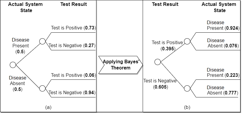
Figure S2.1: Decision tree for the frog conservation problem. The left side (panel (a)) graphically describes probabilities $p(s)$ of disease presence/absence at the new site and probabilities $p(x|s)$ of test results conditional on disease presence/absence. The right side (panel (b)) graphically describes probabilities $p(x)$ of the test returning positive/negative results and probabilities $p(s|x)$ of disease presence/absence conditional on the test result. Application of Bayes’ theorem (Equation (S2.5)) is used to obtain panel (b) from panel (a).

Usage of Equation (5) requires calculation of conditional expectations of the form $\operatorname{\mathbb{E}}_{s|x}\{\cdot\}$, which in turn requires knowledge of conditional probabilities $p(s|x)$. Conditional probabilities $p(s|x)$ can be obtained from conditional probabilities $p(x|s)$ via Bayes’ theorem, which for discrete states $s_{i}$ and discrete measurement outcomes $x_{j}$ is:

$$p(s_{i}|x_{j})=\dfrac{p(x_{j}|s_{i})\,p(s_{i})}{p(x_{j})},\qquad\mbox{where}\qquad p(x_{j})=\displaystyle\sum_{k}p(x_{j}|s_{k})p(s_{k}).$$ (S2.5)

Tedious application of Equation (S2.5) to Equation (S2.4) yields

$$p(x_{1})=0.395,\qquad p(s_{1}|x_{1})=0.924,\qquad p(s_{2}|x_{1})=0.076,$$

$$p(x_{2})=0.605,\qquad p(s_{1}|x_{2})=0.223,\qquad p(s_{2}|x_{2})=0.777.$$ (S2.6)

This information is represented graphically in the right side of Figure S2.1.

Next, intermediate quantities $\max_{a}\{\operatorname{\mathbb{E}}_{s|x_{1}}[V(a,s)]\}$ and $\max_{a}\{\operatorname{\mathbb{E}}_{s|x_{2}}[V(a,s)]\}$, that are required for calculation of $\text{EV}_{\text{less uncertainty}}$, are obtained from the information present in Table S2.1 and Equation (S2.6):

$$\max_{a}\{\operatorname{\mathbb{E}}_{s|x_{1}}[V(a,s)]\} =\max\left\{\sum_{i=1}^{2}V(a_{1},s_{i})\cdot p(s_{i}|x_{1}),\,\,\sum_{i=1}^{2}V(a_{2},s_{i})\cdot p(s_{i}|x_{1})\right\}$$

$$=\max\left\{55\times 0.924+135\times 0.076,\,\,100\times 0.924+100\times 0.076\right\}$$

$$=100,$$ (S2.7)

$$\max_{a}\{\operatorname{\mathbb{E}}_{s|x_{2}}[V(a,s)]\} =\max\left\{\sum_{i=1}^{2}V(a_{1},s_{i})\cdot p(s_{i}|x_{2}),\,\,\sum_{i=1}^{2}V(a_{2},s_{i})\cdot p(s_{i}|x_{2})\right\}$$

$$=\max\left\{55\times 0.223+135\times 0.777,\,\,100\times 0.223+100\times 0.777\right\}$$

$$=117.2.$$ (S2.8)

Then, combining Equations (5) and (S2.6)-(S2.8), the expected value of the system if the best management action is performed after the test is carried out, $\text{EV}_{\text{less uncertainty}}$, is:

$$\text{EV}_{\text{less uncertainty}}=\,\, \operatorname{\mathbb{E}}_{x}[\max_{a}\{\operatorname{\mathbb{E}}_{s|x}[V(a,s)]\}]$$

$$=\,\, p(x_{1})\,\max_{a}\{\operatorname{\mathbb{E}}_{s|x_{1}}[V(a,s)]\}+p(x_{2})\,\max_{a}\{\operatorname{\mathbb{E}}_{s|x_{2}}[V(a,s)]\}$$

$$=\,\, 0.395\times 100+0.605\times 117.2$$

$$=\,\, 110.4.$$ (S2.9)

Finally, combining Equations (6), (S2.3) and (S2.9), the EVSI for this case study is:

EVSI $$=\text{EV}_{\text{less uncertainty}}-\text{EV}_{\text{uncertainty}}$$

$$=110.4-100$$

$$=10.4.$$ (S2.10)

Therefore, the expected value of the test for disease at the new site is an increase in the total frog population of 10.4 individuals.

S2.2 Further details for calculation of new VoI metrics for Case study 1

In Section 3.1.3 of the main text, we summarised the outputs of new VoI calculations for the first case study of the manuscript (protecting frogs from disease outbreaks). Here we explain how these outputs are calculated from application of Equations (7)-(11) to the case study information provided in Section 3.1.1. We also here make use of quantities already computed in Section S2.1 for the present case study.

Combining Equations (7), (S2.3), (S2.7) and (S2.8), the shifts in expected value of the system, $\Delta\text{EV}_{x_{1}}$ and $\Delta\text{EV}_{x_{2}}$, if measurement outcome $x_{1}$ (test positive for disease) or $x_{2}$ (test negative for disease) are obtained respectively, are:

$$\Delta\text{EV}_{x_{1}} =\max_{a}\{\operatorname{\mathbb{E}}_{s|x_{1}}[V(a,s)]\}-\text{EV}_{\text{uncertainty}}=100-100=0,$$ (S2.11)

$$\Delta\text{EV}_{x_{2}} =\max_{a}\{\operatorname{\mathbb{E}}_{s|x_{2}}[V(a,s)]\}-\text{EV}_{\text{uncertainty}}=117.2-100=17.2.$$ (S2.12)

Using Equation (8), the optimal action under uncertainty $a^{*}$ is $a_{2}$ (do nothing); this can already be seen from Equation (S2.3). Usage of Equation (9) requires the intermediate quantities $\operatorname{\mathbb{E}}_{s|x_{1}}[V(a^{*},s)]$ and $\operatorname{\mathbb{E}}_{s|x_{2}}[V(a^{*},s)]$, which can themselves be calculated from information present in Table S2.1 and Equation (S2.6):

$$\operatorname{\mathbb{E}}_{s|x_{1}}[V(a^{*},s)] =\operatorname{\mathbb{E}}_{s|x_{1}}[V(a_{2},s)]$$

$$=V(a_{2},s_{1})\,p(s_{1}|x_{1})+V(a_{2},s_{2})\,p(s_{2}|x_{1})$$

$$=100\times 0.924+100\times 0.076$$

$$=100,$$ (S2.13)

$$\operatorname{\mathbb{E}}_{s|x_{2}}[V(a^{*},s)] =\operatorname{\mathbb{E}}_{s|x_{2}}[V(a_{2},s)]$$

$$=V(a_{2},s_{1})\,p(s_{1}|x_{2})+V(a_{2},s_{2})\,p(s_{2}|x_{2})$$

$$=100\times 0.223+100\times 0.777$$

$$=100.$$ (S2.14)

Then, combining Equations (9), (S2.7), (S2.8), (S2.13) and (S2.14), the values of sample information VSI${}_{x_{1}}$ and VSI${}_{x_{2}}$ dependent on measurement outcomes $x_{1}$ (test positive for disease) and $x_{2}$ (test negative for disease) respectively, are:

$$\text{VSI}_{x_{1}} =\max_{a}\{\operatorname{\mathbb{E}}_{s|x_{1}}[V(a,s)]\}-\operatorname{\mathbb{E}}_{s|x_{1}}[V(a^{*},s)]=100-100=0,$$ (S2.15)

$$\text{VSI}_{x_{2}} =\max_{a}\{\operatorname{\mathbb{E}}_{s|x_{2}}[V(a,s)]\}-\operatorname{\mathbb{E}}_{s|x_{2}}[V(a^{*},s)]=117.2-100=17.2.$$ (S2.16)

Combining Equations (10), (S2.6), (S2.10), (S2.15) and (S2.16), the standard deviation of the value of sample information, $\sigma\text{VSI}$, is given by:

$$\sigma\text{VSI} =\sqrt{\text{Var}_{x}[\text{VSI}_{x}]}$$

$$=\sqrt{\operatorname{\mathbb{E}}_{x}\left[\left(\text{VSI}_{x}-\operatorname{\mathbb{E}}_{x}\left[\text{VSI}_{x}\right]\right)^{2}\right]}$$

$$=\sqrt{\operatorname{\mathbb{E}}_{x}\left[\left(\text{VSI}_{x}-\text{EVSI}\right)^{2}\right]}$$

$$=\sqrt{p(x_{1})\,\left(\text{VSI}_{x_{1}}-\text{EVSI}\right)^{2}+p(x_{2})\,\left(\text{VSI}_{x_{2}}-\text{EVSI}\right)^{2}}$$

$$=\sqrt{0.395\times(0-10.4)^{2}+0.605\times(17.2-10.4)^{2}}$$

$$=8.4.$$ (S2.17)

Finally, since there is a probability of 0.395 that VSI is zero (from Equations (S2.6) and (S2.15)), and there is a probability of 0.605 that VSI is 17.2 (from Equations (S2.6) and (S2.16)), the risk of the VSI being equal to or less than zero is 0.395. This information, if rewritten using Equation (11), is equivalent to the mathematical statement rVSI${}_{0}=0.395$ discussed in Section 3.1.3 of the main text.

S3 Further details for Case study 2

S3.1 Knowledge of the system prior to any of the proposed trials or measurement actions, for Case study 2

Table S3.1: Values of the system, $V(a,s)$, and prior probabilities $p(s)$, for the turtle reintroduction problem (Case study 2). Information for this table is obtained from Table 3 of Canessa et al. (2015).

		States $s$
Values $V(a,s)$		No post-release	Post-release	Post-release
		effect ($s_{1}$)	effect decreases	effect increases
			with age ($s_{2}$)	with age ($s_{3}$)
	Release 3-	0.689	0.582	0.547
	year olds ($a_{1}$)
Actions $a$	Release 4-	0.729	0.674	0.484
	year olds ($a_{2}$)
	Release 5-	0.745	0.710	0.332
	year olds ($a_{3}$)
Prior probabilities $p(s)$		0.4	0.2	0.4

Table S3.2: Probability $p_{\text{survival}}(d,s)$ that a single turtle will survive in the wild for one year, dependent on the system state $s$ and the turtle’s age at the time of release into the wild (experimental design $d$). Information for this table is obtained from Table 3 of Canessa et al. (2015).

		States $s$
Survival probabilities $p_{\text{survival}}(d,s)$		No post-release	Post-release	Post-release
for a single turtle,		effect ($s_{1}$)	effect decreases	effect increases
one year in the wild			with age ($s_{2}$)	with age ($s_{3}$)
	Release 3-	0.85	0.72	0.68
Proposed one-year	year olds ($d_{1}$)
trial release,	Release 4-	0.90	0.83	0.60
according to	year olds ($d_{2}$)
experimental design $d$	Release 5-	0.90	0.86	0.40
	year olds ($d_{3}$)

S3.2 Additional results for Case Study 2

Table S3.3: Probabilities of system state dependent on measurement outcome, $p(x|s)$, of the third proposed experimental design ($d_{3}$: release 5-year old turtles for one year) in the second case study of improving survival of turtles released from captivity (see Section 3.2 for case study details). Upward-pointing arrows ($\uparrow$) and downward-pointing arrows ($\downarrow$) highlight the increase or decrease, respectively, in the probability of the associated system state $s$ due to measurement outcome $x$, compared with the prior belief of this system state: $p(s_{1})=0.4$, $p(s_{2})=0.2$ and $p(s_{3})=0.4$, as shown in Table S3.1.

Experimental design $d_{3}$: One-year trial release of 5-year old turtles
Number of	Probability of	Probability $p(s|x)$ of system state $s$ if outcome $x$ is obtained
surviving	measurement	No post-release	Post-release effect	Post-release effect
turtles, $x$	outcome, $p(x)$	effect ($s_{1}$)	decreases with age ($s_{2}$)	increases with age ($s_{3}$)
0	0.0024	0.0000 ($\downarrow$)	0.0000 ($\downarrow$)	1.0000 ($\uparrow$)
1	0.0161	0.0000 ($\downarrow$)	0.0000 ($\downarrow$)	1.0000 ($\uparrow$)
2	0.0484	0.0000 ($\downarrow$)	0.0000 ($\downarrow$)	1.0000 ($\uparrow$)
3	0.0860	0.0000 ($\downarrow$)	0.0002 ($\downarrow$)	0.9998 ($\uparrow$)
4	0.1006	0.0005 ($\downarrow$)	0.0017 ($\downarrow$)	0.9977 ($\uparrow$)
5	0.0821	0.0072 ($\downarrow$)	0.0155 ($\downarrow$)	0.9772 ($\uparrow$)
6	0.0556	0.0803 ($\downarrow$)	0.1174 ($\downarrow$)	0.8022 ($\uparrow$)
7	0.0629	0.3652 ($\downarrow$)	0.3645 ($\uparrow$)	0.2702 ($\downarrow$)
8	0.1345	0.5760 ($\uparrow$)	0.3924 ($\uparrow$)	0.0316 ($\downarrow$)
9	0.2276	0.6807 ($\uparrow$)	0.3165 ($\uparrow$)	0.0028 ($\downarrow$)
10	0.1838	0.7589 ($\uparrow$)	0.2408 ($\uparrow$)	0.0002 ($\downarrow$)

Table S3.4: Calculated values for the new VoI metrics that are dependent on measurement outcomes, alongside the probabilities of these outcomes and corresponding flow-on effects to the recommended management action, for the first proposed experimental design ($d_{1}$: release 3-year old turtles for one year) in the second case study of improving survival of turtles released from captivity (see Section 3.2 for case study details).

Experimental design $d_{1}$: One-year trial release of 3-year old turtles
Number of	Shift in expected	Value of sample	Probability of	Does the recommended
surviving	value of the	information,	measurement	action change after the
turtles, $x$	system, $\Delta\text{EV}_{x}$	$\text{VSI}_{x}$	outcome, $p(x)$	measurement outcome?
0	–0.0689	0.0449	0.0000	Yes, release 3-year olds instead
1	–0.0680	0.0416	0.0001	Yes, release 3-year olds instead
2	–0.0669	0.0377	0.0011	Yes, release 3-year olds instead
3	–0.0653	0.0331	0.0064	Yes, release 3-year olds instead
4	–0.0626	0.0275	0.0252	Yes, release 3-year olds instead
5	–0.0576	0.0204	0.0694	Yes, release 3-year olds instead
6	–0.0476	0.0110	0.1391	Yes, release 3-year olds instead
7	–0.0279	0	0.2105	No, still release 4-year olds
8	0.0135	0	0.2456	No, still release 4-year olds
9	0.0544	0	0.2079	No, still release 4-year olds
10	0.0854	0.0026	0.0947	Yes, release 5-year olds instead

Table S3.5: Probabilities of system state dependent on measurement outcome, $p(x|s)$, of the first proposed experimental design ($d_{1}$: release 3-year old turtles for one year) in the second case study of improving survival of turtles released from captivity (see Section 3.2 for case study details). Upward-pointing arrows ($\uparrow$) and downward-pointing arrows ($\downarrow$) highlight the increase or decrease, respectively, in the probability of the associated system state $s$ due to measurement outcome $x$, compared with the prior belief of this system state: $p(s_{1})=0.4$, $p(s_{2})=0.2$ and $p(s_{3})=0.4$, as shown in Table S3.1.

Experimental design $d_{1}$: One-year trial release of 3-year old turtles
Number of	Probability of	Probability $p(s|x)$ of system state $s$ if outcome $x$ is obtained
surviving	measurement	No post-release	Post-release effect	Post-release effect
turtles, $x$	outcome, $p(x)$	effect ($s_{1}$)	decreases with age ($s_{2}$)	increases with age ($s_{3}$)
0	0.0000	0.0005 ($\downarrow$)	0.1162 ($\downarrow$)	0.8834 ($\uparrow$)
1	0.0001	0.0012 ($\downarrow$)	0.1372 ($\downarrow$)	0.8617 ($\uparrow$)
2	0.0011	0.0030 ($\downarrow$)	0.1610 ($\downarrow$)	0.8359 ($\uparrow$)
3	0.0064	0.0078 ($\downarrow$)	0.1875 ($\downarrow$)	0.8046 ($\uparrow$)
4	0.0252	0.0198 ($\downarrow$)	0.2156 ($\uparrow$)	0.7646 ($\uparrow$)
5	0.0694	0.0490 ($\downarrow$)	0.2420 ($\uparrow$)	0.7090 ($\uparrow$)
6	0.1391	0.1153 ($\downarrow$)	0.2586 ($\uparrow$)	0.6261 ($\uparrow$)
7	0.2105	0.2467 ($\downarrow$)	0.2510 ($\uparrow$)	0.5023 ($\uparrow$)
8	0.2456	0.4494 ($\uparrow$)	0.2075 ($\uparrow$)	0.3431 ($\downarrow$)
9	0.2079	0.6685 ($\uparrow$)	0.1401 ($\downarrow$)	0.1914 ($\downarrow$)
10	0.0947	0.8316 ($\uparrow$)	0.0791 ($\downarrow$)	0.0893 ($\downarrow$)

Table S3.6: Calculated values for the new VoI metrics that are dependent on measurement outcomes, alongside the probabilities of these outcomes and corresponding flow-on effects to the recommended management action, for the second proposed experimental design ($d_{2}$: release 4-year old turtles for one year) in the second case study of improving survival of turtles released from captivity (see Section 3.2 for case study details).

Experimental design $d_{2}$: One-year trial release of 4-year old turtles
Number of	Shift in expected	Value of sample	Probability of	Does the recommended
surviving	value of the	information,	measurement	action change after the
turtles, $x$	system, $\Delta\text{EV}_{x}$	$\text{VSI}_{x}$	outcome, $p(x)$	measurement outcome?
0	–0.0730	0.0630	0.0000	Yes, release 3-year olds instead
1	–0.0730	0.0630	0.0006	Yes, release 3-year olds instead
2	–0.0730	0.0628	0.0043	Yes, release 3-year olds instead
3	–0.0729	0.0625	0.0170	Yes, release 3-year olds instead
4	–0.0725	0.0612	0.0451	Yes, release 3-year olds instead
5	–0.0708	0.0570	0.0837	Yes, release 3-year olds instead
6	–0.0641	0.0438	0.1163	Yes, release 3-year olds instead
7	–0.0419	0.0110	0.1410	Yes, release 3-year olds instead
8	0.0273	0	0.1844	No, still release 4-year olds
9	0.0871	0.0099	0.2347	Yes, release 5-year olds instead
10	0.1129	0.0172	0.1729	Yes, release 5-year olds instead

Table S3.7: Probabilities of system state dependent on measurement outcome, $p(x|s)$, of the second proposed experimental design ($d_{2}$: release 4-year old turtles for one year) in the second case study of improving survival of turtles released from captivity (see Section 3.2 for case study details). Upward-pointing arrows ($\uparrow$) and downward-pointing arrows ($\downarrow$) highlight the increase or decrease, respectively, in the probability of the associated system state $s$ due to measurement outcome $x$, compared with the prior belief of this system state: $p(s_{1})=0.4$, $p(s_{2})=0.2$ and $p(s_{3})=0.4$, as shown in Table S3.1.

Experimental design $d_{2}$: One-year trial release of 4-year old turtles
Number of	Probability of	Probability $p(s|x)$ of system state $s$ if outcome $x$ is obtained
surviving	measurement	No post-release	Post-release effect	Post-release effect
turtles, $x$	outcome, $p(x)$	effect ($s_{1}$)	decreases with age ($s_{2}$)	increases with age ($s_{3}$)
0	0.0000	0.0000 ($\downarrow$)	0.0001 ($\downarrow$)	0.9999 ($\uparrow$)
1	0.0006	0.0000 ($\downarrow$)	0.0003 ($\downarrow$)	0.9997 ($\uparrow$)
2	0.0043	0.0000 ($\downarrow$)	0.0010 ($\downarrow$)	0.9989 ($\uparrow$)
3	0.0170	0.0002 ($\downarrow$)	0.0033 ($\downarrow$)	0.9965 ($\uparrow$)
4	0.0451	0.0012 ($\downarrow$)	0.0107 ($\downarrow$)	0.9881 ($\uparrow$)
5	0.0837	0.0071 ($\downarrow$)	0.0337 ($\downarrow$)	0.9592 ($\uparrow$)
6	0.1163	0.0384 ($\downarrow$)	0.0986 ($\downarrow$)	0.8630 ($\uparrow$)
7	0.1410	0.1629 ($\downarrow$)	0.2270 ($\uparrow$)	0.6101 ($\uparrow$)
8	0.1844	0.4201 ($\uparrow$)	0.3176 ($\uparrow$)	0.2623 ($\downarrow$)
9	0.2347	0.6604 ($\uparrow$)	0.2709 ($\uparrow$)	0.0687 ($\downarrow$)
10	0.1729	0.8066 ($\uparrow$)	0.1795 ($\downarrow$)	0.0140 ($\downarrow$)

References

• Canessa et al. (2015) Canessa, S., Guillera-Arroita, G., Lahoz-Monfort, J.J., Southwell, D.M., Armstrong, D.P., Chadès, I., Lacy, R.C., Converse, S.J., 2015. When do we need more data? A primer on calculating the value of information for applied ecologists. Methods in Ecology and Evolution 6, 1219–1228.