SN 2022crv: IIb, Or Not IIb: That is the Question

Abstract

We present optical and near-infrared observations of SN 2022crv, a stripped envelope supernova in NGC 3054, discovered within 12 hrs of explosion by the Distance Less Than 40 Mpc Survey. We suggest SN 2022crv is a transitional object on the continuum between SNe Ib and SNe IIb. A high-velocity hydrogen feature ($\sim$$-$20,000 – $-$16,000 $\rm km\,s^{-1}$) was conspicuous in SN 2022crv at early phases, and then quickly disappeared around maximum light. By comparing with hydrodynamic modeling, we find that a hydrogen envelope of $\sim 10^{-3}$ $\rm M_{\odot}$ can reproduce the behaviour of the hydrogen feature observed in SN 2022crv. The early light curve of SN 2022crv did not show envelope cooling emission, implying that SN 2022crv had a compact progenitor with extremely low amount of hydrogen. The analysis of the nebular spectra shows that SN 2022crv is consistent with the explosion of a He star with a final mass of $\sim$4.5 – 5.6 $\rm M_{\odot}$ that has evolved from a $\sim$16 – 22 $\rm M_{\odot}$ zero-age main sequence star in a binary system with about 1.0 – 1.7 $\rm M_{\odot}$ of oxygen finally synthesized in the core. The high metallicity at the supernova site indicates that the progenitor experienced a strong stellar wind mass loss. In order to retain a small amount of residual hydrogen at such a high metallicity, the initial orbital separation of the binary system is likely larger than $\sim$1000 $\rm R_{\odot}$. The near-infrared spectra of SN 2022crv show a unique absorption feature on the blue side of He I line at $\sim$1.005 $\mu$m. This is the first time that such a feature has been observed in a Type Ib/IIb, and could be due to Sr II. Further detailed modelling on SN 2022crv can shed light on the progenitor and the origin of the mysterious absorption feature in the near infrared.

1 Introduction

Stripped envelope supernovae (SESNe) are a subclass of core-collapse supernovae (SNe) that have partly or completely lost their progenitor envelope prior to their explosions (see Modjaz et al. 2019 for a recent review). SESNe are spectroscopically classified as SNe IIb, SNe Ib and SNe Ic (Harkness et al., 1987; Wheeler & Harkness, 1990; Filippenko, 1988, 1997; Clocchiatti & Wheeler, 1997) depending on the presence or absence of H and He lines in the optical spectra. SNe Ib show strong He lines but not H lines, while SNe Ic show neither H nor He lines. SNe IIb show clear H lines at early phases, and then the H lines become weaker over time and the spectra would be similar to SNe Ib at late phases. The sequence of SESNe (IIb$\rightarrow$Ib$\rightarrow$Ic) is commonly believed to be a result of differing amounts of stripping of the outer envelopes of their progenitors (Filippenko, 1997; Yoon, 2015; Gal-Yam, 2017; Hiramatsu et al., 2021).

These hydrogen-deficient SN progenitors have been suggested to either arise from massive and metal-rich stars undergoing mass loss via stellar winds (Woosley et al., 1993, 1995, 2002; Eldridge & Tout, 2004; Meynet & Maeder, 2005; Yoon, 2017) or from binary interactions (Podsiadlowski et al., 1992; Woosley et al., 1995; Wellstein & Langer, 1999; Eldridge & Tout, 2004; Fryer et al., 2007; Yoon et al., 2010; Eldridge et al., 2013; Yoon et al., 2010, 2017; Götberg et al., 2018). Due to the high observed rate of SESNe, relatively weak stellar winds, and the small number of very massive stars assuming a Salpeter initial mass function (Salpeter, 1955), most SESNe progenitors likely result from binary interaction (Smith et al., 2011). This has been supported by direct imaging of the progenitor (Aldering et al., 1994; Maund et al., 2004, 2011; Van Dyk et al., 2011; Eldridge et al., 2013; Fremling et al., 2014; Van Dyk et al., 2014; Eldridge et al., 2015; Folatelli et al., 2016; Kilpatrick et al., 2017; Tartaglia et al., 2017; Kilpatrick et al., 2021), X-ray/radio observations (e.g., Wellons et al., 2012; Drout et al., 2016; Brethauer et al., 2022), and relatively low ejecta mass found from SESNe light curves (Drout et al., 2011; Lyman et al., 2016).

With increasing numbers of well-observed SESNe for each subclass, many objects are becoming difficult to classify unambiguously because they are being discovered with overlapping properties. For instance, an absorption feature at around 6200 Å has been found in some SNe Ib and could be attributed to high-velocity $\rm H\alpha$ (Deng et al., 2000; Branch et al., 2002; Elmhamdi et al., 2006; Parrent et al., 2007; Stritzinger et al., 2009; James & Baron, 2010; Stritzinger et al., 2020; Holmbo et al., 2023), indicating these objects may still contain a small amount of hydrogen. However, the hydrogen features detected in these objects could also be due to Si II $\lambda$6355, C II $\lambda$6580 or Ne I $\lambda$6402 (Deng et al., 2000; Branch et al., 2002; Hamuy et al., 2002; Tanaka et al., 2009; Stritzinger et al., 2009; Dessart et al., 2011; Hachinger et al., 2012). Folatelli et al. (2014) identified a small sample of transitional Type Ib/c SNe that seem to shift from Type Ic to Type Ib over time. These objects show initially weak helium features with nearly constant velocities during the photospheric phase, suggesting a dense shell in the ejecta. However, the weak hydrogen features seen in these objects technically result in a peculiar Type IIb classification. Milisavljevic et al. (2013) found that SESN 2011ei showed unambiguous hydrogen features at early times but these features quickly disappeared on a timescale of one week, suggesting the progenitor retained a thin hydrogen envelope at the time of explosion. Such a transformation is much faster than those observed in typical Type IIb SNe, which usually occur on a timescale of months. This implies that some Type IIb SNe may be misclassified as Type Ib SNe if they are not caught early enough.

All these observations point towards a continuum between SNe IIb and SNe Ib, and there even may be some hydrogen hidden in Type Ib SNe, which is also supported by theoretical studies. For instance, Yoon et al. (2010) found that many Type Ib/c SNe progenitors formed in close binary systems are expected to maintain a thin hydrogen layer during their pre-supernova stage, producing the high-velocity hydrogen features observed in SNe Ib. In a series of models with various amounts of hydrogen, Hachinger et al. (2012) found that if the hydrogen envelope mass at the time of core collapse is between about 0.025 and 0.033 $\rm M_{\odot}$, the difference between Type Ib and Type IIb could be unclear.

Although observational evidence has suggested that there is likely a continuum in the amount of helium between SNe IIb and SNe Ib (Liu et al., 2016; Fremling et al., 2018, although see Holmbo et al. 2023), whether SNe IIb and SNe Ib can be clearly differentiated observationally is still an open question. To better characterize the classification of different types of SESNe and thus understand their progenitors, Liu et al. (2016) performed an analyse of a sample of SESNe. They proposed that the strength of $\rm H\alpha$ (or the absorption feature at around 6200 Å) can be used to differentiate SNe Ib and SNe IIb at all epochs. Prentice & Mazzali (2017) reassessed the classification system of SESNe using the spectra of a sample of SESNe and found that there is a clear distinction between He-poor SNe (SNe Ic) and He-rich SNe (SNe Ib/IIb). They attributed the 6200 Å feature in SNe Ib to $\rm H\alpha$ and further suggested that the He-rich SNe can be split into subgroups based on the profile of the $\rm H\alpha$ line. To fully utilize spectra taken of SESNe, Williamson et al. (2019) proposed a new classification technique based on a support vector machine (SVM). This technique can identify transitional SESNe, i.e., SNe that present spectral features resembling more than one SESNe subtype, and thus reflects the physical properties of their progenitors. These sample studies imply the presence of a gradual transition between Type Ib SNe and Type IIb SNe depending on the amount of hydrogen remaining in the progenitor envelope.

To better understand the connections between the different SESNe types and the evolution of their progenitors, a sample of SESNe that retain a small amount of hydrogen envelope is required. These objects need to be discovered shortly after the explosion since only the very early spectra convey signals from the outer layer of the progenitor star. In this paper, we present optical and infrared data of SN 2022crv, a SESN discovered within $\sim$12 hrs of explosion by the Distance Less Than 40 Mpc (DLT40, Tartaglia et al., 2018) survey and densely monitored for over one year. A hydrogen feature is detected in SN 2022crv at early phases and then quickly disappear shortly after the maximum. Detailed analyses suggest that there is very little hydrogen in the SN envelope, making the object a transitional object on the continuum between SNe Ib and SNe IIb.

This paper is organized as follows: the observations of SN 2022crv are presented in Section 2, while the observational properties, such as the reddening, distance and explosion epoch are constrained in Section 3. We describe the photometric and spectroscopic properties of SN 2022crv in Section 4 and 5, respectively. The physical implications of the observations are discussed in Section 6, and finally we conclude in Section 7.

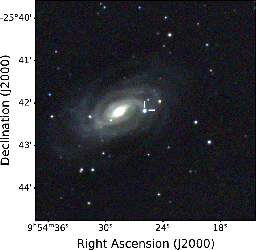
Figure 1: Composite $gri$ image of SN 2022crv in NGC3054 obtained with the Las Cumbres Observatory on 2022 March 04. The position of SN 2022crv is indicated by white tick markers.

Table 1: Basic properties of SN 2022crv

Host galaxy	NGC 3054
RA (2000)	09h54m25$\fs$91
DEC (2000)	$-25\arcdeg 42\arcmin 11\farcs 16$
Distance	$31.6_{-5.3}^{+6.4}$ Mpc
Distance modulus	$32.5\pm 0.4$ mag
Redshift	0.008091$\pm$0.000023
$E(B-V)_{\rm MW}$	$0.0642_{-0.007}^{+0.007}$ mag*
$E(B-V)_{\rm host}$	$0.146_{-0.009}^{+0.009}$ mag
Explosion epoch (JD)	$2459627.19\pm 0.30$ (2022-02-16)
$V_{\rm max}$ (JD)	2459645.42 (2022-03-06)

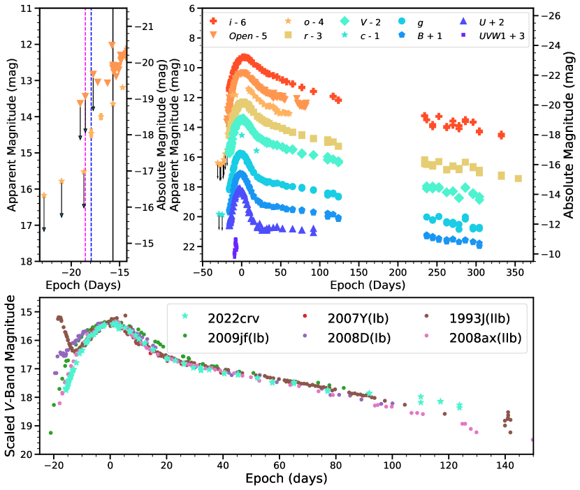
Figure 2: Upper right: Multiband light curves for SN 2022crv with respect to the $V$-band maximum (JD 2459645.42). The DLT40 $Open$ filter light curve is calibrated to the $r$ band. Upper left: A zoom around a few days before and after the discovery. Only the $Open$- and $o$-band light curves are plotted here to show the constraint on the explosion epoch. The last nondetection and the earliest detection are marked by the magenta vertical dashed line and blue vertical dashed line, respectively. The black vertical line marks when the multiband followup began. Bottom: The $V$-band light curve of SN 2022crv compared to other SESNe. The magnitudes of other objects have been scaled to match the peak of SN 2022crv. The data used to create this figure are available.

2 Observations

SN 2022crv/DLT22d was discovered at RA(2000) $=$ 09^h54^m25$\fs$91, Dec(2000) $=-25\arcdeg 42\arcmin 11\farcs 16$ in the nearby barred spiral (SBc) galaxy NGC 3054 (see Figure 1) on 2022-02-17.20 (Dong et al. 2022, JD 2459627.696, $r$ = 18.04), during the course of the DLT40 SN search (Tartaglia et al., 2018), utilizing the 0.4-m PROMPT-MO-1 telescope (Reichart et al., 2005) at the Meckering Observatory. An earlier detection was recovered in the $o$-band imaging taken by the Asteroid Terrestrial-Impact Last Alert System (ATLAS, Tonry 2011; Tonry et al. 2018; Smith et al. 2020) on 2022-02-16.99. The object was initially classified as a Type Ib using a spectrum taken with GMOS on Gemini North on 2022-02-19.42 (Andrews et al., 2022). The basic properties of SN 2022crv are summarized in Table 1.

Table 2: Spectroscopic observations of SN 2022crv.

Phase (Days)$\star$	MJD	Telescope	Instrument	Range (Å)
-15.5/2.7	59629.43	Gemini-N	GMOS	3760-7030
-15.5/2.8	59629.46	KeckII	NIRES	9650-24660
-15.3/2.9	59629.61	FTS	FLOYDS	4850-10170
-15.1/3.1	59629.82	SALT	RSS	3930-7790
-13.4/4.8	59631.49	FTN	FLOYDS	3510-9990
-11.5/6.7	59633.39	FTN	FLOYDS	3510-9990
-10.7/7.5	59634.23	SOAR	Goodman	3780-5460
-10.5/7.8	59634.46	FTN	FLOYDS	3500-9990
-7.6/10.6	59637.34	FTN	FLOYDS	3510-10000
-6.6/11.6	59638.32	LBT	MODS	3400-10100
-6.5/11.8	59638.46	FTN	FLOYDS	3510-9990
-3.5/14.7	59641.43	FTS	FLOYDS	3510-9990
-0.6/17.7	59644.35	FTN	FLOYDS	3500-9990
2.3/20.5	59647.22	Bok	B&C	4010-7490
2.7/21.0	59647.65	FTS	FLOYDS	3500-9990
3.4/21.6	59648.29	LBT	MODS	3610-10290
4.4/22.6	59649.28	FTN	FLOYDS	3500-9990
4.4/22.6	59649.32	UH88	SNIFS	3410-9090
6.2/24.4	59651.07	Baade	FIRE	7910-25250
6.4/24.6	59651.34	FTN	FLOYDS	3500-9990
6.6/24.8	59651.50	Baade	IMACS	4230-9410
7.4/25.7	59652.34	KeckII	NIRES	9650-24660
8.3/26.6	59653.27	KeckII	NIRES	9660-24670
10.4/28.6	59655.30	FTN	FLOYDS	3500-10000
12.1/30.3	59657.00	MMT	MMIRS	9500-24290
12.4/30.6	59657.32	UH88	SNIFS	3410-9090
15.6/33.8	59660.50	Baade	IMACS	4230-9410
15.7/33.9	59660.60	FTS	FLOYDS	3510-9500
17.3/35.6	59662.25	Shane	Kast	3620-10750
18.3/36.5	59663.19	LBT	MODS	3400-9990
19.2/37.5	59664.17	MMT	Binospec	5240-6750
19.3/37.6	59664.25	UH88	SNIFS	3410-9090
24.0/42.2	59668.90	NOT	ALFOSC	3410-9660
24.6/42.8	59669.50	Baade	IMACS	4230-9410
25.3/43.5	59670.21	Shane	Kast	3630-10740
28.6/46.9	59673.57	FTS	FLOYDS	3510-9990
35.4/53.6	59680.28	FTN	FLOYDS	3500-9990
35.4/53.6	59680.29	UH88	SNIFS	3410-9090
36.6/54.8	59681.50	Baade	IMACS	4230-9410
44.6/62.9	59689.54	FTS	FLOYDS	3500-10000
48.4/66.6	59693.29	UH88	SNIFS	3410-9090
50.3/68.6	59695.24	KeckI	LRIS	3150-5640
50.3/68.6	59695.24	KeckI	LRIS	5420-10300
50.3/68.6	59695.25	KeckI	LRIS	5490-7140
54.9/73.2	59699.86	SALT	RSS	3930-7790
56.5/74.7	59701.42	FTS	FLOYDS	3500-10000
58.2/76.5	59703.15	LBT	MODS	3720-10000
64.4/82.6	59709.29	KeckII	NIRES	9660-24670
69.3/87.6	59714.25	KeckII	NIRES	9650-24670
70.3/88.6	59715.25	KeckII	NIRES	9660-24670
71.5/89.7	59716.43	FTS	FLOYDS	3500-9990
99.5/117.7	59744.41	FTS	FLOYDS	4010-10000
102.8/121.0	59747.73	SALT	RSS	3930-7790
267.4/285.6	59912.29	SOAR	Goodman	3500-7130
272.3/290.6	59917.27	SOAR	Goodman	5000-9000
321.0/339.2	59965.90	SALT	RSS	5480-8990
353.2/371.4	59998.14	Clay	LDSS3	4000-10000
355.1/373.3	60000.03	GTC	OSIRIS	4000-10000

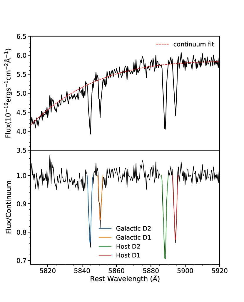
Figure 3: Top: A high-resolution spectrum taken with LRIS on 2022-04-26 (MJD 59695.25) showing the Na I D lines from the host galaxy and the Milky Way. The continuum is fitted with a 4th order polynomial function. Bottom: The continuum-subtracted spectrum. The Na I D lines are fitted with Gaussian functions using a MCMC routine.

After the discovery, the object was intensely followed by the DLT40 survey using PROMPT5 and PROMPT-MO telescopes in the Open filter and the ATLAS survey in the o and c filters. In addition, high-cadence multiband photometric observations were collected by the world-wide network of robotic telescopes of Las Cumbres Observatory (Brown et al., 2013) through the Global Supernova Project. Ultraviolet and optical imaging was taken with the Neil Gehrels Swift Observatory (Gehrels et al., 2004) at early times. The object was also followed by the Katzman Automatic Imaging Telescope (KAIT) as part of the Lick Observatory Supernova Search (LOSS; Filippenko et al., 2001), and the 1 m Nickel telescope at Lick Observatory. B, V, R and I multiband images of SN 2022crv were obtained with both telescopes, additional clear band (close to the R band; see Li et al. 2003) images were also obtained with KAIT. The multiband light curves are shown in Figure 2. The reduction process of the photometric data is presented in Appendix A.

Nineteen low-resolution optical spectra were collected with the FLOYDS spectrograph (Brown et al., 2013) on the 2m Faulkes Telescopes South and North (FTS & FTN) through the Global Supernova Project. In addition, many optical spectra were also obtained with the Robert Stobie Spectrograph (RSS) on the Southern African Large Telescope (SALT; Smith et al., 2006), the Kast Spectrograph on the 3m Shane Telescope (Miller & Stone, 1994) at Lick Observatory, the Boller & Chivens Spectrograph (B&C) on the Bok Telescope (Green et al., 1995), one of the Multi-Object double Spectrographs (MODS1, Pogge et al., 2010) on LBT, the Binospec instrument on the MMT (Fabricant et al., 2019), the Goodman High Throughput Spectrograph on the Southern Astrophysical Research Telescope (SOAR; Clemens et al., 2004), the Low-Resolution Imaging Spectrometer (LRIS; Oke et al., 1995) on the Keck I telescope, the Gemini Multi-Object Spectrograph (GMOS; Hook et al., 2004) on the Gemini North telescope, the Andalucia Faint Object Spectrograph and Camera (ALFOSC) on the Nordic Optical Telescope (NOT) as part of the NUTS2 collaboration, the SuperNova Integral Field Spectrograph (SNIFS; Lantz et al., 2004) mounted at the University of Hawaii 2.2 m telescope (UH88) at Mauna Kea as part of the Spectroscopic Classification of Astronomical Transients survey (SCAT; Tucker et al., 2022), the Inamori-Magellan Areal Camera & Spectrograph (IMACS; Dressler et al., 2011) on the 6.5m Magellan Baade telescope as part of the Precision Observations of Infant Supernova Explosions (POISE; Burns et al., 2021), the the Optical System for Imaging and low/intermediate-Resolution Integrated Spectroscopy (OSIRIS; Cepa et al., 2000) spectrograph on the 10.4 m Gran Telescopio Canarias (GTC), and the Low-Dispersion Survey Spectrograph 3 (LDSS3, which was updated from LDSS2; Allington-Smith et al., 1994) on the 6.5m Magellan Clay telescope.

Near-infrared (NIR) spectra were taken with the Near-Infrared Echellette Spectrometer (NIRES; Wilson et al., 2004) on the Keck II telescope, the Folded-port InfraRed Echellette (FIRE; Simcoe et al., 2013) on Magellan Baade telescope, and the MMT and Magellan Infrared Spectrograph (MMIRS) on the MMT (McLeod et al., 2012).

A log of the spectroscopic observations is given in Table 2. The reduction process for the spectroscopic data is presented in Appendix B.

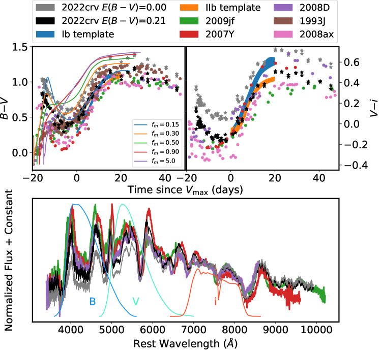
Figure 4: Top: Color evolution of SN 2022crv, after correcting for a total color excess of $E(B-V)$ = 0.21 mag. The color templates from Stritzinger et al. (2018) and a sample of Ib/IIb SNe after correcting with the published reddening estimates are also plotted. The $B-V$ color evolution is also compared with the SNe Ib color evolution models by Yoon et al. (2019) with various degrees of $\rm{}^{56}Ni$ (indicated by $\rm f_{m}$). SN 2022crv is more consistent with the $\rm f_{m}$=0.15/0.3 model, suggesting a relatively weak ⁵⁶Ni mixing in the ejecta (see Section 4). Bottom: Spectral comparison between a sample of Type Ib SNe and SN 2022crv at about 10 days after the $V$-band maximum. The transmission curve for the $B$, $V$, and $i$ bands have been plotted to indicate their wavelength ranges. The grey line shows the spectrum of 2022crv without reddening correction. An $E(B-V)=0.21$ gives a consistent spectrum profile with other objects.

3 Observational Properties

3.1 Explosion Epoch

By combining the early light curves from the DLT40 and the ATLAS surveys, we are able to put a strong constraint on the explosion date of SN 2022crv. The SN was not detected during the DLT40 search on JD 2459626.89 (with a 3$\sigma$ limit of 18.44 mag) On JD 2459627.49, $\sim$14.4 hours after our non-detection, the SN is detected in the $o$-band ATLAS image. The first detection and the last non-detection of SN 2022crv are highlighted in the left panel of Figure 2. By taking the average between the first detection and the last non-detection, we constrain the explosion epoch to be JD 2459627.19$\pm$0.30, which will be adopted throughout the paper.

3.2 Reddening Estimation

The equivalent width (EW) of the Na I D line is often used to estimate the SN reddening with the assumption that it is a good tracer of the amount of gas and dust (e.g., Munari & Zwitter, 1997; Poznanski et al., 2012). In order to measure the line-of-sight reddening towards SN 2022crv, we analyzed the medium-resolution spectrum (R$\sim$4000) taken with LRIS on 2022-04-26 (Figure 3). We apply a 4th-order polynomial to fit the continuum, and measure the EW of the Na I D lines on the continuum-subtracted spectrum (Figure 3 bottom panel). The measured EW of the host galaxy Na I D $\lambda$5890 ($\rm D_{2}$) and Na I D $\lambda$5896 ($\rm D_{1}$) are $0.544_{-0.012}^{+0.012}$ Å and $0.378_{-0.011}^{+0.011}$ Å, respectively. The measured EW of the Galactic Na I $\rm D_{2}$ and Na I $\rm D_{1}$ are $0.404_{-0.011}^{+0.011}$ Å and $0.247_{-0.011}^{+0.011}$ Å respectively. Using Eq.9 in Poznanski et al. (2012) and applying the renormalization factor of 0.86 from Schlafly et al. (2010), we found a host extinction of $E(B-V)_{\rm host}=0.146_{-0.009}^{+0.009}$ mag with 20% systematic uncertainty (Poznanski et al., 2012). The Milky Way extinction is measured to be $E(B-V)_{\rm MW}=0.070_{-0.004}^{+0.004}$ mag, consistent with the value from (Schlafly & Finkbeiner, 2011), $E(B-V)_{\rm MW}$ = 0.0642 (0.0007) mag. The latter will be adopted in this paper.

For SESNe, the intrinsic color shortly after the maximum light is found to be tightly distributed, both observationally (Drout et al., 2011; Taddia et al., 2015; Stritzinger et al., 2018) and theoretically (Dessart et al., 2016; Woosley et al., 2021). By studying a sample of SESNe, Drout et al. (2011) and Stritzinger et al. (2018) found that, compared to other phases, the scatter in various color indices for each sub-type of SESNe is smaller shortly after the maximum. Based on the modeling of a range of SESNe, Woosley et al. (2021) confirmed that there are pinches in color indices shortly after the peak. They also found that the spectra of SESNe are similar to each other approximately 10 days after the peak. In the top panel of Figure 4, we compare the B$-$V and V$-$i evolution of SN 2022crv with other well-studied SNe Ib/IIb, including SN 2009jf (Valenti et al., 2011; Sahu et al., 2011), SN 2007Y (Stritzinger et al., 2009), SN 2008D (Modjaz et al., 2009), SN 1993J (Filippenko et al., 1993), and SN 2008ax (Pastorello et al., 2008). The color templates for SNe Ib and IIb from Stritzinger et al. (2018) are also plotted. We found that a total extinction of $E(B-V)$=0.21 mag gives SN 2022crv a consistent color evolution with our comparitive sample of SNe Ib/IIb and templates shortly after $V_{\rm max}$. In the bottom panel of Figure 4, we compare the spectrum of SN 2022crv with our other SNe Ib/IIb at around 10 days after $V_{\rm max}$. The original spectrum of SN 2022crv is redder than those of our other objects, while a total extinction of $E(B-V)=\,0.21$ mag gives a spectral slope more consistent with the population. Therefore, throughout this paper, we will adopt an $E(B-V)_{\rm tot}=0.21$ mag, assuming a $\rm R_{V}$ = 3.1.

3.3 Distance

The distance of NGC 3054 listed on the NASA/IPAC Extragalactic Database (NED) ranges from 12.9 Mpc to 40.0 Mpc. SN 2006T (Type IIb; Monard, 2006) also exploded in NGC 3054, and Lyman et al. (2016) used a distance of 32.9 Mpc for SN 2006T, while Taddia et al. (2018) adopted a distance of 31.6 Mpc. To be consistent with the distance of SN 2006T used by previous works, we assume a distance of 31.6${}^{+6.4}_{-5.3}$ Mpc (a distance modulus of 32.5$\pm$0.4 mag) based on the Tully-Fisher distance (Tully et al., 2009).

3.4 Host Properties

SN2022crv is at a projected offset of 36$\farcs$4 (5.6${}^{+1.1}_{-0.9}$ kpc) from the host galaxy NGC 3054. To estimate the metallicity at the SN position, we measured the flux of the strong ionized gas emission lines (H$\beta$, O III] $\lambda$5007, [N III] $\lambda$6584, H$\alpha$, [S II] $\lambda\lambda$6717, 6731) from the spectrum taken 371.5 days after the SN explosion. The continuum is removed by fitting a linear component around the narrow emission lines. By using the strong-line diagnostics presented in Curti et al. (2020), the weighted average oxygen abundance at the SN site is measured to be 12 + log(O/H) = 8.83$\pm$0.08 and the results for each indicator calibration are shown in Table 3. Assuming a solar oxygen abundance of 12 + log(O/H) = 8.69 (Allende Prieto et al., 2001) as well as a solar metallicity ($\rm Z_{\odot}$) of 0.0134 (Asplund et al., 2009), 12 + log(O/H) = 8.83 is equivalent to a metallicity of Z $\simeq$ 1.4 $\rm Z_{\odot}\simeq 0.019$. The $\rm O_{3}N_{2}$ calibration indicator in Pettini & Pagel (2004) gives 12 + log(O/H) = 8.88$\pm$0.14, consistent with our measurements above. Comparing to all the SESNe in the PMAS/PPak Integral-field Supernova Hosts Compilation (PISCO) sample (Galbany et al., 2018), SN 2022crv has one of the most metal-rich environments among the Type Ib/IIb SNe in the sample. Given the high metallicity, the progenitor star of SN 2022crv likely experienced strong wind mass loss (Vink et al., 2001; Crowther, 2007; Mokiem et al., 2007). Just before completing our paper, there is another paper on SN 2022crv coming out (Gangopadhyay et al., 2023), and they found a high progenitor mass-loss rate based on the radio light curve, consistent with what we suggested here. The implication of the high mass loss rate will be further discussed in Section 6.3.2.

Table 3: The flux of ionized gas emission lines at the SN position measured from the spectrum taken on 2023-03-23 (371 days after the explosion). The oxygen abundance values are calculated based on the strong-line diagnostics presented in Curti et al. (2020).

Indicator	Line Ratio	Value	12+log[O/H]
R3	[O III] $\lambda$5007/H$\beta$	0.13	8.84$\pm$0.07
N2	[N III] $\lambda$6584/H$\alpha$	0.39	8.75$\pm$0.10
S2	[S II] $\lambda\lambda$6717, 6731/H$\alpha$	0.18	8.87$\pm$0.06
RS_32	[O III] $\lambda$5007/H$\beta$ + [S II] $\lambda$6717, 6731/H$\alpha$	0.31	8.85$\pm$0.08
O_3S_2	([O III] $\lambda$5007/H$\beta$) / ([S II] $\lambda\lambda$6717, 6731/H$\alpha$)	0.72	8.76$\pm$0.11
O_3N_2	([O III] $\lambda$5007/H$\beta$) / ([N II] $\lambda$6584/H$\alpha$)	0.34	8.84$\pm$0.09
Weighted Average			8.83$\pm$0.08

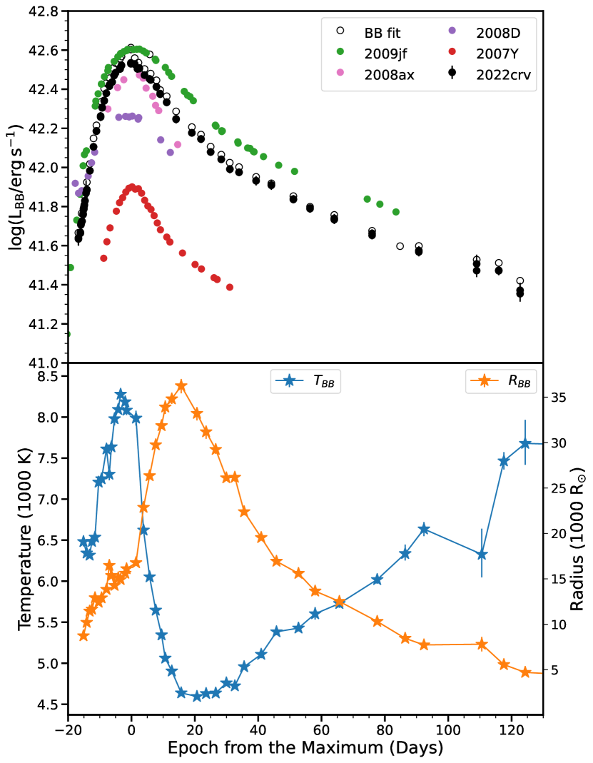
Figure 5: Top: Bolometric light curve of SN 2022crv compared with other Type Ib/IIb SNe. The unfilled points represent the bolometric light curve from the blackbody fit. Bottom: The evolution of temperature and radius of SN 2022crv derived from the blackbody fit.

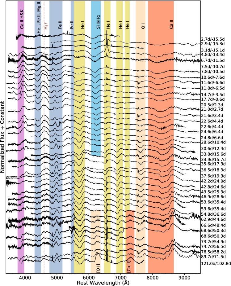
Figure 6: The optical spectroscopic evolution of SN 2022crv from the photospheric phase to the early nebular phase. The phase is measured from the explosion/$V$-band maximum.

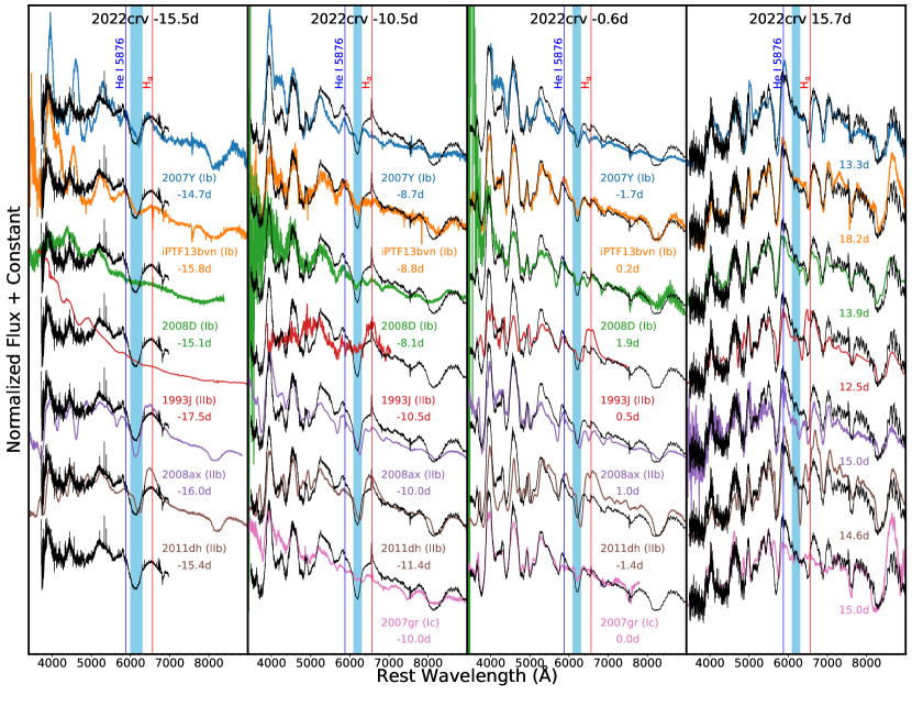
Figure 7: Optical spectral comparison of SN 2022crv to other well-studied SESNe, including SNe Ib, SN 2007Y, iPTF13bvn, SN 2008D; SNe IIb, SN 1993J, SN 2008ax, SN 2011dh; and SNe Ic, SN 2007gr. The blue shaded areas mark the 6200 Å features.

4 photometric evolution

4.1 Light Curve Evolution

The multiband light curves of SN 2022crv are shown in Figure 2. SN 2022crv reaches a V-band maximum of $M_{V}$ = $-$17.7$\pm$0.4 mag on JD 2459645.42, $\sim$18.2 days after the date of explosion. Around 60 days after $V_{\rm max}$, the light curves show a linear decline. The $V$-band decline rate is about 1.4 $\rm mag\,(100d)^{-1}$, faster than the expected radioactive decay rate of $\rm{}^{56}Co\rightarrow{}^{56}Fe$ [0.98 $\rm mag\,(100d)^{-1}$] (Nadyozhin, 1994), which is consistent with other SNe Ib/IIb. In the bottom panel of Figure 2, we compare the $V$-band light curve of SN 2022crv with those of other well-studied SNe Ib/IIb (i.e., SN 2009jf (Valenti et al., 2011), SN 2007Y (Stritzinger et al., 2009), SN 2008D (Modjaz et al., 2009), SN 1993J (Filippenko et al., 1993), SN 2008ax (Pastorello et al., 2008)). The apparent magnitudes of other SESNe in the sample have been shifted to match the peak of SN 2022crv. SN 2022crv does not show an initial peak due to shock cooling like SN 1993J does and has a faster rise than SN 2008D. Overall, the light curve shape of SN 2022crv is similar to SN 2009jf, SN 2007Y and SN 2008ax.

Chevalier & Soderberg (2010) suggested that Type IIb SNe can be divided into two categories according to whether the progenitor is compact or extended. If the amount of hydrogen is low enough, the compact Type IIb would merge into Type Ib. Due to the lack of cooling envelope emission, SN 2022crv likely has a compact progenitor, which will be further discussed in Section 6.2.

The $B-V$ and $V-i$ color evolution of SN 2022crv is compared to our sample of SNe Ib/IIb in Figure 4. The color evolution of SN 2022crv after $V_{max}$ is similar to those of other SESNe in comparison. After correcting for reddening, the $B-V$ color of SN 2022crv shows a rapid initial rise and reaches a peak of $\sim$0.8 mag. The color then evolves toward the blue down to $\sim$0.4 mag. After maximum light, the $B-V$ color increases and reaches a peak of $\sim$1.1 mag before entering the nebular phase. The $V-i$ color of SN 2022crv shows a similar trend. Through hydrodynamical simulations, Yoon et al. (2019) found that the early color evolution of SNe Ib/c is strongly affected by the $\rm{}^{56}Ni$ mixing level in the SN ejecta. The $\rm{}^{56}Ni$ mixing level is characterized by $\rm f_{m}$ in Yoon et al. (2019), with a larger value of $\rm f_{m}$ representing a more mixing. The $B-V$ evolution of SN 2022crv matches with the $\rm f_{m}=0.15$ or the $\rm f_{m}=0.3$ model presented in Yoon et al. (2019) (Figure 4), implying weak $\rm{}^{56}Ni$ mixing in SN 2022crv.

4.2 Bolometric Light Curve

In this section, we build the bolometric light curve of SN 2022crv, which will be used to determine the physical parameters of explosion in Section 6.3.3.

Due to the lack of photometric coverage in the UV and NIR, we calculated the bolometric correction based on the $B-i$ color evolution and applied it to the $B$-band light curve, as described in Lyman et al. (2014, 2016). The bolometric magnitudes are converted to bolometric luminosity assuming $M_{Bol,\,\odot}$ = 4.74 and $L_{Bol,\,\odot}$ = 3.9$\times 10^{33}$ $\rm erg\,s^{-1}$. The bolometric light curve of SN 2022crv is shown in Figure 5 along with those of a sample of Type Ib/IIb SNe. The peak bolometric luminosity of SN 2022crv is 3.39$\rm\times 10^{42}erg\,s^{-1}$ and is almost as bright as SN 2009jf, which puts SN 2022crv on the brighter end among the Type Ib/IIb SNe (Lyman et al., 2016; Taddia et al., 2018; Prentice et al., 2019). As a sanity check, we also calculated the bolometric light curve by fitting the reddening-corrected SED of SN 2022crv with a blackbody spectrum at each epoch using a Markov Chain Monte Carlo (MCMC) routine in the Light Curve Fitting package (Hosseinzadeh & Gomez, 2020). The blackbody bolometric light curve is plotted in Figure 5 and is consistent with the bolometric light curve derived from bolometric correction.

From the blackbody fits, we also derived the radius and temperature evolution of SN 2022crv (bottom panel of Figure 5). The temperature increases after a rapid initial drop at early phases, and reaches a peak of $\sim 8000\,$K several days before $V_{max}$, then it rapidly decreases until reaching a minimum of $\sim 4500\,$K before the object settles into the nebular phase. The behaviour of the temperature evolution is consistent with the color evolution shown in Figure 4. The radius of SN 2022crv continuously increases until it peaks at around 20 days after $V_{\rm max}$. The radius and temperature evolution of SN 2022crv is similar to other SESNe (Taddia et al., 2018).

Table 4: Position of the minimum of the absorption component of the P-cygni profile (Å).

Epoch	MJD	$\rm H{\alpha}$/Si II $\lambda$6355	He I $\lambda$5876	He I $\lambda$6678	Fe II $\lambda$4561	Fe II $\lambda$5018	Fe II $\lambda$5169
2.7	59629.4	6172.5	5623.7	$\cdots$	$\cdots$	$\cdots$	$\cdots$
2.9	59629.6	6183.5	5590.9	$\cdots$	$\cdots$	$\cdots$	$\cdots$
3.1	59629.8	6177.0	5638.5	$\cdots$	$\cdots$	$\cdots$	$\cdots$
4.8	59631.5	6218.0	5678.4	$\cdots$	$\cdots$	$\cdots$	$\cdots$
6.7	59633.4	6237.1	5709.2		4378.0	4814.7	4997.8
7.5	59634.2	$\cdots$	$\cdots$	$\cdots$	4397.2	4842.4	5014.6
7.8	59634.5	6240.0	5657.1		4400.2	4843.7	5014.8
10.6	59637.3	6246.9	5725.6	6500.2	4418.3	4856.7	5020.4
11.6	59638.3	$\cdots$	$\cdots$	$\cdots$	4419.6	4859.1	5025.3
11.6	59638.3	6252.2	$\cdots$	6503.2	$\cdots$	$\cdots$	$\cdots$
11.8	59638.5	6247.9	5730.6	6513.6	4417.4	4857.0	5029.8
14.7	59641.4	6253.6	5769.5	6516.0	4428.1	4863.0	5041.3
17.7	59644.3	6261.7	5771.3	6556.0	4436.3	4870.9	5049.0
21.0	59647.6	6271.4	5762.9	6562.6	$\cdots$	$\cdots$	$\cdots$
21.6	59648.3	$\cdots$	$\cdots$	$\cdots$	4438.9	4886.3	5060.6
21.6	59648.3	6279.7	5767.4	6580.3	$\cdots$	$\cdots$	$\cdots$
22.6	59649.3	6280.6	5767.6	6568.9	$\cdots$	$\cdots$	$\cdots$
22.6	59649.3	6290.1	5774.3	6580.0	4440.8	4878.9	5077.2
24.6	59651.3	6288.1	5760.5	6567.7	$\cdots$	$\cdots$	$\cdots$
24.8	59651.5	6289.8	5759.7	6573.8	4438.1	4904.1	5073.3
28.6	59655.3	6303.8	5745.4	6560.9	$\cdots$	4920.3	5088.0
30.6	59657.3	6320.6	5744.5	6563.6	$\cdots$	4927.3	5093.5

Table 5: The position of the flux minimum of the absorption component of the P cygni profile (Å).

Epoch	MJD	He I $\lambda$5876	He I $\lambda$6678	Fe II $\lambda$5018	Fe II $\lambda$5169
33.8	59660.5	5734.7	6549.4	4917.8	5099.7
33.9	59660.6	5738.8	6555.8	4918.7	5105.2
35.6	59662.2	5737.2	6556.6	$\cdots$	5110.8
37.5	59664.2	5743.4	$\cdots$	$\cdots$	$\cdots$
36.5	59663.2	5745.1	6562.7	$\cdots$	$\cdots$
36.5	59663.2	$\cdots$	$\cdots$	$\cdots$	5108.1
37.6	59664.2	5745.6	6566.0	$\cdots$	5102.7
42.2	59668.9	5737.3	6560.8	$\cdots$	5111.2
42.8	59669.5	5739.7	6565.4	$\cdots$	5114.7
43.5	59670.2	5738.8	6565.8	$\cdots$	5114.1
46.9	59673.6	5738.4	6567.1	$\cdots$	5089.6
53.6	59680.3	5743.9	6571.8	$\cdots$	5095.0
53.6	59680.3	5752.6	6582.9	$\cdots$	$\cdots$
54.8	59681.5	5744.9	6576.5	$\cdots$	5116.4
62.9	59689.5	5753.6	6577.4	$\cdots$	5115.5
66.6	59693.3	5763.9	6590.2	$\cdots$	5117.6
68.6	59695.2	$\cdots$	$\cdots$	$\cdots$	5119.2
68.6	59695.2	5757.8	6589.7	$\cdots$	$\cdots$
68.6	59695.2	5756.4	6594.2	$\cdots$	$\cdots$
73.2	59699.9	5756.1	$\cdots$	$\cdots$	5118.7
74.7	59701.4	5755.1	6578.9	$\cdots$	5097.0
76.5	59703.2	$\cdots$	$\cdots$	$\cdots$	5119.2
76.5	59703.2	5755.0	$\cdots$	$\cdots$	$\cdots$
89.7	59716.4	5765.0	6579.4	$\cdots$	$\cdots$
121.0	59747.7	5770.3	$\cdots$	$\cdots$	5119.7

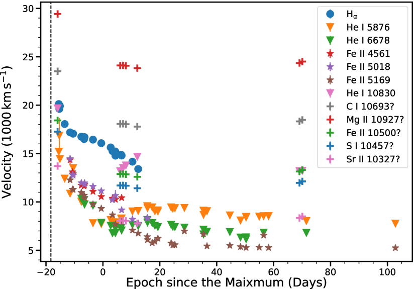
Figure 8: Velocity evolution of $\rm H\alpha$, He I, Fe II and feature A (see Section 5.3). The epoch of explosion is marked with the vertical dashed line. The velocity of feature A is calculated assuming it is from C I $\lambda$1.0693 $\mu$m, Mg I $\lambda$1.0927 $\mu$m, Fe II $\lambda$1.05 $\mu$m, S I $\lambda$1.0457 $\mu$m, and Sr I $\lambda$1.0327 $\mu$m, respectively, and is shown with the plus symbol. The velocity of $\rm H{\alpha}$ shows a rapid drop after the $V_{max}$. As discussed in Section 6.1, the 6200 Å feature is likely dominated by Si II after $V_{\text{max}}$, so this drop does not reliably reflect the velocity evolution of the $\rm H{\alpha}$ line.

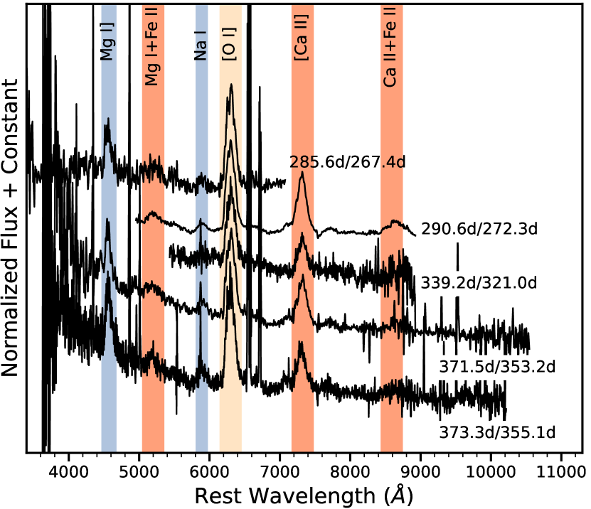
Figure 9: The nebular phase spectroscopic evolution of SN 2022crv. Phase is measured from explosion/$V$-band maximum. All the spectra shown here are smoothed with a second order Savitzky-Golay filter with a window size of 11 Å.

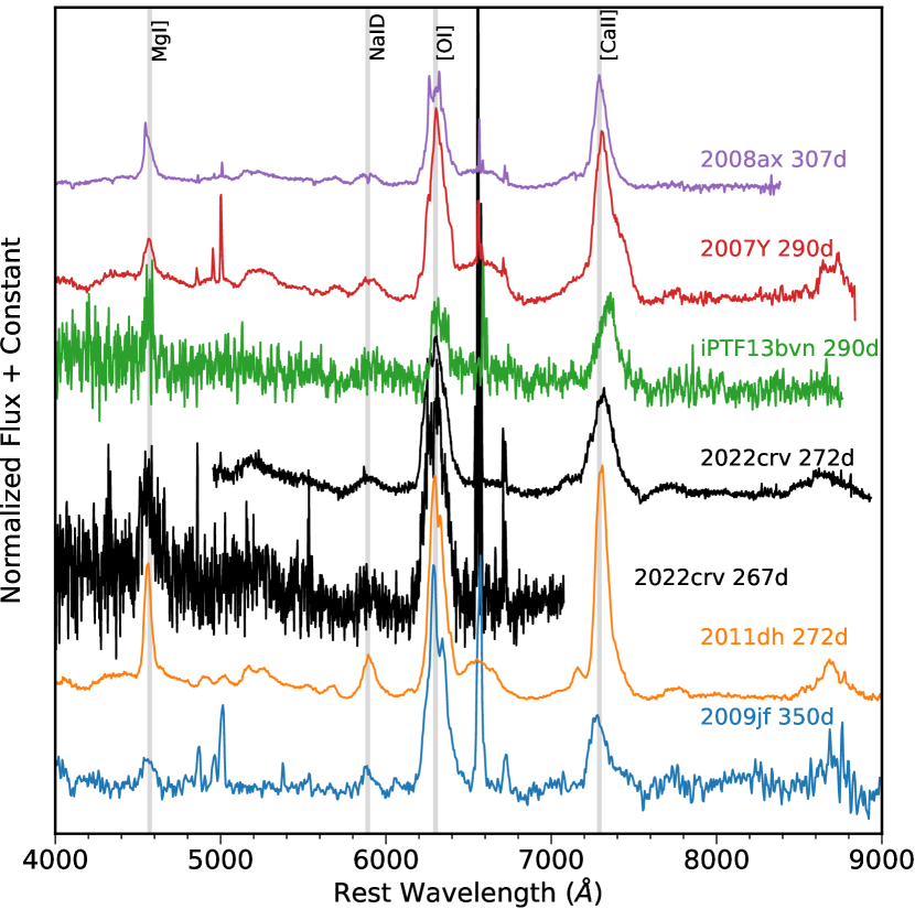
Figure 10: Nebular spectra of SN 2022crv compared to other SESNe. The phase is measured from the $V$-band maximum.

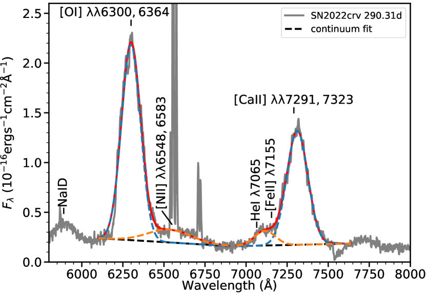
Figure 11: Line identification of the nebular spectrum taken on 2022-12-04. A double Gaussian function is fitted around 6300 Å and 7300 Å, respectively, to deblend the [O I] and [Ca II] from other lines. The continuum is defined by a straight line connecting the two local minima.

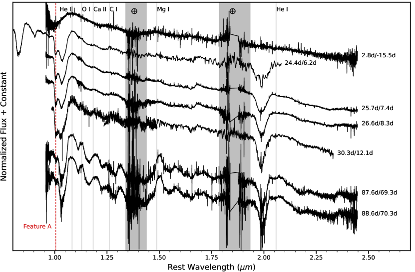
Figure 12: NIR spectra of SN 2022crv. The phase is measured from the explosion/$V$-band maximum. The red dashed line marks the extra absorption feature on the blue side of He I $\lambda$1.083 $\mu$m. The high telluric absorption regions are marked with grey bands.

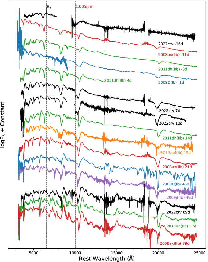
Figure 13: Comparison of combined optical and NIR spectra of SN 2022crv with those of other SNe Ib/IIb. The position of $\rm H{\alpha}$ (black dashed line) and 1.005 $\mu$m (red dashed line) are marked.

Figure 14: Spectral evolution of SN 2022crv in the 1 $\mu$m and 2 $\mu$m regions. The phase if measured from the explosion/$V$-band maximum. Feature A can be fit with a two-Gaussian function. The velocity scales of C I $\lambda$1.0693 $\mu$m, Mg I $\lambda$1.0927 $\mu$m, high velocity (HV) He I $\lambda$1.083 $\mu$m, Fe II $\lambda$1.05 $\mu$m, S I $\lambda$1.0457 $\mu$m, and Sr II $\lambda$1.0327 $\mu$m are shown in the top x-axis. In the left panel, the red dashed line roughly marks the position of feature A at 1.005 $\mu$m, corresponding to $\sim$23280 km s^-1 assuming feature A is from He I $\lambda$1.083 $\mu$m. The red dashed in the right panel also has a velocity of $\sim$23280km/s with respect to He I $\lambda$20581. The grey dashed line marks the possible identification of Sr II $\lambda$1.0036 $\mu$m, at a velocity of $\sim$8000 km s^-1.

5 Spectroscopic Evolution

5.1 Evolution of Optical Spectra From Photospheric Phase To Early Nebular Phase

The optical spectra from the photospheric to early nebular phase are shown in Figure 6. The early spectra show a prominent absorption line at $\sim$6200 Å, which could be due to Si II or high velocity H$\alpha$. We also note that a small notch appears at 4595 Å at early phases (marked in Figure 6) and could arise from $\rm H{\beta}$. We will discuss the $\sim$6200 Å absorption line further in section 6.2. He I $\lambda$5876 appears in the first spectrum and gets stronger over time. He I $\lambda$6678, He I $\lambda$7065 and He I $\lambda$7281 can be seen after $\sim-$6 d. The Fe II $\lambda$4561, Fe II $\lambda$5018 and Fe II $\lambda$5169 lines, which are good tracers of photospheric velocity, can be identified after $\sim-$11 d. Other typical lines such as Ca II H&K $\lambda\lambda 3934,3969$, Ca II $\lambda\lambda$8498, 8542, 8662 and O I $\lambda$7774 are present and are strong before the object is well into the nebular phase. The [Ca] II $\lambda\lambda$7291,7323 and [O I] $\lambda\lambda$6300,6364 lines start to emerge after day 35 and dominate the late-phase spectra. The evolution of the velocities of He I $\lambda$5876, He I $\lambda$6678, Fe II $\lambda$4561, Fe II $\lambda$5018 and Fe II $\lambda$5169 are shown in Figure 8. The velocity evolution of the 6200 Å line is also shown in Figure 8, assuming it is from H$\alpha$. The position of the flux minima of these lines are listed in Tables 4 and 5.

In Figure 7, we compare the optical spectra of SN 2022crv at day $-$15.5, day $-$10.5, day $-$0.6 and day +15.7 with those of other SESNe at similar epochs, including SNe Ib: SN 2007Y (Stritzinger et al., 2009), iPTF13bvn (Fremling et al., 2014), SN 2008D (Modjaz et al., 2009); SNe IIb: SN 1993J (Filippenko et al., 1993), SN 2008ax (Pastorello et al., 2008), SN 2011dh (Ergon et al., 2014); and SN Ic: SN 2007gr (Hunter et al., 2009). At early phases, SN 2022crv is more similar to the SNe IIb in our comparison sample; but after maximum light, SN 2022crv is almost identical to the SNe Ib sample. The 6200 Å feature in SN 2022crv completely disappeared around 15d after $V_{\rm max}$, while the $\rm H\alpha$ line in SNe IIb is still strong at similar phases. This will be discussed further in Section 6.2.

5.2 Nebular Spectra

The nebular spectra are shown in Figure 9. In Figure 10, we compare the nebular spectra of SN 2022crv with those of other Type Ib/IIb SNe at similar epochs, and find that in agreement with the sample, SN 2022crv is dominated by strong [O I] $\lambda\lambda$6300, 6364 and [Ca II] $\lambda\lambda$7291, 7323. In addition, weak Mg I] $\lambda$4571 and Na I D lines can also be seen in the spectra. The hydrogen emission is non existent or very weak in the nebular spectra, further supporting that SN 2022crv has a compact progenitor (Chevalier & Soderberg, 2010).

The [O I] and [Ca II] lines are often used to constrain the progenitor of SESNe, so a detailed analysis is presented in Figure 11. The [O I] line is slightly blended with [N II] $\lambda\lambda$6548, 6583, and the [Ca II] line is blended with He I $\lambda$7065 and [Fe II] $\lambda$7155. In order to deblend [O I] and [Ca II] from other lines, we fit 2 Gaussians around [O I] and [Ca II], respectively. The continuum is defined by a line connecting the two local minima. The nebular spectrum has been scaled to the $r-$ and $i-$band photometry. The fits are shown in Figure 11. The flux of the [O I] at day 290.3 is measured to be 2.9$\times 10^{-14}$ $\rm erg\,s^{-1}\,cm^{-2}$, and the [O I]/[Ca II] ratio is found to be 1.5. At day 371.3, the the [O I]/[Ca II] ratio is found to be 1.6, consistent with the value we got at 290.3 d. In section 6.3.2, these measurements will be used to constrain the progenitor properties of SN 2022crv.

5.3 Evolution of NIR Spectra

Figure 12 shows the spectroscopic evolution of the NIR spectra of SN 2022crv. The first spectrum was taken only $\sim$2.8 days after explosion, and it shows a very high-velocity He I $\lambda$1.083 $\mu$m line ($\sim$20000 $\rm km\,s^{-1}$). In Figure 13, we compare the combined optical and NIR spectrum of SN 2022crv with other SESNe at various epochs, including SNe Ib: SN 2008D (Modjaz et al., 2009), SN 2009jf (Valenti et al., 2011), LSQ13abf Stritzinger et al. (2020); and SNe IIb: SN 2008ax (Pastorello et al., 2008), SN 2011dh (Ergon et al., 2014).

In general, the NIR line evolution of SN 2022crv is consistent with other Type Ib/IIb. However, at around 1.005 $\mu$m, there is an extra absorption feature on the blue side of He I $\lambda$1.083 $\mu$m, hereafter feature A. A similar feature is likely present in SN 2008D and SN 2008ax, but it is only at late times and not as strong as the feature in SN 2022crv. To our best knowledge, it is the first time that such a strong feature is observed in a SESN. In order to isolate feature A from the He I $\lambda$1.083 $\mu$m line, we fit two Gaussian functions around this region (see the left panel of Figure 14). For the origin of feature A, we consider six possibilities: C I $\lambda$1.0693 $\mu$m, Mg I $\lambda$1.0927 $\mu$m, high velocity (HV) He I $\lambda$1.083 $\mu$m, Fe II $\lambda$1.05 $\mu$m, S I $\lambda$1.0457 $\mu$m, and Sr II $\lambda$1.0327 $\mu$m. The velocity of feature A is indicated in Figure 14 as well as in Figure 8 assuming this line is from the C I, Mg I, Fe II, S I, and Sr II respectively.

The derived velocities of C I $\lambda$1.0693 $\mu$m and Mg I $\lambda$1.0927 $\mu$m are higher than the velocity of H$\alpha$, so these two lines can be ruled out unless there is C and Mg present at a higher velocity than the hydrogen envelope. In addition, since there is no clear evidence of any blue component around the He I $\lambda$20581 (see the right panel of Figure 14), it is unlikely this extra absorption line is from HV He I $\lambda$1.083 $\mu$m.

S I $\lambda$1.0457 $\mu$m, Fe II $\lambda$1.05 $\mu$m, and Sr II $\lambda$1.0327 $\mu$m give reasonable velocities. However, S I $\lambda$1.0457 $\mu$m is usually seen in He-poor SNe (Teffs et al., 2020; Shahbandeh et al., 2022), so it is unclear if such a strong S I $\lambda$1.0457 $\mu$m can be present in a He-strong SN. We could not identify other lines from S I in the NIR spectra, probably because other S I lines are rather weak. The Fe II $\lambda$1.05 $\mu$m line is commonly seen in SNe Ia but not in CCSNe. If feature A is from Fe II $\lambda$1.05 $\mu$m, the derived velocity is lower than the velocity of $\rm H{\alpha}$ but larger than those of He and Fe lines in the optical, indicating that this line is formed in the outer layers of the ejecta. For SESNe, some degree of mixing is required to explain the observed properties (Shigeyama et al., 1990; Woosley & Eastman, 1997; Dessart et al., 2012; Yoon et al., 2019), so it is possible that the Fe II $\lambda$1.05 $\mu$m line is formed by material mixed into the outer layer. In addition, the ejecta of SESNe can be aspherical (e.g., Taubenberger et al., 2009; Milisavljevic et al., 2010; Fang et al., 2022). In this case, Fe II $\lambda$1.05 $\mu$m lines could be formed at higher velocities. However, no other Fe II lines are identified in the NIR spectra, making this possibility less realistic. If feature A is from Sr II $\lambda$1.0327 $\mu$m, its velocity could be similar to the velocity of Fe lines in optical. Sr II $\lambda$1.0327 $\mu$m is common in Type II SNe (Davis et al., 2019), so it is possible this line can be seen in a SESN given that they are all core collapses from massive stars. A possible absorption line from Sr II $\lambda$1.0036 $\mu$m at the same velocity ($\sim$8000km s^-1) is likely present in the NIR spectra, which is marked using a grey dashed line in Figure 14. This makes Sr II $\lambda$1.0327 $\mu$m the most plausible explanation of feature A.

In conclusion, feature A observed in SN 2022crv is likely due to Sr II $\lambda$1.0327 $\mu$m, but we could not fully exclude Fe II $\lambda$1.05 $\mu$m and S I $\lambda$1.0457 $\mu$m. Further detailed hydrodynamic modeling is needed to investigate the origin of feature A.

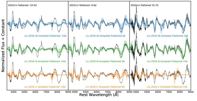
Figure 15: Observed spectra of SN 2022crv compared to the mean spectra (the solid lines) and the standard deviations (the shaded regions) of SN IIb, Ib and Ic from Liu et al. (2016). The observed spectra have been flattened using SNID.

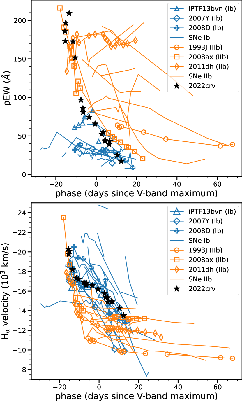
Figure 16: Upper: the pEW evolution of the 6200Å feature of SN 2022crv compared to other SESNe. The 6200 Å feature in SN 2022crv shows a large pEW at the beginning, similar to other SNe IIb. Then it quickly decreases until the 6200 Å feature disappears at around 15 days after $V_{\rm max}$. Bottom: Velocity evolution of the 6200 Å feature in SN 2022crv assuming it is from $\rm H{\alpha}$. The velocity of the 6200 Å feature in SN 2022crv is generally larger than those in SNe IIb but similar to those in SNe Ib.

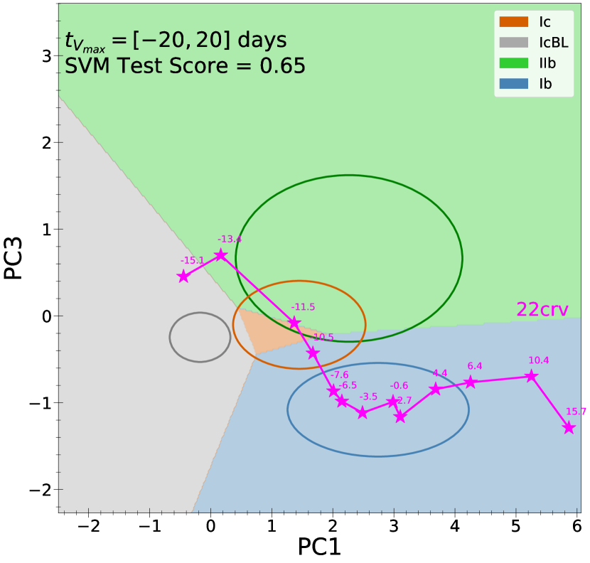
Figure 17: A SVM time dependent spectral classification of SN 2022crv (Williamson & Modjaz 2023, in prep) based on the methods presented in Williamson et al. (2019). SN 2022crv is classified as a Type IIb SN before around -10 days from V-band maximum. After that, SN 2022crv is more similar to a Type Ib. The trajectory in principal component analysis (PCA) phase space as 2022crv evolves (magenta) clearly shows the type transition occurring in the spectra.

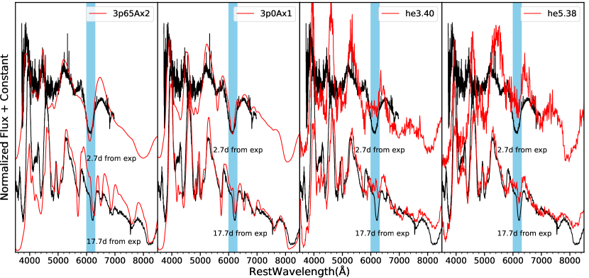
Figure 18: Comparison of the optical spectra of SN 2022crv 2.7d and 17.7d from the explosion with models from Dessart et al. (2016) and Woosley et al. (2021) at similar epochs. The 6200 Å feature is marked by the blue shading. The He3.40 and the He5.38 models are hydrogen-free models, while the 3p65Ax2 and the 3p0Ax1 models retain a small amount of hydrogen.

6 Discussion

6.1 Classification

Although there are clear definitions for each subtype of SESNe, actual classification for individual objects can be nontrivial. This is because the classification for some objects can be time dependent (e.g., Milisavljevic et al., 2013; Folatelli et al., 2014; Williamson et al., 2019; Holmbo et al., 2023). In addition, there is likely a continuum between the subtypes (although see Holmbo et al. 2023). For instance, it has been suggested there is likely a gradual transition from Type IIb to Type Ib depending on the amount of residual hydrogen in the envelope (e.g., Prentice & Mazzali, 2017). Furthermore, hydrogen has been suspected to be present in many Type Ib SNe, suggesting these objects may still maintain low-mass hydrogen envelopes (e.g., Deng et al., 2000; Branch et al., 2002; Elmhamdi et al., 2006; Parrent et al., 2007; James & Baron, 2010). This breaks the Type Ib definition of no hydrogen, and makes the line between Type Ib and Type IIb more vague. In recent years, many efforts have been made to improve the classification system of SESNe (Liu et al., 2016; Prentice & Mazzali, 2017; Williamson et al., 2019; Holmbo et al., 2023). These studies assume there are hydrogen features in both Type Ib and Type IIb, and the difference between them is the evolution and the strength of the $\rm H\alpha$ line. In this section, we will discuss the classification of SN 2022crv and show that this object seems to be an outlier of some classification schemes mentioned above.

SN 2022crv was initially classified as a Type Ib SN (Andrews et al., 2022). However, as we discussed in section 5, a strong absorption line is visible around 6200 Å  during early phases and could be related to $\rm H\alpha$, making the classification of SN 2022crv uncertain. Shortly after the maximum, this line disappears and the spectral evolution of SN 2022crv is almost identical to other SNe Ib. A small notch at around 4595 Å is observed at early phases in SN 2022crv (see Figure 6) and could be due to $\rm H\beta$. To get a better sense of where SN 2022crv stands among SESNe, we compare the observed spectra with the mean spectral templates of SNe IIb, Ib and Ic from Liu et al. (2016) in Figure 15. The observed spectra shown here have been flattened using SNID following the procedure outlined in Blondin & Tonry (2007). At about day $-$10 and day 0, the 6200 Å absorption lines in SN 2022crv are as strong as those in the mean spectra of SNe IIb. However, the 6200 Å absorption line in SN 2022crv is at a higher velocity than those in the mean spectra of SNe IIb, and at a similar velocity to those in the mean spectra of SNe Ib. At about day 15, the spectrum of SN 2022crv is almost identical to the mean spectra of SNe Ib, while the mean spectra of SNe IIb still show a strong 6200 Å absorption line.

If the 6200 Å line is indeed attributed to $\rm H\alpha$, SN 2022crv should be classified as a Type IIb. However, the high-velocity and the rapid disappearance of $\rm H\alpha$ complicates the classification. Liu et al. (2016) found that the $\rm H\alpha$ velocities in SNe Ib are systematically larger than in SNe IIb, and the pEW values in SNe Ib are smaller than in SNe IIb, consistent with the consensus that SNe IIb have more hydrogen in their envelopes. They thus proposed that the pEW can be used to differentiate between SNe Ib and SNe IIb at all epochs. That being said, if an object is classified as a Type Ib/Type IIb using the $\rm H\alpha$ pEW, the classification will not change over time since Type IIb always maintain a larger $\rm H\alpha$ pEW. This result has been further supported by Holmbo et al. (2023) based on the spectroscopic analysis of a large sample of SESNe. In Figure 16, we compare the velocity and pEW evolution of the 6200 Å absorption line in SN 2022crv assuming it is from $\rm H\alpha$ with those of objects presented in Liu et al. (2016). SN 2022crv shows a high pEW at early phases similar to other SNe IIb, followed by a rapid decline, and has a similar pEW value to other SNe Ib about 10 days after the $V$-band maximum. The velocity of SN 2022crv is generally higher than SNe IIb and its evolution is more similar to those of SNe Ib. This pEW transition from SNe IIb to SNe Ib seems to be an outlier of the classification scheme using the pEW of $\rm H{\alpha}$ proposed by Liu et al. (2016).

To quantitatively illustrate the complication of classification, we applied the principal component and SVM classification method described in Williamson et al. (2019). The code has been updated to allow a time-dependent classification of SESNe (Williamson & Modjaz 2023, in prep). The result is shown in Figure 17. Initially, SN 2022crv is located in the Type Ic-BL (broad line) region. This is likely due to the spectrum at day $-$15.1 which is dominated by the strong high-velocity $\rm H{\alpha}$, which can be misidentified as the broad Si II $\lambda$6355 line in SNe Ic-BL. At roughly day $-$13 to day $-$10, SN 2022crv is more similar to SNe IIb. After day $-$10, it is more consistent with SNe Ib.

Prentice & Mazzali (2017) proposed to use the strength and ratio between absorption and emission of $\rm H{\alpha}$ to classify He-rich SNe. They suggested that He-rich SESNe can be split into four groups, IIb, IIb(I), Ib(II) and Ib, from Hydrogen rich to Hydrogen poor. Following the method described in Prentice & Mazzali (2017), the ratio between absorption and emission of $\rm H{\alpha}$ in SN 2022crv before peak is measured to be $\sim$0.3, and the average EW before the maximum is about 73 Å. These values make SN 2022crv marginally fall into the IIb(I) category. The ratio between absorption and emission of $\rm H{\alpha}$ is a good probe of the extent of the hydrogen envelope, and a larger ratio indicates a more extended hydrogen envelope (Prentice & Mazzali, 2017). A classification of IIb(I) implies that the amount of hydrogen in SN 2022crv is larger than normal SNe Ib but smaller than SNe IIb, suggesting SN 2022crv is an intermediate object between these two classes.

In summary, SN 2022crv shares similarities with both Type IIb and Type Ib. The $\rm H{\alpha}$ velocity evolution of SN 2022crv is consistent with those of SNe Ib. The pEW evolution of SN 2022crv gradually transitions from SNe IIb to SNe Ib, a behaviour not observed in the sample studied by Liu et al. (2016). The amount of hydrogen in SN 2022crv is likely between those in SNe Ib and SNe IIb, suggesting SN 2022crv is a representative transitional object on the continuum between SNe IIb and SNe Ib.

6.2 Hydrogen Envelope

Quantifying how much hydrogen is still present in the progenitor right before the explosion is important for understanding the mass loss history and thus the progenitor system. In this section, we will use both a semi-analytic method and hydrodynamic modeling to constrain the mass of hydrogen retained in the progenitor right before the explosion.

The velocity of $\rm H{\alpha}$ in SN 2022crv is generally higher than those of SNe IIb. The higher velocity of $\rm H{\alpha}$ could be a result of higher explosion energy or smaller hydrogen mass. Assuming that the He I line appears when the surrounding hydrogen envelope becomes optically thin and SN expansion is homologous, Marion et al. (2014) proposed a method to roughly estimate the mass of the hydrogen envelope: $M_{\rm H}\propto(v_{\rm H}\times t_{\rm He})^{2}$, where $v_{\rm H}$ is the velocity of the outer edge of the hydrogen envelope and $t_{\rm He}$ is the time when the He line is first observed, and the constant of proportionality is empirically calculated by scaling to a reference supernova. For SN 2022crv, $v_{\rm H}$ is about 30,000 km s^-1. The He line in SN 2022crv can be clearly seen in the first spectrum, so we can limit $t_{\rm He}<$ 2.7d. Using SN 1993J and SN 2011dh as references, we find $\rm M_{H}(2022crv)<0.14\times M_{H}(2011dh)$ and $\rm M_{H}(2022crv)<0.05\times M_{H}(1993J)$. For SN 2011dh and SN 1993J, a recent study by Gilkis & Arcavi (2022) estimated hydrogen masses of $\sim$0.035 $\rm M_{\odot}$ and $\sim$0.1 $\rm M_{\odot}$, respectively. Therefore, the hydrogen envelope mass in SN 2022crv can be constrained to be $\rm M_{H}(2022crv)<5\times 10^{-3}$ $\rm M_{\odot}$. This small hydrogen mass is consistent with the higher velocity and the quick disappearance of the H$\alpha$ in SN 2022crv. However, this seems contrary to the large pEW at early phase.

In order to investigate if a small hydrogen envelope can produce the evolution of the H$\alpha$ line in SN 2022crv, we compare the observed spectra of SN 2022crv with the SESNe models in Dessart et al. (2015, 2016) (3p65Ax2 and 3p0Ax1) and Woosley et al. (2021) (He3.40 and He5.38) (see Figure 18). The He3.40 and the He5.38 model spectra are produced based on models presented in Woosley (2019) and Ertl et al. (2020). These models do not include any hydrogen. The 3p65Ax2 and the 3p0Ax1 model spectra are based on models presented in Yoon et al. (2010). The hydrogen masses in the 3p65Ax2 and 3p0Ax1 models are $4.72\times 10^{-3}$ $\rm M_{\odot}$ and $7.92\times 10^{-4}$ $\rm M_{\odot}$, respectively.

Both the 3p65Ax2 and 3p0Ax1 models nicely reproduce the early-time broad absorption line at 6200 Å and other main features in the observed spectra (Figure 18), while the 3p0Ax1 model gives a better fit. The 6200 Å feature in these two models has been attributed to $\rm H{\alpha}$ at early phase and Si II before the maximum light (Dessart et al., 2015). This is also likely what happened in SN 2022crv. At early time, the broad absorption line at 6200 Å is mainly from hydrogen. As the object evolves, the 6200 Å feature becomes narrower and more dominated by Si II. The 6200 Å feature is missing in the hydrogen-free He3.40 and He5.38 models at 2.7d. At 17.7 d after the explosion, these models show weak absorption lines at around 6200 Å which are identified as Si II in Woosley et al. (2021). We note that the models we use here are not specifically made for SN 2022crv, so the hydrogen mass we get here can be only treated as an order of magnitude estimation. For example, the models from Dessart et al. (2016) have peak luminosities fainter than SN 2022crv, this could be due to the lower explosion energy or lower nickel mass synthesized in the model. Detailed modeling would be required for future studies to better constrain the mass of hydrogen left in the progenitor envelope of SN 2022crv.

The early light curve of SN 2022crv does not show signs of cooling envelope emission, and the nebular spectra also lack hydrogen emission, consistent with the compact progenitor scenario proposed by Chevalier & Soderberg (2010). Given the very low hydrogen mass, the progenitor of SN 2022crv is likely an extreme-version of compact star.

In conclusion, the hydrogen envelope in SN 2022crv is likely on the order of $10^{-3}$ $\rm M_{\odot}$. From the model comparison, we found that the 6200Å line is likely a mixture of $\rm H{\alpha}$ and Si II. At early phases (within 15 days after the explosion), the 6200Å line is likely dominated by hydrogen. After that, the 6200Å is likely mainly due to Si II.

6.3 Explosion Properties

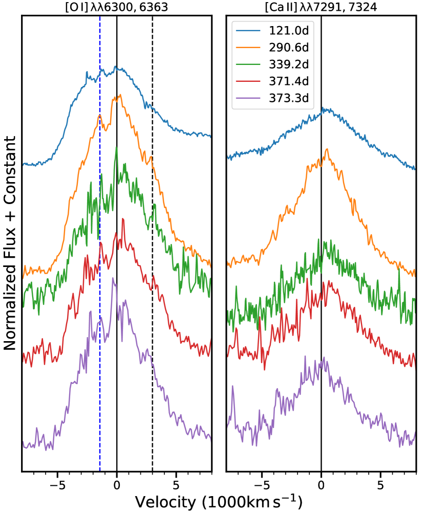
Figure 19: Late-time profile of [O I] $\lambda\lambda$6300, 6364 and [Ca II] $\lambda\lambda$7291, 7323. The phase is measured from the explosion. The zero points for [O I] and [Ca II] are 6300 Å and 7307.5 Å  respectively, and are marked by the solid vertical lines in each panel. The black vertical dashed line in the left panel marks 6364 Å. The blue vertical dashed line marks the blue-shifted peak at around 6270 Å.

6.3.1 Explosion Geometry

At late times, when the SNe ejecta become optically thin, spectra can provide useful information about the inner structure of the SNe. For SESNe, the line profile of [O I] $\lambda\lambda$6300,6364 is often used to study the geometry of the explosion (Mazzali et al., 2005; Maeda et al., 2008; Modjaz et al., 2008; Taubenberger et al., 2009; Milisavljevic et al., 2010; Fang et al., 2022). The [O I] line in SN 2022crv shows an asymmetric profile (see Figure 19), with a prominent peak at around 6300 Å and a blue-shifted peak at around 6270 Å ($-$1430 $\rm km\,s^{-1}$). The separation of the two peaks is 30 Å  smaller than the separation of [O I] $\lambda\lambda$6300,6364 doublet. An asymmetric profile could originate from the oxygen-rich material with a torus-like structure (Mazzali et al., 2005; Maeda et al., 2008; Valenti et al., 2008). However, in this model, the [O I] line would display either a double-peaked profile if viewed from a direction close to the plane of the torus or a single-peaked profile if viewed from a direction perpendicular to the torus. Such a scenario is hard to explain in the case of SN 2022crv due to the lack of a redshifted emission line. If this asymmetric profile is indeed from a torus-like structure, then the emission from the rear side is likely scattered by the ejecta or absorbed by dust (Milisavljevic et al., 2010). For SN 2022crv, a clear sign of CO formation is detected about 100 days after the explosion (Rho et al., in prep), implying dust could form at sufficiently late phases.

Maurer et al. (2010) suggested that the double-peaked profile observed in the [O I] line can be caused by the high-velocity $\rm H{\alpha}$ absorption. Given that a high-velocity feature is detected at early phases for SN 2022crv, this scenario can not be ruled out. If the trough at around 6285 Å is due to $\rm H{\alpha}$ absorption, the corresponding velocity would be $\sim$12,700 $\rm km\,s^{-1}$. There is no clear evidence of $\rm H{\beta}$ found in the nebular spectra of SN 2022crv, likely due to the low signal-to-noise ratio of the blue portion of the spectra. If $\rm H{\alpha}$ is responsible for the asymmetric profile of the [O I] line, the ejecta of SN 2022crv would be almost spherically symmetric.

Table 6: A summary of the nebular spectral models which were compared to SN 2022crv.

Model	$M_{\rm ZAMS}$	$M_{\rm preSN}$	$M_{\rm He}$	$M_{\rm O}$	Reference
	($\rm M_{\odot}$)	($\rm M_{\odot}$)	($\rm M_{\odot}$)	($\rm M_{\odot}$)
Dessart He5.0	20.8	3.81	5.0	0.592	a
Dessart He6.0	23.3	4.44	6.0	0.974	a
Dessart He8.0	27.9	5.63	8.0	1.71	a
Jerkstrand m12C	12	3.12		0.3	b
Jerkstrand m13G	13	3.52		0.52	b
Jerkstrand m17A	17	5.02		1.3	b

6.3.2 Oxygen Mass And Progenitor Mass

Theoretical studies have shown that the initial progenitor mass of a SN strongly correlates with the oxygen mass in the SN ejecta (Woosley & Weaver, 1995; Jerkstrand et al., 2015; Dessart et al., 2021, 2023). The flux of the [O I] $\lambda\lambda$6300, 6364 emission line during the nebular phase has been demonstrated to be a powerful diagnostic tool to constrain the oxygen mass (Uomoto, 1986; Jerkstrand et al., 2012; Dessart et al., 2021). In addition, the line ratio of [O I] $\lambda\lambda$6300, 6364/[Ca II] $\lambda\lambda$7291, 7323 can be an indicator of the progenitor mass of an SESN, since synthesized Ca is not sensitive to the main sequence mass of the progenitor (Nomoto et al., 2006).

Uomoto (1986) showed that the minimal oxygen mass in the SN ejecta can be calculated with:

$$\frac{M_{oxygen}}{\rm M_{\odot}}=10^{8}\times(D/{\rm Mpc})^{2}\times F([OI])\times\exp(2280{\rm K}/T),$$ (1)

where D is the distance of the SN in Mpc, F([O I]) is the flux of the [O I] line in $\rm erg\,s^{-1}\,cm^{-2}$, and $T$ is the temperature of the oxygen-emitting gas in $\rm K$. $T$ can be estimated by using the [O I] $\lambda$5577/[O I] $\lambda\lambda$6300, 6364 flux ratio. However, the [O I] $\lambda$5577 line in SN 2022crv is not clearly detected, indicating a low temperature. The [O I] $\lambda$5577 was also not detected for SN 1990I, and Elmhamdi et al. (2004) put a lower limit on the [O I] $\lambda$5577/[O I] $\lambda\lambda$6300, 6364 flux ratio by using a temperature of 3200 – 3500 K for the line-emitting region of SN 1990I. Sahu et al. (2011) used a temperature of 4000 K for SN 2009jf since the [O I] $\lambda$5577 line was not visible in the nebular spectra of SN 2009jf. For SN 2022crv, we assume the temperature of the line-emitting region is $\sim$3200 K – 4000 K, which results in an oxygen mass of $\sim$0.9 – 3.5 $\rm M_{\odot}$.

In Section 5.2, the [O I]/[Ca II] ratio for SN 2022crv is measured to be $\sim$1.5. Kuncarayakti et al. (2015) measured the [O I]/[Ca II] ratio for a group of CCSNe, and they found that there is a natural spread for SNe Ib/c. This observed spread is likely an indication of two progenitor populations of SESNe: a single massive Wolf-Rayet star and a low-mass star in a binary system. A [O I]/[Ca II] ratio of 1.5 indicates that the progenitor of SN 2022crv is more likely a less massive star. At solar metallicity, the minimum zero-age main sequence (ZAMS) mass ($\rm M_{ZAMS}$) for a single star to lose its hydrogen envelope via stellar winds and become a Wolf-Rayet star is about 25 – 35 $\rm M_{\odot}$ (Crowther, 2007; Sukhbold et al., 2016; Ertl et al., 2020). As we discussed in Section 3.4, the metallicity at the location of SN 2022crv is only slightly larger than solar metallicity. This implies the progenitor was likely in a binary system with a $\rm M_{ZAMS}$ less than about 25 – 35 $\rm M_{\odot}$, and at least a part of the hydrogen envelope was stripped during the binary interaction.

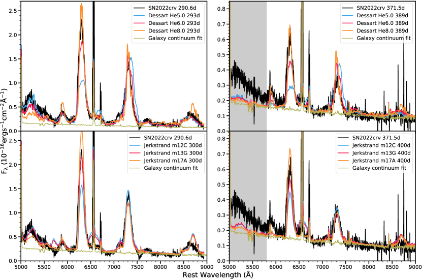
Figure 20: Comparison of the nebular spectra of SN 2022crv at 290.6d and 371.5d post-explosion with models from Jerkstrand et al. (2015) and Dessart et al. (2021). The spectrum is contaminated by the host galaxy, so we fit them with a combination of a star-forming galaxy spectrum and the model SN spectra. For the spectrum at day 371.5, there is a strong background contamination at less than $\sim$5800 Å (marked with grey shading), which makes the observed spectrum clearly depart from the star-forming galaxy spectrum.

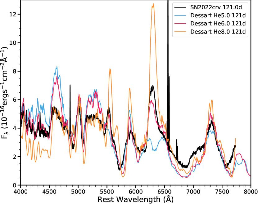
Figure 21: Comparison of the spectrum of SN 2022crv at 121d after the explosion with models from Dessart et al. (2023).

To further constrain the progenitor properties of SN 2022crv, we compare the observed spectrum with theoretical models from Jerkstrand et al. (2015), Dessart et al. (2021), and Dessart et al. (2023). Jerkstrand et al. (2015) took the single-star Type II models from Woosley & Heger (2007) and artificially removed most of the hydrogen envelope, and then produced spectra for SNe IIb. Dessart et al. (2021, 2023) modelled nebular spectra of SNe Ib/c based on models from Woosley (2019) and Ertl et al. (2020), which also include the effects of wind loss from the He star after the H envelope is fully stripped via the binary interaction. Dessart et al. (2023) found that the spectral features of SESNe are mainly dependent on their presupernova masses ($\rm M_{preSN}$) and the oxygen yields, so these models can provide constraints on the oxygen mass and $\rm M_{preSN}$ of SN 2022crv.

The nebular spectra of SN 2022crv at day 290.6 and day 371.5 are likely contaminated by the host background. Therefore, we fit the observed spectrum with a linear combination of the SN spectrum and a star-forming galaxy template spectrum from Kinney et al. (1996) as the first-order approximation of the host background. As the SN gets fainter, this contamination becomes more dominant and harder to remove from the SN spectrum. At day 371.5, the object is highly contaminated by the host background below $\sim$5600 Å. However, we note that this contamination does not affect our estimation on the progenitor properties since we are only interested in the region above $\sim$6000 Å. The comparisons are shown in Figure 20 and 21, while the physical properties of these models are summarized in Table 6.

For the models from Dessart et al. (2021, 2023), we found that the [O I] intensity of SN 2022crv is between those of the He6.0 and He8.0 models. Other features of the observed spectrum, such as Na I $\lambda\lambda$5896,5890, [N II] $\lambda\lambda$ 6548,6583 and [Ca II] $\lambda\lambda$7291,7323, can also be reproduced by these two models. This indicates that the mass of oxygen in SN 2022crv is about 1.0 – 1.7 $\rm M_{\odot}$, and the $\rm M_{preSN}$ is about 4.5 – 5.6 $\rm M_{\odot}$. The corresponding ZAMS star mass of the He6.0 and He8.0 models are 23.3$\rm M_{\odot}$ and 27.9$\rm M_{\odot}$, respectively. For the models from Jerkstrand et al. (2015), we found that the best-fit models are m13G and m17A, while the [N II] $\lambda\lambda$6548,6583 is stronger in model m13G than in the observed spectrum. This suggests that the oxygen mass produced in SN 2022crv is about 0.5 – 1.3$\rm M_{\odot}$, and the $\rm M_{preSN}$ is about 3.5 – 5 $\rm M_{\odot}$. The corresponding ZAMS star mass of the m13G and the m17A models are 13$\rm M_{\odot}$ and 17$\rm M_{\odot}$, respectively.

The oxygen mass and the $\rm M_{preSN}$ derived from models of Dessart et al. (2021, 2023) are consistent with the oxygen mass derived from the models of Jerkstrand et al. (2015), and they are also consistent with the oxygen mass we estimated using the flux of [O I] emission. Since the models in Woosley (2019) used by Dessart et al. (2021, 2023) employed a more updated progenitor evolution treatment than the models in Woosley & Heger (2007) used by Jerkstrand et al. (2015), we will adopt an oxygen mass of 1.0 – 1.7 $\rm M_{\odot}$ and a $\rm M_{preSN}$ of 4.5 – 5.6 $\rm M_{\odot}$ derived from models of Dessart et al. (2021, 2023).

The models from Dessart et al. (2021, 2023) give a systematically larger $\rm M_{ZAMS}$ than the models from Jerkstrand et al. (2015). This is mainly due to the different mass loss assumptions of these two model sets. The models in Jerkstrand et al. (2015) are Type II models with most of the hydrogen envelope artificially removed. This is equivalent to the progenitor promptly losing most of the hydrogen envelope right before the explosion. Thus, the He core mass would continue to grow until the core collapse due to the hydrogen shell burning. While for the models in Dessart et al. (2021, 2023), the hydrogen envelope of the progenitor star is fully stripped by its binary companion close to the time of central He core ignition when the star first becomes a supergiant. After that, the He star still experiences mass loss due to the winds until core collapse.

Dessart et al. (2021, 2023) found that the oxygen yields of CCSNe is closely related to the $\rm M_{preSN}$ of the He stars or the final He core mass of the single stars. Therefore, in order to synthesize the same amount of oxygen or produce progenitors with the same $\rm M_{preSN}$, the models from Jerkstrand et al. (2015) will always have a smaller $\rm M_{ZAMS}$ than the models from Dessart et al. (2021, 2023) (see also Figure 3 in Dessart et al. 2021).

The progenitor of SN 2022crv still retained a tiny amount of hydrogen right before the explosion. If the progenitor of SN 2022crv was a single star, it likely experienced strong stellar wind mass loss throughout its life. If the progenitor of SN 2022crv was in a binary system, it likely lost a part of its hydrogen envelope close to the time of He core ignition (Woosley, 2019; Ertl et al., 2020). After that, the progenitor experienced continuous mass loss via stellar winds until explosion. In either case, since the hydrogen envelope was never fully stripped, during the mass loss, the hydrogen envelope mass would decrease, but the He core mass would grow continuously due to H shell burning. In order to produce the same amount of oxygen in the core or the same $\rm M_{preSN}$, the progenitor of SN 2022crv must have a $\rm M_{ZAMS}$ smaller than those of the He star models evolved with mass loss used by Dessart et al. (2021, 2023) but larger than the trimmed Type II SNe models used by Jerkstrand et al. (2015). Therefore, the $\rm M_{ZAMS}$ of the progenitor of SN 2022crv has to be less than about 23 – 29 $\rm M_{\odot}$ and larger than about 13 – 17 $\rm M_{\odot}$.

Dessart et al. (2023) explored another set of models without mass loss after the stripping of the hydrogen envelope. These models are probably more suitable to the case of SN 2022crv since they also have intact He cores. However, since these models lose their hydrogen envelope promptly close to the time of He core ignition, they would still overestimate the $\rm M_{ZAMS}$ of the progenitor of SN 2022crv. The largest He star mass explored by this model set is 4.5 $\rm M_{\odot}$, which has a $\rm M_{preSN}$ of 4.5 $\rm M_{\odot}$ and a $\rm M_{ZAMS}$ of 19.5 $\rm M_{\odot}$. The spectral features produced by this model is similar to the He6.0 model evolved with mass loss Dessart et al. (2023), which has a $\rm M_{preSN}$ of 4.44. The zero mass loss models with larger masses are not explored in Dessart et al. (2023), but based on equation 4 in Woosley (2019), we can find that a zero mass loss model that has the same $\rm M_{preSN}$ with the He8.0 model would have a $\rm M_{ZAMS}$ of 22.4 $\rm M_{\odot}$. Therefore, we can further constrain the $\rm M_{ZAMS}$ of the progenitor of SN 2022crv to be less than $\sim$20 – 22 $\rm M_{\odot}$.

Another useful constraint can be placed by using the single star Type II progenitor models that evolved with their hydrogen envelopes. As suggested by Dessart et al. (2021), the final oxygen yields from the single stars would be similar to those from the stripped He stars as long as the He core mass of the former is equal to the $\rm M_{preSN}$ of the latter. A single star has a much denser hydrogen envelope than the progenitor of SN 2022crv, which means its He core mass would grow faster than that of the progenitor of SN 2022crv. Thus, in order to produce the same He core mass, a single star would have a smaller $\rm M_{ZAMS}$ than the progenitor of SN 2022crv. A single star that finally has a He core mass of 4.44 $\rm M_{\odot}$ – 5.63 $\rm M_{\odot}$ would have a $\rm M_{ZAMS}$ of 15.5 $\rm M_{\odot}$ – 18.5 $\rm M_{\odot}$ (Sukhbold et al., 2016). Therefore, we can further constrain the $\rm M_{ZAMS}$ of the progenitor of SN 2022crv to be larger than $\sim$16 $\rm M_{\odot}$ – 19 $\rm M_{\odot}$.

In Section 3.4, we found that the metallicity at the site of SN 2022crv is slightly larger than solar metallicity, implying that the progenitor experienced strong stellar wind mass loss. However, the progenitor of SN 2022crv ($\rm M_{ZAMS}\simeq$16$\rm M_{\odot}$ – 22$\rm M_{\odot}$) is still not massive enough to strip most of its hydrogen envelope by itself (Crowther, 2007; Sukhbold et al., 2016), so the progenitor has to be in a binary system.

Binary interaction usually can not fully strip the hydrogen envelope from the progenitor star (Yoon et al., 2017; Götberg et al., 2017). Whether the progenitor can shed all the rest of hydrogen depends on its wind mass-loss rate (Yoon et al., 2017; Gotberg et al., 2023). Since the progenitor of SN 2022crv likely had a high mass-loss rate, to prevent the hydrogen envelope from being fully stripped by wind and binary interaction, the orbital separation of the binary system needs to be large (Yoon et al., 2017; Götberg et al., 2017; Gotberg et al., 2023). Yoon et al. (2017) studied a grid of Type Ib/IIb models in binary systems, and they found that at metallicity Z = 0.02, assuming a mass ratio of $q$ = 0.9, an orbital period of above $2000$ days (or an initial orbital separation larger than $\sim$2200 $\rm R_{\odot}$) is required for a progenitor with $\rm M_{ZAMS}$ = 18 $\rm M_{\odot}$ in a binary system in order to have some remaining hydrogen envelope left. While for a progenitor with $\rm M_{ZAMS}$ = 16 $\rm M_{\odot}$, the orbital period would be larger than $\sim 1700$ days, which is equivalent to an initial orbital separation of $\sim$1900 $\rm R_{\odot}$. If the initial orbital separation is on the order of $\sim$100 $\rm R_{\odot}$, the progenitor would lose all the hydrogen envelope with such a high metallicity. Therefore, the progenitor of SN 2022crv was likely in a binary system with an initial orbital separation larger than $\sim$1000 $\rm R_{\odot}$.

In conclusion, based on the flux of the [O I] emission line, we found an oxygen mass of 0.9 – 3.6$\rm M_{\odot}$. The [O I]/[Ca II] ratio implies the progenitor of SN 2022crv has a $\rm M_{ZAMS}$ less than about 25 – 35 $\rm M_{\odot}$, which implies the envelope of the progenitor was stripped in a binary system via interaction. By comparing with hydrodynamic models, we found that the oxygen synthesized in the progenitor is about 1.0 – 1.7 $\rm M_{\odot}$, and the progenitor is likely a He star with a final mass of $\sim$4.5 – 5.6 $\rm M_{\odot}$ that has evolved from a 16 – 22$\rm M_{\odot}$ ZAMS star. Given the high metallicity at the SN site and the very low-mass hydrogen envelope, the progenitor of SN 2022crv is likely in a binary system with a large initial orbital separation.

6.3.3 $\rm{}^{56}Ni$ Model Fit

In order to estimate the physical parameters of the object, we applied a simple analytical model to the bolometric light curve of SN 2022crv obtained in section 4.2. The analytical model was proposed for Type Ia SNe (Arnett, 1982; Sutherland & Wheeler, 1984; Cappellaro et al., 1997), and can also be used for SESNe (Clocchiatti & Wheeler, 1997; Valenti et al., 2008, 2011; Lyman et al., 2016). For initially pure $\rm{}^{56}Ni$, the energy production rate of the nickel and cobalt decay can be expressed as (Nadyozhin, 1994):

$$P_{\text{Ni}}(t)=\frac{M_{\text{Ni,0}}}{56m_{u}}\frac{Q_{\text{Ni}}}{~{}}{\tau_{\text{Ni}}}~{}e^{-t/\tau_{\text{Ni}}}=M_{\text{Ni,0}}~{}\epsilon_{\text{Ni}}~{}e^{-t/\tau_{\text{Ni}}}$$ (2)

$$P_{\text{Co}}(t) =\frac{M_{\text{Ni,0}}}{56m_{u}}~{}\frac{Q_{\text{Co}}}{\tau_{\text{Co}}-\tau_{\text{Ni}}}(e^{-t/\tau_{\text{Co}}}-e^{-t/\tau_{\text{Ni}}})$$

$$=M_{\text{Ni,0}}~{}\epsilon_{\text{Co}}~{}(e^{-t/\tau_{\text{Co}}}-e^{-t/\tau_{\text{Ni}}}),$$ (3)

where $Q_{\rm Ni}=1.75$ MeV is the energy released per ⁵⁶Ni decay via gamma-ray photons, $Q_{\rm Co}=3.61$ MeV is the average energy released per ⁵⁶Co decay via gamma-ray photons (assuming all the positrons produced in ⁵⁶Co are annihilated), $\tau_{\rm Ni}=8.8$ days is the lifetime of ⁵⁶Ni, $\tau_{\rm Co}=111.3$ days is the lifetime of ⁵⁶Co, $\rm m_{u}$ = 1.66$\times 10^{-24}$ g is the atomic mass, $\rm\epsilon_{Ni}=3.97\times 10^{10}~{}erg\,s^{-1}\,g^{-1}$ and $\rm\epsilon_{Co}=7.03\times 10^{9}~{}erg\,s^{-1}\,g^{-1}$. The exact ⁵⁶Ni and ⁵⁶Co decay data presented in Nadyozhin (1994) have been used for calculations.

Following Valenti et al. (2008), we divided the light curve into photospheric phase and nebular phase. Based on the Arnett model (Arnett, 1982), the bolometric light curve in the photospheric phase can be written as (Valenti et al., 2008):

$$L_{\rm bol,phot}(t)=~{} M_{\rm Ni,0}~{}e^{-x^{2}}$$

$$\times[(\epsilon_{\rm Ni}-\epsilon_{\rm Co})\int^{x}_{0}A(z)\Gamma(z)dz$$

$$~{}~{}~{}~{}~{}+\epsilon_{\rm Co}\int^{x}_{0}B(z)\Gamma(z)dz],$$ (4)

where $A(z)=2ze^{-2zy+z^{2}}$ and $B(z)=2ze^{-2zy+2zs+z^{2}}$, with $x=\frac{t}{\tau_{m}}$, $y=\frac{\tau_{\rm Co}}{2\tau_{\rm Ni}}$ and $s=\frac{\tau_{m}(\tau_{\rm Co}-\tau_{\rm Ni})}{2\tau_{\rm Co}\tau_{\rm Ni}}$. $\Gamma(z)=1-e^{-A(z\tau_{m})^{-2}}$ is the gamma-ray leakage term, with $A=\frac{3\kappa_{\gamma}M_{ej}}{4\pi v^{2}}$. $\tau_{m}$ is the effective time scale of the light curve:

$$\tau_{m}=\frac{\kappa_{opt}}{\beta c}^{1/2}(\frac{6M_{ej}^{3}}{5E_{k}})^{1/4}$$ (5)

, where $M_{\rm ej}$ is the SN ejecta mass, $E_{k}$ is the kinetic energy of the ejecta, $c$ is the speed of light. We have assumed the optical opacity $\kappa_{opt}$ = 0.07 $\rm cm^{2}\,g^{-1}$ is a constant and $\beta$ = 13.8 is an integration constant.

We note that the gamma-ray leakage term $\Gamma$ we use in Equation 6.3.3 is slightly different from what some studies have used in the literature (i.e., Chatzopoulos et al. 2012). Specifically, the gamma-ray leakage term here is a function of time, so it should be included within the integral. In Valenti et al. (2008), although not explicitly mentioned in the paper, the gamma-ray leakage term was actually within the integral when calculating the model light curves, which is the same way we do it here.

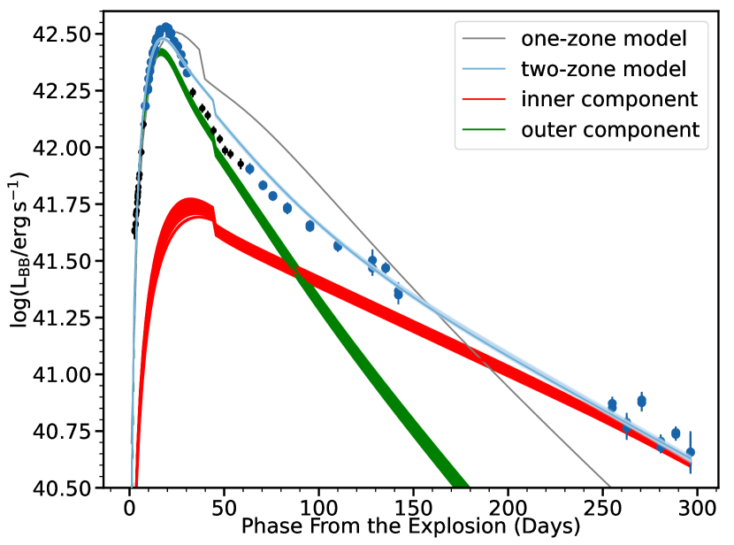
Figure 22: Arnett model fit of the bolometric light curve. The fit is done with a MCMC routine. The best fitting results are represented by the one hundred randomly chosen models draw from the MCMC chain. The blue lines are the two-component fit and the grey lines are the one-component fit. The red lines and the green lines are the contributions from the inner region and the outer region, respectively. Only the blue points are used for the fit. The phase is shown with respect to the explosion epoch.

During the nebular phase, the light curve is powered by the energy deposition produced by the radioactive decay of $\rm{{}^{56}Ni\rightarrow{}^{56}Co\rightarrow{}^{56}Fe}$. Thus, the nebular light curve can be obtained from equation 2 and 6.3.3 by adding the incomplete trapping term of $\gamma$-rays:

$$L_{\rm bol,neb}= ~{}M_{\rm Ni,0}~{}[\epsilon_{\rm Ni}~{}e^{-t/\tau_{Ni}}$$

$$+\epsilon_{\rm Co}~{}(e^{-t/\tau_{\rm Co}}-e^{-t/\tau_{\rm Ni}})](1-e^{-\tau_{\gamma}(t)})$$

$$+0.032\,M_{\rm Ni,0}~{}\epsilon_{\rm Co}~{}(e^{-t/\tau_{\rm Co}}-e^{-t/\tau_{\rm Ni}})$$ (6)

where $\tau_{\gamma}=\frac{3\kappa_{\gamma}M_{ej}}{4\pi v^{2}}$ is the optical depth to $\gamma$-rays (Chatzopoulos et al., 2009, 2012). The last term takes the kinetic energy of the positrons produced by $\rm{}^{56}Co$ decay into account.

The fit has been done with a MCMC method. The free parameters are $t_{0}$, $M_{\rm ej}$ and $M_{\rm Ni,0}$ with uniform priors, where $t_{0}$ is the explosion epoch. The upper and lower bounds of $t_{0}$ are set to be the first detection and the last non-detection, respectively. The fitting range has been chosen to be from -10 to 15 days from mamximum and 60 days post maximum following Valenti et al. (2008) and Lyman et al. (2016). The best-fitting parameters are constrained to be $M_{\rm Ni,0}=0.20^{+0.03}_{-0.02}$ $\rm M_{\odot}$, $M_{\rm ej}=4.90^{+0.04}_{-0.04}$ $\rm M_{\odot}$, $E_{\rm kin}$=2.46${}^{+0.02}_{-0.03}$$\times 10^{51}$ erg. The best-fitting model is shown in Figure 22 (black line).

The model we use here cannot simultaneously reproduce the photospheric and nebular phase of the light curve of SN 2022crv. If we fit these two phases separately, the nickel mass derived from the photospheric phase will be larger than the nickel mass derived from the nebular phase. The ejecta mass derived from the photospheric phase is too small, resulting in a low gamma-ray trapping rate at late phases, leading to a too steep tail. This contradiction can be easily solved if a two-zone model is considered, with one of which dominating the photospheric phase and another one contributing to the nebular phase (Valenti et al., 2008). In the model we adopted above, the nickel is assumed to be concentrated in the center of the progenitor. In order to explain the observational properties of SESNe, nickel needs to be mixed in the ejecta to some extent (Woosley & Eastman, 1997; Dessart et al., 2012; Bersten et al., 2013; Dessart et al., 2015, 2016; Yoon et al., 2019). Therefore, we adopted the two-zone model initially proposed in Maeda et al. (2003) that has been used for some SESNe (Valenti et al., 2008, 2011; Cano et al., 2014). However, we note that since dust likely started to form at late phases in SN 2022crv (Rho et al., in prep), the dust attenuation could also contribute to this contradiction.

In this model, the ejecta of the SN is divided into two separate zones: a high density inner region and a low density outer region. The nickel is assumed to be homogeneously distributed in the two regions, respectively. In this two-zone model, the free parameters are $t_{0}$, the total nickel mass $M_{\rm Ni,total}$, the total ejecta mass $M_{\rm ej,total}$, the kinetic energy of the inner region $E_{\rm kin,inner}$, and the mass fraction of the inner region to the whole ejecta $\rm F_{inner}$. The final best fitting parameters are constrained to be $M_{\rm Ni,total}=0.18^{+0.06}_{-0.04}$ $\rm M_{\odot}$, $M_{\rm ej,total}=2.78^{+0.05}_{-0.04}$ $\rm M_{\odot}$, $E_{\rm kin,total}$=1.01${}^{+0.02}_{-0.02}\times 10^{51}$erg, $\rm F_{inner}$=0.28${}^{+0.01}_{-0.01}$. The two-component model does give a better fit and the best-fitting model is shown in Figure 22.

Lyman et al. (2016) analysed a group of bolometric light curves of SESNe by fitting the Arnett model. They found that the average explosion parameters for SNe IIb are $M_{\rm Ni}=0.11(0.04)$ $\rm M_{\odot}$, $M_{\rm ej}=2.2(0.8)$ $\rm M_{\odot}$and $E_{\rm kin}$ = 1.0(0.6)$\times 10^{51}$erg. For SNe Ib, these values are $M_{\rm Ni}=0.17(0.16)$ $\rm M_{\odot}$, $M_{\rm ej}=2.6(1.1)$ $\rm M_{\odot}$and $E_{\rm kin}$ = 1.6(0.9)$\times 10^{51}$erg. Similar values have also been found for SESNe in more recent studies (e.g., Taddia et al., 2018). The parameters we derived for SN 2022crv are more similar to those of SNe Ib; but considering the uncertainties, they are consistent with those of both SNe IIb and Ib.

6.3.4 $\rm{}^{56}Ni$ + Magnetar fit

Magnetars are thought to be a possible energy source for SESNe (Maeda et al., 2007; Kasen & Bildsten, 2010). We use a hybrid model in which the object is powered by both $\rm{}^{56}Ni$ decay and magnetar spin down. The luminosity of a SN powered by a central magnetar can be written as (Wang et al., 2015):

$$L_{\rm bol,mag}=e^{-x^{2}}\times\frac{E_{NS}}{\tau_{NS}}\times\int^{x}_{0}C(z)dz$$ (7)

where $C(z)=2ze^{z^{2}}/(1+z\frac{\tau_{m}}{\tau_{NS}})^{2}(1-e^{-A(z\tau_{m})^{-2}})$, with $A=\frac{3\kappa_{\gamma}M_{ej}}{4\pi v^{2}}$.

$$E_{NS}=2\times 10^{52}\frac{M_{NS}}{1.4M_{\odot}}\left(\frac{P_{0}}{1~{}\rm ms}\right)^{-2}\left(\frac{R_{NS}}{10~{}\rm km}\right)^{2}~{}\rm erg$$ (8)

$$\tau_{NS}=1.3\left(\frac{B}{10^{14}~{}\rm G}\right)^{-2}\left(\frac{P_{0}}{10~{}\rm ms}\right)^{2}$$ (9)

are the rotational energy and the spin-down timescale of the magnetar, respectively.

We found that the best-fitting model is dominated by the magnetar, and only a small amount of nickel is present in the ejecta. However, for SESNe, a certain amount of nickel should be in the ejecta and power the early part of the light curve (e.g., Woosley, 2019; Woosley et al., 2021). Therefore, a magnetar dominated model is likely not suitable in the case of SN 2022crv.

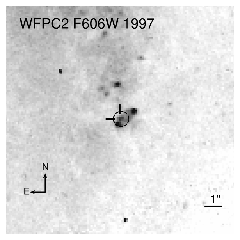
Figure 23: A portion of the HST WFPC2 F606W image mosaic from March 1997, with the location of the SN site indicated by a dashed circle (with radius corresponding to the $3\sigma$ uncertainty in the astrometric registration using a LBT $r$-band image of the SN from March 2022). A stellar-like object with $M_{\rm F606W}\approx-8.2$ mag is indicated by the black tick markers. We tentatively identify this object as the progenitor candidate. North is up, and east is to the left.

6.3.5 Search for a Progenitor Candidate

A pre-explosion image obtained with the Hubble Space Telescope (HST) Wide Field Planetary Camera (WFPC2) in band F606W (PI Stiavelli, SNAP-6359) on 1997 March 27, serendipitously contained the site of SN 2022crv, was identified in the Mikulski Archive for Space Telescope (MAST). We employed a 60-s $r$-band MODS acquisition image of the SN obtained with the LBT on 2022 March 10 to isolate the SN position in the HST image mosaic. We were able to identify 17 stars in common between the two image datasets and, using Photutils centroiding and the PyRAF tasks geomap and geotran, we were able to locate the position with a $1\sigma$ astrometric uncertainty of 1.4 WFPC2 pixels ($0{\farcs}14$) (see Figure 23). The SN site appears to be in a luminous complex of stars or star clusters. We subsequently ran Dolphot (Dolphin, 2016) with PSF fitting photometry on the individual WFPC2 frames and found an object, indicated to be stellar by the routine, with brightness $m_{\rm F606W}=24.07\pm 0.05$ mag. Corrected by our assumed distance and extinction to SN 2022crv, this corresponds to an absolute brightness of $M_{\rm F606W}\approx-8.2$ mag. We tentatively identify this object as the progenitor candidate, although some caution should be applied, given the comparatively low HST resolution with WFPC2. Additionally, with only the single HST band, we have no knowledge of the object’s color. Nevertheless, if we compare its inferred luminosity to, e.g., the progenitor of SN 2011dh, for which Maund et al. (2011) found $M_{\rm F555W}\approx-7.5$ mag (at the assumed distance to M51 of 7.1 Mpc; adjusted to the recent Cepheid distance from Csörnyei et al. 2023, this is $\approx-7.6$ mag) and Van Dyk et al. (2011) estimated as $M_{V}^{0}\approx-7.7$ mag (at an assumed 7.6 Mpc), this progenitor candidate for SN 2022crv appears to be plausible, albeit somewhat more luminous than the SN 2011dh progenitor. We note, however, that, e.g., Eldridge et al. (2015) found that the absolute brightness of the iPTF13bvn progenitor was at most $M_{\rm F555W}\approx-6.5$ mag, so the progenitor candidate for SN 2022crv is significantly more luminous than that. Whether this object is truly the SN progenitor will require confirmation, with follow-up HST observations when the SN has faded significantly (well below mag 24 in F606W).

7 Summary

We present optical and NIR observations of SN 2022crv. In general, the optical photometric and spectroscopic evolution of SN 2022crv resembles those of both SNe IIb and Ib. The object showed conspicuous high-velocity H lines at early phase around 6200 Å, which rapidly disappeared shortly after maximum. The 6200 Å line in SN 2022crv is likely due to H$\alpha$ at early phases and is dominated by Si II $\lambda$6355 after the maximum. The evolution of the H$\alpha$ line pEW in SN 2022crv is similar to those of SNe IIb at early phases, but falls into the Type Ib category shortly after maximum. In addition, we applied a SVM classification method to the spectra ranging from $-$15 days to 15 days relative to the maximum, which classifies SN 2022crv as a Type IIb before $-$10 days and a Type Ib afterwards. This makes SN 2022crv a transitional object on the continuum between Type Ib SNe and Type IIb SNe, and suggests that there is a continuum between these two SN subtypes.

We found that a hydrogen envelope mass of $\sim$10^-3 $\rm M_{\odot}$ in the progenitor can reproduce the behaviours of the H lines in SN 2022crv, and the progenitor is constrained to be a He star with a final mass of $\sim$4.5 – 5.6 $\rm M_{\odot}$ evolving from a $\sim$16 – 22 $\rm M_{\odot}$ ZAMS star in a binary system. The metallicity at the SN site is measured to be slightly higher than the solar metallicity, so the progenitor likely experienced a strong stellar wind mass loss. In this case, an initial orbital separation of the binary system larger than $\sim$1000 $\rm R_{\odot}$ is needed in order to retain a small amount of the hydrogen envelope. We found that the bolometric light curve of SN 2022crv can be best fitted by a model with a nickel mass of $0.18^{+0.06}_{-0.04}$ $\rm M_{\odot}$, $M_{\rm ej}$ of $2.78^{+0.05}_{-0.04}$ $\rm M_{\odot}$, and $E_{\rm kin}$ of 1.01${}^{+0.02}_{-0.02}\times 10^{51}$ erg.

The NIR spectroscopic evolution is generally similar to those of other SNe IIb/Ib. However, an extra absorption feature is observed in the NIR spectra, near the blue side of the He I $\lambda$1.083 $\mu$m line, referred to as feature A in this paper. To the best of our knowledge, feature A has never been observed in other SNe IIb/Ib. We found that this line is most likely from Sr II $\lambda$1.0327 $\mu$m, but we couldn’t safely exclude Fe I $\lambda$1.05 $\mu$m and S I $\lambda$1.0457 $\mu$m. Future detailed modelling is required to further investigate the origin of feature A.

The peculiar features observed in the optical and NIR spectra of SN 2022crv illustrates that SESNe still have many unsolved mysteries. This emphasizes the importance of obtaining NIR spectra and the early discovery of SESNe. As the number of SESNe characterized with detailed datasets increases, the gap between SNe IIb and SNe Ib could be filled, giving us a comprehensive picture of the evolutionary channel and history of the SESNe progenitors.

Appendix A Photometric Data Reduction

The photometric data from the Las Cumbres Observatory were reduced using the PyRAF-based photometric reduction pipeline LCOGTSNPIPE (Valenti et al., 2016). This pipeline uses a low-order polynomial fit to remove the background and calculates instrumental magnitudes using a standard point-spread function (PSF) fitting technique. Apparent magnitudes were calibrated using the APASS ($g,r,i$) and Landolt ($U,B,V$) catalogs.

Unfiltered ($Open$) DLT40 images were processed with a PyRAF-based pipeline. Background contamination was removed by subtracting a reference image, and the aperture photometry was extracted from the subtracted images. The final photometry is calibrated to the $r$ band using the APASS catalog.

The ATLAS survey is carried out primarily in two filters, cyan and orange, roughly equivalent to Pan-STARRS filters g+r and r+i, respectively. A quad of 4 x 30 second exposures are typically obtained for each field over a 1 hour window. The images are processed and difference imaging is performed in real-time to enable rapid discovery of transients in the data stream (Smith et al., 2020). We obtained the forced photometry at the supernova position from the ATLAS forced photometry server (Shingles et al., 2021). We stacked the individual flux measurements for each nightly quad into a single measurement in order to improve signal to noise, and to obtain deeper upper limits for the pre-discovery non-detections.

The images obtained with KAIT and Nickel at Lick Observatory were reduced using a custom pipeline detailed in Stahl et al. (2019). Point-spread function photometry was obtained using DAOPHOT (Stetson, 1987) from the IDL Astronomy User’s Library. Several nearby stars were chosen from the Pan-STARRS1 catalog for calibration. Their magnitudes were first transformed into Landolt magnitudes using the empirical prescription presented by Tonry et al. (2012), then transformed to the KAIT/Nickel natural system. The final result were transformed to the standard system using local calibrators and color terms for KAIT4 and Nickel2 (Stahl et al., 2019).

Swift images were reduced using the High-Energy Astrophysics software (HEA-Soft). The background is measured from a region away from any stars. Zero-points were chosen from Breeveld et al. (2011) with time-dependent sensitivity corrections updated in 2020.

Appendix B Spectroscopic Data Reduction

FLOYDS spectra were reduced following standard procedures using the FLOYDS pipeline (Valenti et al., 2014).

The IMACS Baade spectra were reduced using standard methods and IRAF routines , as described in Hamuy et al. (2006).

The UH88 data were obtained with SNIFS and reduced using the method outlined in Tucker et al. (2022).

The SALT spectra were reduced using a custom longslit pipeline based on the PySALT package (Crawford et al., 2010).

The spectrum taken with the Gemini Multi-Object Spectrographs (GMOS; Hook et al., 2004; Gimeno et al., 2016) as part of our program GN-22A-Q-135 used the B600 grating and a 1.$\arcsec$5 slit. Data were reduced using the DRAGONS (Data Reduction for Astronomy from Gemini Observatory North and South) reduction package (Labrie et al., 2019), using the recipe for GMOS long-slit reductions. This includes bias correction, flatfielding, wavelength calibration, and flux calibration.

The spectrum obtained with the Low Dispersion Survey Spectrograph 3 (LDSS-3) was reduced using iraf including bias subtraction, flat fielding, cosmic ray rejection, local sky subtraction and extraction of one-dimensional spectra. The slit was aligned along the parallactic angle to minimize differential light losses, and flux calibration was done using a spectrophotometric standard taken that night at similar airmass.

The Keck NIRES data were reduced following standard procedures described in the IDL package Spextools version 5.0.2 for NIRES (Cushing et al., 2004). The extracted 1D spectrum was flux calibrated and also corrected for telluric features with Xtellcorr (Vacca et al., 2003) version 5.0.2 for NIRES, making use of an A0V standard star close in time and at similar airmass to the science target.

The two spectra taken with the Kast double spectrograph (Miller & Stone, 1994) mounted on the Shane 3 m telescope at Lick Observatory utilized the 2” slit, 600/4310 grism, and 300/7500 grating. This instrument configuration has a combined wavelength range of   3500-10,500 A, and a spectral resolving power of R $\approx$ 800. To minimize slit losses caused by atmospheric dispersion (Filippenko, 1982), the slit was oriented at or near the parallactic angle. The data were reduced following standard techniques for CCD processing and spectrum extraction (Silverman et al., 2012) utilizing IRAF (Tody, 1986) routines and custom Python and IDL codes. Low-order polynomial fits to comparison-lamp spectra were used to calibrate the wavelength scale, and small adjustments derived from night-sky lines in the target frames were applied. The spectra were flux calibrated using observations of appropriate spectrophotometric standard stars observed on the same night, at similar airmasses, and with an identical instrument configuration.

The NIR spectrum obtained using the Folded port InfraRed Echellette (FIRE; Simcoe et al., 2013) spectrograph mounted on the 6.5-m Magellan Baade telescope at Las Campanas Observatory, Chile, was taken in the high-throughput prism mode with a 0$\farcs$6 slit. For telluric correction, an A0V star was observed close in time and at similar airmass to the science target. The spectra were reduced using the IDL pipeline firehose (Simcoe et al., 2013). Details of the observation setup and reduction were outlined in Hsiao et al. (2019).

NIR spectra were obtained with the MMT and Magellan Infrared Spectrograph (MMIRS; McLeod et al., 2012) on the 6.5 m MMT Observatory telescope on Mt. Hopkins at the Smithsonian’s Fred Lawrence Whipple Observatory using a 1$\farcs$0 slit in both the zJ and HK (with the high-throughput HK3 filter) spectroscopic modes. The data were reduced using the automated MMIRS pipeline (Chilingarian et al., 2015). Telluric corrections and absolute flux calibrations were performed using observations of the A0V star HD 72033 close in time and at similar airmass to the science target. We employed the method of Vacca et al. (2003) implemented in the IDL tool xtellcor_general developed by Cushing et al. (2004) as part of the Spextool package.

The Keck LRIS spectra were reduced in the standard manner with PypeIt (Prochaska et al., 2020a, 2020, b).

The GTC spectrum was reduced following standard procedures with pyraf routines via the graphical user interface FOSCGUI. The two-dimensional frames were corrected for bias and flat-fielded before the one-dimensional spectra extraction. We wavelength-calibrated the spectra via comparison with arc-lamp spectra and calibrated the flux using spectrophotometric standard stars. These also helped in removing the strongest telluric absorption bands present in the spectrum. Finally, the absolute flux calibration of the spectrum was cross-checked against the broadband photometry.

References

- Aldering et al. (1994) Aldering, G., Humphreys, R. M., & Richmond, M. 1994, AJ, 107, 662, doi: 10.1086/116886
- Allende Prieto et al. (2001) Allende Prieto, C., Lambert, D. L., & Asplund, M. 2001, ApJ, 556, L63, doi: 10.1086/322874
- Allington-Smith et al. (1994) Allington-Smith, J., Breare, M., Ellis, R., et al. 1994, PASP, 106, 983, doi: 10.1086/133471
- Andrews et al. (2022) Andrews, J. E., Lundquist, M., Sand, D. J., et al. 2022, Transient Name Server Classification Report, 2022-454, 1
- Arnett (1982) Arnett, W. D. 1982, ApJ, 253, 785, doi: 10.1086/159681
- Asplund et al. (2009) Asplund, M., Grevesse, N., Sauval, A. J., & Scott, P. 2009, ARA&A, 47, 481, doi: 10.1146/annurev.astro.46.060407.145222
- Astropy Collaboration et al. (2013) Astropy Collaboration, Robitaille, T. P., Tollerud, E. J., et al. 2013, A&A, 558, A33, doi: 10.1051/0004-6361/201322068
- Astropy Collaboration et al. (2018) Astropy Collaboration, Price-Whelan, A. M., Sipőcz, B. M., et al. 2018, AJ, 156, 123, doi: 10.3847/1538-3881/aabc4f
- Becker (2015) Becker, A. 2015, HOTPANTS: High Order Transform of PSF ANd Template Subtraction. http://ascl.net/1504.004
- Bersten et al. (2013) Bersten, M. C., Tanaka, M., Tominaga, N., Benvenuto, O. G., & Nomoto, K. 2013, ApJ, 767, 143, doi: 10.1088/0004-637X/767/2/143
- Bertin et al. (2002) Bertin, E., Mellier, Y., Radovich, M., et al. 2002, in Astronomical Society of the Pacific Conference Series, Vol. 281, Astronomical Data Analysis Software and Systems XI, ed. D. A. Bohlender, D. Durand, & T. H. Handley, 228
- Blondin & Tonry (2007) Blondin, S., & Tonry, J. L. 2007, ApJ, 666, 1024, doi: 10.1086/520494
- Bradley et al. (2022) Bradley, L., Sipőcz, B., Robitaille, T., et al. 2022, astropy/photutils: 1.5.0, 1.5.0, Zenodo, doi: 10.5281/zenodo.6825092
- Branch et al. (2002) Branch, D., Benetti, S., Kasen, D., et al. 2002, ApJ, 566, 1005, doi: 10.1086/338127
- Breeveld et al. (2011) Breeveld, A. A., Landsman, W., Holland, S. T., et al. 2011, in American Institute of Physics Conference Series, Vol. 1358, Gamma Ray Bursts 2010, ed. J. E. McEnery, J. L. Racusin, & N. Gehrels, 373–376, doi: 10.1063/1.3621807
- Brethauer et al. (2022) Brethauer, D., Margutti, R., Milisavljevic, D., et al. 2022, ApJ, 939, 105, doi: 10.3847/1538-4357/ac8b14
- Brown et al. (2013) Brown, T. M., Baliber, N., Bianco, F. B., et al. 2013, PASP, 125, 1031, doi: 10.1086/673168
- Burns et al. (2021) Burns, C., Hsiao, E., Suntzeff, N., et al. 2021, The Astronomer’s Telegram, 14441, 1
- Cano et al. (2014) Cano, Z., Maeda, K., & Schulze, S. 2014, MNRAS, 438, 2924, doi: 10.1093/mnras/stt2400
- Cappellaro et al. (1997) Cappellaro, E., Mazzali, P. A., Benetti, S., et al. 1997, A&A, 328, 203, doi: 10.48550/arXiv.astro-ph/9707016
- Cepa et al. (2000) Cepa, J., Aguiar-Gonzalez, M., Gonzalez-Escalera, V., et al. 2000, in Optical and IR Telescope Instrumentation and Detectors, ed. M. Iye & A. F. M. Moorwood, Vol. 4008, International Society for Optics and Photonics (SPIE), 623 – 631, doi: 10.1117/12.395520
- Chatzopoulos et al. (2009) Chatzopoulos, E., Wheeler, J. C., & Vinko, J. 2009, ApJ, 704, 1251, doi: 10.1088/0004-637X/704/2/1251
- Chatzopoulos et al. (2012) —. 2012, ApJ, 746, 121, doi: 10.1088/0004-637X/746/2/121