Mitigating Over-Smoothing and Over-Squashing using Augmentations of Forman-Ricci Curvature

\nameLukas Fesser \emaillukas_fesser@fas.harvard.edu
\addrHarvard University
\nameMelanie Weber \emailmweber@seas.harvard.edu
\addrHarvard University
Abstract

While Graph Neural Networks (GNNs) have been successfully leveraged for learning on graph-structured data across domains, several potential pitfalls have been described recently. Those include the inability to accurately leverage information encoded in long-range connections (over-squashing), as well as difficulties distinguishing the learned representations of nearby nodes with growing network depth (over-smoothing). An effective way to characterize both effects is discrete curvature: Long-range connections that underlie over-squashing effects have low curvature, whereas edges that contribute to over-smoothing have high curvature. This observation has given rise to rewiring techniques, which add or remove edges to mitigate over-smoothing and over-squashing. Several rewiring approaches utilizing graph characteristics, such as curvature or the spectrum of the graph Laplacian, have been proposed. However, existing methods, especially those based on curvature, often require expensive subroutines and careful hyperparameter tuning, which limits their applicability to large-scale graphs. Here we propose a rewiring technique based on Augmented Forman-Ricci curvature (AFRC), a scalable curvature notation, which can be computed in linear time. We prove that AFRC effectively characterizes over-smoothing and over-squashing effects in message-passing GNNs. We complement our theoretical results with experiments, which demonstrate that the proposed approach achieves state-of-the-art performance while significantly reducing the computational cost in comparison with other methods. Utilizing fundamental properties of discrete curvature, we propose effective heuristics for hyperparameters in curvature-based rewiring, which avoids expensive hyperparameter searches, further improving the scalability of the proposed approach.

1 Introduction

Graph-structured data is ubiquitous in data science and machine learning applications across domains. Message-passing Graph Neural Networks (GNNs) have emerged as a powerful architecture for Deep Learning on graph-structured data, leading to many recent success stories in a wide range of disciplines, including biochemistry (Gligorijević et al., 2021), drug discovery (Zitnik et al., 2018), recommender systems (Wu et al., 2022) and particle physics (Shlomi et al., 2020). However, recent literature has uncovered limitations in the representation power of GNNs (Xu et al., 2018), many of which stem from or are amplified by the inability of message-passing graph neural networks to accurately leverage information encoded in long-range connections (over-squashing (Alon and Yahav, 2021)), as well as difficulties distinguishing the learned representations of nearby nodes with growing network depth (over-smoothing (Li et al., 2018)). As a result, there has been a surge of interest in characterizing over-squashing and over-smoothing mathematically and in developing tools for mitigating both effects.

Among the two, over-squashing has received the widest attention, driven by the importance of leveraging information encoded in long-range connections in both node- and graph-level tasks. Over-smoothing has been observed to impact, in particular, the performance of GNNs on node-level tasks. Characterizations of over-squashing and over-smoothing frequently utilize tools from Discrete Geometry, such as the spectrum of the Graph Laplacian (Banerjee et al., 2022; Karhadkar et al., 2022; Black et al., 2023) or discrete Ricci curvature (Topping et al., 2022; Nguyen et al., 2023). Discrete curvature has been linked previously to graph topology and ”information flow” in graphs, which has given rise to several applications in network analysis and machine learning (Ni et al., 2019; Sia et al., 2019; Weber et al., 2017a; Fesser et al., 2023; Tian et al., 2023). Classical Ricci curvature characterizes local volume growth rates on manifolds (geodesic dispersion); analogous notions in discrete spaces were introduced by Ollivier (Ollivier, 2009), Forman (Forman, 2003) and Maas and Erbar (Erbar and Maas, 2012), among others.

Previous work on characterizing over-squashing and over-smoothing with discrete Ricci curvature has utilized Ollivier’s notion (Nguyen et al., 2023) (short ORC), as well as a variation of Forman’s notion (Topping et al., 2022) (FRC). Utilizing ORC is a natural approach, thanks to fundamental relations to the spectrum of the Graph Laplacian and other fundamental graph characteristics (Jost and Liu, 2014), which are known to characterize information flow on graphs. However, computing ORC requires solving an optimal transport problem for each edge in the graph, making a characterization of over-squashing and over-smoothing effects via ORC prohibitively expensive on large-scale graphs. In contrast, FRC can be computed efficiently even on massive graphs due to its simple combinatorial form. Recent work on augmentations of Forman’s curvature, which incorporate higher-order structural information (e.g., cycles) into the curvature computation, has demonstrated their efficiency in graph-based learning, coming close to the accuracy reached by ORC-based methods at a fraction of the computational cost (Fesser et al., 2023; Tian et al., 2023). In this work, we will demonstrate that augmented Forman curvature (AFRC) allows for an efficient characterization of over-squashing and over-smoothing. We relate both effects to AFRC theoretically, utilizing novel bounds on AFRC.

Besides characterizing over-squashing and over-smoothing, much recent interest has been dedicated to mitigating both effects in GNNs. Graph rewiring, which adds and removes edges to improve the information flow through the network, has emerged as a promising tool for improving the quality of the learned node embeddings and their utility in downstream tasks. Building on characterizations of over-squashing (and, to some extend, over-smoothing) discussed above, several rewiring techniques have been proposed (Karhadkar et al., 2022; Banerjee et al., 2022; Topping et al., 2022; Black et al., 2023; Nguyen et al., 2023). Rewiring is integrated into GNN training as a preprocessing step, which alters the graph topology before learning node embeddings. It has been shown to improve accuracy on node- and graph-level tasks, specifically in graphs with long-range connections. Here, we argue that effective rewiring should only add a small computational overhead to merit its integration into GNN training protocols. Hence, the computational complexity of the corresponding preprocessing step, in tandem with the potential need for and cost of hyperparameter searches, is an important consideration. We introduce a graph rewiring technique based on augmentations of Forman’s curvature (AFR-$k$), which can be computed in linear time and which comes with an efficiently computable heuristic for automating hyperparameter choices, avoiding the need for costly hyperparameter searches. Through computational experiments, we demonstrate that AFR-$k$ has comparable or superior performance compared to state-of-the-art approaches, while being more computationally efficient.

Approach O-Smo O-Squ Complexity Hyperparams
SDRF (Topping et al., 2022) $\usym{2717}$ $\usym{2713}$ $O(m\;d_{\max}^{2})$ grid-search
RLEF (Banerjee et al., 2022) $\usym{2717}$ $\usym{2713}$ $O\big{(}n^{2}\sqrt{\log(n)}\;d_{\max}\big{)}$ grid-search
FoSR (Karhadkar et al., 2022) $\usym{2717}$ $\usym{2713}$ $O(n^{2})$ grid-search
BORF (Nguyen et al., 2023) $\usym{2713}$ $\usym{2713}$ $O(m\;d_{\max}^{3})$ grid-search
GTR (Black et al., 2023) $\usym{2717}$ $\usym{2713}$ $O\big{(}m\;{\rm poly}\log n+n^{2}{\rm poly}\log n\big{)}$ grid-search
AFR-3 (this paper) $\usym{2713}$ $\usym{2713}$ $O(m\;d_{\max})$ heuristic
Table 1: Comparison of state-of-the art rewiring approaches for mitigating over-squashing (O-Squ) and over-smoothing (O-Smo) regarding complexity and choice of hyperparameters ($n$ denoting the number of vertices, $m$ the number of edges, $d_{\max}$ the maximal node degree).
Related Work.

A growing body of literature considers the representational power of GNNs (Xu et al., 2018; Morris et al., 2019) and related structural effects (Alon and Yahav, 2021; Li et al., 2018; Di Giovanni et al., 2023; Cai and Wang, 2020; Oono and Suzuki, 2020; Rusch et al., 2022). This includes in particular challenges in leveraging information encoded in long-range connections (over-squashing (Alon and Yahav, 2021)), as well as difficulties distinguishing representations of nearby nodes with growing network depth (over-smoothing (Li et al., 2018)). Rewiring has emerged as a popular tool for mitigating over-squashing and over-smoothing. Methods based on the spectrum of the graph Laplacian (Karhadkar et al., 2022), effective resistance (Black et al., 2023), expander graphs (Banerjee et al., 2022; Deac et al., 2022) and discrete curvature (Topping et al., 2022; Nguyen et al., 2023) have been proposed (see Tab. 1). A connection between over-squashing and discrete curvature was first established in (Topping et al., 2022). To the best of our knowledge, augmented Forman curvature has not been considered as a means for studying and mitigating over-squashing and over-smoothing in previous literature. Notably, the balanced Forman curvature studied in (Topping et al., 2022) is distinct from the notion considered in this paper. Forman’s curvature, as well as discrete curvature more generally, has previously been used in graph-based machine learning, including for unsupervised node clustering (community detection) (Ni et al., 2019; Sia et al., 2019; Tian et al., 2023; Fesser et al., 2023), graph coarsening (Weber et al., 2017b) and in representation learning (Lubold et al., 2022; Weber, 2020).

Contributions.

Our main contributions are as follows:

  • We prove that augmentations of Forman’s Ricci curvature (AFRC) allow for an effective characterization of over-smoothing and over-squashing effects in message-passing GNNs.

  • We propose an AFRC-based graph rewiring approach (AFR-$k$, Alg. 1), which is both scalable and performs competitively compared to state-of-the-art rewiring approaches on node- and graph-level tasks. Importantly, AFR-3 can be computed in linear time, allowing for application of the approach to large-scale graphs.

  • We introduce a novel heuristic for choosing how many edges to add (or remove) in curvature-based rewiring techniques grounded in community detection. This heuristic allows for an effective implementation of our proposed approach, avoiding costly hyperparameter searches. Notably, the heuristic applies also to existing curvature-based rewiring approaches and hence may be of independent interest.

2 Background and Notation

2.1 Message-Passing Graph Neural Networks

Many popular architectures for Graph Machine Learning utilize the Message-Passing paradigm (Gori et al., 2005; Hamilton et al., 2017). Message-passing Graph Neural Networks (short GNNs) iteratively compute node representations as a function of the representations of their neighbors with node attributes in the input graph determining the node representation at initialization. We can view each iteration as a GNN layer; the number of iterations performed to compute the final representation can be thought of as the depth of the GNN. Formally, if we let $\mathbf{X}_{u}^{k}$ denote the features of node $u$ at layer $k$, then a general formulation for a message-passing Graph Neural Network is

$$\mathbf{X}_{u}^{k+1}=\phi_{k}\left(\bigoplus_{p\in\tilde{\mathcal{N}}_{u}}\psi_{k}\left(\mathbf{X}_{p}^{k}\right)\right)$$

Here, $\phi_{k}$ denotes an update function, $\bigoplus$ an aggregation function, and $\psi_{k}$ a message function. $\tilde{\mathcal{N}}_{u}=\mathcal{N}_{u}\cup\{u\}$ is the extended neighborhood of $u$. Widely used examples of this general formulation include GCN (Kipf and Welling, 2017), GIN (Xu et al., 2018) and GAT (Veličković et al., 2018).

2.2 Discrete Ricci Curvature on Graphs

Refer to caption
Figure 1: Augmented Forman-Ricci Curvature.

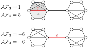
Ricci curvature is a classical tool in Differential Geometry, which establishes a connection between the geometry of the manifold and local volume growth. Discrete notions of curvature have been proposed via curvature analogies, i.e., notions that maintain classical relationships with other geometric characteristics. Forman (Forman, 2003) introduced a notion of curvature on CW complexes, which allows for a discretization of a crucial relationship between Ricci curvature and Laplacians, the Bochner-Weizenböck equation. Here, we utilize an edge-level version of Forman’s curvature, which also allows for evaluating curvature contributions of higher-order structures. Specifically, we consider notions that evaluate higher-order information encoded in cycles of order $\leq k$ (denoted as $\mathcal{AF}_{k}$), focusing on the cases $k=3$ and $k=4$:

$\displaystyle\mathcal{AF}_{3}(u,v)$ $\displaystyle=4-\deg(u)-\deg(v)+3\triangle(u,v)$ (2.1)
$\displaystyle\mathcal{AF}_{4}(u,v)$ $\displaystyle=4-\deg(u)-\deg(v)+3\triangle(u,v)+2\square(u,v)\;,$ (2.2)

where $\triangle(u,v)$ and $\square(u,v)$ denote the number of triangles and quadrangles containing the edge $(u,v)$ (see Fig. 1 for an example). The derivation of those notions follows directly from (Forman, 2003) and can be found, e.g., in (Tian et al., 2023).

2.3 Over-squashing and Over-smoothing

Oversquashing.

It has been observed that bottlenecks in the information flow between distant nodes form as the number of layers in a GNN increases (Alon and Yahav, 2021). The resulting information loss can significantly decrease the effectiveness of message-passing and reduce the utility of the learned node representations in node- and graph-level tasks. This effect is particularly pronounced in long-range connections between distant nodes, such as edges that connect distinct clusters in the graph. Such edges are characterized by low (negative) Ricci curvature in the sense of Ollivier (ORC), giving rise to the curvature-based analysis of over-squashing (Topping et al., 2022; Nguyen et al., 2023). We will show below, that this holds also for AFRC.

Oversmoothing.

At the same time, increasing the number of layers can introduce “shortcuts” between communities, induced by the representations of dissimilar nodes (e.g., nodes belonging to different clusters) becoming indistinguishable under the information flow induced by message-passing. First described by (Li et al., 2018), this effect is known to impact node-level tasks, such as node clustering. It has been previously shown that oversmoothing arises in positively curved regions of the graph in the sense of Ollivier (Nguyen et al., 2023). We will show below, that this holds also for AFRC.

Rewiring.

Graph rewiring describes tools that alter the graph topology by adding or removing edges to improve the information flow in the network. A taxonomy of state-of-the art rewiring techniques and the AFRC-based approach proposed in this paper with respect to the complexity of the resulting preprocessing step and the choice of hyperparameters can be found in Table 1.

3 Characterizing Over-smoothing and Over-squashing with $\mathcal{AF}_{4}$

Before we can relate the augmented Forman-Ricci curvature of an edge to over-smoothing and over-squashing in GNNs, we require upper and lower bounds on $\mathcal{AF}_{3}(u,v)$ and $\mathcal{AF}_{4}(u,v)$. Unlike the Ollivier-Ricci curvature, the augmentations of the Forman-Ricci curvature considered in this paper are not generally bounded independently of the underlying graph. We can prove the following for any (undirected and unweighted) graph $G=(V,E)$:

Theorem 3.1. For $(u,v)\in E$, let $m=\text{deg}(u)\geq\text{deg}(v)=n$. Then for $\mathcal{AF}_{3}$ and $\mathcal{AF}_{4}$, we have

$$\begin{split}4-m-n&\leq\mathcal{AF}_{3}(u,v)\leq n+1\\ 4-m-n&\leq\mathcal{AF}_{4}(u,v)\leq 2mn-3n+3\end{split}$$ (3.1)

Note that these edge-specific bounds can easily be extended to graph-level bounds by noting that $n\leq m\leq\left|V\right|-1$. All other results in this section can be extended to graph-level bounds in a similar fashion. The proof for this result can be found in appendix A.1.1. Our theoretical results and their derivations are largely inspired by Nguyen et al. (2023), although we require several adjustments such as the bounds above, since we are using the AFRC, not the ORC.

From the definition in the last section, it is clear that $\mathcal{AF}_{4}(u,v)$ characterizes how well connected the neighborhoods of $u$ and $v$ are. If many of the nodes in $\mathcal{N}_{u}$ are connected to $v$ or nodes in $\mathcal{N}_{v}$, or vice-versa, then $\mathcal{AF}_{4}$ will be close to its upper bound. Conversely, if $\tilde{\mathcal{N}}_{u}$ and $\tilde{\mathcal{N}}_{v}$ have only minimal connections, then $\mathcal{AF}_{4}(u,v)$ will be close to its lower bound. In the second case, the existing connections will act as bottlenecks and will hinder the message-passing mechanism.

3.1 $\mathcal{AF}_{4}$ and Over-smoothing

Going back to the definition of the message-passing paradigm in the previous section, we note that at the $k$-th layer of a GNN, every node $p$ sends the same message $\psi_{k}\left(\mathbf{X}_{p}^{k}\right)$ to each node $u$ in its neighborhood. The GNN then aggregates these messages to update the features of node $u$. If $\mathcal{AF}_{3}$ or $\mathcal{AF}_{4}$ is very positive, then the neighborhoods of $u$ and $v$ are largely identical, so they receive nearly the same messages, and the difference between their features decreases. The following result makes this intuition for why over-smoothing happens more rigorous. For the proof, see appendix A.1.2.

Theorem 3.2. Consider an updating rule as defined in section 2.1 and suppose that $\mathcal{AF}_{4}(u,v)>0$. For some $k$, assume the update function $\phi_{k}$ is $L$-Lipschitz, $|\mathbf{X}_{p}^{k}|\leq C$ is bounded for all $p\in\mathcal{N}(u)\cup\mathcal{N}(v)$, and the message passing function is bounded, i.e. $|\psi_{k}(\mathbf{x})|\leq M|\mathbf{x}|,\forall\mathbf{x}$. Let $\bigoplus$ be the sum operation. Then there exists a constant $H>0$, depending on $L,M$, and $C$, such that

$$\left|\mathbf{X}_{u}^{k+1}-\mathbf{X}_{v}^{k+1}\right|\leq H(2mn-3n+3-\mathcal{AF}_{4}(u,v))$$ (3.2)

where $m=\text{deg}(u)\geq\text{deg}(v)=n>1$.

We can prove analogous results for $\mathcal{AF}_{3}(u,v)$ when $\bigoplus$ is the mean or the sum operation (A.2.2). Note that Theorem 3.2 applies to most GNN architectures, with the exception of GAT, since GAT uses a learnable weighted mean operation for aggregation. Similar to previous results on the ORC, Theorem 3.2 shows that edges whose augmented Forman-Ricci curvature is close to their upper bound force local node features to become similar. If $\mathcal{AF}_{4}(e)\approx 2mn-3n+3$ for most edges $e$, then we can expect the node features to quickly converge to each other even if the GNN is relatively shallow. For regular graphs, we can extend our analysis and show that the difference between the features of neighboring nodes $u$ and $v$ decays exponentially fast. If in addition, we assume that the diameter of the graph is bounded, then this is true for any pair of nodes $u,v$.

Propositon 3.3. Consider an updating rule as before. Assume the graph is regular. Suppose there exists a constant $\delta$, such that for all edges $(u,v)\in E$, $\mathcal{AF}_{4}(u,v)\geq\delta>0$. For all $k$, assume the update functions $\phi_{k}$ are $L$-Lipschitz, $\bigoplus$ is the mean operation, $|\mathbf{X}_{p}^{0}|\leq C$ is bounded for all $p\in V$, and the message passing functions are bounded linear operators, i.e. $|\psi_{k}(\mathbf{x})|\leq M|\mathbf{x}|,\forall\mathbf{x}$. Then the following inequality holds for $k\geq 1$ and any neighboring vertices $u\sim v$

$$\left|\mathbf{X}_{u}^{k}-\mathbf{X}_{v}^{k}\right|\leq\frac{1}{3}C\left(\frac{3LM(2mn-3n+3-\delta)}{n+1}\right)^{k}$$ (3.3)

If in addition, the diameter of $G$ is bounded, i.e. $d=\max_{u\in V}\max_{v\in V}d(u,v)\leq D$, then for any $u,v\in V$, not necessarily connected, we have

$$\left|\mathbf{X}_{u}^{k}-\mathbf{X}_{v}^{k}\right|\leq\frac{1}{3}DC\left(\frac{3LM(2mn-3n+3-\delta)}{n+1}\right)^{k}$$ (3.4)

For the proof, see appendix A.1.3. The above result gives us the aforementioned exponential decay in differences between node features, since for appropriately chosen $C_{1},C_{2}>0$, we have

$$\sum_{(u,v)\in E}\left|\mathbf{X}_{u}^{k}-\mathbf{X}_{v}^{k}\right|\leq C_{1}e^{-C_{2}k}$$ (3.5)

Even if most real-word graphs possess negatively curved edges, we still expect an abundance of edges whose AFRC is close to its upper bound to lead to over-smoothing in GNNs.

3.2 $\mathcal{AF}_{4}$ and Over-squashing

In this subsection, we relate $\mathcal{AF}_{4}$ to the occurrence of bottlenecks in a graph, which in turn cause the over-squashing phenomenon. Message-passing between neighborhoods requires connections of the form $(p,q)$ for $p\in\tilde{\mathcal{N}}_{u}\setminus\{v\}$ and $q\in\tilde{\mathcal{N}}_{v}\setminus\{u\}$. As the next result shows, the number of these connections can be upper-bounded using $\mathcal{AF}_{4}$. The proof for this can be found in appendix A.1.4.

Proposition 3.4. Let $(u,v)\in E$ and let $S\subset E$ be the set of all $(p,q)$ with $p\in\tilde{N}_{u}\setminus\{v\}$ and $q\in\tilde{N}_{v}\setminus\{u\}$. Then

$$\left|S\right|\leq\frac{\mathcal{AF}_{4}(u,v)+\text{deg}(u)+\text{deg}(v)-4}{2}$$ (3.6)

An immediate consequence of this result is that if $\mathcal{AF}_{4}$ is close to its lower bound $4-\text{deg}(u)-\text{deg}(v)$, then the number of connections between $\tilde{\mathcal{N}}_{u}$ and $\tilde{\mathcal{N}}_{v}$ has to be small. Hence these edges will induce bottlenecks in $G$, which in turns causes over-squashing.

4 $\mathcal{AF}_{3}$- and $\mathcal{AF}_{4}$-based Rewiring

4.1 AFR-3 and AFR-4

Following our theoretical results in the last section, an $\mathcal{AF}_{3}$- or $\mathcal{AF}_{4}$-based rewiring algorithm should remove edges whose curvature is close to the upper bound to avoid over-smoothing, and add additional edges to the neighborhoods of those edges whose curvature is particularly close to the lower bound to mitigate over-squashing. In line with this intuition, we propose AFR-$k$, a novel algorithm for graph rewiring that, like the ORC-based BORF, can address over-smoothing and over-squashing simultaneously, while being significantly cheaper to run.

Algorithm 1 AFR-3
A graph $G(V,E)$, heuristic (Bool), # edges to add $h$, # edges to remove $l$
for $e\in E$ do
     compute $\mathcal{AF}_{3}(e)$
end for
Sort $e\in E$ by $\mathcal{AF}_{3}(e)$
if heuristic == True then
     - Compute lower threshold $\Delta_{L}$. For each $(u,v)\in E$ with $\mathcal{AF}_{3}(u,v)<\Delta_{L}$,
     choose $w\in\mathcal{N}_{u}\setminus\mathcal{N}_{v}$ uniformly at random, add $(w,v)$ to $E$.
     - Compute upper threshold $\Delta_{U}$ and remove all edges $(u,v)$ with $\mathcal{AF}_{3}(u,v)>\Delta_{U}$
else
     - Find $h$ edges with lowest $\mathcal{AF}_{3}$ values, for each of these edges,
     choose $w\in\mathcal{N}_{u}\setminus\mathcal{N}_{v}$ uniformly at random, add $(w,v)$ to $E$.
     - Find $k$ edges with highest $\mathcal{AF}_{3}$ values and remove them from $E$.
end if
return a rewired graph $G^{\prime}=(V,E^{\prime})$ with new edge set $E^{\prime}$.

Assume that we want to add $h$ edges to $E$ to reduce over-squashing, and remove $l$ edges from $E$ to mitigate over-smoothing. Then for AFR-3 without heuristics for edge addition or removal, we first compute $\mathcal{AF}_{3}(e)$ for all $e\in E$. Then, we sort the the edges by curvature from lowest to highest. For each of the $h$ edges with lowest curvature values, we choose $w\in\mathcal{N}_{u}\setminus\mathcal{N}_{v}$ uniformly at random if $\text{deg}(u)\geq\text{deg}(v)$ and add $(w,v)$ to $E$. If no such $w$ exists, we continue on to the next edge. Finally, we remove the $l$ edges with the highest curvature values from $E$. We return the rewired graph $G^{\prime}=(V,E^{\prime})$, where $E^{\prime}$ is the rewired edge set. AFR-4 follows by analogy, only that we use $\mathcal{AF}_{4}$ instead of $\mathcal{AF}_{3}$. While $\mathcal{AF}_{3}$ is cheaper to run than $\mathcal{AF}_{4}$, both are more economical than their ORC-based cousin BORF, which is due to the next result.

Theorem 4.1. Computing the ORC scales as $O\left(\left|E\right|d_{\text{max}}^{3}\right)$, while computing $\mathcal{AF}_{3}$ scales as $O\left(\left|E\right|d_{\text{max}}\right)$, and computing $\mathcal{AF}_{4}$ scales as $O\left(\left|E\right|d_{\text{max}}^{2}\right)$.

Here, $d_{\text{max}}$ is the highest degree of a node in $G$. For the proof, see appendix A.1.5. Note that we could run AFR-3 (AFR-4) as a batch-based algorithm like BORF. For $N$ batches, we would recompute $\mathcal{AF}_{3}$ ($\mathcal{AF}_{4}$) $N$ times, and for each batch we would identify the $k$ edges with highest $\mathcal{AF}_{3}$ ($\mathcal{AF}_{4}$) values and the $h$ edges with lowest $\mathcal{AF}_{3}$ ($\mathcal{AF}_{4}$) values and proceed with them as before. In practice, we find that this rarely improves performance. Results on this are presented in appendix A.7.4.

4.2 Heuristics for adding and removing Edges

A natural question to ask upon seeing the AFR algorithm is how many edges one should add or remove for a given graph $G$. For previous methods such as BORF, answering this question involved costly hyperparameter tuning. In this subsection, we use results from community detection in network science to motivate heuristics to automatically determine $h$ and $k$.

Curvature Thresholds. Suppose we are given a graph $G=(V,E)$ and a partition of the network into communities. As previously mentioned, edges within communities tend to have positive Ollivier-Ricci curvature, while edges between communities tend to have negative curvature values. Theoretical evidence for this observation for graphs with community structure has been given in (Ni et al., 2019; Gosztolai and Arnaudon, 2021; Tian et al., 2023).

Sia et al. (2019) use this observation to propose a community detection algorithm: remove the most negatively curved edge $e$ from $G$, recompute the ORC for all edges sharing a node with $e$ and repeat these two steps until all negatively curved edges have been removed. The connected components in the resulting graph $G^{\prime}$ are the communities. For $\mathcal{AF}_{3}$ or $\mathcal{AF}_{4}$, a natural threshold to distinguish between inter- and intra-community edges is missing, so Fesser et al. (2023) propose to use a Gaussian mixture model with two modes. They fit two normal distributions $\mathcal{N}_{1}(\mu_{1},\sigma_{1})$ and $\mathcal{N}_{2}(\mu_{2},\sigma_{2})$ with $\mu_{1}>\mu_{2}$ to the curvature distribution and then determine the curvature threshold

$$\Delta_{L}=\frac{\sigma_{2}}{\sigma_{1}+\sigma_{2}}\mu_{1}+\frac{\sigma_{1}}{\sigma_{1}+\sigma_{2}}\mu_{2}$$ (4.1)
Refer to caption
Figure 2: Upper and lower thresholds for the Wisconsin dataset ($\mathcal{AF}_{3}$).

Using this as the threshold between inter- and intra-community edges, their $\mathcal{AF}_{3}$-based sequential community detection algorithm achieves competitive performance while being significantly cheaper to run than the ORC-based original. Based on this, we propose the following heuristic to determine the number $h$ of edges to add for AFR.

Heuristic for edge addition. Instead of choosing the number $h$ of edges to add by hand, we calculate the curvature threshold $\Delta_{L}$ as above. We then add a new edge for each edge $e$ with $\mathcal{AF}_{3}(e)<\Delta_{L}$ ($\mathcal{AF}_{4}(e)<\Delta_{L}$) using the same procedure as before.

Heuristic for edge removal. To identify particularly positively curved edges which might lead to over-smoothing, we compute the upper curvature threshold $\Delta_{U}$ as

$$\Delta_{U}=\mu_{1}+\sigma_{1}$$ (4.2)

We remove all edges $e$ with $\mathcal{AF}_{3}(e)>\Delta_{U}$ ($\mathcal{AF}_{4}(e)>\Delta_{U})$, i.e. all edges whose curvature is more than one standard deviation above the mean of the normal distribution with higher curvature values.

5 Experiments

In this section, we experimentally demonstrate the effectiveness and computational efficiency of our proposed AFR rewiring algorithm and of our heuristics for edge addition and removal. We first compare AFR against other rewiring alternatives on a variety of tasks, including node and graph classification, as well as long-range tasks. Details on the rewiring strategies we compare against can be found in appendix A.4. We also show that our heuristics allow AFR to achieve competitive performance on all tasks without costly hyperparameter tuning. Our code will be made publicly available upon publication.

Experimental details. Our experiments are designed as follows: for a given rewiring strategy, we first apply it as a preprocessing step to all graphs in the datasets considered. We then train a GNN on a part of the rewired graphs and evaluate its performance on a withheld set of test graphs. We use a train/val/test split of 50/25/25. As GNN architectures, we consider GCN and GIN. Settings and optimization hyper-parameters are held constant across tasks and baseline models for all rewiring methods, so we can rule out hyper-parameter tuning as a source of performance gain. When not using our heuristics, we obtain the settings for the individual rewiring option via hyperparameter tuning. The only hyperparameter choice which we do not optimize using grid search is $\tau$ in SDRF, which we set to $\infty$, in line with Nguyen et al. (2023). For all rewiring methods and hyperparameter choices, we record the test set accuracy of the settings with the highest validation accuracy. As there is a certain stochasticity involved, especially when training GNNs, we accumulate experimental results across 100 random trials. We report the mean test accuracy, along with the $95\%$ confidence interval. Details on all data sets can be found in appendix A.9.

5.1 Results using hyperparameter search

Tables 2 and 3 present the results of our experiments for node and graph classification with hyperparameter tuning. The exact hyperparameter settings for each dataset can be found in appendix A.3, where we also present additional results using GIN as an architecture (A.7.1). For the experiments with GCNs presented here, AFR-3 and AFR-4 outperform all other rewiring strategies and the no-rewiring baseline on all node classification datasets and on four of our five graph classification datasets. We expect AFR-3, AFR-4, and BORF to attain generally higher accuracies than FoSR and SDRF, because unlike FoSR and SDRF, they can address over-smoothing by removing edges.

GCN
DATA SET AFR-3 AFR-4 BORF SDRF FOSR NONE
CORA $87.5\pm 0.5$ $\mathbf{88.1\pm 0.5}$ $87.9\pm 0.7$ $86.4\pm 2.1$ $86.9\pm 2.0$ $86.6\pm 0.8$
CITESEER $\mathbf{74.4\pm 1.0}$ $73.3\pm 0.6$ $73.4\pm 0.6$ $72.6\pm 2.2$ $73.5\pm 2.0$ $71.7\pm 0.7$
TEXAS $49.7\pm 0.5$ $\mathbf{51.4\pm 0.5}$ $48.9\pm 0.5$ $43.6\pm 1.2$ $46.9\pm 1.2$ $44.1\pm 0.5$
CORNELL $\mathbf{49.7\pm 3.4}$ $48.9\pm 3.3$ $48.1\pm 2.9$ $43.1\pm 1.2$ $43.9\pm 1.1$ $46.8\pm 3.0$
WISCON. $47.3\pm 2.4$ $\mathbf{52.2\pm 2.4}$ $46.5\pm 2.6$ $47.1\pm 1.0$ $48.5\pm 1.0$ $44.6\pm 2.9$
CHAMEL. $62.3\pm 0.9$ $\mathbf{62.5\pm 0.9}$ $61.4\pm 0.9$ $59.5\pm 0.4$ $59.3\pm 1.9$ $59.1\pm 1.4$
COCO $\mathbf{10.1\pm 1.1}$ $9.8\pm 1.1$ $10.1\pm 1.2$ $8.5\pm 1.0$ $9.3\pm 1.4$ $7.8\pm 0.4$
PASCAL $14.3\pm 1.5$ $\mathbf{14.4\pm 1.4}$ $14.1\pm 1.1$ $11.7\pm 0.9$ $13.8\pm 1.3$ $10.4\pm 0.6$
Table 2: Classification accuracies of GCN with AFR-3, AFR-4, BORF, SDRF, FoSR, or no rewiring strategy using best hyperparameters. Highest accuracies on any given dataset are highlighted in bold. We report F1 scores for the LGRB COCO and PASCAL datasets.

Comparing AFR-3 and AFR-4. In section 3, we used $\mathcal{AF}_{4}$ for our theoretical results due to it allowing us to better analyze over-smoothing. However, for many real-world datasets, $\mathcal{AF}_{3}$ and $\mathcal{AF}_{4}$ are highly correlated Fesser et al. (2023). We find that this also holds true for the datasets considered here (see appendix A.9), which might explain why AFR-3, AFR-4, and BORF all achieve comparable accuracies, with AFR-3 and AFR-4 often performing marginally better. This also suggests that characterizing over-smoothing and over-squashing using $\mathcal{AF}_{3}$ or $\mathcal{AF}_{4}$ is sufficient. The computationally more expensive ORC is not needed. In practice, one would always use AFR-3 due to competitive performance and excellent scalability.

GCN
DATA SET AFR-3 AFR-4 BORF SDRF FOSR NONE
MUTAG $69.7\pm 2.1$ $68.7\pm 1.9$ $68.2\pm 2.4$ $65.1\pm 2.2$ $\mathbf{70.0\pm 2.2}$ $62.7\pm 2.1$
ENZYMES $25.9\pm 1.2$ $\mathbf{26.3\pm 1.2}$ $26.0\pm 1.2$ $24.3\pm 1.2$ $24.9\pm 1.1$ $25.4\pm 1.3$
IMDB $\mathbf{50.4\pm 0.9}$ $49.8\pm 1.1$ $48.6\pm 0.9$ $48.6\pm 0.9$ $48.3\pm 0.9$ $48.1\pm 1.0$
PROTEINS $\mathbf{62.7\pm 0.8}$ $61.2\pm 0.9$ $61.5\pm 0.7$ $59.5\pm 0.8$ $59.3\pm 0.9$ $59.6\pm 0.9$
PEPTIDES $\mathbf{44.7\pm 2.8}$ $44.4\pm 2.8$ $43.9\pm 2.6$ $41.8\pm 1.5$ $44.3\pm 2.2$ $40.5\pm 2.1$
Table 3: Classification accuracies of GCN with AFR-3, AFR-4, BORF, SDRF, FoSR, or no rewiring strategy using best hyperparameters. Highest accuracies on any given dataset are highlighted in bold.

5.2 Results using heuristics for edge addition and removal

Using the same datasets as before, we now test our heuristics for replacing hyperparameter tuning. We study the effects of using the thresholds proposed in section 4 on AFR-3, AFR-4, and BORF. Tables 4 and 5 present the accuracies attained by GCN and GIN architectures using our heuristics for finding upper and lower thresholds. Comparing these to the results in Tables 2 and 3, we see that our heuristics outperform hyperparameter tuning on four out of six node classification datasets, and are competitive on the other two. Similarly on the graph classification tasks, where our heuristics achieve superior performance on four out of five tasks.

GCN GIN
DATA SET AFR-3 AFR-4 BORF AFR-3 AFR-4 BORF
CORA $87.8\pm 0.7$ $87.9\pm 0.9$ $87.6\pm 0.7$ $77.9\pm 1.2$ $78.0\pm 1.1$ $78.4\pm 1.1$
CITESEER $74.6\pm 0.7$ $74.7\pm 0.7$ $74.2\pm 0.8$ $65.1\pm 0.7$ $64.7\pm 0.6$ $64.6\pm 0.6$
TEXAS $52.4\pm 3.3$ $48.4\pm 3.2$ $50.5\pm 2.8$ $68.7\pm 3.1$ $63.8\pm 3.8$ $62.3\pm 2.0$
CORNELL $50.5\pm 4.3$ $46.2\pm 2.6$ $44.6\pm 1.9$ $51.9\pm 4.2$ $47.3\pm 2.3$ $48.4\pm 2.5$
WISCON. $52.4\pm 2.6$ $49.0\pm 2.0$ $48.2\pm 3.0$ $58.4\pm 2.9$ $58.7\pm 2.3$ $53.5\pm 2.6$
CHAMEL. $62.2\pm 1.2$ $62.1\pm 1.2$ $61.1\pm 1.4$ $67.1\pm 2.1$ $65.9\pm 2.2$ $66.3\pm 2.2$
COCO $10.3\pm 1.3$ $9.6\pm 1.2$ $10.5\pm 1.2$ $13.1\pm 2.1$ $13.5\pm 2.2$ $13.6\pm 2.2$
PASCAL $14.2\pm 1.5$ $14.3\pm 1.5$ $14.8\pm 1.1$ $16.0\pm 1.7$ $15.8\pm 1.7$ $16.4\pm 1.8$
Table 4: Node classification accuracies of GCN and GIN with AFR-3, AFR-4, and BORF using our heuristics to avoid hyperparameter tuning.

For BORF, we use zero as the lower threshold to identify bottleneck edges. We conduct additional experiments in appendix A.7.7 which show that the lower thresholds which we get from fitting two normal distributions to the ORC distributions are in fact very close to zero on all datasets considered here. Further ablations that study the effects of our two heuristics individually can also be found in appendices A.7.2 and A.7.3.

GCN GIN
DATA SET AFR-3 AFR-4 BORF AFR-3 AFR-4 BORF
MUTAG $71.4\pm 2.2$ $69.9\pm 2.6$ $68.5\pm 1.9$ $70.9\pm 2.7$ $73.4\pm 2.4$ $75.4\pm 2.8$
ENZYMES $26.1\pm 1.0$ $25.5\pm 1.0$ $23.3\pm 1.2$ $37.6\pm 1.2$ $32.1\pm 1.4$ $31.9\pm 1.2$
IMDB $50.1\pm 0.9$ $49.0\pm 0.9$ $49.4\pm 1.0$ $68.9\pm 1.1$ $67.8\pm 1.2$ $67.7\pm 1.5$
PROTEINS $62.2\pm 0.8$ $61.2\pm 0.9$ $61.0\pm 0.9$ $73.0\pm 1.5$ $72.7\pm 1.3$ $72.3\pm 1.2$
PEPTIDES $44.8\pm 2.8$ $43.6\pm 2.5$ $44.3\pm 2.8$ $49.2\pm 1.5$ $50.7\pm 1.6$ $50.1\pm 1.6$
Table 5: Graph classification accuracies of GCN and GIN with AFR-3, AFR-4, and BORF using our heuristics to avoid hyperparameter tuning.

Long-range tasks. We also evaluated AFR-3 and AFR-4 on the Peptides-func graph classification dataset and on the PascalVOC-SP and COCO-SP node classification datasets, which are part of the long-range tasks introduced by Dwivedi et al. (2022). As Table 3 shows, AFR-3 and AFR-4 outperform all other rewiring methods on the graph classification task and significantly improve on the no-rewiring baseline. Our heuristics are also clearly still applicable, as they result in comparable performance (Table 5). Our experiments with long-range node classification yield similar results, as can be seen in Tables 2 and 4. Additional experiments with the LRGB datasets using GIN can be found in A.7.1.

6 Discussion

In this paper we have introduced formal characterizations of over-squashing and over-smoothing effects using augementations of Forman’s Ricci curvature, a simple and scalable notion of discrete curvature. Based on this characterization, we proposed a scalable graph rewiring approach, which exhibits performance comparable or superior to state-of-the-art rewiring approaches on node- and graph-level tasks. We further introduce an effective heuristic for hyperparameter choices in curvature-based graph rewiring, which removes the need to perform expensive hyperparameter searches.

There are several avenues for further investigation. We believe that the complexity of rewiring approaches merits careful consideration and should be evaluated in the context of expected performance gains in applications. This includes in particular the choice of hyperparameters, which for many state-of-the-art rewiring approaches requires expensive grid searches. While we propose an effective heuristic for curvature-based approaches (both existing and proposed herein), we believe that a broader study on transparent hyperparameter choices across rewiring approaches is merited. While performance gains in node- and graph-level tasks resulting from rewiring have been established empirically, a mathematical analysis is still largely lacking and an important direction for future work. Our proposed hyperparameter heuristic is linked to the topology and global geometric properties of the input graph. We believe that similar connections could be established for rewiring approaches that do not rely on curvature. Building on this, a systematic investigation of the suitability of different rewiring and corresponding hyperparameter choices dependent on graph topology would be a valuable direction for further study. Similarly, differences between the effectiveness of rewiring in homophilous vs. heterophilous graphs strike us as an important direction for future work.

7 Limitations

The present paper does not explicitly consider the impact of graph topology on the efficiency of AFR-$k$. Specifically, our proposed heuristic implicitly assumes that the graph has community structure, which is true in many, but not all, applications. Our experiments are restricted to one node- and graph-level task each. While this is in line with experiments presented in related works, a wider range of tasks would give a more complete picture.

References

  • Alon and Yahav (2021) Uri Alon and Eran Yahav. On the bottleneck of graph neural networks and its practical implications. In International Conference on Learning Representations, 2021. URL https://openreview.net/forum?id=i80OPhOCVH2.
  • Banerjee et al. (2022) Pradeep Kr Banerjee, Kedar Karhadkar, Yu Guang Wang, Uri Alon, and Guido Montúfar. Oversquashing in gnns through the lens of information contraction and graph expansion. In 2022 58th Annual Allerton Conference on Communication, Control, and Computing (Allerton), pages 1–8. IEEE, 2022.
  • Black et al. (2023) Mitchell Black, Zhengchao Wan, Amir Nayyeri, and Yusu Wang. Understanding oversquashing in gnns through the lens of effective resistance. In International Conference on Machine Learning, pages 2528–2547. PMLR, 2023.
  • Cai and Wang (2020) Chen Cai and Yusu Wang. A note on over-smoothing for graph neural networks. arXiv preprint arXiv:2006.13318, 2020.
  • Deac et al. (2022) Andreea Deac, Marc Lackenby, and Petar Veličković. Expander graph propagation. In Proceedings of the First Learning on Graphs Conference, 2022.
  • Di Giovanni et al. (2023) Francesco Di Giovanni, Lorenzo Giusti, Federico Barbero, Giulia Luise, Pietro Lio, and Michael M. Bronstein. On over-squashing in message passing neural networks: The impact of width, depth, and topology. In Andreas Krause, Emma Brunskill, Kyunghyun Cho, Barbara Engelhardt, Sivan Sabato, and Jonathan Scarlett, editors, Proceedings of the 40th International Conference on Machine Learning, volume 202 of Proceedings of Machine Learning Research, pages 7865–7885. PMLR, 23–29 Jul 2023.
  • Dwivedi et al. (2022) Vijay Prakash Dwivedi, Ladislav Rampášek, Mikhail Galkin, Ali Parviz, Guy Wolf, Anh Tuan Luu, and Dominique Beaini. Long range graph benchmark. In Thirty-sixth Conference on Neural Information Processing Systems Datasets and Benchmarks Track, 2022. URL https://openreview.net/forum?id=in7XC5RcjEn.
  • Erbar and Maas (2012) M. Erbar and J. Maas. Ricci curvature of finite markov chains via convexity of the entropy. Archive for Rational Mechanics and Analysis, 206:997–1038, 2012.
  • Fesser et al. (2023) Lukas Fesser, Sergio Serrano de Haro Iváñez, Karel Devriendt, Melanie Weber, and Renaud Lambiotte. Augmentations of forman’s ricci curvature and their applications in community detection. arXiv preprint arXiv:2306.06474, 2023.
  • Forman (2003) Robin Forman. Bochner’s Method for Cell Complexes and Combinatorial Ricci Curvature. volume 29, pages 323–374, 2003.
  • Gligorijević et al. (2021) Vladimir Gligorijević, P Douglas Renfrew, Tomasz Kosciolek, Julia Koehler Leman, Daniel Berenberg, Tommi Vatanen, Chris Chandler, Bryn C Taylor, Ian M Fisk, Hera Vlamakis, et al. Structure-based protein function prediction using graph convolutional networks. Nature communications, 12(1):3168, 2021.
  • Gori et al. (2005) Marco Gori, Gabriele Monfardini, and Franco Scarselli. A new model for learning in graph domains. In Proceedings. 2005 IEEE international joint conference on neural networks, volume 2, pages 729–734, 2005.
  • Gosztolai and Arnaudon (2021) Adam Gosztolai and Alexis Arnaudon. Unfolding the multiscale structure of networks with dynamical Ollivier-Ricci curvature. Nature Communications, 12(1), December 2021.
  • Hamilton et al. (2017) William L. Hamilton, Zhitao Ying, and Jure Leskovec. Inductive Representation Learning on Large Graphs. In NIPS, pages 1024–1034, 2017.
  • Jost and Liu (2014) J. Jost and S. Liu. Ollivier’s Ricci curvature, local clustering and curvature-dimension inequalities on graphs. Discrete & Computational Geometry, 51(2):300–322, 2014.
  • Karhadkar et al. (2022) Kedar Karhadkar, Pradeep Kr Banerjee, and Guido Montúfar. Fosr: First-order spectral rewiring for addressing oversquashing in gnns. arXiv preprint arXiv:2210.11790, 2022.
  • Kipf and Welling (2017) Thomas N. Kipf and Max Welling. Semi-Supervised Classification with Graph Convolutional Networks. In ICLR, 2017.
  • Li et al. (2018) Qimai Li, Zhichao Han, and Xiao-Ming Wu. Deeper insights into graph convolutional networks for semi-supervised learning. In Proceedings of the AAAI conference on artificial intelligence, volume 32, 2018.
  • Lubold et al. (2022) Shane Lubold, Arun G. Chandrasekhar, and Tyler H. McCormick. Identifying the latent space geometry of network models through analysis of curvature, May 2022. arXiv:2012.10559 [cs, math, stat].
  • Morris et al. (2019) Christopher Morris, Martin Ritzert, Matthias Fey, William L Hamilton, Jan Eric Lenssen, Gaurav Rattan, and Martin Grohe. Weisfeiler and leman go neural: Higher-order graph neural networks. In Proceedings of the AAAI conference on artificial intelligence, volume 33, pages 4602–4609, 2019.
  • Morris et al. (2020) Christopher Morris, Nils M. Kriege, Franka Bause, Kristian Kersting, Petra Mutzel, and Marion Neumann. Tudataset: A collection of benchmark datasets for learning with graphs. CoRR, abs/2007.08663, 2020. URL https://arxiv.org/abs/2007.08663.
  • Nguyen et al. (2023) Khang Nguyen, Nong Minh Hieu, Vinh Duc Nguyen, Nhat Ho, Stanley Osher, and Tan Minh Nguyen. Revisiting over-smoothing and over-squashing using ollivier-ricci curvature. In International Conference on Machine Learning, pages 25956–25979. PMLR, 2023.
  • Ni et al. (2019) Chien-Chun Ni, Yu-Yao Lin, Feng Luo, and Jie Gao. Community detection on networks with ricci flow. Scientific reports, 9(1):1–12, 2019.
  • Ollivier (2009) Y. Ollivier. Ricci curvature of markov chains on metric spaces. Journal of Functional Analysis, 256(3):810–864, 2009.
  • Oono and Suzuki (2020) Kenta Oono and Taiji Suzuki. Graph neural networks exponentially lose expressive power for node classification. In International Conference on Learning Representations, 2020.
  • Pei et al. (2020) Hongbin Pei, Bingzhe Wei, Kevin Chen-Chuan Chang, Yu Lei, and Bo Yang. Geom-gcn: Geometric graph convolutional networks. CoRR, abs/2002.05287, 2020. URL https://arxiv.org/abs/2002.05287.
  • Rozemberczki et al. (2019) Benedek Rozemberczki, Carl Allen, and Rik Sarkar. Multi-scale attributed node embedding. CoRR, abs/1909.13021, 2019. URL http://arxiv.org/abs/1909.13021.
  • Rusch et al. (2022) T Konstantin Rusch, Ben Chamberlain, James Rowbottom, Siddhartha Mishra, and Michael Bronstein. Graph-coupled oscillator networks. In International Conference on Machine Learning, pages 18888–18909. PMLR, 2022.
  • Shlomi et al. (2020) Jonathan Shlomi, Peter Battaglia, and Jean-Roch Vlimant. Graph neural networks in particle physics. Machine Learning: Science and Technology, 2(2):021001, 2020.
  • Sia et al. (2019) Jayson Sia, Edmond Jonckheere, and Paul Bogdan. Ollivier-ricci curvature-based method to community detection in complex networks. Scientific reports, 9(1):1–12, 2019.
  • Tian et al. (2023) Yu Tian, Zachary Lubberts, and Melanie Weber. Curvature-based clustering on graphs. arXiv preprint arXiv:2307.10155, 2023.
  • Topping et al. (2022) Jake Topping, Francesco Di Giovanni, Benjamin Paul Chamberlain, Xiaowen Dong, and Michael M. Bronstein. Understanding over-squashing and bottlenecks on graphs via curvature. In International Conference on Learning Representations, 2022.
  • Veličković et al. (2018) Petar Veličković, Guillem Cucurull, Arantxa Casanova, Adriana Romero, Pietro Liò, and Yoshua Bengio. Graph Attention Networks. In ICLR, 2018.
  • Weber (2020) Melanie Weber. Neighborhood growth determines geometric priors for relational representation learning. In International Conference on Artificial Intelligence and Statistics, volume 108, pages 266–276, 2020.
  • Weber et al. (2017a) Melanie Weber, Emil Saucan, and Jürgen Jost. Characterizing complex networks with forman-ricci curvature and associated geometric flows. Journal of Complex Networks, 5(4):527–550, 2017a.
  • Weber et al. (2017b) Melanie Weber, Johannes Stelzer, Emil Saucan, Alexander Naitsat, Gabriele Lohmann, and Jürgen Jost. Curvature-based methods for brain network analysis. arXiv:1707.00180, 2017b.
  • Wu et al. (2022) Shiwen Wu, Fei Sun, Wentao Zhang, Xu Xie, and Bin Cui. Graph neural networks in recommender systems: a survey. ACM Computing Surveys, 55(5):1–37, 2022.
  • Xu et al. (2018) Keyulu Xu, Weihua Hu, Jure Leskovec, and Stefanie Jegelka. How powerful are graph neural networks? arXiv preprint arXiv:1810.00826, 2018.
  • Yang et al. (2016) Zhilin Yang, William W. Cohen, and Ruslan Salakhutdinov. Revisiting semi-supervised learning with graph embeddings. CoRR, abs/1603.08861, 2016. URL http://arxiv.org/abs/1603.08861.
  • Zitnik et al. (2018) Marinka Zitnik, Monica Agrawal, and Jure Leskovec. Modeling polypharmacy side effects with graph convolutional networks. Bioinformatics, 34(13):i457–i466, 2018.

Appendix A Appendix

\localtableofcontents

A.1 Proofs of theoretical results in the main text

A.1.1 Theorem 3.1

Proof: Let $G=(V,E)$ be an unweighted, undirected graph, let $(u,v)\in E$ and let $t$ and $q$ denote the number of triangles and quadrangles, respectively, containing the edge $(u,v)$. The lower bound in both cases ($\mathcal{AF}_{3}$ and $\mathcal{AF}_{4}$) follows straight from the definition and the fact that $t$ and $q$ are non-negative by definition. The lower bounds are attained when there are no triangles (resp. no triangles and quadrangles) containing $(u,v)$ in $E$.

For the upper bound on $\mathcal{AF}_{3}$, note that $t\leq n-1$ (and $n\geq 1$ by assumption). Also note that the only way to increase $\mathcal{AF}_{3}(u,v)$ is to add triangles, which increases $\mathcal{AF}_{3}(u,v)$ by one (as we also increase the degrees of $u$ and $v$ by one each). Hence

$$\begin{split}\mathcal{AF}_{3}(u,v)&=4-m-n+3t\leq 4-m-n+3(n-1)\\ &=2n-m+1\leq n+1\end{split}$$ (A.1)

The upper bound is attained when $t=n-1$ and $n=m$. The upper bound on $\mathcal{AF}_{3}(u,v)$ follows from the observation that $q\leq(m-1)(n-1)$, so

$$\begin{split}\mathcal{AF}_{4}(u,v)&=4-m-n+3t+2q\leq 4-m-n+3(n-1)+2(m-1)(n-1)\\ &=2n-m+1+2mn-2n-2m+2=2mn-3m+3\\ &\leq 2mn-3n+3\end{split}$$ (A.2)

Note that the bound is attained when $t=n+1,q=(m-1)(n-1)$, and $m=n$.

$\hfill\square$

A.1.2 Theorem 3.2

Proof: $\phi_{k}$ is $L$-Lipschitz, so

$$\begin{split}\left|\mathbf{X}_{u}^{k+1}-\mathbf{X}_{v}^{k+1}\right|&=\left|\phi_{k}\left(\bigoplus_{p\in\tilde{N}_{u}}\psi_{k}\left(\mathbf{X}_{p}^{k}\right)\right)-\phi_{k}\left(\bigoplus_{q\in\tilde{N}_{v}}\psi_{k}\left(\mathbf{X}_{q}^{k}\right)\right)\right|\\ &\leq L\left|\left(\bigoplus_{p\in\tilde{N}_{u}}\psi_{k}\left(\mathbf{X}_{p}^{k}\right)\right)-\left(\bigoplus_{q\in\tilde{N}_{v}}\psi_{k}\left(\mathbf{X}_{q}^{k}\right)\right)\right|\\ &=L\left|\sum_{p\in\tilde{N}_{u}}\psi_{k}\left(\mathbf{X}_{p}^{k}\right)-\sum_{q\in\tilde{N}_{v}}\psi_{k}\left(\mathbf{X}_{q}^{k}\right)\right|\\ &=L\left|\sum_{p\in\tilde{N}_{u}\setminus\tilde{N}_{v}}\psi_{k}\left(\mathbf{X}_{p}^{k}\right)-\sum_{q\in\tilde{N}_{v}\setminus\tilde{N}_{u}}\psi_{k}\left(\mathbf{X}_{q}^{k}\right)\right|\leq L\sum_{p\in\tilde{N}_{u}\Delta\tilde{N}_{v}}\left|\psi_{k}\left(\mathbf{X}_{p}^{k}\right)\right|\end{split}$$ (A.3)

By Lemma 1 and using that $t\leq m-1$ and $q\leq(m-1)(n-1)$, we have after some algebra

$$\begin{split}\left|\tilde{N}_{u}\Delta\tilde{N}_{v}\right|&\leq n+m-2t-2\leq 3m-3t-3\\ &\leq\left(2mn-2n-2m+2\right)+3m-3-3t-2q\\ &=2mn-3n+3-\left(4-m-n+3t+2q\right)\\ &=2mn-3n+3-\mathcal{AF}_{4}(u,v)\end{split}$$ (A.4)

Finally, using the above and the assumptions that $\psi_{k}$ is bounded and that $|\mathbf{X}_{p}^{k}|\leq C$ for all $p\in\mathcal{N}(u)\cup\mathcal{N}(v)$,

$$L\sum_{p\in\tilde{N}_{u}\Delta\tilde{N}_{v}}\left|\psi_{k}\left(\mathbf{X}_{p}^{k}\right)\right|\leq LCM\left(2mn-3n+3-\mathcal{AF}_{4}(u,v)\right)$$ (A.5)

This proves the statement with $H:=LCM$.

$\hfill\square$

A.1.3 Proposition 3.3

Proof: Since $\mathcal{AF}_{4}(u,v)\in\mathbb{N}$ for all $(u,v)\in E$, we may assume that $\delta\in\mathbb{N}$. We proceed by induction. For all edges $u\sim v$, Lemma 1 tells us that

$$\begin{split}\left|\tilde{N}_{u}\Delta\tilde{N}_{v}\right|&\leq\text{deg}(u)+\text{deg}(v)-2t-2\leq 3m-3t-3\\ &\leq 2mn-3n+3-\mathcal{AF}_{4}(u,v)\leq 2mn-3n+3-\delta\end{split}$$ (A.6)

The base case $k=1$ follows, since

$$\begin{split}\left|\mathbf{X}_{u}^{1}-\mathbf{X}_{v}^{1}\right|&=\left|\phi_{1}\left(\frac{1}{n+1}\sum_{p\in\tilde{N}_{u}}\psi\left(\mathbf{X}_{p}\right)\right)-\phi_{1}\left(\frac{1}{n+1}\sum_{q\in\tilde{N}_{v}}\psi\left(\mathbf{X}_{q}\right)\right)\right|\\ &\leq L\left|\frac{1}{n+1}\sum_{p\in\tilde{N}_{u}}\psi\left(\mathbf{X}_{p}\right)-\frac{1}{n+1}\sum_{q\in\tilde{N}_{v}}\psi\left(\mathbf{X}_{q}\right)\right|\\ &=\frac{L}{n+1}\left|\sum_{p\in\tilde{N}_{u}\setminus\tilde{N}_{v}}\psi\left(\mathbf{X}_{p}\right)-\sum_{q\in\tilde{N}_{v}\setminus\tilde{N}_{u}}\psi\left(\mathbf{X}_{q}\right)\right|\\ &\leq\frac{L}{n+1}\sum_{p\in\tilde{N}_{u}\Delta\tilde{N}_{v}}\left|\psi\left(\mathbf{X}_{p}\right)\right|\\ &\leq\left(\frac{2mn-3n+3-\delta}{n+1}\right)LCM\end{split}$$ (A.7)

Suppose now that the statement is true for $k$ and consider the case $k+1$. We have for all $u\sim v$:

$$\begin{split}\left|\mathbf{X}_{u}^{k}-\mathbf{X}_{v}^{k}\right|&\leq\frac{L}{n+1}\left|\sum_{p\in\tilde{N}_{u}}\psi_{k}\left(\mathbf{X}_{p}^{k}\right)-\sum_{q\in\tilde{N}_{v}}\psi_{k}\left(\mathbf{X}_{q}^{k}\right)\right|\\ &=\frac{L}{n+1}\left|\sum_{p\in\tilde{N}_{u}\setminus\tilde{N}_{v}}\psi_{K}\left(\mathbf{X}_{p}^{k}\right)-\sum_{q\in\tilde{N}_{v}\setminus\tilde{N}_{u}}\psi_{k}\left(\mathbf{X}_{q}^{k}\right)\right|\\ &=\frac{L}{n+1}\left|\psi_{k}\left(\sum_{p\in\tilde{N}_{u}\setminus\tilde{N}_{v}}\mathbf{X}_{p}^{k}-\sum_{q\in\tilde{N}_{v}\setminus\tilde{N}_{u}}\mathbf{X}_{q}^{k}\right)\right|\\ &\leq\frac{LM}{n+1}\left|\sum_{p\in\tilde{N}_{u}\setminus\tilde{N}_{v}}\mathbf{X}_{p}^{k}-\sum_{q\in\tilde{N}_{v}\setminus\tilde{N}_{u}}\mathbf{X}_{q}^{k}\right|\\ \end{split}$$ (A.8)

For each $p\in\tilde{N}_{u}\setminus\tilde{N}_{v}$, match it with one and only one $q\in\tilde{N}_{v}\setminus\tilde{N}_{u}$. For any node pair, they are connected by a node path $p\sim u\sim v\sim q$, where the difference in norm of features at layer $k$ of each $1$-hop connection is at most $\frac{1}{3}C\left(\frac{3LM}{n+1}(2mn-3n+3-\delta)\right)^{k}$. Hence, we have

$$\begin{split}\left|\mathbf{X}_{p}^{k}-\mathbf{X}_{q}^{k}\right|\leq C\left(\frac{3LM(2mn-3n+3-\delta)}{n+1}\right)^{k}\end{split}$$ (A.9)

Substitute this back into the above and note that there are at most $2mn-3n+3-\delta$ pairs to get

$$\begin{split}\left|\mathbf{X}_{u}^{k+1}-\mathbf{X}_{v}^{k+1}\right|&\leq\frac{LM}{n+1}\sum_{(p,q)}\left|\mathbf{X}_{p}^{k}-\mathbf{X}_{q}^{k}\right|\\ &\leq\frac{LM}{n+1}\left(2mn-3n+3-\delta\right)C\left(\frac{3LM(2mn-3n+3-\delta)}{n+1}\right)^{k}\\ &=\frac{1}{3}C\left(\frac{3LM(2mn-3n+3-\delta)}{n+1}\right)^{k+1}\end{split}$$ (A.10)

This proves that the desired inequality holds for all $k\geq 1$ and $u\sim v$.

$\mathcolor{blue}{\hfill\square}$

A.1.4 Proposition 3.4

Proof: Denote the number of triangles containing $(u,v)$ by $\triangle(u,v)=:t$ and the number of quadrangles by $\square(u,v)=:q$. Then $|S|=t+q$. By definition,

$$\mathcal{AF}_{4}(u,v)=4-\text{deg}(u)-\text{deg}(v)+3t+2q=4-\text{deg}(u)-\text{deg}(v)+t+2|S|.$$ (A.11)

Rewriting this, we get

$$\left|S\right|=\frac{\mathcal{AF}_{4}(u,v)+\text{deg}(u)+\text{deg}(v)-4-t}{2},$$ (A.12)

but $t\geq 0$, so the inequality follows.

$\hfill\square$

A.1.5 Theorem 4.1

Proof: The complexity of computing discrete curbature in the sense of Ollivier and Forman follows directly from the definitions (Ollivier, 2009; Forman, 2003); we will briefly recall it below for completeness. Computing ORC involves the computation of the $W_{1}$-distance between measures defined on the neighborhoods of the nodes adjacent to the edge, which can be done in $O(d_{max}^{3})$ (via the Hungarian algorithm), where $d_{\max}$ is the maximal node degree. For computing $\mathcal{AF}_{3}$, we note that the costliest operation involved is counting the number of triangles containing a given edge $(u,v)\in E$. We can do this by determining the neighborhoods $\mathcal{N}_{u}$ and $\mathcal{N}_{v}$ of $u$ and $v$, respectively, which scales linearly in $\text{max}\left\{d_{u},d_{v}\right\}\leq d_{\text{max}}$, before taking the intersection of the two neighborhoods, again in linear time. Doing this for every edges shows that computing $\mathcal{AF}_{3}$ indeed scales as $O\left(\left|E\right|d_{\text{max}}\right)$. For $\mathcal{AF}_{4}$, note that counting the 4-cycles containing $(u,v)$ is the costliest operation involved. For a given edge, this scales quadratically in $\text{max}\left\{d_{u},d_{v}\right\}\leq d_{\text{max}}$: for each $w_{1}\in\mathcal{N}_{u}$ and for each $w_{2}\in\mathcal{N}_{v}\setminus\mathcal{N}_{u}$, we check whether $(w_{1},w_{2})\in E$.

$\hfill\square$

A.2 Additional theoretical results

A.2.1 Lemma 1

Lemma 1: Let $\tilde{N}_{u}=N_{u}\cup\{u\}$, i.e. $\tilde{N}_{u}$ contains the neighborhood of the vertex $u$ and $u$ itself. Let $G=(V,E)$ be a graph and suppose that $(u,v)\in E$. Then

$$\left|\tilde{N}_{u}\Delta\tilde{N}_{v}\right|\leq\text{deg}(u)+\text{deg}(v)-2t-2$$ (A.13)

Proof: Note that $\left|\tilde{N}_{u}\Delta\tilde{N}_{v}\right|=\left|\left(\tilde{N}_{u}\setminus\tilde{N}_{v}\right)\cup\left(\tilde{N}_{v}\setminus\tilde{N}_{u}\right)\right|$, and that for $\left|\tilde{N}_{u}\setminus\tilde{N}_{v}\right|$, we have

$$\left|\tilde{N}_{u}\setminus\tilde{N}_{v}\right|=\left|N_{u}\setminus N_{v}\right|-1=\left|N_{u}\setminus N_{u}\cap N_{v}\right|-1=\left|N_{u}\right|-\left|N_{u}\cap N_{v}\right|-1=\text{deg}(u)-t-1$$ (A.14)

The result follows by symmetry in $u$ and $v$ and because

$$\left|\left(\tilde{N}_{u}\setminus\tilde{N}_{v}\right)\cup\left(\tilde{N}_{v}\setminus\tilde{N}_{u}\right)\right|\leq\left|\left(\tilde{N}_{u}\setminus\tilde{N}_{v}\right)\right|+\left|\left(\tilde{N}_{v}\setminus\tilde{N}_{u}\right)\right|$$ (A.15)

$\hfill\square$

A.2.2 Extension of Theorem 3.2

Theorem (Extension of Theorem 3.2): Consider an updating rule as defined above and suppose that $\mathcal{AF}_{3}(u,v)>0$. For some $k$, assume the update function $\phi_{k}$ is $L$-Lipschitz, $|\mathbf{X}_{p}^{k}|\leq C$ is bounded for all $p\in\mathcal{N}(u)\cup\mathcal{N}(v)$, and the message passing function is bounded, i.e. $|\psi_{k}(\mathbf{x})|\leq M|\mathbf{x}|,\forall\mathbf{x}$. Let $\bigoplus$ be the mean operation. Then there exists a constant $H>0$, depending on $L,M$, and $C$, such that

$$\left|\mathbf{X}_{u}^{k+1}-\mathbf{X}_{v}^{k+1}\right|\leq(n+1-\mathcal{AF}_{3}(u,v))h(\mathcal{AF}_{3}(u,v))$$ (A.16)

where $m=\text{deg}(u)\geq\text{deg}(v)=n>1$. Furthermore, we have

$$\lim_{\mathcal{AF}_{3}(u,v)\rightarrow n+1}(n+1-\mathcal{AF}_{3}(u,v))h(\mathcal{AF}_{3}(u,v))=0$$ (A.17)

Proof: We have

$$\begin{split}\left|\mathbf{X}_{u}^{k+1}-\mathbf{X}_{v}^{k+1}\right|&\leq L\left|\left(\bigoplus_{p\in\tilde{N}_{u}}\psi_{k}\left(\mathbf{X}_{p}^{k}\right)\right)-\left(\bigoplus_{q\in\tilde{N}_{v}}\psi_{k}\left(\mathbf{X}_{q}^{k}\right)\right)\right|\\ &=L\left|\sum_{p\in\tilde{N}_{u}}\frac{1}{n+1}\psi_{k}\left(\mathbf{X}_{p}^{k}\right)-\sum_{q\in\tilde{N}_{v}}\frac{1}{m+1}\psi_{k}\left(\mathbf{X}_{q}^{k}\right)\right|\\ &\leq L\sum_{p\in\left(\tilde{N}_{u}\cap\tilde{N}_{v}\right)}\left(\frac{1}{m+1}-\frac{1}{n+1}\right)\left|\psi_{k}\left(\mathbf{X}_{p}^{k}\right)\right|\\ &+L\left|\sum_{p\in\tilde{N}_{u}\setminus\tilde{N}_{v}}\frac{1}{n+1}\psi_{k}\left(\mathbf{X}_{p}^{k}\right)-\sum_{q\in\tilde{N}_{v}\setminus\tilde{N}_{u}}\frac{1}{m+1}\psi_{k}\left(\mathbf{X}_{q}^{k}\right)\right|\end{split}$$ (A.18)

Note that $\mathcal{AF}_{3}(u,v)\leq\text{min}\left\{m+1,n+1\right\}$, so

$$\begin{split}\frac{1}{m+1}-\frac{1}{n+1}\leq\frac{1}{\mathcal{AF}_{3}(u,v)}-\frac{1}{n+1}=\frac{n+1-\mathcal{AF}_{3}(u,v)}{(n+1)\mathcal{AF}_{3}(u,v)}\end{split}$$ (A.19)

Hence the above equation now implies

$$\begin{split}\left|\mathbf{X}_{u}^{k+1}-\mathbf{X}_{v}^{k+1}\right|&\leq L\sum_{p\in\left(\tilde{N}_{u}\cap\tilde{N}_{v}\right)}\frac{n+1-\mathcal{AF}_{3}(u,v)}{(n+1)\mathcal{AF}_{3}(u,v)}\left|\psi_{k}\left(\mathbf{X}_{p}^{k}\right)\right|+L\sum_{p\in\tilde{N}_{u}\Delta\tilde{N}_{v}}\frac{1}{\mathcal{AF}_{3}(u,v)}\left|\psi_{k}\left(\mathbf{X}_{p}^{k}\right)\right|\\ &\leq LCM(n+1)\frac{n+1-\mathcal{AF}_{3}(u,v)}{(n+1)\mathcal{AF}_{3}(u,v)}+LCM\left(n+1-\mathcal{AF}_{3}(u,v)\right)\frac{1}{\mathcal{AF}_{3}(u,v)}\\ &=2LCM\frac{n+1-\mathcal{AF}_{3}(u,v)}{\mathcal{AF}_{3}(u,v)}\end{split}$$ (A.20)

This proves the statement with $h(\mathcal{AF}_{3}(u,v)):=\frac{2LCM}{\mathcal{AF}_{3}(u,v)}$.

$\hfill\square$

A.2.3 Extension of Proposition 3.3

Theorem (Extension of Proposition 3.3): Consider an updating rule as defined above. Assume the graph is regular. Suppose there exists a constant $\delta$, such that for all edges $(u,v)\in E$, $\mathcal{AF}_{3}(u,v)\geq\delta>0$. For all $k$, assume the update functions $\phi_{k}$ are $L$-Lipschitz, $\bigoplus$ is the mean operation, $|\mathbf{X}_{p}^{0}|\leq C$ is bounded for all $p\in V$, and the message passing functions are bounded linear operators, i.e. $|\psi_{k}(\mathbf{x})|\leq M|\mathbf{x}|,\forall\mathbf{x}$. Then the following inequality holds for $k\geq 1$ and any neighboring vertices $u\sim v$

$$\left|\mathbf{X}_{u}^{k}-\mathbf{X}_{v}^{k}\right|\leq\frac{1}{3}C\left(\frac{3LM(n+1-\delta)}{n+1}\right)^{k}$$ (A.21)

Proof: Since $\mathcal{AF}_{3}(u,v)\in\mathbb{N}$ for all $(u,v)\in E$, we may assume that $\delta\in\mathbb{N}$. We proceed by induction. For all edges $u\sim v$, Lemma 1 tells us that

$$\begin{split}\left|\tilde{N}_{u}\Delta\tilde{N}_{v}\right|&\leq\text{deg}(u)+\text{deg}(v)-2t-2\\ &\leq n+1-\mathcal{AF}_{3}(u,v)\leq n+1-\delta\end{split}$$ (A.22)

The base case $k=1$ follows, since

$$\begin{split}\left|\mathbf{X}_{u}^{1}-\mathbf{X}_{v}^{1}\right|&\leq L\left|\frac{1}{n+1}\sum_{p\in\tilde{N}_{u}}\psi\left(\mathbf{X}_{p}\right)-\frac{1}{n+1}\sum_{q\in\tilde{N}_{v}}\psi\left(\mathbf{X}_{q}\right)\right|\\ &=\frac{L}{n+1}\left|\sum_{p\in\tilde{N}_{u}\setminus\tilde{N}_{v}}\psi\left(\mathbf{X}_{p}\right)-\sum_{q\in\tilde{N}_{v}\setminus\tilde{N}_{u}}\psi\left(\mathbf{X}_{q}\right)\right|\\ &\leq\frac{L}{n+1}\sum_{p\in\tilde{N}_{u}\Delta\tilde{N}_{v}}\left|\psi\left(\mathbf{X}_{p}\right)\right|\\ &\leq\frac{(n+1-\delta)}{n+1}LCM\end{split}$$ (A.23)

Suppose now that the statement is true for $k$ and consider the case $k+1$. We have for all $u\sim v$:

$$\begin{split}\left|\mathbf{X}_{u}^{k}-\mathbf{X}_{v}^{k}\right|&\leq\frac{L}{n+1}\left|\sum_{p\in\tilde{N}_{u}}\psi_{k}\left(\mathbf{X}_{p}^{k}\right)-\sum_{q\in\tilde{N}_{v}}\psi_{k}\left(\mathbf{X}_{q}^{k}\right)\right|\\ &=\frac{L}{n+1}\left|\sum_{p\in\tilde{N}_{u}\setminus\tilde{N}_{v}}\psi_{K}\left(\mathbf{X}_{p}^{k}\right)-\sum_{q\in\tilde{N}_{v}\setminus\tilde{N}_{u}}\psi_{k}\left(\mathbf{X}_{q}^{k}\right)\right|\\ &=\frac{L}{n+1}\left|\psi_{k}\left(\sum_{p\in\tilde{N}_{u}\setminus\tilde{N}_{v}}\mathbf{X}_{p}^{k}-\sum_{q\in\tilde{N}_{v}\setminus\tilde{N}_{u}}\mathbf{X}_{q}^{k}\right)\right|\\ &\leq\frac{LM}{n+1}\left|\sum_{p\in\tilde{N}_{u}\setminus\tilde{N}_{v}}\mathbf{X}_{p}^{k}-\sum_{q\in\tilde{N}_{v}\setminus\tilde{N}_{u}}\mathbf{X}_{q}^{k}\right|\\ \end{split}$$ (A.24)

For each $p\in\tilde{N}_{u}\setminus\tilde{N}_{v}$, match it with one and only one $q\in\tilde{N}_{v}\setminus\tilde{N}_{u}$. For any node pair, they are connected by a node path $p\sim u\sim v\sim q$, where the difference in norm of features at layer $k$ of each $1$-hop connection is at most $\frac{1}{3}C\left(\frac{3LM(n+1-\delta)}{n+1}\right)^{k}$. Hence, we have

$$\begin{split}\left|\mathbf{X}_{p}^{k}-\mathbf{X}_{q}^{k}\right|\leq C\left(\frac{3LM(n+1-\delta)}{n+1}\right)^{k}\end{split}$$ (A.25)

Substitute this back into the above and note that there are at most $n+1-\delta$ pairs to get

$$\begin{split}\left|\mathbf{X}_{u}^{k+1}-\mathbf{X}_{v}^{k+1}\right|&\leq\frac{LM}{n+1}\sum_{(p,q)}\left|\mathbf{X}_{p}^{k}-\mathbf{X}_{q}^{k}\right|\\ &\leq\frac{LM}{n+1}\left(n+1-\delta(u,v)\right)C\left(3LM(n+1-\delta)\right)^{k}\\ &=\frac{1}{3}C\left(\frac{3LM(n+1-\delta)}{n+1}\right)^{k+1}\end{split}$$ (A.26)

This proves that the desired inequality holds for all $k\geq 1$ and $u\sim v$.

$\hfill\square$

A.2.4 Theorem 4.5 in Nguyen et al. (2023)

The following result from (Nguyen et al. 2023) also applies when using augmentations of the Forman-Ricci curvature. It shows that edges with $\mathcal{AF}_{4}$ close to the lower bound result in a decaying importance of distant nodes in GNNs without non-linearities.

Theorem 4.5. Consider the same updating rule as before, let $\psi_{k}$ and $\phi_{k}$ be linear operators for all $k$, and let $\bigoplus$ be the sum operation. Let $u$ and $v$ be neighboring vertices with neighborhoods as in the previous theorem and let $S$ be defined similarly. Then for all $p\in\tilde{N}_{u}\setminus\{v\}$ and $q\in\tilde{N}_{v}\setminus\{u\}$, we have

$$\begin{split}\left[\frac{\delta\mathbf{X}_{u}^{k+2}}{\delta\mathbf{X}_{q}^{k}}\right]=\alpha\sum_{w\in V}\left[\frac{\delta\mathbf{X}_{u}^{k+2}}{\delta\mathbf{X}_{w}^{k}}\right];\qquad\left[\frac{\delta\mathbf{X}_{v}^{k+2}}{\delta\mathbf{X}_{p}^{k}}\right]=\beta\sum_{w\in V}\left[\frac{\delta\mathbf{X}_{v}^{k+2}}{\delta\mathbf{X}_{w}^{k}}\right]\end{split}$$ (A.27)

where $\left[\frac{\mathbf{y}}{\mathbf{x}}\right]$ denotes the Jacobian of $\mathbf{y}$ w.r.t. $\mathbf{x}$, and $\alpha$ and $\beta$ satisfy

$$\begin{split}\alpha\leq\frac{|S|+2}{\sum_{w\in\tilde{N}_{v}}\left(\text{deg}(w)+1\right)};\qquad\beta\leq\frac{|S|+2}{\sum_{w\in\tilde{N}_{u}}\left(\text{deg}(w)+1\right)}\end{split}$$ (A.28)

For the proof, see Nguyen et al. (2023).

A.3 Best hyperparameter settings

Our hyperparameter choices are largely based on the hyperparameters reported for BORF in Nguyen et al. (2023). We used their values as starting values for a grid search, but found the changes in accuracy to be minimal across datasets. We similarly experimented with different hyperparameter choices for AFR-3, AFR-4, and BORF, but again found the resulting differences in accuracy to be marginal. We therefore decided to use the hyperparameters reported here for AFR-3, AFR-4, and BORF.

GCN GIN
DATA SET $n$ $h$ $l$ $n$ $h$ $l$
CORA 3 20 10 3 20 30
CITESEER 3 20 10 3 10 20
TEXAS 3 30 10 3 20 10
CORNELL 2 20 30 3 10 20
WISCONSIN 2 30 20 2 50 30
CHAMELEON 3 20 20 3 30 30
MUTAG 1 20 3 1 3 1
ENZYMES 1 3 2 3 3 1
IMDB 1 3 0 1 4 2
PROTEINS 3 4 1 2 4 3
Table 6: Best hyperparameter settings for the datasets and architectures considered in this paper. Here, $n$ is the number of iterations, $h$ is the number of edges added, and $l$ is the number of edges removed.

A.4 Other rewiring algorithms

We compare AFR against three recently introduced rewiring algorithms for GNNs, two of which are based on discrete curvature. SDRF and FoSR were designed with to deal with over-squashing in GNNs, while BORF can address both over-squashing and over-smoothing. BORF is based on the Ollivier-Ricci curvature, while SDRF uses a lower bound for the ORC, called the Balanced Forman curvature (BFR). SDRF iteratively identifies the edge with the lowest BFC, computes the increase in BFC for every possible edge that could be added to the graph, and then adds the edge that increases the original edge’s BFR the most. FoSR, on the other hand, is based on the spectral gap, which characterizes the connectivity of a graph. At each step, it approximately identifies the edge that, if added, would maximally increase the spectral gap, and adds that edge to the graph. For SDRF and FoSR, we use the hyperparameters reported in Nguyen et al. (2023).

BORF, as mentioned before, uses the ORC to identify edges responsible for over-smoothing and over-squashing. The algorithm itself is nearly identical to the AFR algorithm without heuristics.

A.5 Rewiring Times

DATA SET AFR-3 AFR-4 BORF
CHAMELEON 0.3624 4.7628 81.6509
AMAZON RATINGS 0.0127 0.0487 0.1437
MINESWEEPER 0.0098 0.0363 0.1415
TOLOKERS 7.0826 95.2717 Timeout
Table 7: Time (in seconds) required for rewiring using AFR-3, AFR-4, and BORF. On the Tolokers dataset, BORF does not terminate within 60 minutes.

A.6 Architecture choices

Node classification. We use a 3-layer GNN with hidden dimension 128, dropout probability 0.5, and ReLU activation. We use this architecture for all node classification datasets considered.

Graph classification. We use a 4-layer GNN with hidden dimension 64, dropout probability 0.5, and ReLU activation. We use this architecture for all graph classification datasets considered.

A.7 Additional experimental results

A.7.1 Node and graph classification using GIN

GIN
DATA SET AFR-3 AFR-4 BORF SDRF FOSR NONE
CORA $\mathbf{79.2\pm 0.7}$ $78.3\pm 0.6$ $78.4\pm 0.4$ $74.8\pm 0.3$ $75.7\pm 0.9$ $76.3\pm 0.6$
CITESEER $64.3\pm 0.9$ $\mathbf{64.8\pm 0.7}$ $63.1\pm 0.7$ $60.6\pm 0.8$ $61.6\pm 0.7$ $59.9\pm 0.6$
TEXAS $62.8\pm 1.8$ $62.1\pm 1.6$ $\mathbf{63.1\pm 1.6}$ $50.2\pm 3.4$ $47.2\pm 3.6$ $53.8\pm 3.0$
CORNELL $\mathbf{49.3\pm 1.1}$ $48.8\pm 1.2$ $48.9\pm 1.2$ $40.4\pm 2.0$ $36.1\pm 2.4$ $36.4\pm 2.3$
WISCON. $54.1\pm 1.3$ $53.9\pm 1.2$ $\mathbf{54.4\pm 1.3}$ $48.6\pm 1.8$ $48.8\pm 2.4$ $48.5\pm 2.1$
CHAMEL. $\mathbf{66.4\pm 1.0}$ $65.9\pm 0.9$ $65.5\pm 0.7$ $58.7\pm 2.3$ $57.1\pm 2.2$ $58.8\pm 2.3$
COCO $12.9\pm 1.8$ $13.1\pm 1.9$ $\mathbf{13.2\pm 1.8}$ $9.3\pm 1.6$ $10.2\pm 1.5$ $8.8\pm 1.5$
PASCAL $16.2\pm 2.0$ $15.9\pm 1.9$ $\mathbf{16.3\pm 2.1}$ $12.2\pm 1.4$ $14.4\pm 1.7$ $12.3\pm 1.1$
Table 8: Classification accuracies of GIN with AFR-3, AFR-4, BORF, SDRF, FoSR, or no rewiring strategy using best hyperparameters. Highest accuracies on any given dataset are highlighted in bold.
GIN
DATA SET AFR-3 AFR-4 BORF SDRF FOSR NONE
MUTAG $68.8\pm 3.2$ $69.3\pm 2.9$ $\mathbf{72.1\pm 3.1}$ $68.1\pm 1.1$ $67.2\pm 2.9$ $67.5\pm 2.7$
ENZYMES $\mathbf{34.6\pm 1.4}$ $33.1\pm 1.2$ $33.2\pm 17.$ $31.5\pm 1.3$ $24.9\pm 1.4$ $29.7\pm 1.1$
IMDB $68.8\pm 1.4$ $\mathbf{69.3\pm 1.5}$ $68.7\pm 1.2$ $66.6\pm 1.4$ $67.3\pm 1.2$ $67.1\pm 1.3$
PROTEINS $71.9\pm 0.9$ $\mathbf{72.7\pm 0.7}$ $71.2\pm 0.9$ $72.1\pm 0.8$ $71.8\pm 0.7$ $69.4\pm 1.1$
PEPTIDES $49.4\pm 1.6$ $50.2\pm 1.7$ $49.9\pm 1.6$ $46.4\pm 1.5$ $48.7\pm 1.9$ $46.0\pm 2.3$
Table 9: Classification accuracies of GIN with AFR-3, AFR-4, BORF, SDRF, FoSR, or no rewiring strategy using best hyperparameters. Highest accuracies on any given dataset are highlighted in bold.

A.7.2 Ablations on heuristic for adding edges

GCN GIN
DATA SET AFR-3 AFR-4 BORF AFR-3 AFR-4 BORF
CORA $87.4\pm 0.7$ $87.1\pm 0.6$ $86.2\pm 0.7$ $77.9\pm 1.3$ $78.1\pm 1.2$ $77.0\pm 1.0$
CITESEER $73.2\pm 0.7$ $73.0\pm 0.8$ $73.1\pm 0.6$ $64.2\pm 1.0$ $63.9\pm 1.7$ $63.0\pm 1.7$
TEXAS $51.9\pm 4.2$ $50.0\pm 3.1$ $51.9\pm 4.0$ $62.6\pm 1.8$ $62.3\pm 1.8$ $62.2\pm 1.8$
CORNELL $47.8\pm 4.4$ $47.3\pm 4.3$ $47.8\pm 3.9$ $49.1\pm 1.3$ $49.0\pm 1.2$ $48.5\pm 1.3$
WISCON. $53.5\pm 2.2$ $51.9\pm 4.2$ $50.9\pm 2.5$ $52.6\pm 1.1$ $53.2\pm 1.9$ $53.3\pm 1.3$
CHAMEL. $60.4\pm 1.1$ $60.2\pm 1.0$ $57.1\pm 1.4$ $65.3\pm 0.8$ $65.1\pm 0.9$ $64.9\pm 0.7$
COCO $9.8\pm 1.1$ $9.9\pm 1.2$ $10.2\pm 1.1$ $13.0\pm 1.9$ $13.3\pm 2.1$ $13.2\pm 2.1$
PASCAL $14.4\pm 1.4$ $14.1\pm 1.2$ $13.7\pm 1.1$ $15.8\pm 1.6$ $16.1\pm 1.5$ $15.9\pm 1.5$
Table 10: Classification accuracies of GCN and GIN with AFR-3, AFR-4, and BORF. Here, we only use our heuristic for adding edges and use best hyperparameters to remove edges.
GCN GIN
DATA SET AFR-3 AFR-4 BORF AFR-3 AFR-4 BORF
MUTAG $70.8\pm 2.0$ $67.6\pm 2.3$ $66.7\pm 1.9$ $73.1\pm 2.9$ $72.3\pm 2.7$ $74.7\pm 2.4$
ENZYMES $24.3\pm 1.2$ $24.5\pm 1.2$ $23.9\pm 1.1$ $36.3\pm 1.1$ $37.2\pm 1.5$ $32.3\pm 1.3$
IMDB $49.2\pm 0.8$ $49.1\pm 1.0$ $49.1\pm 1.0$ $69.4\pm 0.9$ $68.1\pm 0.9$ $68.1\pm 1.0$
PROTEINS $59.7\pm 1.0$ $59.4\pm 0.9$ $59.5\pm 1.0$ $74.3\pm 0.9$ $72.6\pm 1.0$ $70.7\pm 1.1$
PEPTIDES $45.1\pm 2.7$ $43.8\pm 2.6$ $44.8\pm 2.6$ $49.8\pm 1.4$ $50.0\pm 1.4$ $49.1\pm 1.6$
Table 11: Classification accuracies of GCN and GIN with AFR-3, AFR-4, and BORF. Here, we only use our heuristic for adding edges and use best hyperparameters to remove edges.

A.7.3 Ablations on heuristic for removing edges

GCN GIN
DATA SET AFR-3 AFR-4 BORF AFR-3 AFR-4 BORF
CORA $87.7\pm 0.5$ $88.0\pm 0.5$ $87.8\pm 0.5$ $78.6\pm 1.3$ $78.2\pm 0.9$ $78.5\pm 1.6$
CITESEER $73.8\pm 1.1$ $74.3\pm 0.7$ $73.7\pm 1.0$ $63.5\pm 1.1$ $62.7\pm 0.9$ $64.2\pm 0.6$
TEXAS $50.5\pm 3.3$ $48.4\pm 4.3$ $52.2\pm 4.5$ $63.2\pm 2.3$ $65.1\pm 2.3$ $58.4\pm 3.0$
CORNELL $48.4\pm 3.4$ $45.7\pm 3.1$ $48.9\pm 3.3$ $48.1\pm 3.9$ $51.9\pm 3.8$ $48.9\pm 4.1$
WISCON. $50.2\pm 3.2$ $50.6\pm 3.4$ $50.6\pm 3.1$ $54.3\pm 1.9$ $56.9\pm 2.8$ $55.9\pm 2.9$
CHAMEL. $62.5\pm 1.1$ $61.7\pm 1.0$ $61.2\pm 1.0$ $67.1\pm 1.4$ $65.8\pm 1.4$ $66.0\pm 1.6$
COCO $10.4\pm 1.2$ $10.2\pm 1.1$ $10.6\pm 1.4$ $13.5\pm 2.3$ $13.1\pm 2.2$ $13.4\pm 2.3$
PASCAL $14.0\pm 1.5$ $14.2\pm 1.4$ $14.7\pm 1.2$ $16.7\pm 1.8$ $16.1\pm 1.6$ $16.2\pm 1.5$
Table 12: Classification accuracies of GCN and GIN with AFR-3, AFR-4, and BORF. Here, we only use our heuristic for removing edges and use best hyperparameters to add edges.
GCN GIN
DATA SET AFR-3 AFR-4 BORF AFR-3 AFR-4 BORF
MUTAG $71.3\pm 2.1$ $72.9\pm 2.2$ $70.7\pm 2.3$ $66.6\pm 2.8$ $68.5\pm 2.6$ $68.2\pm 2.7$
ENZYMES $25.2\pm 1.1$ $25.8\pm 1.2$ $25.0\pm 1.2$ $33.2\pm 1.3$ $34.4\pm 1.3$ $33.9\pm 1.4$
IMDB $48.7\pm 1.0$ $49.2\pm 1.0$ $49.2\pm 0.9$ $69.0\pm 1.3$ $69.5\pm 1.4$ $68.3\pm 1.6$
PROTEINS $60.1\pm 0.9$ $59.1\pm 0.9$ $59.0\pm 0.9$ $72.3\pm 1.2$ $70.8\pm 1.3$ $71.1\pm 1.3$
PEPTIDES $44.5\pm 2.6$ $44.0\pm 2.5$ $44.7\pm 2.6$ $50.3\pm 1.6$ $49.7\pm 1.5$ $49.9\pm 1.6$
Table 13: Classification accuracies of GCN and GIN with AFR-3, AFR-4, and BORF. Here, we only use our heuristic for removing edges and use best hyperparameters to add edges.

A.7.4 Multiple rewiring iterations

GCN GIN
DATA SET AFR-3 AFR-4 BORF AFR-3 AFR-4 BORF
MUTAG $67.6\pm 1.9$ $67.0\pm 2.0$ $67.5\pm 1.9$ $72.7\pm 3.6$ $73.9\pm 2.8$ $76.6\pm 2.7$
ENZYMES $27.6\pm 1.2$ $26.1\pm 1.3$ $32.5\pm 1.3$ $36.7\pm 1.5$ $37.6\pm 1.2$ $36.3\pm 1.3$
IMDB $48.5\pm 0.9$ $49.0\pm 0.9$ $48.7\pm 0.9$ $50.2\pm 1.0$ $49.7\pm 0.8$ $49.5\pm 0.9$
PROTEINS $59.4\pm 0.8$ $59.1\pm 0.9$ $59.9\pm 0.8$ $71.7\pm 1.3$ $70.2\pm 1.2$ $70.9\pm 1.4$
PEPTIDES $43.6\pm 2.5$ $44.2\pm 2.4$ $44.4\pm 2.4$ $49.6\pm 1.5$ $50.2\pm 1.3$ $50.5\pm 1.3$
Table 14: Comparison using our heuristics for edge addition and removal with two iterations.
GCN GIN
DATA SET AFR-3 AFR-4 BORF AFR-3 AFR-4 BORF
MUTAG $67.1\pm 1.7$ $67.4\pm 1.8$ $71.5\pm 2.3$ $72.3\pm 3.4$ $73.8\pm 3.0$ $74.6\pm 2.3$
ENZYMES $22.8\pm 1.1$ $22.0\pm 1.3$ $21.3\pm 1.1$ $31.1\pm 1.2$ $30.8\pm 1.2$ $30.2\pm 1.1$
IMDB $48.0\pm 0.8$ $47.7\pm 0.9$ $48.6\pm 1.0$ $48.7\pm 1.3$ $49.1\pm 1.2$ $49.0\pm 1.0$
PROTEINS $58.3\pm 0.6$ $59.0\pm 0.9$ $59.6\pm 0.8$ $70.1\pm 1.1$ $69.8\pm 1.0$ $69.2\pm 1.2$
PEPTIDES $43.7\pm 2.4$ $43.8\pm 2.6$ $44.9\pm 2.7$ $50.6\pm 1.6$ $50.4\pm 1.6$ $49.7\pm 1.4$
Table 15: Comparison using our heuristics with a variable number of iterations. We continue until no edges with a curvature below the threshold $\Delta_{L}$ (00 in the case of the ORC) or above the threshold $\Delta_{U}$ are left.

A.7.5 Effects of GNN depth

GCN
DATA SET AFR-3 AFR-4 BORF DROPEDGE NONE
CORA $88.63\pm 0.67$ $87.90\pm 0.82$ $\mathbf{88.89\pm 0.67}$ $86.15\pm 0.79$ $84.43\pm 0.61$
CITESEER $\mathbf{78.72\pm 0.48}$ $78.11\pm 0.56$ $78.59\pm 0.51$ $78.19\pm 0.62$ $75.62\pm 0.48$
Table 16: Classification accuracies of GCN with 4 layers. Highest accuracies highlighted in bold.
GCN
DATA SET AFR-3 AFR-4 BORF DROPEDGE NONE
CORA $83.98\pm 0.51$ $84.13\pm 0.62$ $84.21\pm 0.55$ $\mathbf{84.36\pm 0.72}$ $77.91\pm 0.43$
CITESEER $\mathbf{77.73\pm 0.92}$ $76.44\pm 1.18$ $77.58\pm 1.06$ $76.27\pm 1.24$ $73.85\pm 0.87$
Table 17: Classification accuracies of GCN with 8 layers. Highest accuracies highlighted in bold.
GCN
DATA SET AFR-3 AFR-4 BORF DROPEDGE NONE
CORA $83.87\pm 0.50$ $84.22\pm 0.58$ $\mathbf{84.86\pm 0.43}$ $81.59\pm 0.63$ $81.54\pm 0.63$
CITESEER $\mathbf{72.71\pm 0.52}$ $72.64\pm 0.66$ $72.14\pm 0.54$ $71.49\pm 0.70$ $67.36\pm 0.49$
Table 18: Classification accuracies of GCN with 16 layers. Highest accuracies highlighted in bold.
GCN
DATA SET AFR-3 AFR-4 BORF DROPEDGE NONE
CORA $75.79\pm 1.30$ $75.13\pm 1.44$ $\mathbf{76.47\pm 2.04}$ $74.62\pm 1.17$ $71.31\pm 0.84$
CITESEER $65.60\pm 0.67$ $\mathbf{66.05\pm 0.73}$ $65.84\pm 0.64$ $62.93\pm 1.20$ $59.82\pm 0.78$
Table 19: Classification accuracies of GCN with 32 layers. Highest accuracies highlighted in bold.
HEURISTIC
DATA SET # LAYERS AFR-3 AFR-4 BORF NONE
4 $71.4\pm 2.2$ $69.9\pm 2.6$ $68.5\pm 1.9$ $62.7\pm 2.1$
MUTAG 6 $68.1\pm 2.1$ $67.3\pm 2.3$ $67.4\pm 2.0$ $61.2\pm 1.6$
8 $64.7\pm 1.6$ $65.4\pm 1.4$ $65.1\pm 1.4$ $58.6\pm 2.2$
10 $63.8\pm 1.5$ $63.1\pm 1.5$ $63.7\pm 1.6$ $57.5\pm 1.4$
4 $26.1\pm 1.0$ $25.5\pm 1.0$ $23.3\pm 1.2$ $25.4\pm 1.3$
ENZYMES 6 $25.5\pm 1.2$ $24.8\pm 1.1$ $25.1\pm 1.1$ $24.6\pm 1.3$
8 $23.1\pm 1.1$ $22.8\pm 0.9$ $23.0\pm 1.1$ $22.2\pm 1.4$
10 $21.3\pm 1.1$ $20.8\pm 1.2$ $20.9\pm 1.2$ $20.4\pm 0.8$
4 $50.1\pm 0.9$ $49.0\pm 0.9$ $49.4\pm 1.0$ $48.1\pm 1.0$
IMDB 6 $49.0\pm 1.2$ $49.2\pm 1.2$ $49.8\pm 1.3$ $47.6\pm 1.1$
8 $46.4\pm 1.2$ $46.1\pm 1.0$ $46.0\pm 1.2$ $44.9\pm 1.4$
10 $41.7\pm 1.2$ $42.5\pm 1.4$ $42.1\pm 1.1$ $39.8\pm 1.2$
4 $62.2\pm 0.8$ $61.2\pm 0.9$ $61.0\pm 0.9$ $59.6\pm 0.9$
PROTEINS 6 $60.8\pm 1.3$ $60.0\pm 1.0$ $60.2\pm 1.0$ $59.3\pm 0.8$
8 $58.8\pm 1.1$ $58.1\pm 0.7$ $58.9\pm 0.9$ $57.0\pm 1.1$
10 $56.4\pm 0.8$ $55.7\pm 1.1$ $56.3\pm 0.9$ $54.5\pm 1.2$
4 $44.8\pm 2.8$ $43.6\pm 2.5$ $44.3\pm 2.8$ $40.5\pm 2.1$
PEPTIDES 6 $47.2\pm 2.6$ $46.1\pm 2.5$ $47.4\pm 2.6$ $44.0\pm 2.3$
8 $49.5\pm 2.5$ $49.3\pm 2.7$ $49.8\pm 2.5$ $46.6\pm 2.4$
10 $50.3\pm 2.6$ $50.5\pm 2.6$ $50.6\pm 2.2$ $48.7\pm 2.5$
Table 20: Graph classification accuracy using heuristics for edge addition and removal with increasing GNN depth.

A.7.6 HeterophilousGraphDataset

GCN
DATA SET AFR-3 AFR-4 BORF SDRF FOSR NONE
AMAZON RATINGS $46.91\pm 0.40$ $47.14\pm 0.38$ $\mathbf{47.59\pm 0.39}$ $46.35\pm 0.48$ $46.41\pm 0.18$ $46.58\pm 0.36$
MINESWEEPER $\mathbf{81.55\pm 0.39}$ $81.37\pm 0.36$ $81.42\pm 0.32$ $80.94\pm 0.39$ $80.63\pm 0.24$ $80.45\pm 0.35$
TOLOKERS $\mathbf{79.26\pm 0.61}$ $79.22\pm 0.68$ TIMEOUT TIMEOUT $78.79\pm 0.33$ $79.13\pm 0.54$
Table 21: Classification accuracies of GCN with AFR-3, AFR-4, BORF, SDRF, FoSR, or no rewiring strategy using our heuristics. Highest accuracies on any given dataset are highlighted in bold.
GIN
DATA SET AFR-3 AFR-4 BORF SDRF FOSR NONE
AMAZON RATINGS $48.02\pm 0.29$ $48.16\pm 0.34$ $\mathbf{48.70\pm 0.26}$ $47.81\pm 0.45$ $47.36\pm 0.46$ $47.66\pm 0.36$
MINESWEEPER $79.12\pm 0.31$ $78.48\pm 0.32$ $\mathbf{79.81\pm 0.29}$ $78.69\pm 1.65$ $79.08\pm 0.54$ $78.19\pm 0.36$
TOLOKERS $79.34\pm 0.23$ $\mathbf{79.51\pm 0.39}$ TIMEOUT TIMEOUT $78.81\pm 0.39$ $78.60\pm 0.19$
Table 22: Classification accuracies of GIN with AFR-3, AFR-4, BORF, SDRF, FoSR, or no rewiring strategy using our heuristics. Highest accuracies on any given dataset are highlighted in bold.

A.7.7 Gaussian mixtures for the ORC

ENZYMES IMDB MUTAG PROTEINS PEPTIDES
$\Delta_{L}(\text{ORC})$ $0.001\pm 0.17$ $0.032\pm 0.011$ $-0.371\pm 0.127$ $0.053\pm 0.223$ $-0.36\pm 0.009$
Table 23: Lower thresholds found for the graph classification datasets’ ORC distributions using a Gaussian mixture model as described in section 4.

A.8 Additional figures

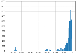
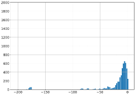
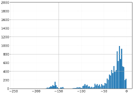
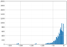
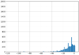
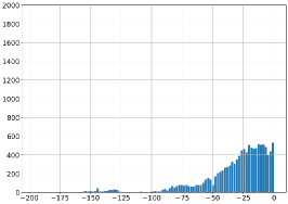
A.8.1 Curvature Distributions

Refer to caption
Refer to caption
Refer to caption
Refer to caption
Refer to caption
Refer to caption
Figure 3: AFRC distributions of edges in the Cora and Citeseer networks with no preprocessing (left), dropedge with $p=0.5$ (center), and AFR-3 using our heuristics (right).

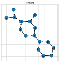
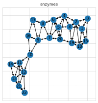
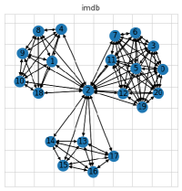
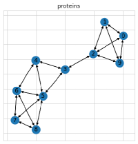
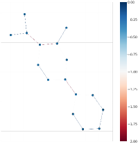
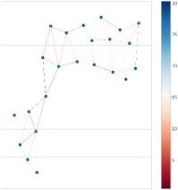
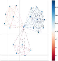
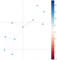
A.8.2 Example Graphs

Refer to caption
Refer to caption
Refer to caption
Refer to caption
Refer to caption
Refer to caption
Refer to caption
Refer to caption
Figure 4: Example networks from the mutag, enzymes, imdb, and proteins datasets, which we use for graph classification. The second row shows the same example networks with their edges colored according to their $\mathcal{AF}_{3}$ values.

A.9 Statistics for datasets

A.9.1 General statistics for node classification datasets

CORN. TEX. WISCON. CORA CITE. CHAM. COCO PAS.
# Graphs 1 1 1 1 1 1 123286 11355
#NODES 140 135 184 2485 2120 832 260-500 395-500
#EDGES 219 251 362 5069 3679 12355 1404-2924 2198-2890
# FEATURES 1703 1703 1703 1433 3703 2323 14* 14*
#CLASSES 5 5 5 7 6 5 81 21
DIRECTED TRUE TRUE TRUE FALSE FALSE TRUE FALSE FALSE
Table 24: Statistics of node classification datasets. *See Dwivedi et al. (2022) for details on LRGB datasets.

A.9.2 Curvature distributions for node classification datasets

$\mathcal{AF}_{3}$ $\mathcal{AF}_{4}$
DATASET MIN. MAX. MEAN STD MIN. MAX. MEAN STD CORR.
CORA -176 7 -15.039 31.102 -174 193 -6.534 30.826 0.876
CITESEER -108 10 -7.519 15.998 -100 429 4.769 29.392 0.156
TEXAS -106 3 -38.189 45.789 -103 97 -30.589 46.817 0.941
CORNELL -96 6 -32.371 41.795 -93 48 -27.614 43.432 0.941
WISCONSIN -127 4 -35.045 50.012 -122 62 -24.075 51.652 0.967
COCO $-8.1$ $3$ $-1.962$ $1.424$ $-1.7$ $26.6$ $7.853$ $2.674$ $0.407$
PASCAL $-8.1$ $2.9$ $-1.984$ $1.452$ $-1.3$ $24$ $7.759$ $2.502$ $0.419$
Table 25: Curvature statistics of node classification datasets.

A.9.3 General statistics for graph classification datasets

ENZYMES IMDB MUTAG PROTEINS PEPTIDES
#GRAPHS 600 1000 188 1113 15535
#NODES 2-126 12-136 10-28 4-620 8-444
#EDGES 2-298 52-2498 20-66 10-2098 10-928
AVG #NODES 32.63 19.77 17.93 39.06 150.94
AVG #EDGES 124.27 193.062 39.58 145.63 307.30
#CLASSES 6 2 2 2 10
DIRECTED FALSE FALSE FALSE FALSE FALSE
Table 26: Statistics of graph classification datasets.

A.9.4 Curvature distributions for graph classification datasets

$\mathcal{AF}_{3}$ $\mathcal{AF}_{4}$
DATASET MIN. MAX. MEAN STD MIN. MAX. MEAN STD CORR.
MUTAG -2.005 0.063 -0.881 0.773 -2.005 0.063 -0.881 0.773 1
ENZYMES -5.152 4.570 -0.273 2.230 -3.182 20.258 6.448 4.923 0.687
IMDB -4.239 4.546 0.257 2.069 -2.173 19.395 6.673 4.553 0.720
PROTEINS -4.777 8.039 2.917 3.562 66.097 191.539 120.982 25.424 0.661
PEPTIDES -1.999 0.994 -0.671 0.773 -.1996 0.995 -0.671 0.773 0.999
Table 27: Curvature statistics of graph classification datasets.

Datasets. For node classification, we conduct our experiments on the publicly available CORA, CITESEER Yang et al. (2016), TEXAS, CORNELL, WISCONSIN Pei et al. (2020) and CHAMELEON Rozemberczki et al. (2019) datasets. For graph classification, we use the ENZYMES, IMDB, MUTAG and PROTEINS datasets from the TUDataset collection Morris et al. (2020). As a long-range task, we consider the PEPTIDES-FUNC dataset from the LRGB collection Dwivedi et al. (2022).

A.10 Hardware specifications and libraries

All experiments in this paper were implemented in Python using PyTorch, Numpy PyTorch Geometric, and Python Optimal Transport. Figures in the main text were created using inkscape.

We conducted our experiments on a local server with the specifications laid out in the following table.

COMPONENTS SPECIFICATIONS
ARCHITECTURE X86_64
OS UBUNTU 20.04.5 LTS x86_64
CPU AMD EPYC 7742 64-CORE
GPU NVIDIA A100 TENSOR CORE
RAM 40GB
Table 28: