Kinematics-aware Trajectory Generation and Prediction with
Latent Stochastic Differential Modeling

Abstract

Trajectory generation and trajectory prediction are two critical tasks for autonomous vehicles, which generate various trajectories during development and predict the trajectories of surrounding vehicles during operation, respectively. However, despite significant advances in improving their performance, it remains a challenging problem to ensure that the generated/predicted trajectories are realistic, explainable, and physically feasible. Existing model-based methods provide explainable results, but are constrained by predefined model structures, limiting their capabilities to address complex scenarios. Conversely, existing deep learning-based methods have shown great promise in learning various traffic scenarios and improving overall performance, but they often act as opaque black boxes and lack explainability. In this work, we integrate kinematic knowledge with neural stochastic differential equations (SDE) and develop a variational autoencoder based on a novel latent kinematics-aware SDE (LK-SDE) to generate vehicle motions. Our approach combines the advantages of both model-based and deep learning-based techniques. Experimental results demonstrate that our method significantly outperforms baseline approaches in producing realistic, physically-feasible, and precisely-controllable vehicle trajectories, benefiting both generation and prediction tasks.

I Introduction

Trajectory prediction and generation are critical tasks for autonomous vehicles. First, as a key component in the autonomous driving pipeline, the trajectory prediction module predicts the future trajectories of surrounding vehicles based on their recent trajectory histories (as observed by the ego vehicle) and the map information. The prediction result provides a safe operation space for downstream behavioral-level decision-making and motion planning [1, 2, 3, 4, 5] and is critical for vehicle safety during operation. Furthermore, given the long-tailed nature of real traffic scenarios, it is important to conduct trajectory generation to augment trajectories collected in operation with additional synthetic but realistic trajectories, for testing and optimizing the planners [6, 7]. For instance, as shown in Fig. 1, we can convert a common and simple scenario to various challenging scenarios in the simulation by generating diverse trajectories and use them to test the reaction of the autonomous vehicle.

Most existing works focus on improving the average accuracy for trajectory prediction and enumerating various scenarios for trajectory generation. However, the predicted/generated trajectories may not be realistic or even physically feasible in real traffic scenarios, and lead to inferior training of the planning module and reduced capability to address safety-critical scenarios in practice. It is thus very important to ensure that the predicted/generated trajectories not only reflect the rich contextual factors, including other vehicles and HD maps, but also conform to traffic rules and fundamental laws of physics.

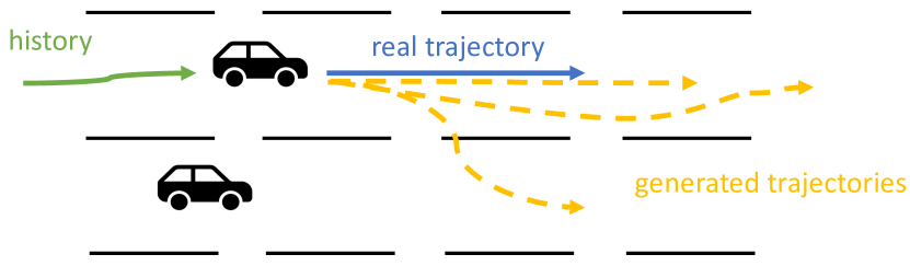
Figure 1: Generating diverse, physically-feasible, and explainable trajectories are important for critical scenario augmentation and vehicle motion prediction.

It is challenging for the trajectory predictor and generator to learn the representation of high-dimensional context while aligning with physical constraints. Traditional model-based techniques leverage simplified kinematic models, e.g., bicycle models, for trajectory generation. However, these methods provide a very rough estimation of vehicle’s real motion and oversimplify the environment model without considering the surroundings, leading to coarse-grained and maladaptive generated trajectories in complex traffic scenarios. On the other hand, learning-based generative models can well perceive the high-dimensional environment by learning from trajectory data and map context, as shown in recent advancements in trajectory prediction [8, 9, 10, 11] and generation [12, 13, 14, 15]. However, due to the lack of consideration of physical models, these generative techniques have little control over finer-grained vehicle-level kinematics and may produce unrealistic, physically-infeasible trajectories in real traffic scenarios.

In this paper, we aim to address the fundamental challenge in simultaneously considering the surrounding environment and vehicle physical model for trajectory generation and prediction. The major difficulty is from the conflict between high-dimensional environment (captured by deep learning) and low-dimensional physics. To address this, we utilize latent kinematics-aware neural stochastic differential equations (LK-SDE) to bridge the model-based kinematics and high-dimensional representations for road contexts in the latent space of a variational autoencoder (VAE). Specifically, we first extract the GCN representation from the HD maps and the environment, which convey the information of the environment contexts. Together with a physical model, the GCN representation is then used to train a neural SDE. Such kinematics-aware SDE is optimized and calculated in the latent space of the VAE, providing additional critical information for prediction and precise control for decoding the trajectory generation. It is worth noting that this architecture can be added to various scenario augmentation and trajectory prediction frameworks to enhance physical feasibility and explainability.

Our contributions are summarized as follows:

• We design a trajectory generator based on kinematics-guided SDE in the latent space, which effectively embeds physical constraints into deep learning models.

• For the trajectory generation task, compared with pure deep learning-based and model-based methods, our method can generate more realistic, explainable, and physically-feasible augmented trajectories by manipulating the kinematics-aware latent space.

• For the trajectory prediction task, our method can jointly predict physically-feasible trajectories and important kinematic states that are difficult to directly observe.

• Extensive experiments show that our method can outperform baseline methods in different metrics including smoothness, physical feasibility, and explainability. These improvements will benefit the augmentation of safety-critical scenarios and the prediction of future motions.

This paper is organized as follows. Section II introduces the background of trajectory generation and prediction and neural SDE. Section III presents the design of our LK-SDE based VAE for trajectory generation and prediction. Experiment results are shown in Section IV and Section V concludes the paper.

II Background

II-A Trajectory Generation and Prediction

Trajectory generation or augmentation plays an important role in evaluating and optimizing the decision-making module in autonomous driving. Many works use various deep learning methods to generate trajectories and scenarios. [13] proposes a VAE-conditioned method to bridge safe and collision-driving data to generate the whole risky scenario, but it cannot control agent-level trajectories. [12] designs a GAN-based method - RouteGAN to generate diverse trajectories for every single agent and the trajectory is controlled by a style variable. Recent works [14, 15, 16] further utilize domain knowledge such as causal relation and traffic prior to generating useful traffic scenarios. However, these methods mainly focus on scenario-level generation. For trajectory generation of a single vehicle, these works still rely on pure deep learning methods or model-based methods. The latent spaces of these generative methods are not well modeled or explained for a single vehicle, especially at the kinematics or dynamics level. The models only have coarse and limited control over the generated trajectories, which may lead to physically-infeasible and uncontrollable trajectories.

Recent works applied advanced deep learning techniques to learn the representations of agents’ trajectories and road contexts. Graph neural networks [9, 17] and transformer [8, 11] are used to extract context features. [18] adds a bicycle model after the neural feature extractor to decode the trajectories but their pure model-based decoder still suffers from the oversimplification of the vehicle motion. In our work, we aim to combine the powerful representations from deep learning models with kinematics knowledge in the latent space.

II-B Neural Stochastic Differential Equation

The physical dynamics of many real-world systems can be modeled as a discrete-time SDE [19]. An SDE is a differential equation that contains stochastic processes, which can be expressed as

$$\mathbf{s}_{t+1}=f(\mathbf{s}_{t})+g(\mathbf{s}_{t})W(t)$$

where $\mathbf{s}_{t}\in\mathbb{R}^{n}$ is the system state, $f:\mathbb{R}^{n}\rightarrow\mathbb{R}^{n}$ denotes a drift function and $g:\mathbb{R}^{n}\rightarrow\mathbb{R}^{n\times d}$ represents a diffusion function, $W(t)\in\mathbb{R}^{d}$ is the Brownian Motion (also known as Wiener Process), for encoding the stochasticity in the systems. A neural SDE is an SDE with its drift function and diffusion function as neural networks, e.g., $f_{\theta},g_{\theta}$ [20].

To learn such neural network representations, a typical way is to sample the environment and neural SDE to generate the trajectory data $\tau=\{\mathbf{s}_{0},\mathbf{s}_{1},\cdots,\mathbf{s}_{T}\}$, and $\hat{\tau}_{\theta}=\{\hat{\mathbf{s}}_{0},\hat{\mathbf{s}}_{1},\cdots,\hat{\mathbf{s}}_{T}\}$ respectively. Then fit the real-world trajectory $\tau$ to the neural networks by reducing the following loss function:

$$\min_{\theta}\mathcal{L}(\tau,\hat{\tau}_{\theta})=\min_{\theta}-\sum_{t=0}^{T}\log\left(P\left(\mathbf{s}_{t}~{}|~{}\mathcal{N}(\hat{\mathbf{s}}_{t},g_{\theta}(\hat{\mathbf{s}}_{t})\right)\right)$$

where $\mathcal{L}$ is the maximum likelihood loss, $T$ is the time length of prediction and generation, $P\left(\mathbf{s}_{t}~{}|~{}\mathcal{N}(\hat{\mathbf{s}}_{t},g_{\theta}(\hat{\mathbf{s}}_{t})\right)$ is the likelihood probability of the observed $\mathbf{s}_{t}$ under the normal distribution of the neural SDE $\mathcal{N}(\hat{\mathbf{s}}_{t},g_{\theta}(\hat{\mathbf{s}}_{t}))$.

III Our LK-SDE Methods

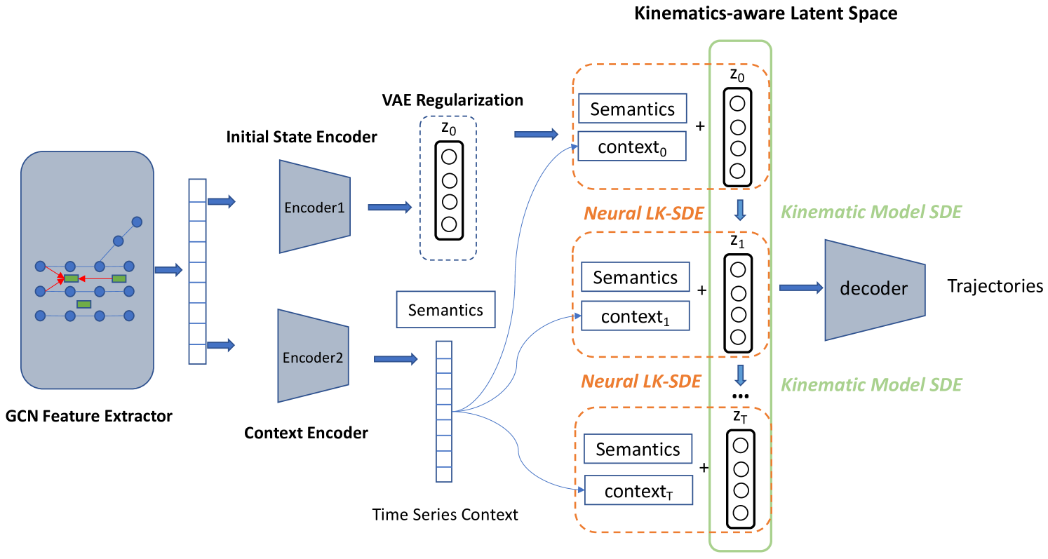
Figure 2: The overall design of our kinematics-aware trajectory generator. The orange boxes with dashed lines represent the inputs for our neural latent kinematics-aware SDE (LK-SDE), and the green box represents the transition process of the bicycle model. Our neural LK-SDE is guided by the kinematic bicycle model during training to learn physical knowledge for trajectory generation and prediction.

III-A Overall Design

Overview: Our method combines the deep learning-based feature extractors with kinematics-aware latent space by a physics-guided SDE solver. The overall architecture of the proposed method is shown in Fig. 2. We first feed the trajectories of vehicles and map contexts into a GCN-based feature extractor to learn representations of HD maps and interactions between vehicles. The extracted features are further processed by two encoders - one encoder converts the representations to a four-dimensional latent initial state; the other encoder will generate a global semantic vector and finer-grained time-series contexts for future steps in the latent space. Our LK-SDE will take the semantic vector, corresponding context, and the initial state as inputs and roll out latent states step by step. With the same initial latent state, a bicycle-model SDE also rolls out latent states. The LK-SDE states are guided to be close to the bicycle-model states and thus we embed the kinematics knowledge into the latent space, but the neural LK-SDE utilizes rich contexts and has more precise latent states. Finally, a simple fully connected neural network will decode the latent vectors into trajectory space.

Input & Output: The input for the entire model is the two-dimensional history trajectories of vehicles (including both target and surrounding vehicles) and the graph of HD maps. The output of the model is the generated or predicted future trajectories.

III-B Context Extraction and Embedding

Similar to [9], we use a one-dimensional convolutional network to model history trajectories for its effectiveness in extracting multi-scale features and efficiency in parallel computing. Multiple graph neural networks are utilized to learn the interactions among agents and lane nodes. After fusing the features of graphs and agents, we have two encoders to generate contexts and initial states for our LK-SDE, as is shown in Fig. 2. A ResNet[21] is applied in the context encoder to further generate global semantics and time-series local contexts for future time steps. Therefore, for each time step in the prediction horizon, we will have eight-dimensional local contexts $\mathbf{ctx}_{t}$ and four-dimensional global semantics $\mathbf{sem}$. In addition, parallel with the context encoder, we use a fully connected neural network (Initial state encoder in Fig. 2) to estimate the latent initial state for our LK-SDE and physical model. The latent initial state $\mathbf{z}_{0}$ is regularized to follow Gaussian distribution by minimizing the Kullback–Leibler divergence as shown in  1.

$$Loss_{reg}=KL(q(\mathbf{z}_{0}|x)||p(\mathbf{z}_{0})),$$ (1)

where $x$ is the input features, $p(\mathbf{z}_{0})$ represents the targeted distribution of the latent initial state (i.e. Gaussian distribution), and $q$ represents the posterior distribution from the initial state encoder. The initial latent states $\mathbf{z}_{0}$ will be the input for the following LK-SDE, and the global semantics $\mathbf{sem}$ as well as local contexts $\mathbf{ctx}$ will be the condition.

III-C Latent Kinematics Modeling

The generation and prediction of vehicle trajectories rely on understanding the inherent dynamics and physical laws governing these trajectories. Consequently, this compels us to focus on acquiring a latent space that is attuned to the kinematics. More specifically, within the scope of this work, our objective is to acquire a LK-SDE for the purposes of motion prediction and generation. This involves not only optimizing the loss function based on the ground truth label but also incorporating supervision from an explicit bicycle model [22], to serve as a constraint for the drift function within LK-SDE. Specifically, the kinematics-aware latent space modeling involves two SDEs during training - one is the bicycle-model-based SDE to generate the kinematics based on the most recent states; the other is the neural LK-SDE that we optimized to learn the kinematics from the bicycle model SDE and finally generate vehicle motion. The detailed kinematics-guided dual SDE learning process is illustrated in Fig. 3.

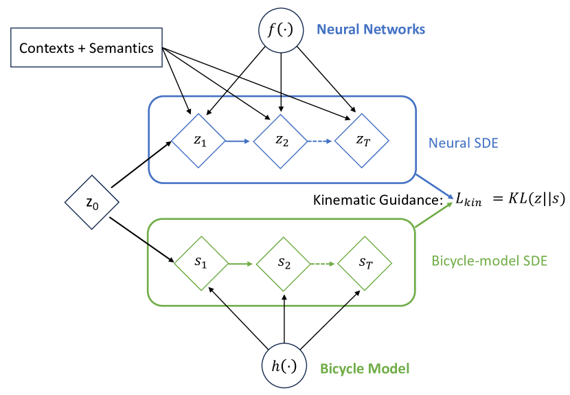
Figure 3: During the training, the bicycle model SDE guides our neural LK-SDE to follow the kinematics by minimizing the KL divergence between the solutions of two SDEs. The kinematic loss function $L_{kin}$ is explained in Eq. (4).

The bicycle-model-based SDE is designed with the intention of infusing a comprehensive understanding of physics into our neural LK-SDE. Over time, the latent state evolves according to this SDE, enabling us to capture a series of kinematics in the latent space of the VAE. This latent trajectory is subsequently decoded to produce the final task output, thereby increasing the likelihood of adhering to the specified physical constraints.

We assume the bicycle model SDE has $h(\mathbf{s}_{t},\pi)$ as its drift function, $g(\mathbf{s}_{t})$ as the diffusion coefficient matrix which is diagonal and shared by our LK-SDE. Therefore the bicycle model could be expressed as $\mathbf{s}_{t+1}=h(\mathbf{s}_{t},\pi)+g(\mathbf{s}_{t})W(t)$, where the drift function $h(\mathbf{s}_{t},\pi)$ is shown in the following equations (2).

$$x_{t+1} =x_{t}+\delta\cdot v_{t}\cos(\psi_{t}+\beta(u_{2})),$$ (2)

$$y_{t+1} =y_{t}+\delta\cdot v_{t}\sin(\psi_{t}+\beta(u_{2})),$$

$$v_{t+1} =v_{t}+\delta\cdot u_{1}$$

$$\psi_{t+1} =\psi_{t}+\delta\cdot\frac{v_{t}}{l_{r}}\sin(\beta(u_{2})),$$

$$\beta(u_{2}) =\arctan\left(\tan(u_{2})\frac{l_{r}}{l_{f}+l_{r}}\right),$$

$$(u_{1},u_{2}) =\pi(\mathbf{s}_{t})$$

where the state vector $\mathbf{s}_{t}=(x_{t},y_{t},v_{t},\psi_{t})$ represents the lateral position, longitudinal position, velocity, and yaw angle, respectively. $\beta$ is the slip angle, and $l_{f},l_{r}$ are the distances between the car center and the front, and rear axle, respectively. $\delta>0$ is a small sampling period. The control inputs correspond to the acceleration $u_{1}$ and front wheel steering angle $u_{2}$. We implement a learnable feedback neural controller $\pi$ to generate the control inputs as $u_{1},u_{2}=\pi(\mathbf{s}_{t})$, and therefore the bicycle model SDE is an autonomous system evolving with the dynamics $h(\cdot,\pi),g(\cdot)$. A detailed illustration of the model is shown in Fig. 4.

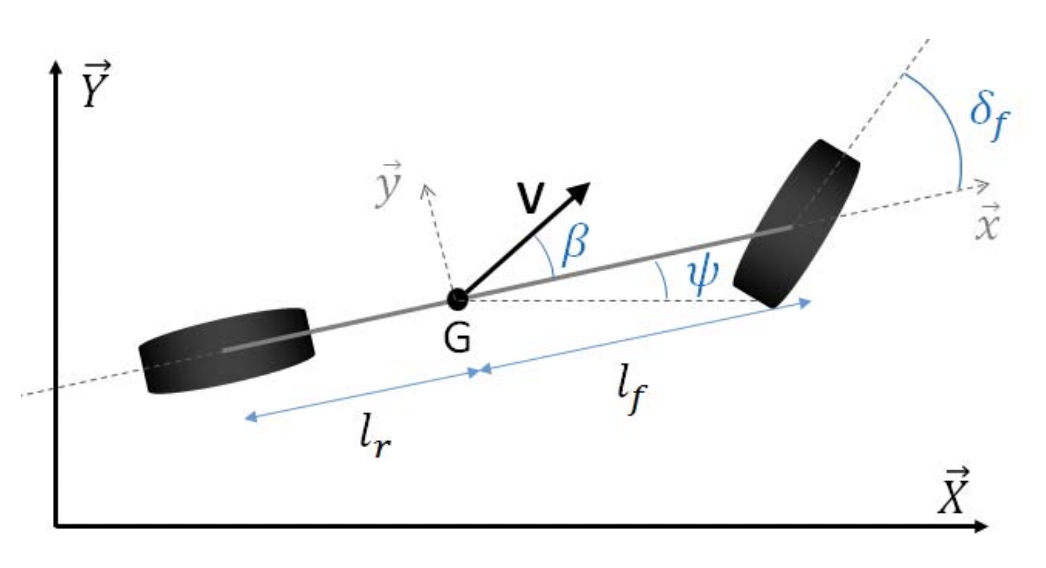
Figure 4: Illustration of the bicycle model[22].

For our LK-SDE, the inputs for the neural network drift function $f$ are the latent states from the last time step, the global semantics, and local contexts. Following the transition function as shown in Eq. (3), our LK-SDE will generate the kinematics-aware vectors $\mathbf{z}$ for every time step in the latent space of the VAE.

$$\mathbf{z}_{t+1}=f(\mathbf{z}_{t},\mathbf{sem},\mathbf{ctx}_{t})+g(\mathbf{z}_{t})W(t)$$ (3)

To embed the kinematic knowledge from the bicycle model SDE to LK-SDE, we minimize the KL divergence between the solutions $\mathbf{z},\mathbf{s}$ to two SDEs, similar to Equation 10 in torchsde [20] and Appendix B in [23].

$$L_{kin}=KL(\mathbf{z}||\mathbf{s})=$$ (4)

$$\sum_{t=0}^{T}\mathbb{E}_{W(t)}\left[\frac{1}{2}\norm{\biggl{(}g^{-1}\left(f(\mathbf{z}_{t},\mathbf{sem},\mathbf{ctx}_{t})-h(\mathbf{s_{t}},\pi)\right)\biggr{)}}^{2}_{2}\right]$$

where $T$ is the time length of the training trajectory segment. Same with the previous definition, $g(\mathbf{s}_{t})$ is the diagonal and shared diffusion coefficient matrix in our LK-SDE and bicycle model SDE. Basically, we enforce the neural drift function $f(\mathbf{z}_{t},\mathbf{sem},\mathbf{ctx}_{t})$ to get close to the bicycle model $h(\mathbf{z}_{t},\pi)$, as shown in Fig 3. In the training, we leverage batch size to compute and reduce the sample mean for this loss function.

III-D Optimization Pipeline

To regularize the latent space and generate the final trajectories, we need to optimize and balance several loss functions. We update the feature extractor and initial state encoder by the VAE regularization loss as shown in Eq. (1), in order to make the latent space follow Gaussian distribution. The two SDEs, feature extractor and encoders are optimized to embed the kinematic knowledge into latent vectors by $L_{kin}$ in Eq. (4). After the latent space modeling, a neural network decoder $D$ projects the latent vectors back into the observation space. Finally, the whole pipeline is optimized by a smooth L1 loss as shown in Eq. (5) to minimize the distance between output trajectories $\hat{o}$ and the ground truth $o$ we collected in the real world.

$$Loss_{pred}\left(o_{i},\hat{o_{i}}\right)=\begin{cases}0.5(o_{i}-\hat{o_{i}})^{2}&\text{ if }\left\|o_{i}-\hat{o_{i}}\right\|<1\\ \left\|o_{i}-\hat{o_{i}}\right\|-0.5&\text{ otherwise }\end{cases}$$ (5)

The detailed optimization process during training is demonstrated in Alg. 1.

Algorithm 1 Optimization Pipelines

1:  Initialize: feature extractor $G$, initial state encoder $E_{s}$, context encoder $E_{c}$, decoder $D$, LK-SDE($f$,$g$), and bicycle-model SDE($h$,$g$)

2:  Input: past trajectories $t$ and map graph $m$.

3:  for each batch do

4:     Let features $x$ = $G(t,m)$.

5:     Let initial kinematic vectors $\mathbf{z}_{0}$ = $\mathbf{s}_{0}$ = $E_{s}(x)$.

6:     Let global semantics and time series contexts$\mathbf{sem}$ , $\mathbf{ctx}_{1,2,...,T}$ = $E_{c}(x)$

7:     Update the $G$ and $E_{s}$ by the regularization loss $L_{reg}$ (1).

8:     for each time step do

9:        LK-SDE computes $\mathbf{z}_{t+1}=f(\mathbf{z}_{t},\mathbf{ctx}_{t},\mathbf{sem})+g(\mathbf{z}_{t})W(t)$

10:        Bicycle model SDE computes $\mathbf{s}_{t+1}=h(\mathbf{s}_{t},\pi)+g(\mathbf{s}_{t})W(t)$.

11:     end for

12:     Update the LK-SDE ($f$,$g$) and $\pi$ by the kinematic loss $L_{kin}$ (4).

13:     The decoder projects latent vectors into trajectory space $\hat{o}=D(\mathbf{z}_{0},\mathbf{z}_{1},\cdots,\mathbf{z}_{T})$

14:     Update the $G$, $E_{s}$, $E_{c}$, LK-SDE ($f$,$g$) by the prediction loss $L_{pred}$ (5).

15:  end for

IV Experiments

In this section, we conduct extensive experiments to evaluate the proposed methods. The data and training settings are introduced in Sec. IV-A. We demonstrate our methods can generate smoother and more controllable augmented trajectories than baselines via visualized and statistical comparison in Sec. IV-B. Furthermore, in Sec. IV-C, we compare our approach with model-based methods and state-of-the-art pure deep learning methods on prediction accuracy which is an important metric for representation learning.

IV-A Experiment Settings

We train our model on the Argoverse motion forecasting dataset [24] and evaluate the generation and prediction performance on its validation set. The benchmark has more than 30K scenarios collected in Pittsburgh and Miami. Each scenario has a graph of the road map and trajectories of agents sampled at 10 Hz. In the motion generation and prediction tasks, we use the first 2 seconds of trajectories as input and generate the subsequent 3-second trajectories.

IV-B Controllable and Realistic Trajectory Generation

Generative models are commonly used to augment or generate more realistic and safety-critical trajectories for simulation and evaluation. We can generate trajectories by tuning the latent space of the generative model such as VAE, GAN, and our LK-SDE. We compare our methods with the learning-based generative model - TAE [16] and the bicycle-model-based DKM [18]. To measure the smoothness of the generative trajectories, we applied the metrics of turning rate and jerk. The jerk is the rate of change of an object’s acceleration over time (the definition is Eq. (6)) and the magnitude of jerk is commonly used to represent the smoothness of trajectories [25, 26]. According to [25], the jerk threshold for discomfort presents about $0.3~{}m/s^{3}$, ranging up to $0.9~{}m/s^{3}$. In our work, we consider trajectories with jerks exceeding $0.9~{}m/s^{3}$ as violations.

$$\mathbf{j}(t)=\frac{\mathrm{d}\mathbf{a}(t)}{\mathrm{d}t}=\frac{\mathrm{d}^{2}\mathbf{v}(t)}{\mathrm{d}t^{2}}=\frac{\mathrm{d}^{3}\mathbf{x}(t)}{\mathrm{d}t^{3}}$$ (6)

As shown in Table I, our LK-SDE based model has the lowest average jerk value and average absolute turning rate[18], indicating our methods can generate smoother and more realistic trajectories than DKM and TAE. Specifically, in Fig. 5, TAE generates trajectories with sparse and unstable jerks - about 26% trajectories are with jerk magnitude above the discomfort threshold ($0.9~{}m/s^{3}$), showing the difficulty of smooth trajectory generation by DL methods. For DKM, there are 8.7% of generated trajectories have higher jerk values than the threshold. Our LK-SDE based model generates the smoothest and most stable vehicle motions with only a 5.0% violation rate.

TABLE I: Smoothness comparison between our LK-SDE based model and baselines including TAE and DKM.

	Jerk($m/s^{3}$)	Violation Rate	Turning Rate($rad/s$)
TAE (DL-based) [16]	$0.64$	$26\%$	$0.025$
DKM (Model-based) [18]	$0.43$	$8.7\%$	$0.022$
LK-SDE (Ours)	0.40	5.0%	0.009

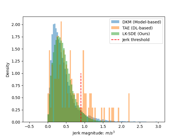
Figure 5: The distribution of the jerk magnitude of different generative methods. The red dashed line represents the discomfort threshold for jerk value. We notice that our proposed LK-SDE can augment the smoothest and most stable trajectories.

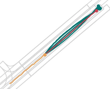
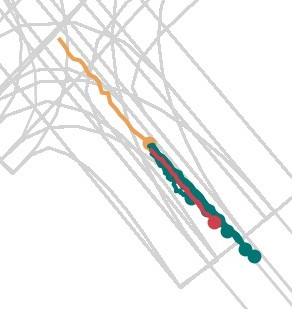
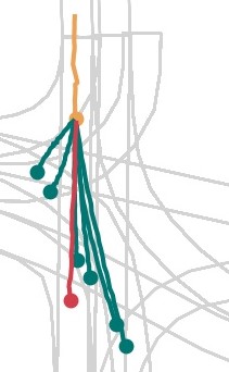
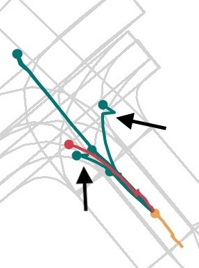
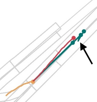
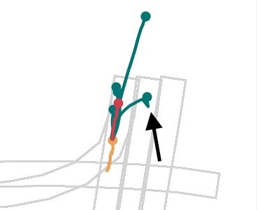
Figure 6: Visualization of the augmented trajectories. The top row shows the trajectories generated by our LK-SDE model. We manually tune the initial values in the latent space (lateral for (a), longitudinal for (b), and yaw angle for (c)). The bottom row shows trajectories generated by the pure deep learning method - TAE by tuning its behavior latent space (lateral for (d), longitudinal for (e), random for (f)). In all the subplots, the orange lines are history trajectories, the red lines are ground truth for future motion, green lines are augmented trajectories. The black arrows point to the parts of trajectories that are obviously physically infeasible or unrealistic by TAE. The generated trajectories in (a)(b)(c) visually align with the physical knowledge from the bicycle model, showing the effectiveness of our LK-SDE design.

The top row in Fig. 6 illustrates that our LK-SDE model can accurately augment smooth and realistic vehicle motions in an explainable and controllable manner. We tune the initial states for lateral direction, longitudinal direction, and yaw angle, respectively. We find that many trajectories generated by TAE (bottom row in Fig. 6) have unrealistic and physically-infeasible motions such as sharp turns and sudden offsets.

IV-C Accurate and Explainable Trajectory Representation and Prediction

In addition to the ability of trajectory augmentation, motion prediction is also an important task for environmental understanding and decision-making. The accuracy of trajectory prediction is a suitable metric to measure the ability to learn the representation of the environment and generate realistic trajectories. Generally, the average performance of trajectory prediction or regression is measured by average displacement error (ADE, defined as the average of the root mean squared error between the predicted waypoints and the ground-truth trajectory waypoints) and the final displacement error (FDE, defined as the root mean squared error between the last predicted waypoint and the last ground-truth trajectory waypoint). We compare our methods with the DL-based GRIP++ [27], LaneGCN [9], and TPCN [10], domain knowledge aware generative methods TAE[16], and bicycle-model-based DKM[18]. The results in Tab. II show that our LK-SDE model outperforms GRIP++, DKM, TAE, and achieves similar performance to the state-of-the-art LaneGCN and TPCN. Combining the results from trajectory generation and augmentation, we can conclude that our latent kinematics-aware SDE can learn the representation of trajectories and environments more effectively than the model-based methods and generate smoother and more controllable motions than the DL-based generative models. In addition to the average accuracy, our methods can also give detailed and accurate kinematics prediction (e.g. steering angle) along with the waypoints, which provide more explainable information for safety-critical decision-making.

TABLE II: Trajectory prediction comparison between our LK-SDE model and baselines.

	ADE$\downarrow$	FDE$\downarrow$
GRIP++[27]	$1.77$	$3.91$
LaneGCN[9]	$1.35$	$2.96$
TPCN[10]	$1.34$	$2.95$
TAE [16]	$1.42$	$3.08$
DKM [18]	$1.46$	$3.14$
LK-SDE (Ours)	$1.39$	$2.98$

V Conclusion

In this work, we propose trajectory generation and prediction based on the latent kinematics-aware stochastic differential equation (LK-SDE). We embed the physics knowledge into the latent space of a VAE by the dual SDE design. The method can bridge the high-dimensional features from the environment and the low-dimensional kinematics to make generated trajectories fine-grained, physically feasible, and precisely explainable.

References

- [1] X. Liu, R. Jiao, Y. Wang, Y. Han, B. Zheng, and Q. Zhu, “Safety-assured speculative planning with adaptive prediction,” arXiv preprint arXiv:2307.11876, 2023.
- [2] Y. Hu, J. Yang, L. Chen, K. Li, C. Sima, X. Zhu, S. Chai, S. Du, T. Lin, W. Wang, et al., “Planning-oriented autonomous driving,” in Proceedings of the IEEE/CVF Conference on Computer Vision and Pattern Recognition, 2023, pp. 17 853–17 862.
- [3] R. Jiao, H. Liang, T. Sato, J. Shen, Q. A. Chen, and Q. Zhu, “End-to-end uncertainty-based mitigation of adversarial attacks to automated lane centering,” in 2021 IEEE Intelligent Vehicles Symposium (IV). IEEE, 2021, pp. 266–273.
- [4] R. Jiao, X. Liu, T. Sato, Q. A. Chen, and Q. Zhu, “Semi-supervised semantics-guided adversarial training for trajectory prediction,” arXiv preprint arXiv:2205.14230, 2022.
- [5] X. Liu, C. Huang, Y. Wang, B. Zheng, and Q. Zhu, “Physics-aware safety-assured design of hierarchical neural network based planner,” in 2022 ACM/IEEE 13th International Conference on Cyber-Physical Systems (ICCPS). IEEE, 2022, pp. 137–146.
- [6] W. Ding, C. Xu, M. Arief, H. Lin, B. Li, and D. Zhao, “A survey on safety-critical driving scenario generation—a methodological perspective,” IEEE Transactions on Intelligent Transportation Systems, 2023.
- [7] J. Cai, W. Deng, H. Guang, Y. Wang, J. Li, and J. Ding, “A survey on data-driven scenario generation for automated vehicle testing,” Machines, vol. 10, no. 11, p. 1101, 2022.
- [8] Y. Liu, J. Zhang, L. Fang, Q. Jiang, and B. Zhou, “Multimodal motion prediction with stacked transformers,” in Proceedings of the IEEE/CVF Conference on Computer Vision and Pattern Recognition, 2021, pp. 7577–7586.
- [9] M. Liang, B. Yang, R. Hu, Y. Chen, R. Liao, S. Feng, and R. Urtasun, “Learning lane graph representations for motion forecasting,” in European Conference on Computer Vision. Springer, 2020, pp. 541–556.
- [10] M. Ye, T. Cao, and Q. Chen, “Tpcn: Temporal point cloud networks for motion forecasting,” in Proceedings of the IEEE/CVF Conference on Computer Vision and Pattern Recognition, 2021, pp. 11 318–11 327.
- [11] Y. Yuan, X. Weng, Y. Ou, and K. M. Kitani, “Agentformer: Agent-aware transformers for socio-temporal multi-agent forecasting,” in Proceedings of the IEEE/CVF International Conference on Computer Vision, 2021, pp. 9813–9823.
- [12] Z.-H. Yin, L. Sun, L. Sun, M. Tomizuka, and W. Zhan, “Diverse critical interaction generation for planning and planner evaluation,” in 2021 IEEE/RSJ International Conference on Intelligent Robots and Systems (IROS). IEEE, 2021, pp. 7036–7043.
- [13] W. Ding, M. Xu, and D. Zhao, “Cmts: A conditional multiple trajectory synthesizer for generating safety-critical driving scenarios,” in 2020 IEEE International Conference on Robotics and Automation (ICRA). IEEE, 2020, pp. 4314–4321.
- [14] W. Ding, H. Lin, B. Li, and D. Zhao, “Causalaf: causal autoregressive flow for safety-critical driving scenario generation,” in Conference on Robot Learning. PMLR, 2023, pp. 812–823.
- [15] D. Rempe, J. Philion, L. J. Guibas, S. Fidler, and O. Litany, “Generating useful accident-prone driving scenarios via a learned traffic prior,” in Proceedings of the IEEE/CVF Conference on Computer Vision and Pattern Recognition, 2022, pp. 17 305–17 315.
- [16] R. Jiao, X. Liu, B. Zheng, D. Liang, and Q. Zhu, “Tae: A semi-supervised controllable behavior-aware trajectory generator and predictor,” arXiv preprint arXiv:2203.01261, 2022.
- [17] H. Zhao, J. Gao, T. Lan, C. Sun, B. Sapp, B. Varadarajan, Y. Shen, Y. Shen, Y. Chai, C. Schmid, et al., “Tnt: Target-driven trajectory prediction,” arXiv preprint arXiv:2008.08294, 2020.
- [18] H. Cui, T. Nguyen, F.-C. Chou, T.-H. Lin, J. Schneider, D. Bradley, and N. Djuric, “Deep kinematic models for kinematically feasible vehicle trajectory predictions,” in 2020 IEEE International Conference on Robotics and Automation (ICRA). IEEE, 2020, pp. 10 563–10 569.
- [19] P. E. Kloeden, E. Platen, P. E. Kloeden, and E. Platen, Stochastic differential equations. Springer, 1992.
- [20] X. Li, T.-K. L. Wong, R. T. Chen, and D. Duvenaud, “Scalable gradients for stochastic differential equations,” in International Conference on Artificial Intelligence and Statistics. PMLR, 2020, pp. 3870–3882.
- [21] K. He, X. Zhang, S. Ren, and J. Sun, “Deep residual learning for image recognition,” in Proceedings of the IEEE conference on computer vision and pattern recognition, 2016, pp. 770–778.
- [22] P. Polack, F. Altché, B. d’Andréa Novel, and A. de La Fortelle, “The kinematic bicycle model: A consistent model for planning feasible trajectories for autonomous vehicles?” in 2017 IEEE intelligent vehicles symposium (IV). IEEE, 2017, pp. 812–818.
- [23] P. Kidger, J. Foster, X. C. Li, and T. Lyons, “Efficient and accurate gradients for neural sdes,” Advances in Neural Information Processing Systems, vol. 34, pp. 18 747–18 761, 2021.
- [24] M.-F. Chang, J. Lambert, P. Sangkloy, J. Singh, S. Bak, A. Hartnett, D. Wang, P. Carr, S. Lucey, D. Ramanan, et al., “Argoverse: 3d tracking and forecasting with rich maps,” in Proceedings of the IEEE/CVF Conference on Computer Vision and Pattern Recognition, 2019, pp. 8748–8757.
- [25] I. Bae, J. Moon, J. Jhung, H. Suk, T. Kim, H. Park, J. Cha, J. Kim, D. Kim, and S. Kim, “Self-driving like a human driver instead of a robocar: Personalized comfortable driving experience for autonomous vehicles,” arXiv preprint arXiv:2001.03908, 2020.
- [26] A. Scamarcio, P. Gruber, S. De Pinto, and A. Sorniotti, “Anti-jerk controllers for automotive applications: A review,” Annual Reviews in Control, vol. 50, pp. 174–189, 2020.
- [27] X. Li, X. Ying, and M. C. Chuah, “Grip++: Enhanced graph-based interaction-aware trajectory prediction for autonomous driving,” arXiv preprint arXiv:1907.07792, 2019.