Connectivity of Random Geometric Hypergraphs

Abstract

We consider a random geometric hypergraph model based on an underlying bipartite graph. Nodes and hyperedges are sampled uniformly in a domain, and a node is assigned to those hyperedges that lie with a certain radius. From a modelling perspective, we explain how the model captures higher order connections that arise in real data sets. Our main contribution is to study the connectivity properties of the model. In an asymptotic limit where the number of nodes and hyperedges grow in tandem we give a condition on the radius that guarantees connectivity.

1 Motivation

There is growing interest in the development of models and algorithms that capture group-level interactions [5, 6, 28]. For example, multiple co-authors may be involved in a collaboration, multiple workers may share an office space, and multiple proteins may contribute in a cellular process. In such cases representing the connectivity via a network of pairwise interactions is an obvious, and often avoidable, simplification. Hypergraphs, where any number of nodes may be grouped together to form a hyperedge, form a natural generalization. Hypergraph-based techniques have been developed for

• studying the propagation of disease or information [1, 4, 7, 18, 19, 20],

• investigating the importance or structural roles of individual components [12, 30, 29],

• discovering and quantifying clusters [8, 27, 13],

• predicting future connections [33, 32],

• inferring connectivity structure from time series data [21].

Just as in the pairwise setting, it is also of interest to consider processes that create hypergraphs [3, 15]. Comparing generative hypergraph models against real data sets may help us to understand the mechanisms through which interactions arise. Furthermore, realistic models can be used to produce synthetic data sets on which to base simulations, and also to form null models for studying features of interest.

Models that use a geometric construction, with connectivity between elements determined by distance, have proved useful in many settings. Random geometric graphs were first introduced in [14] to model communication between radio stations, although the author also mentioned their relevance to the spread of disease. These models have subsequently proved useful in many application areas, ranging from studies of the proteome [16, 26, 17] to academic citations [31]. In many settings, the notion of distance may relate to an embedding of nodes into a latent space that captures key features. Here, similarity is interpreted in an indirect or abstract sense. Random geometric graphs have also been studied theoretically, with many interesting results arising from the perspectives of analysis, probability and statistical physics [22, 24, 10, 2, 25, 9]

Our aim in this work is motivate and analyse a random geometric hypergraph model. In a similar manner to [3], we make use of the connection between hypergraphs and bipartite graphs. The model is introduced and motivated in section 2, where we also show the results of illustrative computational experiments concerning connectivity. Our main contribution is to derive a condition on the thresholding radius that asymptotically guarantees connectivity of the hypergraph. The result is stated and proved in section 3. Directions for future work are described in section 4.

2 The Random Geometric Model and Its Connectivity

In this section we motivate and informally describe a geometric random hypergraph model, and computationally investigate its connectivity. We make use of a well known equivalence between hypergraphs and bipartite graphs [3, 11]. Suppose we are given an undirected bipartite graph, where nodes have been separated into two groups, A and B. By construction any edge must join one node in group A with one node in group B. We may form a hypergraph on the nodes in group A with the following rule:

• nodes in group A appear in the same hyperedge if and only if, in the underlying bipartite graph, they both have an edge to the same node in group B.

In this way the nodes in set B may be viewed as hyperedge “centres.” Two nodes from group A that are attracted to the same centre are allocated to the same hyperedge. In many graph settings there is a natural concept of distance between nodes. For example, in social networks, geographical distance between places of work or residence may play a strong role in determining connectivity. More generally, there may be a more nuanced set of features (hobbies, tastes in music, pet ownership, …) that help to explain whether pairwise relationships arise. This argument extends readily to the bipartite/hypergraph scenario. Hyperedge centres may correspond, for example, to shops, office buildings, gyms, train stations, restaurants, concert venues, churches,…, with an individual joining a hyperedge if they are sufficiently close to that centre; for example, exercising at a local gym. In the absence of specific information, it is natural to assume that the features possessed by a node arise at random, so that a node is randomly embedded in $\mathbb{R}^{d}$ for some dimension $d$. In a similar way, we may simultaneously embed our hyperedge centres in $\mathbb{R}^{d}$, and assign a node to a hyperedge if and only if it is within some threshold distance of the centre.

Figure 1 illustrates the idea in the two dimensional case. We have a bipartite graph with two types of nodes. Groups A and B are represented by circles and stars, respectively. We form a hypergraph by placing a circle node in a hyperedge if and only if it is within a certain distance of the corresponding star. Colours in the figure distinguish between the different hyperedges. We emphasize that mathematically the resulting hypergraph consists only of the list of hypergraph nodes and hyperedges. Information about the existence/number of hyperedge centres and the locations of all nodes in $\mathbb{R}^{2}$ is lost.

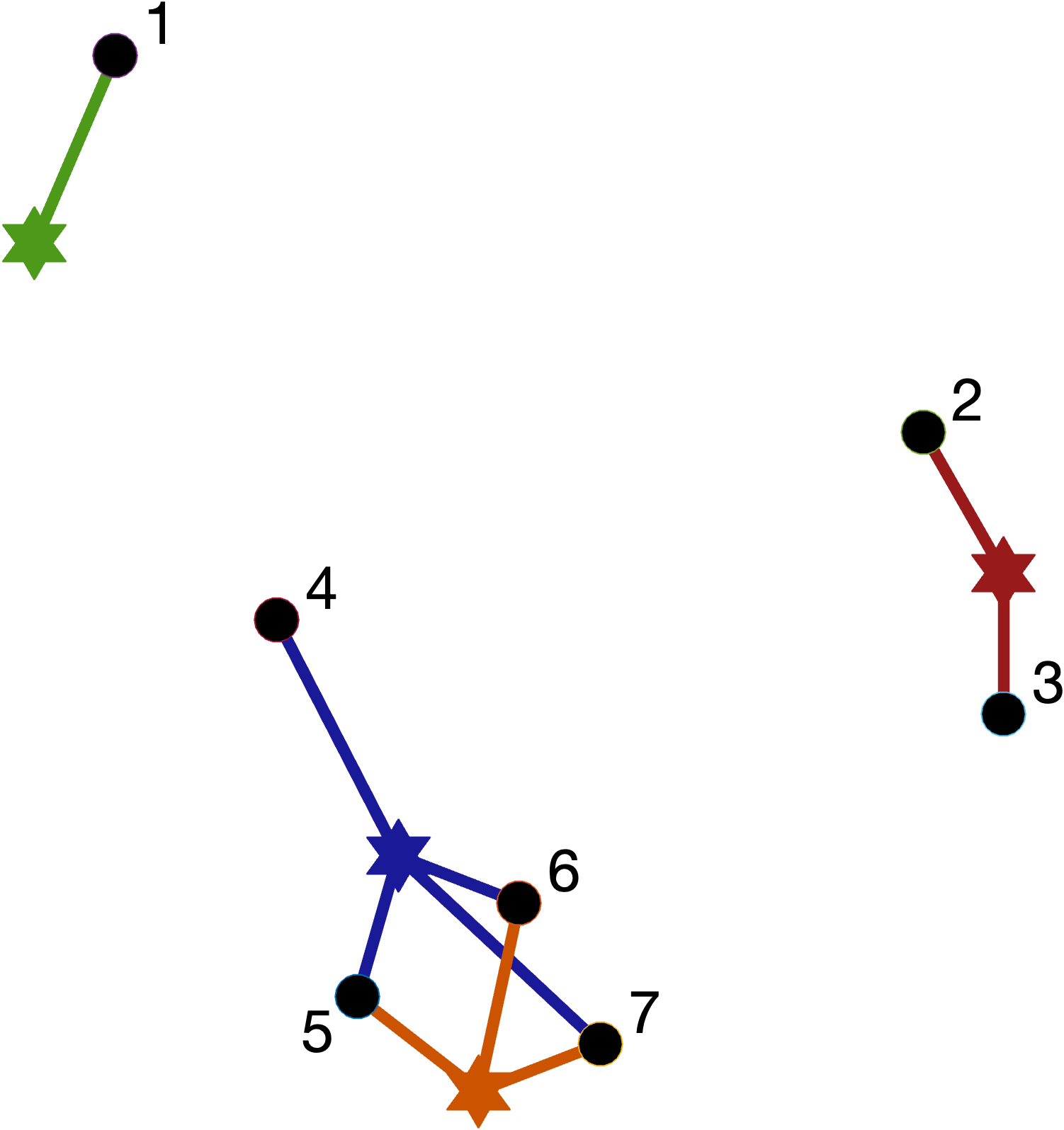
Figure 1: When this construction is regarded as a bipartite graph, the solid circles and solid stars represent two types of node. Edges are created only between nodes of a different type; this happens if any only if they are close enough in Euclidean distance. When regarded as a hypergraph, the solid circles represent nodes and the solid stars represent “centres” of hyperedges. A node is a member of a hyperedge if and only if it is sufficiently close to the corresponding centre. Mathematically, the resulting hypergraph may defined by labelling the nodes $\{1,2,3,4,5,6,7\}$ and listing the hyperedges as $\{1\}$, $\{2,3\}$, $\{4,5,6,7\}$ and $\{5,6,7\}$.

Our aim in this work is to study connectivity: a basic property that is of practical importance in many areas, including disease propagation, communication and percolation. We consider the random geometric hypergraph to be connected if the underlying random geometric bipartite graph is connected. We focus on the smallest distance threshold that produces a connected network and study an asymptotic limit where the number of nodes tends to infinity.

We motivate our analytical results with computational experiments. To produce Figure 2, we formed random geometric bipartite graphs based on $n$ points embedded in $\mathbb{R}^{2}$. For each graph, the points had components chosen uniformly and independently in $(0,1)$. We separated these points into two groups of size $n_{1}=0.8n$ and $n_{2}=0.2n$. We then used a bisection algorithm to compute the smallest radius $r$ that produced a connected bipartite graph. In other words, we found the smallest $r$ such that a connected graph arose when we created edges between pairs of nodes from different groups that were separated by Euclidean distance less than $r$. (Equivalently, we assigned $n_{1}=0.8n$ points to the role of nodes in a random geometric hypergraph and $n_{2}=0.2n$ points to the role of hyperedge centres, and computed the smallest node-hyperedge centre radius that gave connectivity.) We ran the experiment for a range of $n$ values between $10^{3}$ and $10^{4}$. For each choice of $n$ we repeated the computed for $500$ independent random node embeddings. Figure 2 shows the mean, maximum, and minimum radius arising for each $n$. Note that the axes are scaled logarithmically. We have superimposed a reference line of the form $Cn^{-{\scriptstyle{{\frac{1}{2}}}}}$, which is seen to be consistent with the behaviour of the radius.

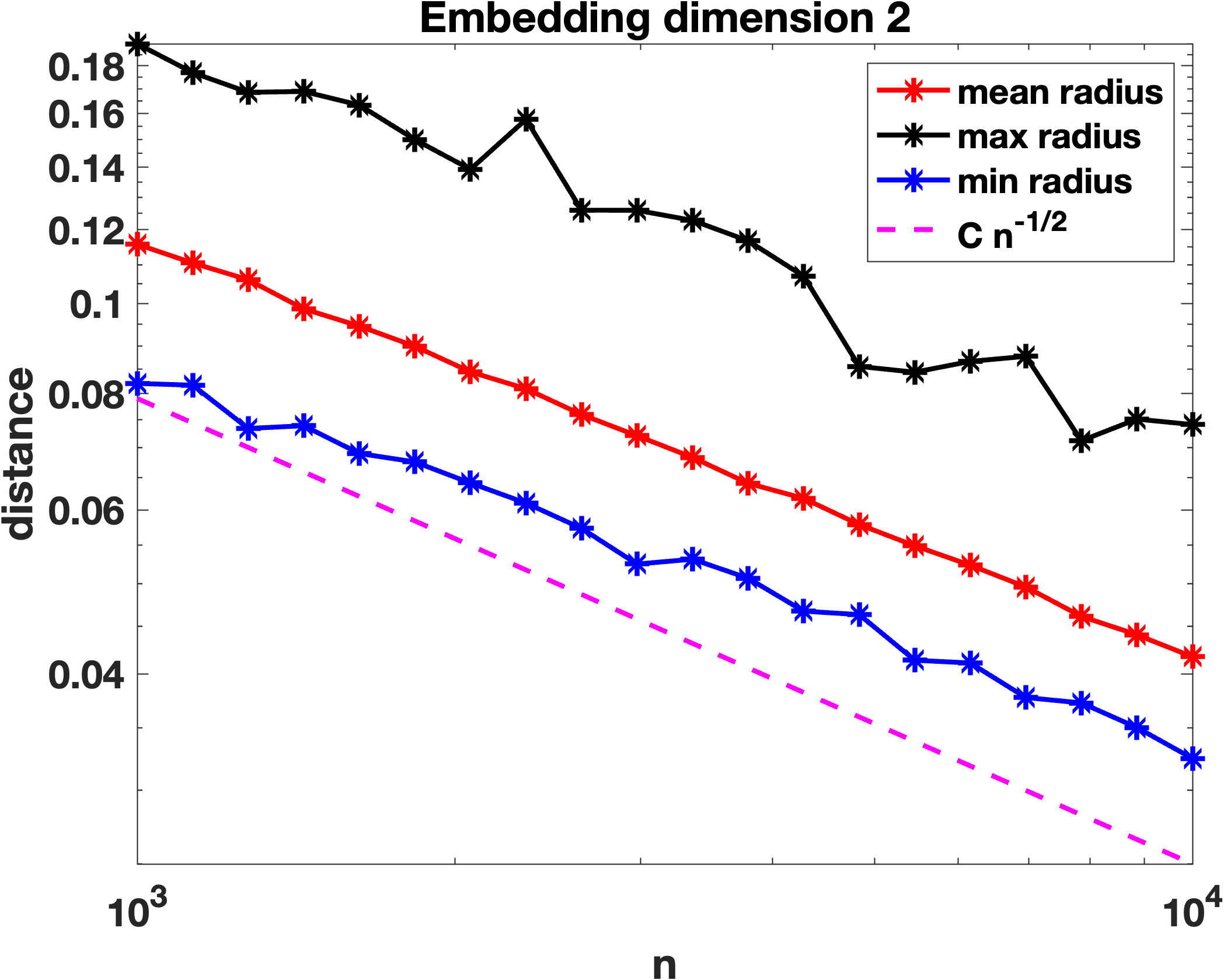
Figure 2: Euclidean distance at which geometric random hypergraph becomes connected. Here we have $0.8n$ nodes and $0.2n$ hyperedge centres in $\mathbb{R}^{2}$, for values of $n$ between $10^{3}$ and $10^{4}$. The plots show the mean, maximum and minimum value of this distance over $500$ independent trials. A reference slope corresponding to $Cn^{-{\scriptstyle{{\frac{1}{2}}}}}$ is shown. Axes are logarithmically scaled.

Figures 3 and 4 repeat these computations with points embedded into $\mathbb{R}^{4}$ and $\mathbb{R}^{10}$, respectively. We see that the behaviour remains remains consistent with a decay roughly proportional to, and perhaps slightly slower than, $n^{-1/d}$ for dimension $d$.

In the next section we formalize our definition of a random geometric hypergraph and establish an upper bound on the radius decay rate for connectivity that agrees with $n^{-1/d}$, up to $\log$-dependent factors (which of course would be extremely difficult to pin down in computational experiments). We also note for comparison that a threshold of the form $(\log(n)/n)^{1/d}$ has previously arisen in the study of random geometric graphs, [2, 23].

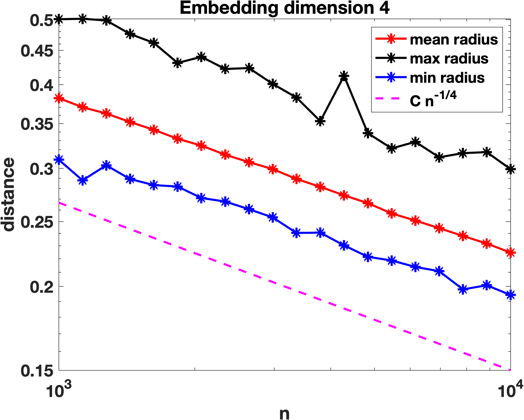
Figure 3: As for Figure 2 with nodes embedded in $\mathbb{R}^{4}$ and a reference slope corresponding to $Cn^{-{\scriptstyle{{\frac{1}{4}}}}}$.

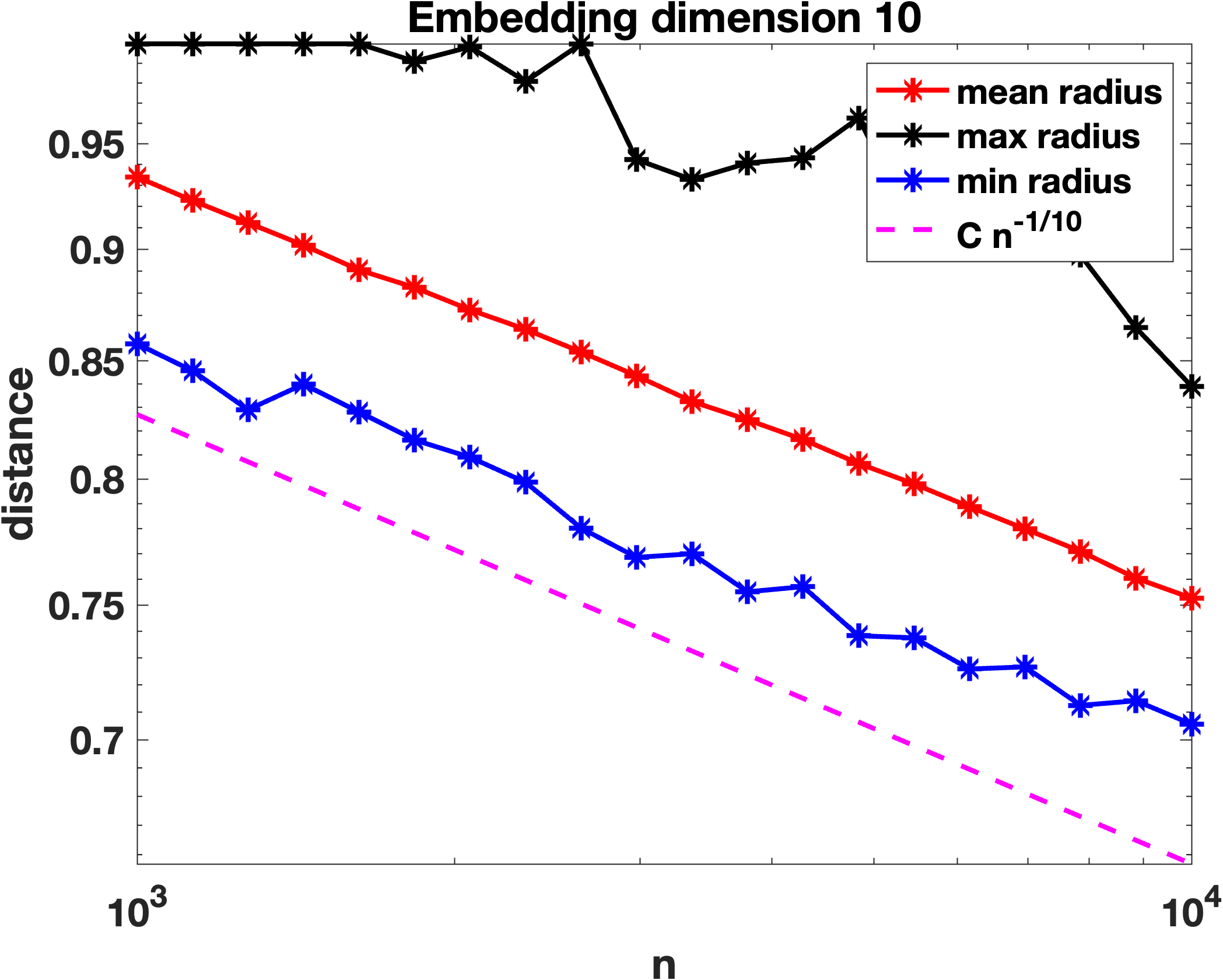
Figure 4: As for Figure 2 with nodes embedded in $\mathbb{R}^{10}$ and a reference slope corresponding to $Cn^{-{\scriptstyle{{\frac{1}{10}}}}}$.

In related work, we note that Barthelemy [3] proposed and studied a wide class of random hypergraph models, including examples where nodes are embedded in space and connections arise via a distance measure. That approach to defining a random geometric hypergraph differs from ours by assuming that the number of hyperedges is given and by considering a process where new nodes are added to the network, with new connections arising based in the current hyperedge memberships ([3, Figure 6]).

3 Connectivity Analysis

We now give a formal definition of a random geometric hypergraph and show that under reasonable conditions a thresholding radius of order $(\log(n)/n)^{1/d}$ ensures connectivity, asymptotically.

Let $D$ be a bounded Euclidean domain in $\mathbb{R}^{d}$, such that $D$ has Lipschitz boundary. Given $n\in\mathbb{N}$, we let $\mathcal{P}_{n}$ be a Poisson point process sampled from $D$ with respect to some continuous and bounded distribution $f$, such that $f>0$ everywhere on $D$. We use $|\cdot|$ to denote the Euclidean norm. Let $n\in\mathbb{N}$, and let $n_{1}$ be the expeted number of nodes and $n_{2}$ be the expected number of hyperedges, chosen such that $n=n_{1}+n_{2}$. Let $r_{n}$ be a function of $n$, tending to $0$ as $n\to\infty$.

Definition 1.

Let $G(n_{1},n_{2},r_{n})$ be the probability space on the set of geometric hypergraphs, where the random nodes are chosen as a Poisson point process $\mathcal{P}_{n_{1}}$ in $D$ sampled with respect to $f$, the random hyperedges are induced by another Poisson point process $\mathcal{P}_{n_{2}}$ in $D$ sampled with respect to $f$, and where, using bipartite graph-hypergraph equivalance, a node $x\in\mathcal{P}_{n_{1}}$ and a hyperedge $y\in\mathcal{P}_{n_{2}}$ are connected by an edge if $\mathinner{\!\left\lvert x-y\right\rvert}<r_{n}$.

Suppose that the expected number of nodes $n_{1}$ and of hyperedges $n_{2}$ satisfy

$$\frac{n_{1}}{n_{2}}=\Theta(1).$$

Equivalently, this means that $n_{1}$ and $n_{2}$ as functions of $n$ satisfy

$$n_{1}=\Theta(n),\quad n_{2}=\Theta(n).$$

Let $K>0$ be the smallest constant such that for all $n\in\mathbb{N}$,

$$n_{1}\geq\frac{1}{K}n\quad\text{ and }\quad n_{2}\geq\frac{1}{K}n.$$ (1)

Partition $\mathbb{R}^{d}$ into a grid of cubes $\{C_{i,n}\}_{i}$ of width $\gamma r_{n}$, where $r_{n}=o(1)$ and $\gamma>0$ is to be determined. Let $S_{n}\mathrel{\mathop{\ordinarycolon}}=\{i\ |\ C_{i,n}\subset D\}$, and for each $i\in S_{n}$, let $\mathcal{I}(i,n)\mathrel{\mathop{\ordinarycolon}}=\{j\not\in S_{n}\ |\ C_{j,n}\text{ is adjacent to }C_{i,n}\},$ and let

$$Q_{i,n}\mathrel{\mathop{\ordinarycolon}}=\cup_{j\in\mathcal{I}(i,n)}(C_{j,n}\cap D).$$

Since $D$ has a Lipschitz boundary, by compactness there exists $C>0$ depending on $D$ and $d$ (but not on $\gamma$), such that we can choose $n_{0}\in\mathbb{N}$ sufficiently large such that for all $n\geq n_{0}$ and all $i\in S_{n}$

$$\forall\ x,y\in Q_{i,n},\ \mathinner{\!\left\lvert x-y\right\rvert}<C\gamma r_{n}.$$

We then choose $\gamma\mathrel{\mathop{\ordinarycolon}}=\frac{1}{C},$ so that for all $i\in S_{n}$,

$$\forall\ x,y\in Q_{i,n},\ \mathinner{\!\left\lvert x-y\right\rvert}<r_{n}.$$ (2)

Note also that we have $\nu(Q_{i,n})\geq\nu(C_{i,n})\geq f_{\min}\gamma^{d}r_{n}^{d}=\frac{f_{\min}}{C^{d}}r_{n}^{d},$ where $f_{\min}\mathrel{\mathop{\ordinarycolon}}=\min\{f(x)\ |\ x\in\Omega\}.$

Lemma 3.1 (Asymptotic coverage).

Suppose that $m$ as a function of $n$ satisfies, for all $n\in\mathbb{N}$,

$$m\geq\frac{1}{K}n,$$

and suppose that $r_{n}$ satisfies

$$n\frac{f_{\min}}{KC^{d}}r_{n}^{d}\geq\log n-\log\log n+w(n),$$ (3)

where $w(n)\to\infty$ arbitrarily slowly as $n\to\infty$. With probability tending to $1$ as $n\to\infty$, for all $i\in S_{n}$

$$\mathcal{P}_{m}\cap Q_{i,n}\neq\emptyset.$$

Proof.

It suffices to show that the RHS in

$$\mathbb{P}(\exists\ i\in S_{n},\mathcal{P}_{m}(Q_{i,n})=0)\leq\sum_{i\in S_{n}}\mathbb{P}(\mathcal{P}_{n}(Q_{i,n})=0)$$

tends to $0$ as $n\to\infty$.

Since $\mathcal{P}_{m}$ is a homogeneous Poisson point process, we have, using (3), for all $i\in S_{n}$

$$\mathbb{P}(\mathcal{P}_{m}(Q_{i,n})=0)=\exp(-m\nu(Q_{i,n}))\leq\exp\left(-n\frac{f_{\min}}{KC^{d}}r_{n}^{d}\right)\leq n^{-1}(\log n)e^{-w(n)},$$

and by the pigeonhole principle, $\mathinner{\!\left\lvert S_{n}\right\rvert}\lesssim(\gamma r_{n})^{-d}\lesssim n(\log n)^{-1}$. Hence

$$\mathbb{P}(\exists\ i\in S_{n},\mathcal{P}_{n}(Q_{i,n})=0) \lesssim e^{-w(n)}.$$

∎

Note that with our choice of $\gamma$, we have

$$\{\forall\ i\in S_{n}\ |\ \mathcal{P}_{m}\cap Q_{i,n}\neq\emptyset\}\subset\{D\subset\cup_{x\in\mathcal{P}_{m}}B(x,r_{n})\}.$$

Hence Lemma 3.1 gives us a lower bound estimate on the decay of $r_{n}$ as a function of $n$, to ensure that the balls centered at the points of $\mathcal{P}_{m}$ and of radius $r_{n}$, tend to form a covering of the domain $D$ as $n\to\infty$. This is an asymptotic result.

From a practical point of view, it is more useful to have a non-asymptotic version of Lemma 3.1, even if we must increase slightly the constraint on the decay of $r_{n}$. This is the object of Lemma 3.2.

Lemma 3.2 (Non-asymptotic coverage).

Suppose that $m$ as a function of $n$ satisfies, for all $n\in\mathbb{N}$,

$$m\geq\frac{1}{K}n,$$

and suppose this time that $r_{n}$ satisfies

$$n\frac{f_{\min}}{KC^{d}}r_{n}^{d}\geq 2\log n+\epsilon\log\log n,$$ (4)

for some fixed $\epsilon>0$, then a.s., there exists $N\in\mathbb{N}$ such that for all $n\geq N$ and all $i\in S_{n}$

$$\mathcal{P}_{m}\cap Q_{i,n}\neq\emptyset.$$

Proof.

A proof proceeds similarly to that of Lemma 3.1, but the different constraint on $r_{n}$ yields instead

$$\mathbb{P}(\exists\ i\in S_{n},\mathcal{P}_{m}(Q_{i,n})=0)\lesssim\frac{1}{n(\log n)^{1+\epsilon}},$$

and the required result then follows by the Borel-Cantelli lemma, since then, the series

$$\sum_{n=0}^{N}\ \mathbb{P}(\exists\ i\in S_{n},\mathcal{P}_{m}(Q_{i,n})=0)$$

converges as $N\to\infty$. ∎

We believe that the lower bound condition on the decay of $r_{n}$ found in Lemma 3.1 is sharp, and that the lower bound condition in Lemma 3.2 is close to being sharp. In Theorem 3.3 we apply Lemmas 3.1 and 3.2 to obtain a sufficient lower bound condition on $r_{n}$ for the connectivity of random geometric hypergraphs, with an extra factor of $2$. We suspect that this factor could be reduced by more sophisticated analysis.

Theorem 3.3.

For every $n\in\mathbb{N}$, let $(n_{1},n_{2})\in\mathbb{N}^{2}$ satisfy (1) and $n=n_{1}+n_{2}$.

• If $r_{n}$ satisfies (3), then with probability tending to $1$ as $n\to\infty$, the random graph $G(n_{1},n_{2},2r_{n})$ is connected.
  

• If $r_{n}$ satisfies (4), then a.s. there exists $N\in\mathbb{N}$, such that for all $n\geq N$, the random geometric bipartite graph $G(n_{1},n_{2},2r_{n})$ is connected.

Proof.

The result is a consequence of Lemmas 3.1 and 3.2 and the triangle inequality.

Suppose that $n\in\mathbb{N}$ is such that for all $i\in S_{n}$

$$\mathcal{P}_{n_{1}}\cap Q_{i,n}\neq\emptyset\quad\text{ and }\quad\mathcal{P}_{n_{2}}\cap Q_{i,n}\neq\emptyset.$$ (5)

Given two points $x,y\in\mathcal{P}_{n_{1}}$, we can find a path of adjacent cubes from $\mathcal{Q}_{n}$, such that the first cube contains $x$ and the last cube contains $y$. From (2) and the triangle inequality, the distance between a point in one cube and another point in an adjacent cube is at most $2r_{n}$. Since for each cube in the path we can find a point from $\mathcal{P}_{n_{1}}$ and a point from $\mathcal{P}_{n_{2}}$, we can then form a path of edges of length at most $2r_{n}$ from $x$ to $y$, alternating between points in $\mathcal{P}_{n_{1}}$ and points in $\mathcal{P}_{n_{2}}$, and such a path is then a path in $\mathcal{G}(n_{1},n_{2},2r_{n}).$

This shows connectivity of the graph for all $n$ satisfying condition (5).

This condition is true with probability tending to $1$ as $n\to\infty$, if we assume that $r_{n}$ satisfies (3), using Lemma 3.1 with $n_{1}$ and $n_{2}$ instead of $m$, giving us the first part of the theorem.

Using Lemma 3.2 with $n_{1}$ and $n_{2}$ instead of $m$, if $r_{n}$ satisfies (4), there exists $N\in\mathbb{N}$ such that (5) is true for all $n\geq N$, giving us the second part of the theorem. ∎

4 Discussion

There are a number of promising avenues for further work in this area. From a theoretical perspective, it would be of interest to derive useful upper bounds or indeed sharp expressions for the exact connectivity radius threshold associated with this class of random geometric hypergraphs. More general hypergraph models could also be developed and studied, for example using a softer version of the distance cut-off that has been considered in the graph setting [9, 25].

From a more practical viewpoint, the related inverse problem is both challenging and potentially useful: given a data set that corresponds to a hypergraph, for the model considered here what is the best choice of (a) embedding dimension, (b) node locations, and (c) hypergraph centre locations? A similar question was addressed in [15] for a different generative random hypergraph model based on the assumption that nodes are located in a latent space and hyperedges arise preferentially between nearby nodes (without the concept of hyperedge centres). This challenge also leads into the model selection question: given a data set and selection of hypergraph models, which one best describes the data, and what insights arise?

Acknowledgement Both authors were supported by Engineering and Physical Sciences Research Council grant EP/P020720/1. The second author was also supported by Engineering and Physical Sciences Research Council grant EP/W011093/1.

References

- [1] U. Alvarez-Rodriguez, F. Battiston, G. F. de Arruda, Y. Moreno, M. Perc, and V. Latora. Evolutionary dynamics of higher-order interactions in social networks. Nat. Hum. Behav., 2021.
- [2] Martin J.B. Appel and Ralph P. Russo. The connectivity of a graph on uniform points on . Statistics and Probability Letters, 60(4):351–357, 2002.
- [3] Marc Barthelemy. Class of models for random hypergraphs. Phys. Rev. E, 106:064310, 2022.
- [4] Federico Battiston, Giulia Cencetti, Iacopo Iacopini, Vito Latora, Maxime Lucas, Alice Patania, Jean-Gabriel Young, and Giovanni Petri. Networks beyond pairwise interactions: Structure and dynamics. Physics Reports, 874:1–92, 2020.
- [5] Austin R Benson, David F Gleich, and Jure Leskovec. Higher-order organization of complex networks. Science, 353(6295):163–166, 2016.
- [6] Ginestra Bianconi. Higher order networks : An introduction to simplicial complexes. Cambridge University Press, 2021.
- [7] Ágnes Bodó, Gyula Katona, and Péter Simon. SIS epidemic propagation on hypergraphs. Bulletin of Mathematical Biology, 78(4):713–735, 2016.
- [8] Philip S. Chodrow, Nate Veldt, and Austin R. Benson. Generative hypergraph clustering: From blockmodels to modularity. Science Advances, 7(28):eabh1303, 2021.
- [9] C. P. Dettmann. Isolation and connectivity in random geometric graphs with self-similar intensity measures. J. Stat Phys., pages 679–700, 2018.
- [10] Quentin Duchemin and Yohann De Castro. Random geometric graph: Some recent developments and perspectives. In Radosław Adamczak, Nathael Gozlan, Karim Lounici, and Mokshay Madiman, editors, High Dimensional Probability IX, pages 347–392. Springer International Publishing, 2023.
- [11] Martin Dyer, Catherine Greenhill, Pieter Kleer, James Ross, and Leen Stougie. Sampling hypergraphs with given degrees. 344(11), 2021.
- [12] Ernesto Estrada and Juan A. Rodríguez-Velázquez. Subgraph centrality and clustering in complex hyper-networks. Physica A: Statistical Mechanics and its Applications, 364(C):581–594, 2006.
- [13] Debarghya Ghoshdastidar and Ambedkar Dukkipati. Consistency of spectral hypergraph partitioning under planted partition model. The Annals of Statistics, 45(1):289 – 315, 2017.
- [14] E. N. Gilbert. Random plane networks. Journal of the Society for Industrial and Applied Mathematics, 9:533–543, 1961.
- [15] X. Gong, D. J. Higham, and K. Zygalakis. Generative hypergraph models and spectral embedding. Sci. Rep., 13, 2023.
- [16] Peter Grindrod. Range-dependent random graphs and their application to modeling large small-world proteome datasets. Physical Review. E, 66(6):066702/7–066702, 2002.
- [17] D. J. Higham, M. Rašajski, and N. Przulj. Fitting a geometric graph to a protein-protein interaction network. Bioinformatics, 24:1093–1099, 2008.
- [18] Desmond J Higham and Henry-Louis De Kergorlay. Epidemics on hypergraphs: Spectral thresholds for extinction. Proceedings of the Royal Society A, 477(2252):20210232, 2021.
- [19] Desmond John Higham and Henry-Louis de Kergorlay. Mean field analysis of hypergraph contagion models. SIAM Journal on Applied Mathematics, 82(6):1987–2007, 2022.
- [20] Nicholas W. Landry and Juan G. Restrepo. The effect of heterogeneity on hypergraph contagion models. Chaos, 30(10), 2020.
- [21] Leonie Neuhäuser, Michael Scholkemper, Francesco Tudisco, and Michael T. Schaub. Learning the effective order of a hypergraph dynamical system. arXiv 2306.01813, 2023.
- [22] Massimo Ostilli and Ginestra Bianconi. Statistical mechanics of random geometric graphs: Geometry-induced first-order phase transition. Phys. Rev. E, 91:042136, 2015.
- [23] Mathew D. Penrose. The longest edge of the random minimal spanning tree. The Annals of Applied Probability, 7(2):340–361, 1997.
- [24] Mathew D. Penrose. Random Geometric Graphs. Oxford University Press, 2003.
- [25] Mathew D. Penrose. Connectivity of soft random geometric graphs. The Annals of Applied Probability, 26(2):986 – 1028, 2016.
- [26] N. Przulj and D. J. Higham. Modelling protein-protein interaction networks via a stickiness index. J. Royal Society Interface, pages 711–716, 2006.
- [27] Bernhard Schölkopf, John Platt, and Thomas Hofmann. Learning with hypergraphs: Clustering, classification, and embedding. In Advances in Neural Information Processing Systems 19: Proceedings of the 2006 Conference, pages 1601–1608, 2007.
- [28] Leo Torres, Ann S. Blevins, Danielle S. Bassett, and Tina Eliassi-Rad. The why, how, and when of representations for complex systems. SIAM Review, 63:435–485, 2021.
- [29] Francesco Tudisco and Desmond J. Higham. Node and edge nonlinear eigenvector centrality for hypergraphs. Communications Physics, 4(1):201, 2021.
- [30] Francesco Tudisco and Desmond J Higham. Core-periphery detection in hypergraphs. arXiv preprint arXiv:2202.12769, 2022.
- [31] Z. Xie, Z. Ouyang, Q. Liu, and J. Li. A geometric graph model for citation networks of exponentially growing scientific papers. pages 167–175, 2016.
- [32] Naganand Yadati, Vikram Nitin, Madhav Nimishakavi, Prateek Yadav, Anand Louis, and Partha Talukdar. Nhp: Neural hypergraph link prediction. In Proceedings of the 29th ACM International Conference on Information & Knowledge Management, pages 1705–1714, 2020.
- [33] Seeun Yoon, Hyungseok Song, Kijung Shin, and Yung Yi. How much and when do we need higher-order information in hypergraphs? a case study on hyperedge prediction. In Proceedings of The Web Conference 2020, pages 2627–2633, 2020.