Model-based Subsampling for Knowledge Graph Completion

Abstract

Subsampling is effective in Knowledge Graph Embedding (KGE) for reducing overfitting caused by the sparsity in Knowledge Graph (KG) datasets. However, current subsampling approaches consider only frequencies of queries that consist of entities and their relations. Thus, the existing subsampling potentially underestimates the appearance probabilities of infrequent queries even if the frequencies of their entities or relations are high. To address this problem, we propose Model-based Subsampling (MBS) and Mixed Subsampling (MIX) to estimate their appearance probabilities through predictions of KGE models. Evaluation results on datasets FB15k-237, WN18RR, and YAGO3-10 showed that our proposed subsampling methods actually improved the KG completion performances for popular KGE models, RotatE, TransE, HAKE, ComplEx, and DistMult.

1 Introduction

A Knowledge Graph (KG) is a graph that contains entities and their relations as links. KGs are important resources for various NLP tasks, such as dialogue Moon et al. (2019), question-answering Lukovnikov et al. (2017), and natural language generation Guan et al. (2019), etc. However, covering all relations of entities in a KG by humans takes a lot of costs. Knowledge Graph Completion (KGC) tries to solve this problem by automatically completing lacking relations based on the observed ones. Letting $e_{i}$ and $e_{k}$ be entities, and $r_{j}$ be their relation, KGC models predict the existence of a link $(e_{i},r_{j},e_{k})$ by filling the $?$ in the possible links $(e_{i},r_{j},?)$ and $(?,r_{j},e_{k})$, where $(e_{i},r_{j})$ and $(r_{j},e_{k})$ are called queries, and the $?$ are the corresponding answers.

Figure 1: The averaged KGC performance (MRR) of KGE modelswith and without subsampling on FB15k-237, WN18RR, and YAGO3-10.

Currently, Knowledge Graph Embedding (KGE) is a dominant approach for KGC. KGE models represent entities and their relations as continuous vectors. Since the number of these vectors proportionally increases to the number of links in a KG, KGE commonly relies on Negative Sampling (NS) to reduce the computational cost in training. In NS, a KGE model learns a KG by discriminating between true links and false links created by sampling links in the KG. While NS can reduce the computational cost, it has the problem that the sampled links also reflect the bias of the original KG.

As a solution, Sun et al. (2019) introduce subsampling Mikolov et al. (2013) into NS for KGE. In this usage, subsampling is a method of mitigating bias in a KG by discounting the appearance frequencies of links with high-frequent queries and reserving the appearance frequencies for links with low-frequent queries. Figure 2 shows the effectiveness of using subsampling. From this figure, we can understand that KGE models cannot perform well without subsampling on commonly used datasets such as FB15k-237 Toutanova and Chen (2015), WN18RR Dettmers et al. (2018), and YAGO3-10 Dettmers et al. (2018). Furthermore, the improved MRR on FB15k-237, which has more sparse relations than the other datasets, indicates that subsampling actually works on the sparse dataset.

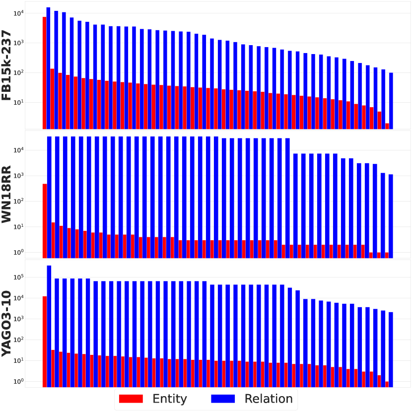
Figure 2: Frequencies of entities and relations included in each query that appeared only once in training data of FB15k-237, WN18RR, and YAGO3-10.

However, the current subsampling approaches in KGE Sun et al. (2019); Kamigaito and Hayashi (2022a) only consider the frequencies of queries. Thus, these approaches potentially underestimate the appearance probabilities of infrequent queries when the frequencies of their entities or relations are high. Figure 4 shows the frequencies of entities and relations included in each query that appeared only once in training data. From the statistics, we can find that the current count-based subsampling (CBS) does not effectively use frequencies of entities and relations in infrequent queries, although these have sufficient frequencies.

To deal with this problem, we propose Model-based Subsampling (MBS) that can handle such infrequent queries by estimating their appearance probabilities through predictions from KGE models in subsampling. Since the observed frequency in training data does not restrict the estimated frequencies of MBS different from CBS, we can expect the improvement of KGC performance using MBS. In addition, we also propose Mixed Subsampling (MIX), which uses the frequencies of both CBS and MBS to boost their advantage by reducing their disadvantages.

In our evaluation on FB15k-237, WN18RR, and YAGO3-10 datasets, we adopted our MBS and MIX to the popularly used KGE models RotatE Sun et al. (2019), TransE Bordes et al. (2013), HAKE Zhang et al. (2019), ComplEx Trouillon et al. (2016), and DistMult Yang et al. (2015). The evaluation results showed that MBS and MIX improved MRR, H@1, H@3, and H@10 from Count-based Subsampling (CBS) in each setting.

2 Subsampling in KGE

2.1 Problem Definitions and Notations

We denote a link of a KG in the triplet format $(h,r,t)$. $h$ is the head entity, $t$ is the tail entity, and $r$ is the relation of the head and tail entity. In a classic KG completion task, we input the query $(h,r,?)$ or $(?,r,t)$, and output the predicted head or tail entity corresponding to $?$ as the answer. More formally, let us denote the input query as $x$ and its answer as $y$, hereafter. A score function $s_{\mathbf{\theta}}(x,y)$ predicts $p_{\mathbf{\theta}}(y|x)$, a probability for a given query $x$ linked to an answer $y$ based on a model $\mathbf{\theta}$. In general, we train $\mathbf{\theta}$ by predicting $p_{\mathbf{\theta}}(y|x)$ on $|D|$ number of links, where $D=\{(x_{1},y_{1}),\cdots,(x_{|D|},y_{|D|})\}$ is a set of observables that follow $p_{d}(x,y)$.

2.2 Negative Sampling in KGE

Since calculating all possible $y$ for given $x$ is computationally inefficient, NS loss is commonly used for training KGE models. The NS loss in KGE, $\ell_{kge}(\mathbf{\theta})$ is represented as follows:

$$\ell_{kge}(\mathbf{\theta})$$

$$= -\frac{1}{|D|}\sum_{(x,y)\in D}\Bigl{[}\log(\sigma(s_{\mathbf{\theta}}(x,y)+\gamma))$$

$$+\frac{1}{\nu}\sum_{y_{i}\sim p_{n}(y_{i}|x)}^{\nu}\log(\sigma(-s_{\mathbf{\theta}}(x,y_{i})-\gamma))\Bigr{]},$$ (1)

where $\sigma$ is a sigmoid function, $p_{n}(y_{i}|x)$ is a noise distribution describing negative samples, $\nu$ is a number of negative samples per positive sample $(x,y)$, $\gamma$ is a margin term to adjust the value range of the score function. $p_{n}(y_{i}|x)$ has a role of adjusting the frequency of $y_{i}$ Kamigaito and Hayashi (2021).

2.3 Negative Sampling with Subsampling

Subsampling Mikolov et al. (2013) is a method to reduce the bias of training data by discounting high-frequent instances. Kamigaito and Hayashi (2022a) show a general formulation to cover currently proposed subsampling approaches in the NS loss for KGE by altering two terms $A_{cbs}$ and $B_{cbs}$. In that form, the NS loss in KGE with subsampling, $\ell_{cbs}(\mathbf{\theta})$ is represented as follows:

$$\ell_{cbs}(\mathbf{\theta})$$

$$= -\frac{1}{|D|}\sum_{(x,y)\in D}\Bigl{[}A_{cbs}\log(\sigma(s_{\mathbf{\theta}}(x,y)+\gamma))$$

$$+\frac{1}{\nu}\sum_{y_{i}\sim p_{n}(y_{i}|x)}^{\nu}B_{cbs}\log(\sigma(-s_{\mathbf{\theta}}(x,y_{i})-\gamma))\Bigr{]},$$ (2)

where $A_{cbs}$ adjusts the frequency of a true link $(x,y)$, and $B_{cbs}$ adjusts the query $x$ to adjust the frequency of a false link $(x,y_{i})$.

Method	$A_{cbs}$	$B_{cbs}$
Base	$\frac{\frac{1}{\sqrt{\#(x,y)}}|D|}{\sum_{(x^{\prime},y^{\prime})\in D}\frac{1}{\sqrt{\#(x^{\prime},y^{\prime})}}}$	$\frac{\frac{1}{\sqrt{\#(x,y)}}|D|}{\sum_{(x^{\prime},y^{\prime})\in D}\frac{1}{\sqrt{\#(x^{\prime},y^{\prime})}}}$
Freq	$\frac{\frac{1}{\sqrt{\#(x,y)}}|D|}{\sum_{(x^{\prime},y^{\prime})\in D}\frac{1}{\sqrt{\#(x^{\prime},y^{\prime})}}}$	$\frac{\frac{1}{\sqrt{\#x}}|D|}{\sum_{x^{\prime}\in D}{\frac{1}{\sqrt{\#x^{\prime}}}}}$
Uniq	$\frac{\frac{1}{\sqrt{\#x}}|D|}{\sum_{x^{\prime}\in D}{\frac{1}{\sqrt{\#x^{\prime}}}}}$	$\frac{\frac{1}{\sqrt{\#x}}|D|}{\sum_{x^{\prime}\in D}{\frac{1}{\sqrt{\#x^{\prime}}}}}$

Table 1: Currently proposed count-based subsampling methods in KGE and their corresponding terms on $A_{cbs}$ and $B_{cbs}$.

Table 1 lists the currently proposed subsampling approaches which are the original subsampling for word2vec (Mikolov et al., 2013) in KGE of Sun et al. (2019) (Base), frequency-based subsampling of Kamigaito and Hayashi (2022a) (Freq), and unique-based subsampling of Kamigaito and Hayashi (2022a) (Uniq) Kamigaito and Hayashi (2022b). Here, $\#$ denotes frequency, $\#(x,y)$ represents the frequency of $(x,y)$.

Since frequency for each link $(x,y)$ is at most one in KG, the previous approaches use the following back-off approximation (Katz, 1987):

$$\#(x,y)\approx\frac{\#(h_{i},r_{j})\!+\#(r_{j},t_{k})}{2},$$ (3)

where $(x,y)$ corresponds to the link $(h_{i},r_{j},t_{k})$, and $(h_{i},r_{j})$ and $(r_{j},t_{k})$ are the queries. Due to their heavily relying on counted frequency information of queries, we call the above conventional subsampling method Count-based Subsamping (CBS), hereafter.

3 Proposed Methods

As shown in Equation (3), CBS approximates the frequency of a link $\#(x,y)$ by combining the counted frequencies of entity-relation pairs. Thus, CBS cannot estimate $\#(x,y)$ well when at least one pair’s frequency is low in the approximation. This kind of situation is caused by the sparseness problem in the KG datasets. To deal with this sparseness problem, we propose Model-based Subsampling method (MBS) and Mixed Subsampling method (MIX) as described in the following subsections.

3.1 Model-based Subsampling (MBS)

To avoid the problem caused by low-frequent entity-relation pairs, our MBS uses the estimated probabilities from a trained model $\mathbf{\theta}^{\prime}$ to calculate frequencies for each triplet and query. By using $\mathbf{\theta}^{\prime}$, the NS loss in KGE with MBS is represented as follows:

$$\ell_{mbs}(\mathbf{\theta};\mathbf{\theta}^{\prime})$$

$$= -\frac{1}{|D|}\sum_{(x,y)\in D}\Bigl{[}A_{mbs}(\mathbf{\theta}^{\prime})\log(\sigma(s_{\mathbf{\theta}}(x,y)+\gamma))$$

$$+\frac{1}{\nu}\!\!\!\!\!\!\sum_{y_{i}\sim p_{n}(y_{i}|x)}^{\nu}\!\!\!\!\!\!B_{mbs}(\mathbf{\theta}^{\prime})\log(\sigma(-s_{\mathbf{\theta}}(x,y_{i})-\gamma))\Bigr{]},$$ (4)

Here, corresponding to each method in Table 4, $A_{mbs}(\mathbf{\theta}^{\prime})$ and $B_{mbs}(\mathbf{\theta}^{\prime})$ are further represented as follows:

$$A_{mbs}(\mathbf{\theta}^{\prime}) =\left\{\begin{array}[]{*2{>{\displaystyle}l}}\frac{\#(x,y)_{mbs}^{-\alpha}|D|}{\sum_{(x^{\prime},y^{\prime})\in D}\#(x^{\prime},y^{\prime})_{mbs}^{-\alpha}}&\mathrm{(Base)}\\ \frac{\#(x,y)_{mbs}^{-\alpha}|D|}{\sum_{(x^{\prime},y^{\prime})\in D}\#(x^{\prime},y^{\prime})_{mbs}^{-\alpha}}&\mathrm{(Freq)}\\ \frac{\#x_{mbs}^{-\alpha}|D|}{\sum_{x^{\prime}_{mbs}\in D}{{\#x^{\prime}}_{mbs}^{-\alpha}}}&\mathrm{(Uniq)}\end{array}\right.$$ (8)

$$B_{mbs}(\mathbf{\theta}^{\prime}) =\left\{\begin{array}[]{*2{>{\displaystyle}l}}\frac{\#(x,y)_{mbs}^{-\alpha}|D|}{\sum_{(x^{\prime},y^{\prime})\in D}\#(x^{\prime},y^{\prime})_{mbs}^{-\alpha}}&\mathrm{(Base)}\\ \frac{\#x_{mbs}^{-\alpha}|D|}{\sum_{x^{\prime}_{mbs}\in D}{\#x^{\prime}}_{mbs}^{-\alpha}}&\mathrm{(Freq)}\\ \frac{\#x_{mbs}^{-\alpha}|D|}{\sum_{x^{\prime}_{mbs}\in D}{\#x^{\prime}}_{mbs}^{-\alpha}}&\mathrm{(Uniq)}\end{array}\right.$$ (12)

where $\alpha$ is a temperature term to adjust the distribution on $A_{mbs}(\mathbf{\theta}^{\prime})$ and $B_{mbs}(\mathbf{\theta}^{\prime})$. The frequencies $\#(x,y)_{mbs}$ and $\#x_{mbs}$, estimated by using $score_{\mathbf{\theta}^{\prime}}(x,y)$ are calculated as follows:

$$\#(x,y)_{mbs} =|D|p_{\mathbf{\theta}^{\prime}}(x,y),$$ (13)

$$\#x_{mbs} =|D|\textstyle\sum_{y_{i}\in D}p_{\mathbf{\theta}^{\prime}}(x,y_{i}),$$ (14)

$$p_{\mathbf{\theta}^{\prime}}(x,y) =\frac{e^{score_{\mathbf{\theta}^{\prime}}(x,y)}}{\sum_{(x^{\prime},y^{\prime})\in D}e^{score_{\mathbf{\theta}^{\prime}}(x^{\prime},y^{\prime})}}.$$ (15)

Hereafter, we refer to a model pre-trained for MBS as a sub-model. Different from the counted frequencies in Eq. (3), $score_{\mathbf{\theta}^{\prime}}(x,y)$ in Eq. (15) estimates them by sub-model inference regardless of their actual frequencies. Hence, we can expect MBS to deal with the sparseness problem in CBS. However, the ability of MBS depends on the sub-model, and we investigated the performance through our evaluations (§4).

3.2 Mixed Subsampling (MIX)

As discussed in language modeling context (Neubig and Dyer, 2016), count-based and model-based frequencies have different strengths and weaknesses. To boost the advantages of CBS and MBS by mitigating their disadvantages, MIX uses a mixture of the distribution as follows:

$$\ell_{mix}(\mathbf{\theta};\mathbf{\theta}^{\prime})$$

$$= -\frac{1}{|D|}\sum_{(x,y)\in D}\Bigl{[}A_{mix}(\mathbf{\theta}^{\prime})\log(\sigma(s_{\mathbf{\theta}}(x,y)+\gamma))$$

$$+\frac{1}{\nu}\!\!\!\!\!\!\sum_{y_{i}\sim p_{n}(y_{i}|x)}^{\nu}\!\!\!\!\!\!B_{mix}(\mathbf{\theta}^{\prime})\log(\sigma(-s_{\mathbf{\theta}}(x,y_{i})-\gamma))\Bigr{]},$$ (16)

where $A_{mix}(\mathbf{\theta}^{\prime})$ is a mixture of $A_{cbs}$ in Eq. (2) and $A_{mbs}(\mathbf{\theta}^{\prime})$ in Eq. (4), and $B_{mix}(\mathbf{\theta}^{\prime})$ is also a mixture of $B_{cbs}$ in Eq. (2) and $B_{mbs}(\mathbf{\theta}^{\prime})$ Eq. (4) as follows:

$$A_{mix}(\mathbf{\theta}^{\prime})=\lambda A_{mbs}(\mathbf{\theta}^{\prime})+(1-\lambda)A_{cbs}$$ (17)

$$B_{mix}(\mathbf{\theta}^{\prime})=\lambda B_{mbs}(\mathbf{\theta}^{\prime})+(1-\lambda)B_{cbs}$$ (18)

where $\lambda$ is a hyper-parameter to adjust the ratio of MBS and CBS. Note that MIX can be interpreted as a kind of multi-task learning.

4 Evaluation and Analysis

4.1 Settings

Datasets

We used the three commonly used datasets, FB15k-237, WN18RR, and YAGO3-10, for the evaluation. Table 2 shows the statistics for each dataset. Unlike FB15k-237 and WN18RR, the dataset of YAGO3-10 only includes entities that have at least 10 relations and alleviates the sparseness problem of KGs. Thus, we can investigate the effectiveness of MBS and MIX in the sparseness problem by comparing performances on these datasets.

Methods

We compared five popular KGE models RotatE, TransE, HAKE, ComplEx, and DistMult with utilizing subsampling methods Base, Freq, and Uniq based on the loss of CBS (§2.3) and our MBS (§3.1) and MIX (§3.2). Additionally, we conducted experiments with no subsampling (None) to investigate the efficacy of the subsampling method. In YAGO3-10, due to our limited computational resources and the existence of tuned hyper-parameters by Sun et al. (2019); Zhang et al. (2019), we only used RotatE and HAKE for evaluation.

Dataset	#Train	#Valid	#Test	Ent	Rel
FB15K-237	272,115	17,535	20,466	14,541	237
WN18RR	86,835	3,034	3,134	40,943	11
YAGO3-10	1,079,040	5,000	5,000	123,188	37

Table 2: Datasets statistics. #: Split in terms of number of triples; Ent: Entities; Rel: Relations; Exa: Examples.

FB15k-237
Model	Subsampling		MRR		H@1		H@3		H@10		Submodeling
			Mean	SD	Mean	SD	Mean	SD	Mean	SD	Sub-model		$\alpha$	$\lambda$
RotatE	None		32.9	0.1	22.9	0.1	37.0	0.1	53.1	0.1
	Base	CBS	33.6	0.1	23.9	0.1	37.4	0.1	53.1	0.1
		MBS	33.9	0.0	24.2	0.1	37.7	0.1	53.5	0.1	ComplEx	None	0.5	–
		MIX	33.9	0.0	24.2	0.0	37.7	0.1	53.5	0.1				0.9
	Freq	CBS	34.1	0.0	24.6	0.1	37.7	0.0	53.1	0.0
		MBS	34.3	0.0	24.8	0.1	38.0	0.1	53.6	0.1	ComplEx	None	0.1	–
		MIX	†34.5	0.0	24.9	0.1	†38.1	0.1	†53.7	0.1				0.7
	Uniq	CBS	33.9	0.0	24.4	0.1	37.6	0.1	53.0	0.2
		MBS	34.3	0.0	24.7	0.1	38.0	0.2	†53.7	0.1	ComplEx	None	0.1	–
		MIX	†34.5	0.1	†25.0	0.1	38.0	0.1	53.6	0.1				0.5
TransE	None		33.0	0.1	22.9	0.1	37.2	0.1	53.0	0.2
	Base	CBS	33.0	0.1	23.1	0.1	36.8	0.1	52.7	0.1
		MBS	33.3	0.1	23.4	0.1	37.3	0.0	53.1	0.1	ComplEx	None	0.5	–
		MIX	33.4	0.1	23.4	0.1	37.3	0.0	53.2	0.1				0.9
	Freq	CBS	33.5	0.1	23.9	0.2	37.3	0.1	52.8	0.1
		MBS	33.9	0.0	24.1	0.1	37.7	0.1	53.2	0.0	RotatE	Base	0.1	–
		MIX	†34.1	0.1	†24.3	0.1	†37.9	0.1	†53.4	0.0				0.7
	Uniq	CBS	33.6	0.1	24.0	0.1	37.3	0.1	52.7	0.1
		MBS	33.8	0.1	23.9	0.1	37.7	0.1	53.2	0.1	RotatE	Base	0.1	–
		MIX	34.0	0.1	†24.3	0.1	†37.9	0.1	†53.4	0.1				0.7
HAKE	None		32.4	0.0	22.0	0.0	36.9	0.1	53.1	0.1
	Base	CBS	34.5	0.1	24.9	0.1	38.3	0.1	54.1	0.0
		MBS	34.4	0.1	24.5	0.1	38.2	0.1	54.1	0.2	ComplEx	None	1.0	–
		MIX	34.6	0.1	24.8	0.1	38.3	0.1	54.2	0.1				0.5
	Freq	CBS	35.1	0.1	25.5	0.1	38.8	0.1	54.3	0.0
		MBS	35.2	0.1	25.7	0.1	39.0	0.1	54.4	0.1	ComplEx	Base	0.5	–
		MIX	†35.4	0.0	†25.8	0.1	†39.2	0.1	54.5	0.1				0.5
	Uniq	CBS	35.2	0.1	25.6	0.2	38.9	0.1	54.5	0.1
		MBS	35.3	0.1	25.6	0.0	38.9	0.1	54.5	0.1	RotatE	Base	0.5	–
		MIX	35.3	0.0	†25.8	0.1	38.9	0.1	†54.6	0.1				0.3
ComplEx	None		22.3	0.1	13.9	0.1	24.1	0.2	39.5	0.1
	Base	CBS	32.3	0.1	23.0	0.2	35.5	0.1	51.3	0.1
		MBS	31.2	0.1	21.7	0.1	34.4	0.2	50.6	0.1	ComplEx	None	1.0	–
		MIX	32.4	0.1	22.8	0.1	35.8	0.1	†52.1	0.2				0.5
	Freq	CBS	32.7	0.1	23.6	0.1	36.0	0.1	51.2	0.1
		MBS	32.0	0.0	23.0	0.0	35.1	0.1	50.1	0.1	DistMult	Base	0.5	–
		MIX	†32.9	0.1	†23.7	0.1	†36.2	0.1	51.3	0.2				0.1
	Uniq	CBS	32.6	0.1	23.4	0.2	35.9	0.1	51.1	0.1
		MBS	31.8	0.1	22.6	0.2	34.9	0.1	50.5	0.2	ComplEx	Base	0.5	–
		MIX	32.7	0.1	23.4	0.1	36.0	0.1	51.2	0.2				0.1
DistMult	None		22.3	0.1	14.1	0.1	24.2	0.1	39.3	0.1
	Base	CBS	30.8	0.1	22.0	0.1	33.7	0.1	48.4	0.1
		MBS	31.1	0.2	21.8	0.1	34.1	0.2	49.6	0.2	ComplEx	None	1.0	–
		MIX	†31.3	0.1	†22.3	0.1	†34.3	0.1	†49.7	0.1				0.7
	Freq	CBS	29.9	0.1	21.2	0.1	32.8	0.1	47.5	0.0
		MBS	27.9	0.1	19.6	0.2	30.4	0.2	44.4	0.1	DistMult	Base	0.5	–
		MIX	29.7	0.1	20.9	0.1	32.6	0.1	47.5	0.1				0.1
	Uniq	CBS	29.2	0.0	20.4	0.1	31.9	0.0	46.7	0.1
		MBS	27.9	0.1	19.3	0.0	30.3	0.1	45.2	0.1	ComplEx	Base	0.5	–
		MIX	29.1	0.0	20.3	0.1	31.8	0.1	46.6	0.1				0.1

Table 3: Results on FB15k-237. The bold scores are the best results for each subsampling type (e.g. Base, Freq, and Uniq.). $\dagger$ indicates the best scores for each model. SD denotes the standard deviation of the three trial. Sub-model, $\alpha$, and $\lambda$ denote the sub-model, temperature, and mixing ratio chosen by development data.

WN18RR
Model	Subsampling		MRR		H@1		H@3		H@10		Submodeling
			Mean	SD	Mean	SD	Mean	SD	Mean	SD	Sub-model		$\alpha$	$\lambda$
RotatE	None		47.3	0.1	42.9	0.4	48.8	0.3	55.7	0.7
	Base	CBS	47.6	0.1	†43.3	0.2	49.3	0.3	56.1	0.5
		MBS	†48.0	0.0	†43.3	0.2	49.6	0.2	†57.5	0.4	ComplEx	None	1.0	–
		MIX	47.8	0.1	43.2	0.2	49.5	0.2	57.2	0.3				0.5
	Freq	CBS	47.7	0.1	43.2	0.3	49.5	0.3	56.9	0.9
		MBS	47.9	0.1	43.2	0.2	49.6	0.2	57.4	0.4	ComplEx	None	0.5	–
		MIX	47.9	0.1	42.9	0.1	49.8	0.1	†57.5	0.2				0.3
	Uniq	CBS	47.7	0.1	43.1	0.1	49.6	0.2	56.9	0.4
		MBS	†48.0	0.1	43.2	0.2	†49.9	0.2	†57.5	0.2	ComplEx	None	0.5	–
		MIX	47.8	0.1	43.0	0.1	49.7	0.3	57.2	0.5				0.5
TransE	None		22.5	0.0	1.7	0.0	40.1	0.1	52.5	0.2
	Base	CBS	22.3	0.1	1.3	0.1	40.1	0.2	53.0	0.0
		MBS	23.7	0.1	2.5	0.1	41.2	0.2	53.1	0.1	ComplEx	Base	2.0	–
		MIX	23.6	0.1	2.4	0.1	41.4	0.1	53.2	0.2				0.9
	Freq	CBS	23.0	0.0	1.9	0.1	40.9	0.1	53.7	0.0
		MBS	†25.0	0.1	†4.2	0.1	42.4	0.2	54.1	0.0	ComplEx	Base	2.0	–
		MIX	†25.0	0.1	4.0	0.2	†42.6	0.1	†54.3	0.1				0.9
	Uniq	CBS	23.2	0.1	2.2	0.1	40.9	0.2	53.6	0.2
		MBS	23.9	0.1	3.3	0.1	40.8	0.1	54.2	0.1	ComplEx	Base	1.0	–
		MIX	23.9	0.1	3.3	0.0	41.1	0.2	54.2	0.2				0.9
HAKE	None		49.0	0.1	44.6	0.2	50.7	0.1	57.5	0.2
	Base	CBS	49.6	0.0	45.1	0.2	51.5	0.2	58.2	0.1
		MBS	49.2	0.1	44.7	0.1	51.0	0.3	58.0	0.1	ComplEx	None	0.5	–
		MIX	49.5	0.1	45.0	0.2	51.4	0.2	58.2	0.1				0.1
	Freq	CBS	49.7	0.0	45.1	0.1	51.5	0.2	58.4	0.2
		MBS	†49.9	0.1	†45.4	0.1	51.7	0.2	†58.5	0.1	ComplEx	None	0.5	–
		MIX	†49.9	0.1	†45.4	0.1	51.7	0.2	58.4	0.3				0.9
	Uniq	CBS	49.7	0.1	45.2	0.2	51.6	0.2	†58.5	0.3
		MBS	†49.9	0.1	†45.4	0.1	†51.8	0.2	†58.5	0.1	DistMult	None	0.5	–
		MIX	†49.9	0.1	†45.4	0.2	†51.8	0.2	†58.5	0.1				0.7
ComplEx	None		45.0	0.1	40.9	0.1	46.6	0.2	53.5	0.2
	Base	CBS	46.9	0.1	42.6	0.1	48.7	0.2	55.3	0.2
		MBS	47.3	0.2	43.4	0.1	49.1	0.1	55.5	0.4	ComplEx	None	2.0	–
		MIX	47.3	0.2	43.4	0.1	49.1	0.1	55.5	0.4				0.7
	Freq	CBS	47.3	0.2	43.0	0.2	49.2	0.2	56.1	0.2
		MBS	†48.5	0.1	†44.6	0.1	49.9	0.3	56.5	0.2	ComplEx	None	0.5	–
		MIX	48.4	0.2	44.4	0.1	†50.1	0.1	†56.7	0.4				0.9
	Uniq	CBS	47.5	0.2	43.1	0.2	49.4	0.1	56.1	0.2
		MBS	48.4	0.1	44.3	0.1	50.0	0.2	56.5	0.1	ComplEx	None	0.5	–
		MIX	48.4	0.1	44.2	0.2	50.0	0.2	56.6	0.2				0.9
DistMult	None		42.5	0.1	38.3	0.1	43.6	0.0	51.2	0.1
	Base	CBS	43.9	0.1	39.3	0.1	45.4	0.1	53.3	0.2
		MBS	44.0	0.1	40.0	0.1	44.9	0.2	52.4	0.4	ComplEx	None	2.0	–
		MIX	44.6	0.1	40.5	0.1	45.7	0.3	53.7	0.2				0.7
	Freq	CBS	44.5	0.1	39.9	0.2	46.0	0.2	54.3	0.2
		MBS	†45.5	0.1	†41.2	0.2	46.6	0.2	54.6	0.1	ComplEx	None	0.5	–
		MIX	†45.5	0.1	†41.2	0.1	†46.7	0.3	†54.7	0.1				0.9
	Uniq	CBS	44.8	0.1	40.1	0.2	46.3	0.3	54.5	0.2
		MBS	45.3	0.1	41.1	0.2	46.4	0.1	54.3	0.1	ComplEx	None	0.5	–
		MIX	45.3	0.1	41.0	0.2	46.4	0.1	54.4	0.2				0.9

Table 4: Results on WN18RR. The notations are the same as the ones in Table 3.

YAGO3-10
Model	Subsampling		MRR		H@1		H@3		H@10		Submodeling
			Mean	SD	Mean	SD	Mean	SD	Mean	SD	Sub-model		$\alpha$	$\lambda$
RotatE	None		49.2	0.2	39.6	0.2	55.0	0.2	67.2	0.3
	Base	CBS	49.3	0.1	39.9	0.1	54.9	0.3	67.1	0.2
		MBS	49.5	0.2	40.0	0.3	55.4	0.0	66.8	0.2	RotatE	None	0.5	–
		MIX	49.8	0.1	40.4	0.2	55.6	0.2	67.2	0.3				0.7
	Freq	CBS	49.6	0.1	40.2	0.1	55.2	0.1	67.3	0.1
		MBS	50.1	0.2	†41.0	0.2	55.6	0.2	67.1	0.1	HAKE	Base	0.5	–
		MIX	†50.2	0.2	†41.0	0.4	†55.8	0.1	67.5	0.2				0.5
	Uniq	CBS	49.8	0.2	40.3	0.2	55.4	0.1	†67.6	0.1
		MBS	49.5	0.2	39.9	0.2	55.2	0.3	67.4	0.2	RotatE	Base	0.5	–
		MIX	49.7	0.2	40.3	0.2	55.4	0.2	67.5	0.2				0.5
HAKE	None		53.6	0.1	45.0	0.3	58.9	0.3	69.0	0.0
	Base	CBS	54.3	0.1	45.9	0.2	59.6	0.2	69.3	0.1
		MBS	53.6	0.3	44.9	0.4	58.9	0.2	68.8	0.1	HAKE	None	0.1	–
		MIX	54.0	0.1	45.4	0.1	59.3	0.3	69.2	0.1				0.5
	Freq	CBS	54.5	0.3	46.1	0.3	59.8	0.5	69.4	0.3
		MBS	54.8	0.1	46.5	0.2	60.0	0.3	69.7	0.1	RotatE	None	0.5	–
		MIX	54.8	0.1	46.7	0.1	59.7	0.2	69.5	0.1				0.1
	Uniq	CBS	†55.1	0.1	†46.8	0.2	†60.1	0.3	†70.0	0.2
		MBS	54.8	0.1	46.5	0.2	60.0	0.3	69.7	0.1	RotatE	None	0.5	–
		MIX	54.9	0.1	46.6	0.1	60.0	0.2	69.9	0.2				0.3

Table 5: Results on YAGO3-10. The notations are the same as the ones in Table 3.

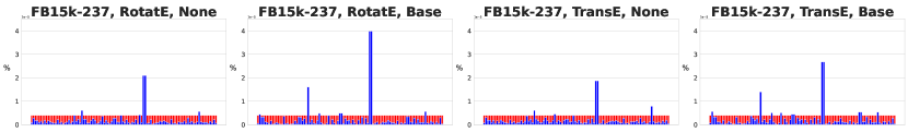
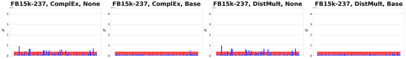
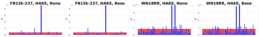
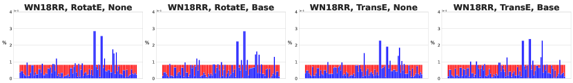
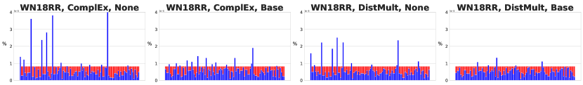
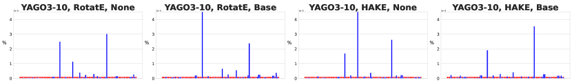
Figure 3: Appearance probabilities (%) of queries in CBS and MBS that have the lowest 100 CBS frequencies for each setting, sorted left to right in descending order by their CBS frequencies.

Metrics

We evaluated these methods using the most conventional metrics in KGC, i.e., Mean Reciprocal Rank (MRR), Hits@1 (H@1), Hits@3 (H@3), and Hits@10 (H@10). We reported the average scores in three different runs by changing their seeds for each metric. We also reported the standard deviations of the scores by the three runs.

Implementations and Hyper-parameters

For RotatE, TransE, ComplEx, and DistMult, we followed the implementations and hyper-parameters reported by Sun et al. (2019). For HAKE, we inherited the setting of Zhang et al. (2019).

In our experiments, the performance of subsampling is influenced by the selection of the following hyper-parameters: (1) temperature $\alpha$; (2) $\lambda$, the ratio of MBS against CBS. For our proposed MBS subsampling, we chose $\alpha$ from $\{2.0,1.0,0.5,0.1,0.05,0.01\}$ based on validation MRR. For our proposed MIX subsampling, we inherited the best $\alpha$ in MBS. Then, we chose the mix ratio $\lambda$ from $\{0.1,0.3,0.5,0.7,0.9\}$ based on validation MRR.

In FB15k-237 and WN18RR, we chose the sub-model from RotatE, TransE, HAKE, ComplEx, and DistMult with the setting of Base and None based on the validation MRR. In YAGO3-10, we also chose the sub-model from RotatE and HAKE, similar to FB15k-237 and WN18RR.

4.2 Results

Results

Table 3, 4, and 5 show the KGC performances on FB15k-237, WN18RR and YAGO3-10, respectively. Note that the results of Wilcoxon signed-rank test for performance differences between MBS/MIX and CBS show statistical significance with p-values less than 0.01 in all cases when MBS/MIX outperforms CBS.

As we can see, the models trained with MIX or MBS achieved the best results in all models on FB15k-237 and WN18RR. However, in YAGO3-10, HAKE with Freq in CBS outperformed the results of MBS and MIX. Considering that the preprocess of YAGO3-10 filtered out entities with less than 10 relations in the dataset, we can conclude that MBS and MIX are effective on the sparse KGs like that of FB15k-237 and WN18RR. These results are along with our expectation that MBS and MIX can improve the completion performances in sparse KGs as introduced in §1.

In individual comparison for each metric, CBS sometimes outperformed MIX or MBS. This is because the estimated frequencies in MIX and MBS rely on selected sub-models. From these results, we can understand that MIX and MBS have the potential to improve the KG completion performances by carefully choosing their sub-model.

Analysis

We analyze the remaining question, i.e., which sub-model to choose for MBS. Table 3, 4, and 5 show the selected sub-models for each MBS (See §4.1 in details), where ComplEx dominates over other models in FB15k-237 and WN18RR. To know the reason, we depict MBS frequencies of queries that have the bottom 100 CBS frequencies in Figure 3. In FB15k-237, we can see several spikes of frequencies in TransE, RotatE, and HAKE that do not exist in ComplEx. In WN18RR, the peak frequencies of ComplEx with None are larger and broader than that of other sub-models. These results indicate that models in FB15k-237 and WN18RR, respectively, encountered problems of an over and lack of smoothing, and MBS dealt with this problem. Because sparseness is a problem when data is small, these are along with the fact that FB15k-237 has larger training data than WN18RR. Thus, choosing a suitable sub-model for a target dataset is important in MBS.

Discussion

We discuss how sub-model and hyper-parameter choices contribute to the improvement of KGE performance apart from our method. The choice of the sub-model and the $\alpha$ played significant roles in the observed improvements because distributions from sub-model prediction depend on each sub-model and each dataset. Since we adopted the value of $\alpha$ used in the past state-of-the-art method of Sun et al. (2019) and Zhang et al. (2019), we believe that the performance gains of MBS are not only caused by the values of $\alpha$. Similarly, keeping $\lambda$ constant in the MIX strategy may lead to certain improvements depending on used sub-models and datasets. However, as shown in Appendix B, $\lambda$ has the role of adjusting the loss of multi-task learning, and thus, it may be more sensitive compared with $\alpha$.

5 Related Work

Mikolov et al. (2013) originally propose the NS loss to train their word embedding model, word2vec. Trouillon et al. (2016) introduce the NS loss to KGE to reduce training time. Sun et al. (2019) extend the NS loss for KGE by introducing a margin term, normalization of negative samples, and newly proposed their noise distribution. Kamigaito and Hayashi (2021) claim the importance of dealing with the sparseness problem of KGs through their theoretical analysis of the NS loss in KGE. Furthermore, Kamigaito and Hayashi (2022a) reveal that subsampling Mikolov et al. (2013) can alleviate the sparseness problem in the NS for KGE.

Similar to these works, our work aims to investigate and extend the NS loss used in KGE to improve KG performance.

6 Conclusion

In this paper, we propose new subsampling approaches, MBS and MIX, that can deal with the problem of low-frequent entity-relation pairs in CBS by estimating their frequencies using the sub-model prediction. Evaluation results on FB15k-237 and WN18RR showed the improvement of KGC performances by MBS and MIX. Furthermore, our analysis also revealed that selecting an appropriate sub-model for the target dataset is important for improving KGC performances.

Limitations

Utilizing our model-based subsampling requires pre-training for choosing a suitable sub-model, and thus may require more than twice the computational budget. However, since we can use a small model as a sub-model, like the use of ComplEx as a sub-model for HAKE, there is a possibility that the actual computational cost becomes less than the doubled one.

For calculating CBS frequencies, we only use the one with the arithmetic mean since we inherited the conventional subsampling methods as our baseline. Thus, we can consider various replacements not covered by this paper for the operation. However, even if we carefully choose the operation, CBS is essentially difficult to induce the appropriate appearance probabilities of low-frequent queries compared with our MBS, which can use vector-space embedding.

Our experiments are carried out only on FB15k-237, WN18RR, and YAGO3-10 datasets. Thus, whether our method works for larger and noisier data is to be verified.

Furthermore, although our method is generalizable to deep learning models, our current work is conducted purely on KGE models, and whether it works for general deep learning models as well is to be verified.

Appendix A Note on Figure 2

To illustrate the results on FB15k-237 and WN18RR datasets, we used TransE, RotatE, ComplEx, DistMult, and HAKE as the KGE models. To plot that on the YAGO3-10 dataset, we used RotatE and HAKE as the KGE models following the setting in §4.1. Regarding the use of subsampling, the MRR scores of using subsampling refer to the result of Base subsampling in Table 1 with CBS frequencies, whereas that without subsampling corresponds to the setting "None" §4.1.

Appendix B Interpretation of MIX Subsampling as Multi-task Learning

We can reformulate Eq. (16) as follows:

$$\ell_{mix}(\mathbf{\theta};\mathbf{\theta}^{\prime})$$ (19)

$$= -\frac{1}{|D|}\sum_{(x,y)\in D}\Bigl{[}A_{mix}(\mathbf{\theta}^{\prime})\log(\sigma(s_{\mathbf{\theta}}(x,y)+\gamma))+\frac{1}{\nu}\!\!\!\!\!\!\sum_{y_{i}\sim p_{n}(y_{i}|x)}^{\nu}\!\!\!\!\!\!B_{mix}(\mathbf{\theta}^{\prime})\log(\sigma(-s_{\mathbf{\theta}}(x,y_{i})-\gamma))\Bigr{]},$$ (20)

$$= -\frac{1}{|D|}\sum_{(x,y)\in D}\Bigl{[}(\lambda A_{mbs}(\mathbf{\theta}^{\prime})+(1-\lambda)A_{cbs})\log(\sigma(s_{\mathbf{\theta}}(x,y)+\gamma))$$

$$+\frac{1}{\nu}\!\!\!\!\!\!\sum_{y_{i}\sim p_{n}(y_{i}|x)}^{\nu}\!\!\!\!\!\!(\lambda B_{mbs}(\mathbf{\theta}^{\prime})+(1-\lambda)B_{cbs})\log(\sigma(-s_{\mathbf{\theta}}(x,y_{i})-\gamma))\Bigr{]},$$ (21)

$$= -\frac{\lambda}{|D|}\sum_{(x,y)\in D}\Bigl{[}A_{mbs}(\mathbf{\theta}^{\prime})\log(\sigma(s_{\mathbf{\theta}}(x,y)+\gamma))+\frac{1}{\nu}\!\!\!\!\!\!\sum_{y_{i}\sim p_{n}(y_{i}|x)}^{\nu}\!\!\!\!\!\!B_{mbs}(\mathbf{\theta}^{\prime})\log(\sigma(-s_{\mathbf{\theta}}(x,y_{i})-\gamma))\Bigr{]},$$

$$-\frac{1-\lambda}{|D|}\sum_{(x,y)\in D}\Bigl{[}A_{cbs}\log(\sigma(s_{\mathbf{\theta}}(x,y)+\gamma))+\frac{1}{\nu}\!\!\!\!\!\!\sum_{y_{i}\sim p_{n}(y_{i}|x)}^{\nu}\!\!\!\!\!\!B_{cbs}\log(\sigma(-s_{\mathbf{\theta}}(x,y_{i})-\gamma))\Bigr{]},$$ (22)

$$= \lambda\ell_{mbs}(\mathbf{\theta};\mathbf{\theta}^{\prime})+(1-\lambda)\ell_{cbs}(\mathbf{\theta})$$ (23)

From Eq. (23), since $\ell_{mix}(\mathbf{\theta};\mathbf{\theta}^{\prime})$ is the mixed loss of the two loss functions $\ell_{mbs}(\mathbf{\theta};\mathbf{\theta}^{\prime})$ and $\ell_{cbs}(\mathbf{\theta})$, we can understand that using MIX is multi-task learning of using both CBS and MBS.

References

- Bordes et al. (2013) Antoine Bordes, Nicolas Usunier, Alberto Garcia-Duran, Jason Weston, and Oksana Yakhnenko. 2013. Translating embeddings for modeling multi-relational data. In Advances in Neural Information Processing Systems, volume 26. Curran Associates, Inc.
- Dettmers et al. (2018) Tim Dettmers, Pasquale Minervini, Pontus Stenetorp, and Sebastian Riedel. 2018. Convolutional 2d knowledge graph embeddings. In AAAI.
- Guan et al. (2019) Jian Guan, Yansen Wang, and Minlie Huang. 2019. Story ending generation with incremental encoding and commonsense knowledge. Proceedings of the AAAI Conference on Artificial Intelligence, 33(01):6473–6480.
- Kamigaito and Hayashi (2021) Hidetaka Kamigaito and Katsuhiko Hayashi. 2021. Unified interpretation of softmax cross-entropy and negative sampling: With case study for knowledge graph embedding. In Proceedings of the 59th Annual Meeting of the Association for Computational Linguistics and the 11th International Joint Conference on Natural Language Processing (Volume 1: Long Papers), pages 5517–5531, Online. Association for Computational Linguistics.
- Kamigaito and Hayashi (2022a) Hidetaka Kamigaito and Katsuhiko Hayashi. 2022a. Comprehensive analysis of negative sampling in knowledge graph representation learning. In Proceedings of the 39th International Conference on Machine Learning, volume 162 of Proceedings of Machine Learning Research, pages 10661–10675. PMLR.
- Kamigaito and Hayashi (2022b) Hidetaka Kamigaito and Katsuhiko Hayashi. 2022b. Subsampling for knowledge graph embedding explained.
- Katz (1987) Slava Katz. 1987. Estimation of probabilities from sparse data for the language model component of a speech recognizer. IEEE transactions on acoustics, speech, and signal processing, 35(3):400–401.
- Lukovnikov et al. (2017) Denis Lukovnikov, Asja Fischer, Jens Lehmann, and Sören Auer. 2017. Neural network-based question answering over knowledge graphs on word and character level. In Proceedings of the 26th International Conference on World Wide Web, WWW ’17, page 1211–1220, Republic and Canton of Geneva, CHE. International World Wide Web Conferences Steering Committee.
- Mikolov et al. (2013) Tomás Mikolov, Ilya Sutskever, Kai Chen, Greg Corrado, and Jeffrey Dean. 2013. Distributed representations of words and phrases and their compositionality. CoRR, abs/1310.4546.
- Moon et al. (2019) Seungwhan Moon, Pararth Shah, Anuj Kumar, and Rajen Subba. 2019. OpenDialKG: Explainable conversational reasoning with attention-based walks over knowledge graphs. In Proceedings of the 57th Annual Meeting of the Association for Computational Linguistics, pages 845–854, Florence, Italy. Association for Computational Linguistics.
- Neubig and Dyer (2016) Graham Neubig and Chris Dyer. 2016. Generalizing and hybridizing count-based and neural language models. In Proceedings of the 2016 Conference on Empirical Methods in Natural Language Processing, pages 1163–1172, Austin, Texas. Association for Computational Linguistics.
- Sun et al. (2019) Zhiqing Sun, Zhi-Hong Deng, Jian-Yun Nie, and Jian Tang. 2019. Rotate: Knowledge graph embedding by relational rotation in complex space. In Proceedings of the 7th International Conference on Learning Representations, ICLR 2019.
- Toutanova and Chen (2015) Kristina Toutanova and Danqi Chen. 2015. Observed versus latent features for knowledge base and text inference. In Proceedings of the 3rd Workshop on Continuous Vector Space Models and their Compositionality, pages 57–66, Beijing, China. Association for Computational Linguistics.
- Trouillon et al. (2016) Théo Trouillon, Johannes Welbl, Sebastian Riedel, Éric Gaussier, and Guillaume Bouchard. 2016. Complex embeddings for simple link prediction. CoRR, abs/1606.06357.
- Yang et al. (2015) Bishan Yang, Wen tau Yih, Xiaodong He, Jianfeng Gao, and Li Deng. 2015. Embedding entities and relations for learning and inference in knowledge bases.
- Zhang et al. (2019) Zhanqiu Zhang, Jianyu Cai, Yongdong Zhang, and Jie Wang. 2019. Learning hierarchy-aware knowledge graph embeddings for link prediction.