Breakdown in vehicular traffic: driver over-acceleration, not over-reaction

Abstract

Contrary to a wide-accepted assumption about the decisive role of driver over-reaction for breakdown in vehicular traffic, we have shown that the cause of the breakdown is driver over-acceleration, not over-reaction. To reach this goal, we have introduced a mathematical approach for the description of driver over-acceleration in a microscopic traffic flow model. The model, in which no driver over-reaction occurs, explains all observed empirical nucleation features of traffic breakdown.

Traffic breakdown is a transition from free flow to congested vehicular traffic occurring mostly at bottlenecks. In 1958s-1961s, Herman, Gazis, Montroll, Potts, Rothery, and Chandler GM_Com as well as Kometani and Sasaki KS assumed that the cause of the breakdown is driver over-reaction on the deceleration of the preceding vehicle: Due to a delayed deceleration of the vehicle resulting from a driver reaction time the speed becomes less than the speed of the preceding vehicle. If this over-reaction is realized for all following drivers, then traffic instability occurs GM_Com ; KS ; Articles . The instability leads to a wide moving jam (J) formation in free flow (F) called as an F$\rightarrow$J transition KK1994 . The traffic instability is currently a theoretical basic of standard traffic theory (e.g., Articles ; Reviews ; Reviews2 ).

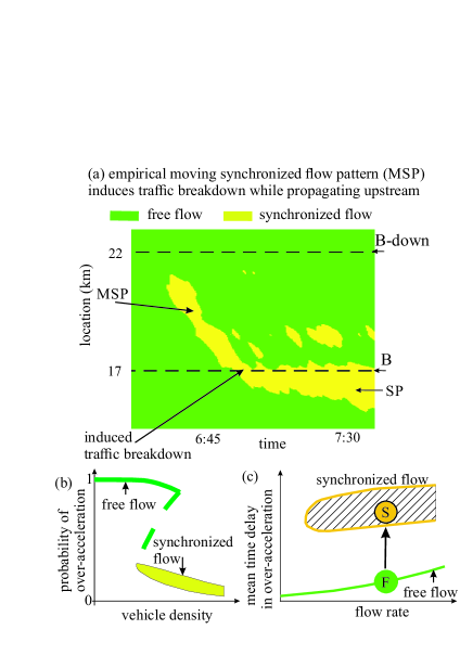
Figure 1: Empirical nucleation nature of traffic breakdown (F$\rightarrow$S transition) at bottlenecks (a) and hypothesis about discontinuous character of over-acceleration (b, c) OA . (a) Speed data presented in space and time with an averaging method were measured with road detectors installed along road: A moving synchronized flow pattern (MSP) that has emerged at downstream bottleneck (B-down) while propagating upstream induces F$\rightarrow$S transition (induced traffic breakdown) leading to emergence of synchronized flow pattern (SP) at upstream bottleneck (B); adapted from Three . (b, c) Qualitative density-dependence of over-acceleration probability per a time interval (b) and equivalent presentation of (b) as discontinuous flow-rate dependence of the mean time delay in over-acceleration (c); F and S are states of free flow and synchronized flow, respectively.

However, rather than the F$\rightarrow$J transition, in real field data traffic breakdown is a phase transition from free flow to synchronized flow (S) (F$\rightarrow$S transition) Three ; Three2 ; the empirical traffic breakdown exhibits the nucleation nature (Fig. 1(a)) . To explain the empirical nucleation nature of the F$\rightarrow$S transition, three-phase traffic theory was introduced Three , in which there are three phases: free flow (F), synchronized flow (S), and wide moving jam (J), where the phases S and J belong to congested traffic.

Driver over-reaction that should explain traffic breakdown can occur only if space gaps between vehicles are small enough GM_Com ; KS ; Articles ; KK1994 ; Reviews ; Reviews2 . At large enough gaps, rather than over-reaction, the vehicle speed does not become less than the speed of the decelerating preceding vehicle, i.e., usual speed adaptation to the speed of the preceding vehicle occurs that causes no instability.

• Contrary to standard theory GM_Com ; KS ; Articles ; KK1994 ; Reviews ; Reviews2 , it is assumed in three-phase traffic theory Three that traffic breakdown is realized at larger gaps between vehicles when no driver over-reaction can still occur.

In three-phase traffic theory, the empirical nucleation nature of the F$\rightarrow$S transition is explained through a hypothesis about a discontinuity in the probability of vehicle acceleration when free flow transforms into synchronized flow (Fig. 1(b)) OA : In free flow, vehicles can accelerate from car-following at a lower speed to a higher speed with a larger probability than it occurs in synchronized flow. Vehicle acceleration that probability exhibits the discontinuity when free flow transforms into synchronized flow is called over-acceleration, to distinguish over-acceleration from $``$usual” driver acceleration that does not show a discontinuous character. The discontinuous character of over-acceleration is explained as follows: Due to smaller space gaps in synchronized flow, vehicles prevent each other to accelerate from a local speed decrease; contrarily, due to larger space gaps in free flow at the same flow rate vehicles can easily accelerate from the local speed decrease. The discontinuous character of over-acceleration can lead to an S$\rightarrow$F instability in synchronized flow Three . Contrary to the classical traffic instability that is a growing wave of a local decrease in the vehicle speed GM_Com ; KS ; Articles ; KK1994 ; Reviews ; Reviews2 , the S$\rightarrow$F instability is a growing wave of a local increase in the speed Three . Microscopic three-phase models KKl that simulate the nucleation nature of traffic breakdown (Fig. 1(a)) show also the classical traffic instability leading to a wide moving jam emergence. In these complex traffic models KKl , both driver over-acceleration and driver over-reaction are important. Thus, up to now there has been no mathematical proof that the cause of the nucleation nature of traffic breakdown is solely over-acceleration without the influence of driver over-reaction.

Figure 2: Simulations with model (2)–(5) of nucleation nature of traffic breakdown (F$\rightarrow$S transition) on single-lane road of length $L=$ 10 km with two identical on-ramp bottlenecks B and B-down at road locations $x=x_{\rm on,B}=$ 6 km and $x=x_{\rm on,B-down}=$ 9 km, respectively: (a) Speed data presented in space and time as made in Fig. 1(a). (b, c) Averaged (1-min) speeds at $x=$ 7 km within MSP (b) and at $x=$ 5.7 km within SP induced through MSP propagation at bottleneck B. Flow rate on the road at $x=0$ is $q_{\rm in}=$ 2250 vehicles/h. For each of the bottlenecks that model is the same as that in AV_2023 , there is a merging region of length $L_{\rm m}=$ 0.3 km; vehicles merge at a middle location between vehicles on the road at the preceding vehicle speed $v^{+}$ when $g>g^{\rm(min)}_{\rm target}=\lambda_{\rm b}v^{+}+d$ with $\lambda_{\rm b}=$ 0.3 s; on-ramp inflow rates are $q_{\rm on,B-down}=$ 0 and $q_{\rm on,B}=$ 685 vehicles/h; to induce the MSP at bottleneck B-down, impulse $q_{\rm on,B-down}=$ 400 vehicles/h at $t=$ 20 min during 2 min has been applied. All vehicles in traffic flow are identical ones with the following model parameters: $\tau_{\rm safe}=$ 1 s, $\tau_{\rm G}=$ 3 s, $a_{\rm max}=$ 2.5 $\rm m/s^{2}$, $\alpha=$ 1 $\rm m/s^{2}$, $v_{\rm syn}=$ 80 km/h, $K_{\Delta v}=$ 0.8 $\rm s^{-1}$, $K_{1}=$ 0.15 $\rm s^{-2}$, $K_{2}=$ 0.95 $\rm s^{-1}$, $v_{\rm free}=$ 120 km/h, $d=$ 7.5 m. Under conditions $0\leq v\leq v_{\rm free}$, vehicle motion is found from equations $dv/dt=a$, $dx/dt=v$ solved with the second-order Runge-Kutta method with time step $10^{-2}$ s.

In the paper, we introduce a mathematical approach for over-acceleration $a_{\rm OA}$:

$$a_{\rm OA}=\alpha\Theta(v-v_{\rm syn})$$ (1)

that satisfies the hypothesis about the discontinuous character of over-acceleration (Fig. 1(b)). In (1), $v$ is the vehicle speed, where $0\leq v\leq v_{\rm free}$, $v_{\rm free}$ is a maximum speed; $\alpha$ is a maximum over-acceleration; $\Theta(z)=0$ at $z<0$ and $\Theta(z)=1$ at $z\geq 0$; $v_{\rm syn}$ is a given synchronized flow speed ($v_{\rm syn}<v_{\rm free}$).

Based on (1), we develop a microscopic traffic flow model, in which vehicle acceleration/deceleration $a$ in a road lane is described by a system of equations:

$$a = K_{\Delta v}\Delta v+a_{\rm OA}\ \textrm{at $g_{\rm safe}\leq g\leq G$},$$ (2)

$$a = a_{\rm max}\ \textrm{at $g>G$},$$ (3)

$$a = a_{\rm safety}(g,v,v_{\ell})\ \textrm{at $g<g_{\rm safe}$},$$ (4)

where $g$ is a space gap to the preceding vehicle, $\Delta v=v_{\ell}-v$, $v_{\ell}$ is the preceding vehicle speed, $K_{\Delta v}$ is a positive coefficient, $a_{\rm max}$ is a maximum acceleration, $G$ is a synchronization space-gap, $G=v\tau_{\rm G}$, $\tau_{\rm G}$ is a synchronization time headway, $g_{\rm safe}$ is a safe space-gap, $g_{\rm safe}=v\tau_{\rm safe}$, $\tau_{\rm safe}$ is a safe time headway, $a_{\rm safety}(g,v,v_{\ell})$ is a safety deceleration. The physics of model (2)–(4) is as follows:

(i) In Eq. (2), in addition to over-acceleration (1), there is function $K_{\Delta v}\Delta v$ Three ; KKl that describes vehicle speed adaptation to the preceding vehicle speed $v_{\ell}$ occurring independent of gap $g$ within the gap range $g_{\rm safe}\leq g\leq G$. Thus, a decrease in $v_{\ell}$ does not lead to a stronger decrease in the speed $v$: No driver over-reaction occurs.

(ii) Eq. (3) describes acceleration at large gaps $g>G$.

(iii) Contrary to over-acceleration $a_{\rm OA}$ (1) applied in Eq. (2), function $K_{\Delta v}\Delta v$ in Eq. (2) at $\Delta v>0$ and Eq. (3) describe $``$usual” acceleration that does not show a discontinuous character.

(iv) Eq. (4) describes safety deceleration that should prevent vehicle collisions at small gaps $g<g_{\rm safe}$; contrary to Eq. (2), safety deceleration $a_{\rm safety}(g,v,v_{\ell})$ in Eq. (4) can lead to driver over-reaction. There are many concepts developed in standard models GM_Com ; KS ; Articles ; KK1994 ; Reviews ; Reviews2 that can be used for safety deceleration $a_{\rm safety}(g,v,v_{\ell})$. For simulations below, we use one of them described by Helly’s function

$$a_{\rm safety}(g,v,v_{\ell})=K_{1}(g-g_{\rm safe})+K_{2}\Delta v,$$ (5)

where $K_{1}$ and $K_{2}$ dynamic coefficients .

Obviously, through an appropriated parameter choice in standard models GM_Com ; KS ; Articles ; KK1994 ; Reviews ; Reviews2 driver over-reaction is not realized even at the smallest possible gap $g=g_{\rm safe}$ in initial steady states of traffic flow. However, in this case no nucleation of congestion is possible to simulate with the standard models.

Contrarily, if we choose coefficients $K_{1}$ and $K_{2}$ in (5) (Fig. 2) at which even at $g\leq g_{\rm safe}$ no driver over-reaction occurs in model (2)–(5), then, nevertheless, this model shows all known empirical nucleation features of traffic breakdown (Fig. 1(a)): An MSP induced at downstream bottleneck B-down propagates upstream. While reaching upstream bottleneck B, the MSP induces F$\rightarrow$S transition at the bottleneck (Fig. 2).

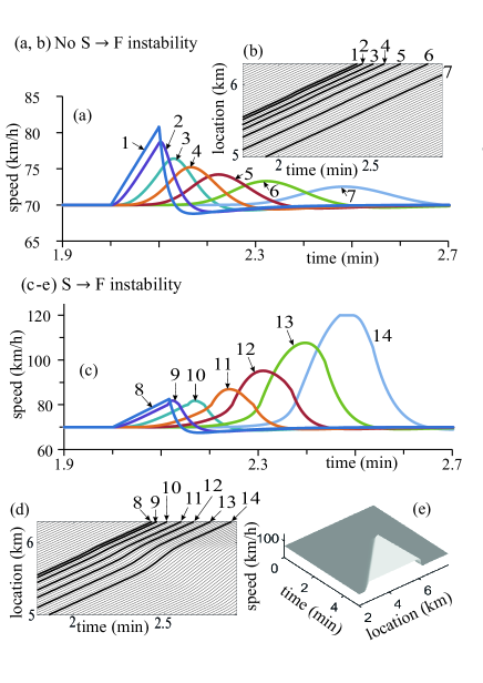
Figure 3: Nucleation character of S$\rightarrow$F instability simulated on single-lane road (8 km long) without bottlenecks with initial steady synchronized flow state at $v=$ 70 km/h and $g=$ 27.5 m: (a, b) No S$\rightarrow$F instability. (c–e) S$\rightarrow$F instability. In (a–d), time-development of speeds (a, c) and trajectories (b, d) of vehicles 1–7 (a, b) and 8–14 (c, d) caused by initial local speed increase of vehicle 1 (a, b) and vehicle 8 (c, d) simulated through vehicle short-time acceleration with $a=$ 0.5 $\rm m/s^{2}$ during 6.5 s in (a, b) and 7 s in (c, d). (e) Spatiotemporal development of speed during S$\rightarrow$F instability shown in (c, d). Other model parameters are the same as those in Fig. 2.

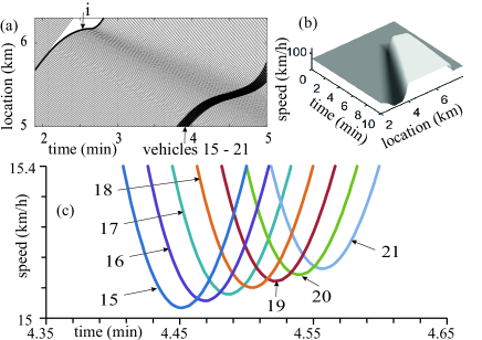
Figure 4: Absence of driver over-reaction in model (2)–(5) under parameters used in Fig. 2. Simulations made on single-lane road (8 km long) without bottlenecks with initial steady state of synchronized flow with $v=$ 70 km/h and $g=g_{\rm safe}=$ 19.5 m: Time-development of vehicle trajectories (a), speed in space and time (b), and speeds of a sequence of vehicles 15–21 caused by initial local speed decrease of vehicle $i$ in (a) simulated through deceleration of vehicle $i$ with $a=-$ 0.5 $\rm m/s^{2}$ to the speed $v=0$; vehicle $i$ remains stationary for 1 s and then accelerates.

Formula (1) for over-acceleration explains induced traffic breakdown as follows. Due to vehicle merging from on-ramp, condition $g<g_{\rm safe}$ can be satisfied resulting in vehicle deceleration: A local speed decrease occurs at bottleneck B (Fig. 2(a)). The minimum speed $v^{\rm(dec)}_{\rm min}$ within the local speed decrease satisfies condition $v^{\rm(dec)}_{\rm min}>v_{\rm syn}$. Therefore, according to (1), vehicles accelerate with over-acceleration $a_{\rm OA}=\alpha$ from the local speed decrease; this prevents congestion propagation upstream of bottleneck B. Contrarily, the minimum speed within the MSP satisfies condition $v^{\rm(MSP)}_{\rm min}<v_{\rm syn}$ (Fig. 2(b)). Then, according to (1), over-acceleration $a_{\rm OA}=0$: When the MSP reaches bottleneck B, synchronized flow is induced. The emergent SP remains at bottleneck B because the speed within the SP is less than $v_{\rm syn}$ in (1) (Fig. 2(c)) and, therefore, over-acceleration $a_{\rm OA}=0$. These simulations, in which no driver over-reaction can occur under chosen model parameters, support the statement of this paper:

• Traffic breakdown is caused by over-acceleration, not driver over-reaction.

Formula (1) for over-acceleration explains also the S$\rightarrow$F instability. We consider the time-development of a local speed increase in an initial steady synchronized flow state (Fig. 3). The cause of the local speed increase is a short-time acceleration of one of the vehicles (vehicle 1 in Figs. 3(a, b) or vehicle 8 in Figs. 3(c–e)); the vehicle must decelerate later to the speed of the preceding vehicle moving at the initial synchronized flow speed ($v=$ 70 km/h, Fig. 3). There are two possibilities: (i) The increase in the speed of following vehicles (vehicles 2–7 in Figs. 3(a, b)) decays over time (Figs. 3 (a, b)); this occurs when the maximum speed of vehicle 2 ($v^{\rm(2)}_{\rm max}=$ 77.9 km/h) is less than $v_{\rm syn}$ in (1) and, therefore, over-acceleration $a_{\rm OA}=0$. (ii) Contrarily, if vehicle 8 (Figs. 3(c, d)) accelerates only 0.5 s longer than vehicle 1 (Figs. 3(a, b)), the local speed increase initiated by vehicle 8 grows over time (vehicles 9–14 in Figs. 3(c, d)) leading to the S$\rightarrow$F instability (Figs. 3(c–e)); this occurs because the maximum speed of vehicle 9 ($v^{\rm(9)}_{\rm max}=$ 81.9 km/h) is higher than $v_{\rm syn}$ in (1) and, therefore, over-acceleration $a_{\rm OA}=\alpha$ causes the S$\rightarrow$F instability.

We have found that in model (2)–(5) under parameters used in Fig. 2 there is no driver over-reaction on the deceleration of the preceding vehicle even at the smallest possible space gap between vehicles $g=g_{\rm safe}$ in an initial homogeneous steady state of traffic flow. In Fig. 4, under condition $g=g_{\rm safe}$ in an initial synchronized flow, vehicle $i$ decelerates to a standstill, remains stationary for 1 s and then accelerates. It turns out that none of the following vehicles decelerates to the standstill. The minimum speed of the following vehicles increases slowly over time (vehicles 15–21 in Fig. 4(c)). Finally, rather than a wide moving jam (J), a new state of synchronized flow with speed $v\approx$ 15.5 km/h results from the deceleration of vehicle $i$.

Clearly, other model parameters in (2)–(5) in comparison with those used above (Figs. 2–4) can be chosen at which driver over-reaction occurs. In this case, simulations of the model show usual results of three-phase traffic theory Three ; KKl : (i) In free flow, the F$\rightarrow$S transition (traffic breakdown) occurs that features are qualitatively the same as presented in Figs. 2 and 3. (ii) Contrary to Fig. 4, in synchronized flow with lower speeds the classical traffic instability occurs leading to the S$\rightarrow$J transition. However, a detailed analysis of these results is out of the scope of the paper.

I thank Sergey Klenov for help in simulations and useful suggestions. I thank our partners for their support in the project $``$LUKAS – Lokales Umfeldmodell für das Kooperative, Automatisierte Fahren in komplexen Verkehrssituationen” funded by the German Federal Ministry for Economic Affairs and Climate Action.

References

- (1) R. E. Chandler, R. Herman, and E. W. Montroll, Oper. Res. 6, 165 (1958); R. Herman, E. W. Montroll, R. B. Potts, and R. W. Rothery, Oper. Res. 7, 86 (1959); D. C. Gazis, R. Herman, and R. B. Potts, Oper. Res. 7, 499 (1959); D. C. Gazis, R. Herman, and R. W. Rothery, Oper. Res. 9, 545 (1961).
- (2) E. Kometani and T. Sasaki, J. Oper. Res. Soc. Jap. 2, 11–26 (1958); Oper. Res. 7, 704–720 (1959); Oper. Res. Soc. Jap. 3, 176–190 (1961).
- (3) W. Helly, in Proceedings of the Symposium on Theory of Traffic Flow, Research Laboratories, General Motors (Elsevier, Amsterdam, 1959), pp. 207–238; G. F. Newell, Oper. Res. 9, 209 (1961); Transp. Res. B 36, 195 (2002); P. G. Gipps, Transp. Res. B 15, 105 (1981); Transp. Res. B. 20, 403 (1986); R. Wiedemann, Simulation des Verkehrsflusses (University of Karlsruhe, Karlsruhe, 1974); K. Nagel and M. Schreckenberg, J. Phys. (France) I 2, 2221 (1992); M. Bando, K. Hasebe, A. Nakayama, A. Shibata, and Y. Sugiyama, Phys. Rev. E 51, 1035 (1995); S. Krauß, P. Wagner, and C. Gawron, Phys. Rev. E 55, 5597 (1997); R. Barlović, L. Santen, A. Schadschneider, and M. Schreckenberg, Eur. Phys. J. B 5 793–800 (1998); T. Nagatani, Physica A 261, 599 (1998); Phys. Rev. E 59, 4857 (1999). M. Treiber, A. Hennecke, and D. Helbing, Phys. Rev. E 62, 1805 (2000).
- (4) B. S. Kerner and P. Konhäuser, Phys. Rev. E 48, R2335 (1993); 50, 54 (1994).
- (5) N. H. Gartner, C. J. Messer, A. Rathi (eds.), Traffic Flow Theory (Transportation Research Board, Washington, DC, 2001); J. Barceló (ed.), Fundamentals of Traffic Simulation, (Springer, Berlin, 2010); L. Elefteriadou, An introduction to traffic flow theory, in Springer Optimization and its Applications, Vol. 84 (Springer, Berlin, 2014); Daiheng Ni, Traffic Flow Theory, (Elsevier, Amsterdam, 2015).
- (6) D. Chowdhury, L. Santen, and A. Schadschneider, Phys. Rep. 329, 199 (2000); D. Helbing, Rev. Mod. Phys. 73, 1067 (2001); T. Nagatani, Rep. Prog. Phys. 65, 1331 (2002); K. Nagel, P. Wagner, and R. Woesler, Oper. Res. 51, 681 (2003); M. Treiber and A. Kesting, Traffic Flow Dynamics (Springer, Berlin, 2013); A. Schadschneider, D. Chowdhury, K. Nishinari, Stochastic Transport in Complex Systems, (Elsevier Science Inc., New York, 2011).
- (7) B. S. Kerner, The Physics of Traffic (Springer, Berlin, New York, 2004); Introduction to Modern Traffic Flow Theory and Control (Springer, Berlin, 2009); Breakdown in Traffic Networks (Springer, Berlin/New York, 2017); Understanding Real Traffic (Springer, Cham, 2021).
- (8) H. Rehborn, M. Koller, and S. Kaufmann, Data-Driven Traffic Engineering, (Elsevier, Amsterdam, 2021).
- (9) M.J. Lighthill and G.B. Whitham, Proc. Roy. Soc. A 229, 281 (1955); P.I. Richards, Oper. Res. 4, 42–51 (1956); A.D. May, Traffic Flow Fundamentals (Prentice-Hall, Hoboken, NJ, 1990); C.F. Daganzo, Transp. Res. B 28, 269 (1994); Transp. Res. B 29, 79 (1995); Highway Capacity Manual, 6th ed., National Research Council (Transportation Research Board, Washington, DC, 2016).
- (10) B. S. Kerner, Phys. World 12, 25 (1999); Trans. Res. Rec. 1678, 160 (1999); J. Phys. A: Math. Gen. 33, L221 (2000); Phys. Rev. E 65, 046138 (2002).
- (11) B.S. Kerner, S.L. Klenov, J. Phys. A: Math. Gen. 35, L31–L43 (2002); Phys. Rev. E 68 036130 (2003); J. Phys. A: Math. Gen. 39, 1775 (2006); B.S. Kerner, S.L. Klenov, and D.E. Wolf, J. Phys. A: Math. Gen. 35, 9971 (2002).
- (12) B. S. Kerner, Phys. Rev. E 100, 012303 (2019).
- (13) H.K. Lee, R. Barlović, M. Schreckenberg, D. Kim, Phys. Rev. Lett. 92 238702 (2004).
- (14) B. S. Kerner, Phys. Rev. E 108, 014302 (2023).