A non-perturbative formula unifying double-wells and anharmonic oscillators under the numerical bootstrap approach

Abstract

We study the energy gap between the ground state and the first excited state of quantum anharmonic oscillators, using the numerical bootstrap method. Based on perturbative formulae of limiting coupling regimes, we propose a qualitative formula of the energy gap across all coupling values, connecting the limiting regimes. Except detailed numerical parameter values, the proposed formula has the same functional form as the formula of ground state level splitting of double-well potentials, proposed recently in arXiv:2308.11516. This connects the anharmonic oscillators with the double-well potentials, although the underlying physics of them are different. The proposed formula is justified on bootstrap data up to the octic anharmonicities.

I Introduction

In a recent paper [1], we studied the ground state level splitting $\Delta E_{D}$ caused by instantons in double-well potential models. We proposed a qualitative formula for $\Delta E_{D}$ across all coupling values, so it describes both the ’weak’ and the ’strong’ regime of instanton effects. For the quartic case, it agrees with the known perturbative behaviors at limiting coupling regimes. The proposed formula is justified on numerical data for the quartic and the sextic double-well potential, obtained from the numerical bootstrap. Results suggest that the proposed formula works for symmetric double-well of all anharmonicities, only with different numerical parameter values for different anharmonicities.

In the present paper, we study the energy gap $\Delta E$ between the ground state and the first excited state of quantum anharmonic oscillators. This work is very natural, since the double-well potentials become anharmonic oscillators after changing the sign of coupling constant $g$ from minus to plus. Quantum anharmonic oscillators play an important role in perturbation theory [2, 3]. In the weak regime of anharmonicity, the bare states are harmonic oscillators and the energy levels are asymptotic series, which is the famous large-order perturbation expansion firstly obtained by WKB methods [4, 5]. This asymptotic series is Borel summable [6] and is connected with the decay rate of inverted double-well potentials [7, 8, 9, 10]. On the complex plane, the dispersion relation connects the large-order behavior of energy on the right hand (positive coupling, thus anharmonic oscillators) with the discontinuity of energy on the left hand (negative coupling, thus the inverted double-well potential) [2, 3].

It is an interesting question to ask what is the analytic structure of the strong anharmonicity regime. In the strong regime, the bare states are unknown and the energy levels are computed by numerical convergent series. Here we propose a qualitative formula across all coupling values, connecting the two limiting regimes. The proposed formula here has the same functional form as the one proposed in our recent paper [1] for the ground state level splitting of double-well potentials, and this suggests that there might be a connection between anharmonic oscillators and double-well potentials. This is different from the perturbation in the weak regime, where anharmonic oscillators are connected to the inverted double-well potentials via the dispersion relation.

We test our proposed formula on numerical data up to the octic anharmonic oscillator. The data is computed by the non-perturbative numerical bootstrap method, where the spectrum is solved from a set of consistency conditions that are built using only elementary properties of quantum theory without any perturbations. It relies on the semidefinite programming algorithm [11, 12, 13, 14] and has rapidly developing applications in various fields of physics [15, 16, 17, 18, 19, 20, 21, 22, 23, 24, 25, 26, 27, 28, 29, 30, 31, 32, 33, 34, 35, 36, 37, 38, 39, 40, 41, 42, 43, 44, 45, 46, 47, 48]. For applying the numerical bootstrap to anharmonic oscillators, the algorithm has been studied in great detail by  [22, 23, 24, 25, 26, 27, 28, 29, 30]. As in [1], here we follow the implementation introduced firstly by [23].

In the following, we will firstly review steps of the numerical bootstrap method. Then we define the models and analyze their bootstrap data. We propose the qualitative formula (12) after introducing the one-loop formula (9) of the quartic anharmonic oscillator, making it convenient to discuss the detailed physics there. In the end we close with a discussion of open questions and future work.

II Method of the numerical bootstrap

For the reason of completeness, here we repeat the brief review of numerical bootstrap already given in our previous paper [1]. The readers familiar with it may skip this part. For the practical implementation, we follow the choice of operators $\{x^{m}p^{n}\}$ introduced firstly by [23]. The algorithmic details have been analyzed extensively from various aspects, and the interested reader can go to references listed in the Introduction.

The numerical bootstrap divides into three steps: (1) choose a set of operators and derive their recursive equations, (2) impose positive constraints (or other working constraints) on the operators and obtain the bootstrap matrix, (3) set the numerical search space and use the semidefinite optimization to find allowed parameter values in this space. Here for anharmonic oscillators, we choose the system energy as the search parameter, because our aim is to compute the energy of the ground state and the first excited state.

II.1 Recursive equations

For a quantum mechanical system, we use the following Hamiltonian:

$$H=\frac{p^{2}}{2}+V(x)$$ (1)

For its energy eigenstate $\left|\varphi\right\rangle$ with eigenvalue $E$, the expectation value of operators composed of $H$ and an arbitrary operator $\alpha$, must satisfy the following two constrains,

$$\left\langle{\left[{H,\alpha}\right]}\right\rangle\equiv\left\langle\varphi|{\left[{H,\alpha}\right]}|\varphi\right\rangle=0,\,\left\langle{H\alpha}\right\rangle=\left\langle{\alpha H}\right\rangle=E\left\langle\alpha\right\rangle$$ (2)

If choose $\alpha={x^{n}},{x^{n}}p$, these constrains lead to the following recursion relations [23, 26]

$$n(n-1)(n-2) \left\langle{{x^{n-3}}}\right\rangle-8n\left\langle{{x^{n-1}}V(x)}\right\rangle$$ (3)

$$+8nE\left\langle{{x^{n-1}}}\right\rangle-4\left\langle{{x^{n}}{V^{\prime}}(x)}\right\rangle=0.$$

II.2 bootstrap matrix

To build the bootstrap matrix, we follow the efficient construction proposed by [23] by choosing the following operators,

$$\mathcal{O}=\sum\limits_{m=0}^{k_{x}}\sum\limits_{n=0}^{k_{p}}{{C_{mn}}{x^{m}}{p^{n}}}$$ (4)

with ${C_{mn}}$ being constants. The expectation value of the operator $\mathcal{O}$ on the energy eigenstate $\left|\varphi\right\rangle$ satisfies the positivity constraint

$$\left\langle{{{\mathcal{O}}^{\dagger}}{\mathcal{O}}}\right\rangle\geq 0.$$ (5)

From this constraint, the bootstrap matrix can be built that must be positive-semidefinite

$${M}:=\left({\begin{array}[]{*{20}{c}}{{\mathcal{O}}_{0}^{{\dagger}}{{\mathcal{O}}_{0}}}&{{\mathcal{O}}_{0}^{{\dagger}}{{\mathcal{O}}_{1}}}&\ldots&{{\mathcal{O}}_{0}^{{\dagger}}{{\mathcal{O}}_{k}}}\\ {{\mathcal{O}}_{1}^{{\dagger}}{{\mathcal{O}}_{0}}}&{{\mathcal{O}}_{1}^{{\dagger}}{{\mathcal{O}}_{1}}}&\ldots&{{\mathcal{O}}_{1}^{{\dagger}}{{\mathcal{O}}_{k}}}\\ \vdots&\vdots&\ddots&\vdots\\ {{\mathcal{O}}_{k}^{{\dagger}}{{\mathcal{O}}_{0}}}&{{\mathcal{O}}_{k}^{{\dagger}}{{\mathcal{O}}_{1}}}&\ldots&{{\mathcal{O}}_{k}^{{\dagger}}{{\mathcal{O}}_{k}}}\end{array}}\right)\geq 0,$$ (6)

where $\mathcal{O}_{0,1,2,\ldots}$ are the component operators of $\mathcal{O}$ and the maximum value $k$ is called the depth of the bootstrap matrix. As the depth $k$ increases, the positive-semidefinite constraint becomes stronger and so the numerical results becomes more accurate.

II.3 Search space

The last step is to set the search space which is a minimum set of data to initialize the recursion. After choosing search parameters and the optimization target, the positive-semidefinite optimization will exclude parameter values that do not satisfy the constraints (6) and so reduce the size of the parameter space. With sufficiently large depth $k$, the remaining parameter space passing the constraints (6) will be a tiny neighborhood that can be viewed as a data point. This data point is the discrete eigenvalue of the quantum system with the optimized target value being the expectation. The search space of the quartic anharmonic oscillator is $\left\{E,{\rm{}}\left\langle{{x^{2}}}\right\rangle\right\}$, the sextic case is $\left\{{E,{\rm{}}\left\langle{{x^{2}}}\right\rangle,{\rm{}}\left\langle{{x^{4}}}\right\rangle}\right\}$ and the octic case is $\left\{{E,{\rm{}}\left\langle{{x^{2}}}\right\rangle,{\rm{}}\left\langle{{x^{4}}}\right\rangle,\left\langle{{x^{6}}}\right\rangle}\right\}$.

An example of the bootstrap data is shown in Figure 1 for the octic oscillator at $g=1$. For small depth $k=7$, the ground state is separated from excited states, but the resolution is very low. As the depth increases to $k=13$, the ground state and the first excited states are identified to a high resolution, and higher excited states are separated out. At this depth $k=13$ the bootstrap matrix is not large, so this implementation [23] is very efficient. This behavior with depth $k$ is the same as that in [1] for double-well potentials.

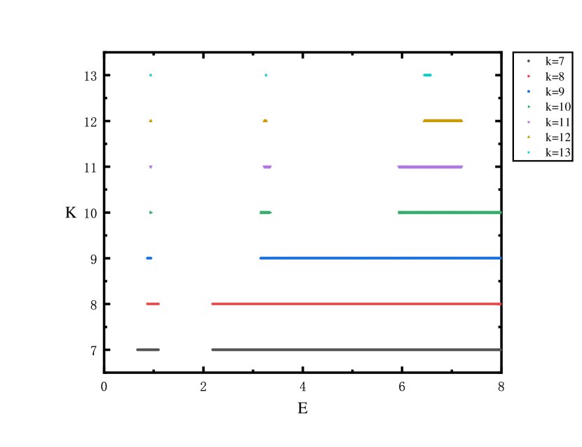
Figure 1: An example bootstrap data of the octic oscillator at $g=1$ for various depth $k$ of bootstrap matrix.

III Bootstraping anharmonic oscillators

The pure anharmonic oscillator is defined as

$$H=\frac{p^{2}}{2}+gx^{2}+x^{2n},\quad g>0\,\&\,n\geq 2.$$ (7)

When $g<0$, this becomes the double-well potential studied in [1]. In this convention, the coupling $g$ is of the ’mass’ term : large coupling $g\gg 1$ is the weak regime of anharmonicity and small coupling $g\to 0$ is the strong regime of anharmonicity. We will compute its energy gap between the ground state $E_{0}$ and the first excited state $E_{1}$ using the numerical bootstrap

$$\Delta E=E_{1}-E_{0}=\Delta E^{\prime}+\sqrt{2g},$$ (8)

where in the last step $\sqrt{2g}$ is the energy gap of harmonic oscillators. It is a standard practice to separate out the energy levels of harmonic oscillators, when studying the energy levels of anharmonic oscillators [3, 2].

In the weak regime of the quartic anharmonic oscillator, the asymptotic series of $E_{0}$ can be recast as a closed formula by the one-loop path integral [3]

$$E_{0}(g)=\sqrt{\frac{g}{2}}+\frac{\sqrt{6}g-\sqrt{2\pi}e^{\frac{g^{3}}{3}}g^{5/2}\operatorname{erfc}\left(\frac{g^{3/2}}{\sqrt{3}}\right)}{\pi},$$ (9)

where $\operatorname{erfc}(z)$ is the complementary error function. In the harmonic limit $g\to\infty$, the asymptotic expansion of $\operatorname{erfc}(z)$  [49]

$$\operatorname{erfc}(z)\displaystyle\sim\frac{e^{-z^{2}}}{\sqrt{\pi}}\sum_{m=0}^{\infty}(-1)^{m}\frac{{\left(\tfrac{1}{2}\right)_{m}}}{z^{2m+1}}$$ (10)

gives the correct ground state energy of harmonic oscillators

$$E_{0}(g)\displaystyle\sim\sqrt{\frac{g}{2}}+\frac{3\sqrt{\frac{3}{2}}}{\pi g^{2}}+O\left(\frac{1}{g^{9/2}}\right)\sim\sqrt{\frac{g}{2}}.$$ (11)

Higher energy levels can be computed as a series with numerical coefficients using the variational approach to tunneling [50], but there is no closed formula like (9). In the strong regime of anharmonicity, $g\to 0$ of  (9) gives $E_{0}=0$ which is obviously wrong. So the one-loop perturbation (9) can not describe the strong regime. In the strong regime, energy levels are usually given as numerical convergent series.

From an educated guess, we propose the following formula of the energy gap $\Delta E^{\prime}$ due to the anharmonicity

$$\Delta E^{\prime}(g)=2\Delta E^{\prime}(0)\frac{e^{-ag^{b}}}{1+e^{-cg^{d}}},\quad a,b,c,d>0,$$ (12)

with numerical parameter values depending on the anharmonicity order $n$. In the harmonic limit $g\to\infty$ this is zero, so it correctly reduces to the hamonic oscillator. In the strong regime $g\to 0$, this is a convergent series of $g$ as expected. This happens to be the formula proposed in [1] for the ground state level splitting of double-well potentials. This suggests there is a connection between them, which will be discussed later.

III.1 Quartic oscillator

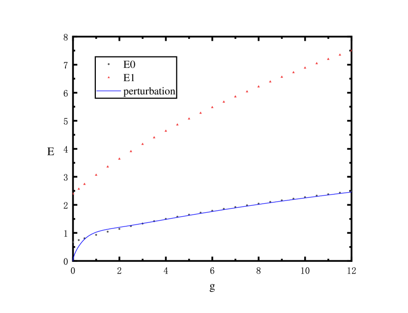
(a) Energy levels $E_{0}$ and $E_{1}$.

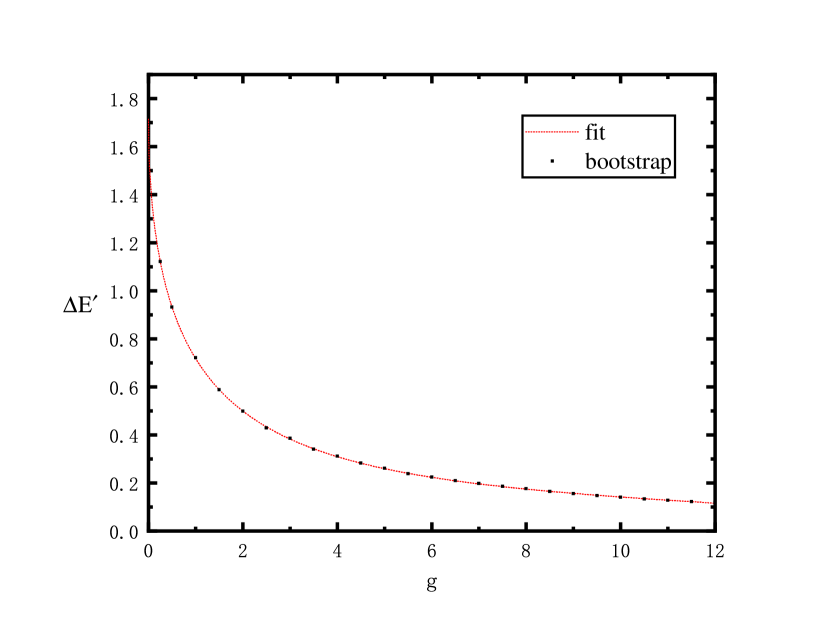
(b) $\Delta E^{\prime}$

Figure 2: The quartic oscillator.

For the quartic oscillator, Figure 2(a) shows the bootstrap data of $E_{0}$ and $E_{1}$, and the perturbation formula (9) of $E_{0}$. In the weak anharmonicity regime $g\gg 1$, the perturbation approaches the bootstrap data and captures the main physics of the ground state. In the strong regime $g\to 0$, the perturbation formula of asymptotic series (9) fails completely. This strong regime can be described by convergent numerical series [3, 2] of $g$, but the convergent series fails in the weak regime. This is expected of perturbation theory that it is valid only near the regime where it is expanded.

Figure 2(b) shows the energy gap $\Delta E^{\prime}$ due to the anharmonicity and the proposed formula $\Delta E^{\prime}(g)$ (12) fitted to the data. The data $\Delta E^{\prime}$ is maximum at $g=0$ and then quickly drops. When $g\gg 1$, it goes to zero asymptotically, which is the reason of the tiny deviation between the data $E_{0}$ and the formula (9) in Figure 2(a). This asymptotic decreasing behavior of $\Delta E^{\prime}$ is expected and it explains why perturbative energy levels in the weak regime are asymptotic series like (9). The proposed formula $\Delta E^{\prime}(g)$ (12) fits well with the data, with parameter values given in Table 1. Here we emphasize that, the sole purpose of data fitting is to justify the qualitative formula (12). The true parameters $a,b,c,d$ should be determined analytically, maybe from a renormalization-group-like procedure as argued in [1], and the numerically fitted values should not be taken as something exact or something serious.

III.2 Sextic oscillator

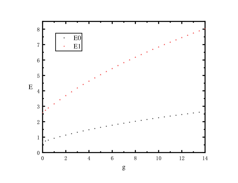
(a) Energy levels $E_{0}$ and $E_{1}$.

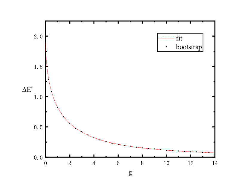
(b) $\Delta E^{\prime}$

Figure 3: The sextic oscillator.

For the sextic oscillator, Figure 3(a) shows the bootstrap data of $E_{0}$ and $E_{1}$, and Figure 3(b) shows the energy gap $\Delta E^{\prime}$ due to the anharmonicity. We see similar behavior of $\Delta E^{\prime}$ as in the quartic case. The proposed formula $\Delta E^{\prime}(g)$ (12) fits well with the data, with parameter values given in Table 1.

III.3 Octic oscillator

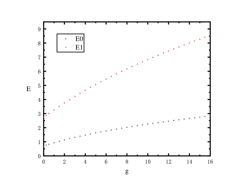
(a) Energy levels $E_{0}$ and $E_{1}$.

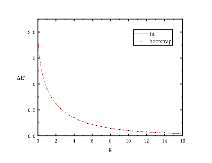
(b) $\Delta E^{\prime}$

Figure 4: The octic oscillator.

For the octic oscillator, Figure 4(a) shows the bootstrap data of $E_{0}$ and $E_{1}$, and Figure 4(b) shows the energy gap $\Delta E^{\prime}$ due to the anharmonicity. Again behavior of $\Delta E^{\prime}$ is the same as the other cases. The proposed formula $\Delta E^{\prime}(g)$ (12) fits well with the data, with parameter values given in Table 1.

	n=2	n=3	n=4
a	0.8842629827697163	0.8421595166826806	0.8014327779076852
b	0.5193664589411509	0.5597339573586666	0.5720036705632807
c	0.015270747582868331	0.008140628665542498	0.0015383208190051754
d	1.888568625833652	1.8560295155792268	1.3556010103295226

Table 1: Fitted parameter values of (12) for anharmonic oscillators $gx^{2}+x^{2n}$.

III.4 Unifying with double-well potentials

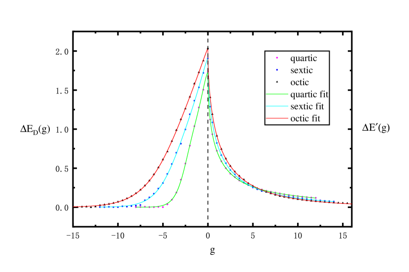
Figure 5: $\Delta E^{\prime}(g)$ and $\Delta E_{D}(g)$ for the quantum system $V(x)=gx^{2}+x^{2n}$

The proposed formula $\Delta E^{\prime}(g>0)$ (12) here for anharmonic oscillators is the same formula $\Delta E_{D}(g<0)$ proposed in [1] for double-well potentials. To understand this unexpected connection, let’s treat anharmonic oscillators and double-well potentials as a single quantum system $V(x)=gx^{2}+x^{2n}$, then $g>0$ and $g<0$ can be viewed as two ’phases’ with oscillator physics and instanton physics respectively. Like in quantum phase transitions, the energy gap $\Delta E=E_{1}-E_{0}$ between the ground state and the first excited state is the order parameter [51] and characterizes the behavior of the system. For $\Delta E$ of anharmonic oscillators $g>0$, we subtract from it the energy gap $\sqrt{2g}$ of harmonic oscillators and focus on $\Delta E^{\prime}(g)=\Delta E-\sqrt{2g}$. Since the limiting weak regime is the harmonic oscillator, $\Delta E^{\prime}(g)$ captures the deviation from this limiting regime due to anharmonicity. For double-well potentials $g<0$, the energy gap $\Delta E$ at finite $g$ is also called the ground state level splitting due to instantons. Since the limiting weak regime is the degenerated harmonic oscillators of zero level splitting, we can view the quantity $\Delta E_{D}(g)=\Delta E(g)-0$ as capturing the deviation from this limiting regime, like $\Delta E^{\prime}(g)$ of anharmonic oscillators.

With this view of $\Delta E^{\prime}(g)$ and $\Delta E_{D}(g)$, Figure 5 shows them together with data up to the octic case. The data of double-well potentials is taken from [1]. In the ’phase’ $g<0$, it shows the data of $\Delta E_{D}(g)$ coming from instanton physics. In the ’phase’ $g>0$, it shows the data of $\Delta E^{\prime}(g)$ coming form oscillator physics. In both ’phases’, the proposed formula (12) agrees well with the data, which suggests a deep connection between anharmonic oscillators and double-well potentials. Furthermore, they all look like a $\lambda\operatorname{-shape}$ curve that is common in phase transitions [52]. So this suggests a stronger analog with phase transitions.

IV Conclusion

In this work, we studied the energy gap $\Delta E^{\prime}(g)=E_{1}-E_{0}-\sqrt{2g}$ of quantum anharmonic oscillators, where the energy gap $\sqrt{2g}$ of pure harmonic oscillators is subtracted off. So $\Delta E^{\prime}(g)$ captures the deviation from the limiting harmonic regime due to anharmonicity. We used the numerical bootstrap method following [23] for the detailed implementation of the algorithm. We proposed a qualitative formula (12) for $\Delta E^{\prime}(g)$ across all coupling values, with the expected behavior both in the strong and the weak regime. It is tested on bootstrap data up to the octic anharmonic oscillator and works well. Here we choose the numerical bootstrap method because of its non-perturbative nature: the only artificial factor is to increase the depth of the bootstrap matrix.

The proposed formula here for $\Delta E^{\prime}(g)$ (12) happens to be the same formula that we [1] propose for the ground state level splitting $\Delta E_{D}(g)$ of double-well potentials. In fact, this study is a natural follow up of our recent study [1] of double-well potentials, because they can be viewed as the same model $V(x)=gx^{2}+x^{2n}$ with $g>0$ (oscillators) and $g<0$ (double-wells) respectively. When viewing $g>0$ as the ’phase’ of oscillators and $g<0$ as the ’phase’ of instantons, Figure 5, the plot of $\Delta E^{\prime}(g)$ and $\Delta E_{D}(g)$, resembles $\lambda\operatorname{-shape}$ curves common of phase transitions. This might only be a coincidence. Or this might suggest a new connection between anharmonic oscillators and double-well potentials, from the view point of quantum phase transitions.

The oscillator physics dominates $\Delta E^{\prime}(g)$ and the instanton physics dominates $\Delta E_{D}(g)$, so it is unexpected that they share the same formula (12). This suggests a deep connection between anharmonic oscillators and double-well potentials. In perturbation theory of anharmonic oscillators near the weak anharmonicity regime, the dispersion relation connects the large-order asymptotic expansion of energy with the discontinuity of energy of inverted double-well potentials. Our proposed formula suggests there might be an analytic connection between anharmonic oscillators and double-well potentials. This suggestion is not alone. In [53], the perturbation series of anharmonic oscillators and double-well potentials are connected by introducing an effective mass and reexpansion of series.

We hope that our finding can serve as a guide for searching an analytic method that works both at the ’weak’ and the ’strong’ regime. There are works on this direction. For example, in [54, 55] energy levels in the weak and the strong regime are linked by a Laplace integral representation. The connection between anharmonic oscillators and double-well potentials we find here might help this search.