Distinguishable consequence of classical gravity on quantum matter

Abstract

What if gravity is classical? If true, a consistent co-existence of classical gravity and quantum matter requires that gravity exhibit irreducible classical fluctuations. These fluctuations can mediate classical correlations between the quantized motion of the gravitationally interacting matter. We use a consistent theory of quantum-classical dynamics, together with general relativity, to show that experimentally relevant observables can conclusively test the hypothesis that gravity is classical. This can be done for example by letting highly coherent source masses interact with each other gravitationally, and performing precise measurements of the cross-correlation of their motion. Theory predicts a characteristic phase response that distinguishes classical gravity from quantum gravity, and from naive sources of decoherence. Such experiments are imminently viable.

Introduction. It is believed that if gravitational source masses can be prepared in quantum superpositions, then the gravitational field sourced by them has to be quantum. Feynman’s argument in support [1] relies on the expectation that a double-slit experiment with two massive particles produces an interference pattern. If the gravitational fields sourced by them are assumed to be classical, then it can convey the which-path information that contradicts the development of the interference pattern. So for consistency, the gravitational field needs to be quantum, so that its quantum fluctuations obfuscate the which-path information (see also [2, 3]). An equally viable hypothesis that achieves consistency is that the gravitational field is classical and stochastic [4, 5, 6, 7, 8], so that it cannot convey precise which-path information.

Contrary to the hypothesis that gravity is quantum [9, 10], a stochastic classical gravity will not entangle the source masses. But since the field is a dynamical entity, it can mediate classical correlations between the motion of the source masses. It is precisely this subtle detail that is missing by naively adopting the view that the only effect of classical stochastic gravity is the decoherence of the source masses [11, 12, 13, 14, 15, 16, 17, 18]. It certainly does, but it leaves a telltale sign distinct from quantum gravity, and from other extraneous sources of decoherence.

We describe a consistent and generic low-energy theory of classical gravity interacting with quantum source masses, and produce experimentally relevant signatures of such a theory. These signatures are smoking-gun evidence for the hypothesis that gravity is classical. Crucially, these predictions are sensitive to the difference between a classical description of gravity and an effective quantum theory of gravitation [19, 20, 21, 22, 23, 24, 25], and can be tested without macroscopic masses in quantum superpositions [26, 27].

Classical-quantum theory. Even if gravity is classical, it is necessary that when a quantized mass interacts with it, the ensuing dynamics does not prevent the assignment of a legitimate joint state. That is, there exists a positive-definite unit-trace operator $\hat{\rho}_{t}(z)$ in the Hilbert space of the quantum object for each classical state $z$ in the phase space of the classical gravitational field. The (quantum) state of the mass alone is $\hat{\rho}_{Q}=\int\differential{z}\hat{\rho}_{t}(z)$, while the (classical) state of the field alone is $p_{t}(z)=\Tr\hat{\rho}_{t}(z)$. The general structure of the dynamics of $\hat{\rho}_{t}(z)$ is [28, 29, 30, 31, 6, 7]

$$\begin{split}\dot{\hat{\rho}}_{t}=&-i[\hat{H}_{t},\hat{\rho}_{t}]+Q_{\alpha\beta}\left(\hat{L}_{\alpha}\hat{\rho}_{t}\hat{L}_{\beta}^{\dagger}-\frac{1}{2}[\hat{L}_{\beta}^{\dagger}\hat{L}_{\alpha},\hat{\rho}_{t}]_{+}\right)\\ &+\partial_{z_{i}}\left(C_{i}\hat{\rho}_{t}\right)+\partial_{z_{i}z_{j}}\left(C_{ij}\hat{\rho}_{t}\right)\\ &+\partial_{z_{i}}\left(M_{\alpha i}\hat{\rho}_{t}\hat{L}^{\dagger}_{\alpha}+\mathrm{{h.c.}}\right).\end{split}$$ (1)

This equation consists of several qualitatively distinct terms: the first row describes pure quantum state evolution by the Hamiltonian $\hat{H}_{t}(z)$ and quantum diffusion described by the Lindblad operators $\{\hat{L}_{\alpha}\}$ with diffusion constants $Q_{\alpha\beta}(z)$; the second row, as we shall see, describes classical pure state evolution and diffusion with constants $C_{i}(z)$ and $C_{ij}(z)$; and the last line is “classical-quantum diffusion” with constants $M_{\alpha i}(z)$.

Note that the classical-quantum model of Eq. 1 resolves the pathologies of a semi-classical description of gravity [32]. Since the model describes the co-evolution of quantum matter and classical gravity via their mutual back-action, prior experiments where quantum systems evolve in a static gravitational potential [33, 34, 35, 36, 37, 38, 39] have not tested this model.

The state of the classical system $p_{t}(z)$ obeys classical Hamiltonian dynamics under the Hamiltonian $H_{C}$ if $\partial_{z_{i}}C_{i}=0$ and $C_{j}+J_{ij}\partial_{z_{i}}H_{C}=0$; here $J$ is the symplectic matrix. Under these conditions, $\Tr[\partial_{z_{i}}(C_{i}\hat{\rho})]=J_{ij}(\partial_{z_{i}}H_{C})(\partial_{z_{j}}p)=\{H_{C},p\}$, where $\{\cdot,\cdot\}$ is the Poisson bracket. If a similar set of conditions are imposed on the coefficients $M_{\alpha i}$, namely that, $\partial_{z_{i}}M_{\alpha i}=0$ and $M_{\alpha j}+J_{ij}(\partial_{z_{i}}h_{\alpha})=0$, for some function $h_{\alpha}$, then $\Tr[\partial_{z_{i}}(M_{\alpha i}\hat{\rho}\hat{L}_{\alpha}^{\dagger}+\mathrm{{h.c.}})]=\Tr\{\hat{H}_{I},\hat{\rho}\}$, where $\hat{H}_{I}=h_{\alpha}\hat{L}_{\alpha}^{\dagger}+\mathrm{{h.c.}}$ is a Hermitian operator. By considering the case where the matter is classical, and eliminating it to obtain equations of motion for the state of the gravitational field alone (see Appendix A), it can be shown that $\hat{H}_{I}$ is an interaction Hamiltonian. So far, only the trace-ful part of the classical-quantum diffusion has been accounted for. Explicitly separating out its trace-free part (see Appendix B) gives rise to an additional function $H^{\prime}$ which, together with $H_{I}$, subsumes the classical-quantum diffusion term. In sum, Eq. 1 reduces to:

$$\begin{split}\dot{\hat{\rho}}_{t}&=-i[\hat{H},\hat{\rho}_{t}]+\,Q_{\alpha\beta}\left(\hat{L}_{\alpha}\hat{\rho}_{t}\hat{L}_{\beta}^{\dagger}-\frac{1}{2}[\hat{L}_{\beta}^{\dagger}\hat{L}_{\alpha},\hat{\rho}_{t}]_{+}\right)+\\ &\mathrm{{Herm}}\left\{H,\hat{\rho}\right\}+i\,\mathrm{{AntiHerm}}\{\hat{H}^{\prime},\hat{\rho}_{t}\}+\partial_{z_{i}z_{j}}\left(C_{ij}\hat{\rho}_{t}(z)\right),\end{split}$$ (2)

where $\hat{H}=\hat{H}_{Q}+H_{C}+\hat{H}_{I}$, $\mathrm{{Herm}}/\mathrm{{AntiHerm}}$ denote the hermitian and anti-hermitian parts, and $H^{\prime}$ is a new function, independent of the Hamiltonian $H$, that will turn out to describe the irreducible effect of the classical system on the quantum system.

We will now describe, within the formalism above, a consistent theory of classical gravity interacting with quantum masses, such that the gravitational interaction reduces to the (experimentally relevant) Newtonian limit.

The Hamiltonian $H$. In the Newtonian limit, general relativity has no dynamical degrees of freedom: the Newtonian potential $\Phi$ is entirely fixed by the configuration of source masses, instantaneously. Indeed, in this limit, the Lagrangian is singular and so passage to the Hamiltonian formalism is subtle [40, 41, 42]. Instead, we directly deal with the equations of motion of the degrees of freedom defined by the linearized metric tensor $h_{\mu\nu}$. Writing $h_{00}=-2\Phi,h_{0i}=w_{i},h_{ij}=2s_{ij}-2\Psi\delta_{ij}$, and exploiting the gauge freedom, $h_{\mu\nu}\rightarrow h_{\mu\nu}+\partial_{(\mu}\xi_{\nu)}$, we can show (see Appendix C) that the Einstein equations reduce to $\Box\Phi=4\pi G(T_{00}+T_{i}^{i})$. We verify that in the gauge chosen here, corresponding to the constraints $2\partial_{0}\Phi+\partial_{k}w^{k}=0$ and $\Phi=\Psi$, the dynamics of test particles in the low-energy limit is gauge independent. We then perform a Legendre transformation from the linearized Lagrangian of general relativity, with the gauge constraint imposed via Lagrange multipliers, to identify the momentum $\Pi$ conjugate to the Newtonian potential $\Phi$, and thus construct the Hamiltonian (see Appendix C). This Hamiltonian, partially simplified in the adiabatic limit, is

$$H_{C}(z)+\hat{H}_{I}=\int\differential^{3}x\left[2\pi Gc^{2}\Pi^{2}+\frac{|\nabla\Phi|^{2}}{8\pi G}-\Phi\hat{f}(x)\right],$$ (3)

where $z=(\Pi,\Phi)$ are the phase space coordinates, and $\hat{f}(x)=\hat{T}_{00}$ is the mass density of the quantized matter. (The other components of the stress-energy tensor do not survive the $c\rightarrow\infty$ limit.) The first two terms in Eq. 3 are purely classical and therefore correspond to $H_{C}$, and the last term has both quantum and classical degrees of freedom, and therefore corresponds to $\hat{H}_{I}$. Note that, unlike semi-classical theories of quantum gravity, this construction deals with the mass density operator $\hat{f}$, and not its expectation value — thus eluding the pathologies of the semi-classical theory. The full Hamiltonian is $\hat{H}(z)=\hat{H}_{Q}+{H}_{C}(z)+\hat{H}_{I}$, where $\hat{H}_{Q}$ is the Hamiltonian of the quantized matter.

The function $H^{\prime}$ and quantum-classical diffusion. Now we turn attention to the new function $\hat{H}^{\prime}(z)$. Even though $\hat{H}^{\prime}$ produces evolution of $\hat{\rho}_{t}(z)$ (as in Eq. 2), it turns out to have no influence on the dynamics of the classical field alone. Thus the structure of $\hat{H}^{\prime}$ cannot be determined from purely classical arguments, and has to be part of the theory. However, its structure can be fixed from knowledge of the relevant degrees of freedom at play.

For the gravitational field, as argued above, the relevant degree of freedom in the Newtonian limit is the potential $\Phi$. For the quantized matter it is its mass density $\hat{f}(x)$. Therefore, to the lowest order in $1/c$, the function $H^{\prime}$ can only be

$$\hat{H}^{\prime}(z)=\epsilon\int\differential^{3}x\;\Phi(x)\hat{f}(x),$$ (4)

where $\epsilon$ is a dimensionless constant that needs to be experimentally determined.

The remaining terms in Eq. 2, proportional to $Q_{\alpha\beta}$ and $C_{ij}$, turn out to be irrelevant as far as weak gravity is concerned. As described above, in the weak-gravity regime, the relevant phase-space variables of the field are $z=(\Phi,\Pi=\dot{\Phi})$. This means that a weak-field expansions of $Q_{\alpha\beta}$ and $C_{ij}$ involve terms that are zeroth and second order in $z$. The zeroth order terms are clearly independent of gravity, while the second order terms are negligible compared to the first-order effect conveyed by $H^{\prime}$.

Dynamics of quantum matter. Suppose we assume that it is only the quantized matter that is accessible for experiments. Then the above theory can only be tested vis-á-vis the properties encoded in the state $\hat{\rho}_{Q}(t)\equiv\int\differential{z}\hat{\rho}_{t}(z).$ In order to derive an equation of motion for this quantum state, it is necessary to eliminate the gravitational potential $\Phi$ from Eq. 2. This is facilitated by the observation that the gravity Hamiltonian [Eq. 3] together with the classical-quantum model implies the modified Newtonian law (see Appendix D):

$$\begin{split}\int\differential{z}\nabla_{x}^{2}\Phi(x)\hat{\rho}_{t}(z)=-4\pi G&\left(\frac{1}{2}[\hat{f}(x),\hat{\rho}_{Q}]_{+}\right.\\ &\left.\quad i\epsilon[\hat{f}(x),\hat{\rho}_{Q}]\right),\end{split}$$ (5)

where $[\cdot,\cdot]_{+}$ is the anti-commutator. (Note that this is a consequence of the Newtonian limit of the theory, and not an additional assumption [43].) Substituting Eq. 5 in Eq. 1 and integrating out the classical gravitational degree of freedom gives (restoring $\hbar$)

$$\begin{split}\dot{\hat{\rho}}_{Q}=&-\frac{i}{\hbar}[\hat{H}_{\mathrm{{eff}}},\hat{\rho}_{Q}]\\ &-\epsilon\frac{G}{2\hbar}\int\frac{\differential^{3}x\,\differential^{3}y}{|x-y|}\left[\hat{f}(x),\left[\hat{f}(y),\hat{\rho}_{Q}\right]\right]\\ &+Q^{\alpha\beta}\left(\hat{L}_{\alpha}\hat{\rho}_{Q}\hat{L}_{\beta}^{\dagger}-\frac{1}{2}\left[\hat{L}_{\alpha}^{\dagger}\hat{L}_{\beta},\hat{\rho}_{Q}\right]_{+}\right),\end{split}$$ (6)

which is a closed Lindblad equation for $\hat{\rho}_{Q}$. $\hat{H}_{\mathrm{{eff}}}=\hat{H}_{Q}+\hat{H}_{G}$ is the effective Hamiltonian, where

$$\hat{H}_{G}=-\frac{G}{2}\int\differential^{3}x\,\differential^{3}x^{\prime}\;\frac{\hat{f}(x)\hat{f}(x^{\prime})}{|x-x^{\prime}|},$$ (7)

arises from the anti-commutator term in Eq. 5, and is $z$-independent. For a collection of point masses, $\hat{f}(x)=\sum_{i}m_{i}\delta(x-\hat{x}_{i})$, and so $\hat{H}_{G}$ describes the quantized Newtonian interaction between them. The stochastic effect of classical gravity is contained in the Lindblad term proportional to $\epsilon$ in Eq. 6 — its origin is the anti-commutator term in Eq. 5, which traces back to the function $H^{\prime}(z)$. In contrast to recent work [8, 7, 44], we derive the gravity-dependent Lindbladian term from the natural structure of the dynamics of the joint state, and the consistency of that with a stochastic extension of general relativity; this Lindbladian arises from the function $H^{\prime}$, and not from a weak-field expansion of $Q^{\alpha\beta}$. In our approach, since $Q^{\alpha\beta}$ is independent of $\epsilon$ to lowest order, the corresponding Lindbladian terms simply describe additional decoherence of the quantum matter. Thus $\epsilon=0$ corresponds to a quantum description of gravity, while $\epsilon\neq 0$ corresponds to classical gravity with $\epsilon$ controlling the strength of its fluctuations.

Form of the gravity Lindbladian revisited. Consider the example of two localized objects of masses $m_{1,2}$ separated by a distance $R$. Suppose the quantum fluctuations in the displacement of the two masses $\hat{x}_{1,2}$ are small compared to $R$, then the gravity Lindbladian in Eq. 6

$$\mathcal{L}_{G}[\hat{\rho}_{Q}]\equiv-\epsilon\frac{G}{2\hbar}\int\frac{\differential^{3}x\,\differential^{3}x^{\prime}}{|x-x^{\prime}|}\left[\hat{f}(x),\left[\hat{f}(x^{\prime}),\hat{\rho}_{Q}\right]\right]$$

reduces to the simple form

$$\mathcal{L}_{G}[\hat{\rho}_{Q}]\approx-\epsilon\frac{Gm_{1}m_{2}}{\hbar R^{3}}[\hat{x}_{1},[\hat{x}_{2},\hat{\rho}_{Q}]].$$ (8)

This form of the Lindbladian is in fact completely natural in the Newtonian limit in the sense that it can be derived from purely dimensional arguments once the relevant degrees of freedom are known. To wit, assuming that the classical description of gravity only depends on the position of source masses, and that its effect is translation invariant, the Lindbladian can be taken to be of the form

$$\mathcal{L}_{G}[\hat{\rho}_{Q}]=\frac{Gm_{1}m_{2}}{\hbar R}[\hat{L}_{1}(\hat{\ell}_{1}-\hat{\ell_{2}}),[\hat{L}_{2}(\hat{\ell}_{1}-\hat{\ell}_{2}),\hat{\rho}_{Q}]],$$ (9)

where $\hat{L}_{i}$ are dimensionless Hermitian operators that depend on the difference of $\hat{\ell}_{i}=\hat{x}_{i}/R$. The dimensional pre-factor is fixed since it is the only suitable combination relevant in the low energy limit of concern here. (Other combinations, such as $\hbar/(Gm^{3}R),\sqrt{G/(c^{3}R^{2})}$, come up only in higher orders in $R$, which are irrelevant in the Newtonian limit.) Since the quantum fluctuations of the source masses are small, we only consider, $\hat{L}_{i}(\hat{\ell}_{1}-\hat{\ell}_{2})=\epsilon_{i}(\hat{\ell}_{1}-\hat{\ell}_{2})$, where the proportionality constant is arbitrary (but real). Inserting this in Eq. 9 gives three terms: two of the form (no sum on $i$) $\epsilon_{i}^{2}[\hat{\ell}_{i}[\hat{\ell}_{i},\hat{\rho}_{Q}]]$; and another of the form $\epsilon_{1}\epsilon_{2}[\hat{\ell}_{1},[\hat{\ell}_{2},\hat{\rho}_{Q}]]$. The former describes gravitational decoherence of either mass independent of the other; it may thus be absorbed into the description of the thermal bath that any realistic source mass will invariably be coupled to. The latter term describes joint decoherence of the masses due to their mutual back-action mediated via the stochastic classical field. This term, $\mathcal{L}_{G}[\hat{\rho}_{Q}]\approx(\epsilon_{1}\epsilon_{2})(Gm_{1}m_{2}/R^{3})[\hat{x}_{1},[\hat{x}_{2},\hat{\rho}_{Q}]]$, is precisely the form derived in Eq. 8.

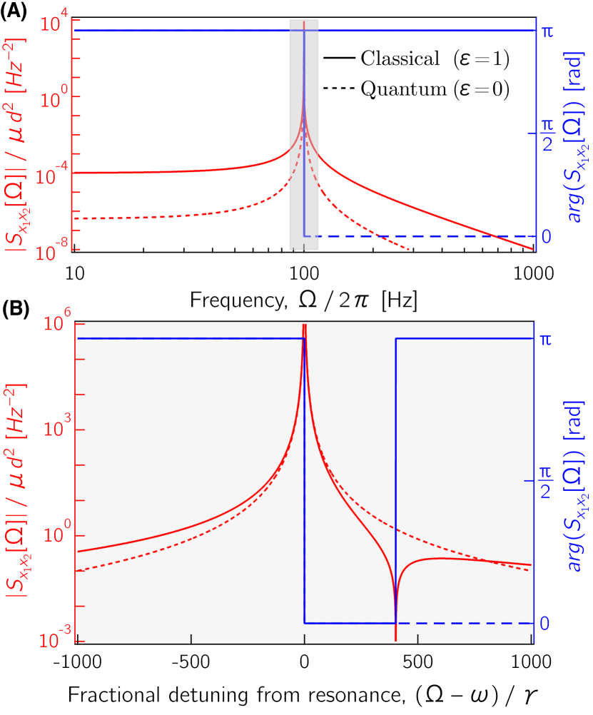
Figure 1: Cross-correlation of the motion of a pair of quantum oscillators mediated by stochastic classical gravity. Here the label “Quantum” corresponds to setting $\epsilon=0$, in which case, gravity is a quantum field; “Classical” corresponds to $\epsilon=1$. The two oscillators are identical with resonance frequency $\omega=2\pi\cdot 100\,\mathrm{{Hz}}$, and damping rate $\gamma=2\pi\cdot 10^{-3}\,\mathrm{{Hz}}$. The red traces depict $\absolutevalue{S_{x_{1}x_{2}}}$ while blue depicts the phase $\arg S_{x_{1}x_{2}}$. The effect of the gravitational Lindbladian is an increase in the noise, by a factor $\omega/2\gamma(2\bar{N}+1)$ compared to the quantum case, and an additional $\pi$ phase shift at a detuning $\Delta\Omega\approx 2\gamma(2\bar{N}+1)$ from resonance.

Experimental signature. We now consider an experimentally relevant example where two massive quantum harmonic oscillators interact with each other via classical gravity. As we will show, their motion is correlated via the classical stochastic gravitational field mediating their interaction, and these correlations offer a qualitatively distinct prediction from one where gravity is assumed quantum (i.e. $\epsilon=0$).

We take the masses to be one-dimensional quantum harmonic oscillators of frequency $\omega_{1,2}$ each coupled to independent thermal baths of occupation $\bar{N}_{1,2}$ at rates $\gamma_{1,2}$. They are also gravitationally coupled to each other by their close proximity of distance $R$. This scenario is described by the equation

$$\dot{\rho}_{Q}(t)=-\frac{i}{\hbar}[\hat{H}_{\mathrm{{eff}}},\hat{\rho}_{Q}]+\mathcal{L}\left[\hat{\rho}_{Q}\right],$$ (10)

where $\hat{H}_{\mathrm{{eff}}}=\hat{H}_{Q}+\hat{H}_{G}$, with $\hat{H}_{Q}=\sum_{i}\hbar\omega_{i}(\hat{a}_{i}^{\dagger}\hat{a}_{i}+\tfrac{1}{2})$, and $\mathcal{L}=\mathcal{L}_{G}+\sum_{i}\mathcal{L}_{i}$, where $\mathcal{L}_{i}[\hat{\rho}_{Q}]=\gamma_{i}(\bar{N}_{i}+1)(\hat{a}_{i}\hat{\rho}_{Q}\hat{a}^{\dagger}_{i}-\tfrac{1}{2}[\hat{a}_{i}^{\dagger}\hat{a}_{i},\hat{\rho}_{Q}]_{+})+\gamma_{i}\bar{N}_{i}(\hat{a}^{\dagger}_{i}\hat{\rho}_{Q}\hat{a}_{i}-\tfrac{1}{2}[\hat{a}_{i}\hat{a}^{\dagger}_{i},\hat{\rho}_{Q}]_{+})$, describes the realistic coupling of any experimental source mass to a thermal bath of average thermal occupation $\bar{N}_{i}$ [45]. Here the gravitational interaction Hamiltonian $\hat{H}_{G}\approx Gm_{1}m_{2}\hat{x}_{1}\hat{x}_{2}/(2R^{3})$ is obtained from the mass density $\hat{f}(x)=m_{1}\delta(x+\tfrac{R}{2}-\hat{x}_{1})+m_{2}\delta(x-\tfrac{R}{2}-\hat{x}_{2})$ to evaluating Eq. 7 by first performing a small-distance expansion of the Coulombic denominator, and then performing the integrals. (Note that here we have dropped a singular self-interaction term whose origin is the point-mass approximation of the center-of-mass degree of freedom of the oscillator; for an oscillator that is formed of an elastic continuum, these terms will excite internal modes.)

The primary effect of the gravitational interaction is the correlation developed via the gravity Lindbladian $\mathcal{L}_{G}$. The simplest experimentally accessible observable sensitive to non-zero value of $\epsilon$ is the the cross-correlation of the quantized displacements $\hat{x}_{1,2}$ of the two gravitating oscillators. This can be inferred from the outcomes of continuous measurements of the displacements, say by interferometric displacement measurements. (These measurement schemes cause back-action [46] whose effect is an increased apparent temperature [47, 48], which can thus be absorbed into the bath occupations $\bar{N}_{i}$; back-action-evasion measurements may also be imagined [49, 50, 51].) The theory presented above can produce a concrete prediction for the cross-correlation spectrum of the displacement $S_{x_{1}x_{2}}[\Omega]$. We do so by first mapping the master equation [Eq. 10] into a partial differential equation (PDE) for the characteristic function $\chi(\mathbf{\xi},\mathbf{\xi}^{*},t)=\Tr[\hat{\rho}_{Q}(t)\hat{D}(\mathbf{\xi})]$, where $\hat{D}(\xi)=\prod_{i}\exp[\xi_{i}\hat{a}_{i}^{\dagger}-\xi_{i}^{*}\hat{a}_{i}]$ are a set of complete orthogonal basis in the set of operators of the joint Hilbert space of the two oscillators [52]. Since the resulting PDE is of second order, and the initial thermal state of the oscillators is Gaussian in $\chi(\xi,\xi^{*},0)$, a Gaussian ansatz suffices to solve for $\chi(\xi,\xi^{*},t)$. From this solution, we obtain equal-time correlations of the coordinates and momenta of the oscillators. Finally, employing the quantum regression theorem [45], we get the unequal-time correlations, whose Fourier transform gives the cross-correlation spectrum (see Section E.2 for the gory details). For identical oscillators, the result is (Section E.3 contains the full expressions)

$$S_{x_{1}x_{2}}[\Omega]\approx-\mu\left(\frac{d}{\omega}\right)^{2}\begin{dcases}\epsilon+\frac{2\bar{N}+1}{Q};&\Omega\ll\omega\\ \left(\frac{\omega}{\Omega}\right)^{4}\left(\epsilon-\frac{2\bar{N}+1}{Q}\right);&\Omega\gg\omega,\end{dcases}$$ (11)

where, $Q=\omega/(2\gamma)$ is the quality factor of the oscillator, and $\mu=(2G/R^{3})(m/\omega)$. Importantly, gravitationally interacting oscillators with quality factor $Q\gtrsim\bar{N}/\epsilon$ can be sensitive probes of whether $\epsilon$ is zero or not.

Figure 1 depicts the cross-correlation $S_{x_{1}x_{2}}$ for a typical scenario of two identical mechanical oscillators coupled via gravity, under the hypothesis that gravity is quantum ($\epsilon=0$) or that it is a classical stochastic field, with $\epsilon=1$ chosen arbitrarily. In the quantum case, the correlation between the two oscillators is purely via the quantized Newtonian interaction Hamiltonian $\hat{H}_{G}$, resulting in correlated motion across all frequencies, with most of the motion concentrated around the common resonance. In the classical stochastic case, the joint interaction mediated by $\mathcal{L}_{G}$ apparently produces anti-correlated motion away from resonance, accompanied by a characteristic phase shift $\arg S_{x_{1}x_{2}}$. This phase shift persists for all non-zero values of $\epsilon$ (unlike the anti-correlated feature in $\absolutevalue{S_{x_{1}x_{2}}}$, which can diminish with $\epsilon$) and is thus a robust experimental signature that gravity is classical. Thus, careful measurements of the cross-correlation of two gravitationally coupled highly coherent mechanical oscillators can distinguish between the hypothesis that gravity is classical or quantum.

Conclusion. We have derived a natural and pathology-free theory of two quantized bodies interacting via classical gravity, and produced an experimentally testable implication of this theory that can distinguish whether gravity is classical or not. Testing this prediction calls for an experiment where two highly coherent massive oscillators are coupled to each other via gravity. Importantly, they do not need to be in superposition states [26, 27]. Further, the experimental signatures are distinct from the effects of extraneous decoherence.

Although it is only the Newtonian limit of a stochastic classical gravitational interaction that has been explicated here, the more fundamental question of producing a fully covariant generalization, or indeed, whether such a version is sensible, is outstanding. Equation 1 can conceivably be generalized to spacetimes foliated by spacelike surfaces, since the extension from the case of a fixed time coordinate to a general timelike coordinate is straightforward [53]. Any further generalization — for example, to elucidate the correct modification of general relativity beyond the semi-classical approximation, as achieved by Eq. 5 for the Newtonian limit — will require a conceptual leap.

Appendix A Consistency with classical stochastic dynamics

In this section we aim to match the full quantum-classical equation with the reduced stochastic dynamics of the system. We consider the general equation [Eq. 1 of the main text]

$$\begin{split}\dot{\hat{\rho}}_{t}=&-\frac{i}{\hbar}[\hat{H}_{t},\hat{\rho}_{t}]+Q_{\alpha\beta}\left(\hat{L}_{\alpha}\hat{\rho}_{t}\hat{L}_{\beta}^{\dagger}-\frac{1}{2}[\hat{L}_{\beta}^{\dagger}\hat{L}_{\alpha},\hat{\rho}_{t}]_{+}\right)\\ &+\partial_{z_{i}}\left(C_{i}\hat{\rho}_{t}\right)+\partial_{z_{i}z_{j}}\left(C_{ij}\hat{\rho}_{t}\right)\\ &+\partial_{z_{i}}\left(M_{\alpha i}\hat{\rho}_{t}\hat{L}^{\dagger}_{\alpha}+\mathrm{h.c.}\right).\end{split}$$ (12)

and try to understand the behavior of the classical subsystem that is described by $p_{t}=\Tr\hat{\rho}_{t}$. For this we need to take the trace on both sides of Eq. 12 and match it to the equation of motion that will be a natural assumption of the evolution of $p_{t}$. Below we give a motivation of the form of this equation.

A.1 Motivation for the classical subsystem equation

Let’s consider a master equation for two classical systems that interact with each other and have a second order diffusion. Let’s assume that the Hamiltonian of the system is given by $H(z_{i(1)},z_{i(2)})=H_{1}(z_{i(1)})+H_{2}(z_{i(2)})+H_{I}(z_{i(1)},z_{i(2)})$, where $z_{i(1)}$ and $z_{i(2)}$ are the degrees of freedom that correspond to the first and the second systems respectively. Let’s define the joint probability as $p(z_{i(1),z_{i(2)}})$. Then, a natural choice of the equation of motion for the joint system is

$$\dot{p}=\partial_{z_{i(1)}}(C_{i(1)}p)+\partial_{z_{i(2)}}(C_{i(2)}p)+\\ +\partial_{z_{i(1)}z_{j(1)}}(C_{ij(1,1)}p)+\partial_{z_{i(2)}z_{j(2)}}(C_{ij(2,2)}p)+\\ +\partial_{z_{i(1)}z_{j(2)}}(C_{ij(1,2)}p).$$ (13)

The first line describes the conservative evolution of two systems, the second line describes the diffusive evolution of both of the systems, and the third line describes the mutual diffusion of both of the system. Let’s assume that we are interested only in effective evolution of system 1. Probability for system 1 is

$$p_{1}(z_{i(1)})=\int dz_{i(2)}\;p(z_{i(1)},z_{i(2)}).$$ (14)

With that we split the full probability of the system $p(z_{i(1)},z_{i(2)})$ into the probability distribution of $p_{1}(z_{i(1)})$ and a conditional probability of the second system $\tilde{p}_{2}(z_{i(1)},z_{i(2)})$:

$$p(z_{i(1)},z_{i(2)})=p_{1}(z_{i(1)})\;\tilde{p}_{2}(z_{i(1)},z_{i(2)}).$$ (15)

By definition of conditional probability,

$$\int dz_{(2)}\;\tilde{p}_{2}(z_{i(1)},z_{i(2)})=1.$$ (16)

Now let’s assume that $C_{i(1)}=C_{i}(z_{i(1)})+C_{I,i}(z_{i(1)},z_{i(2)})$ – coefficients that describe the evolution of system 1 and interaction of systems 1 and 2. Integrating Eq. 13 over $z_{i(2)}$, we obtain

$$\dot{p}_{1}=\partial_{z_{i}}(C_{i}p_{1})+\partial_{z_{i}z_{j}}(C_{ij}p_{1})+\partial_{z_{i}}(\langle C_{I,i}\rangle p_{1}),$$ (17)

where we introduced simplified notation $z_{i}=z_{i(1)}$, $C_{ij(1,1)}=C_{ij}$ and

$$\langle C_{I,i}\rangle(z_{i})=\int dz_{2}C_{I,i}(z_{i},z_{i(2)})\tilde{p}_{2}(z_{i},z_{i(2)}).$$ (18)

As we can see, the only trace of the second system remained in the equation of motion for system 1 are coefficients $\langle C_{I,i}\rangle$ that know about the evolution of system two through $\tilde{p}_{2}$. Now, let’s assume that system 1 is a classical gravity field and system 2 is a set of classical masses that can be subjects to forces besides the gravity. The interaction Hamiltonian for such a system is

$$H_{I}=\int\differential^{3}x\Phi(x)f(x),$$ (19)

where $f(x)$ is the mass density function for the system of masses. Comparing the expression that comes from $\{H_{I},p\}$ to $\partial_{z_{i}}(C_{I,i}p_{1})$ terms gives

$$C_{I,\Pi(x)}=\int dz_{2}f(x)\tilde{p}_{2}(z_{1},z_{2});\quad C_{I,\Phi(x)}=0.$$ (20)

The $\Pi(x)$ is a conjugate momentum to $\Phi(x)$. Therefore, the coefficients in the case of this interaction Hamiltonian are just mass expectation values over the ensemble of masses for a fixed configuration of gravity fields. Therefore, one could assume a similar expression for the case when the system of masses is quantum. However, now the averaged mass density is given by

$$C_{I,\Pi(x)}=\Tr[\hat{\tilde{\rho}}_{t}\,\hat{f}(x)],$$ (21)

where $\hat{\rho}_{t}=\hat{\tilde{\rho}}_{t}\,p_{t}$.

Based on the above consideration, we insist that the classical state, $p_{t}(z)\equiv\Tr\hat{\rho}_{t}(z)$, satisfy a stochastic Liouville equation

$$\begin{split}\dot{p}_{t}&=\left\{H_{C},p_{t}\right\}+\partial_{z_{i}z_{j}}\left(D_{ij}p_{t}\right)+\partial_{\Pi(x)}(C_{I,\Pi(x)}(x)p_{t})\\ \end{split}$$ (22)

where $H$ is a classical Hamiltonian, $\{\cdot,\cdot\}$ is the Poisson bracket, and $D$ is some diffusion constant.

Taking the trace of Eq. 12, the first line vanishes, while the second gives $\partial_{z_{i}}(C_{i}p)+\partial_{z_{i}z_{j}}(C_{ij}p)$. The second term is the classical diffusion assumed in Eq. 23, with $D_{ij}=C_{ij}$. The third line, in it’s turn, gives $\partial_{z_{i}}(M_{\alpha i}\langle\hat{L}_{\alpha}^{\dagger}\rangle+\mathrm{c.c.})$ The first term subsumes the Poisson bracket if we notice that, $\{H,p\}=(\partial_{z_{i}}H)J_{ij}(\partial_{z_{j}}p)$ (here $J$ is the symplectic matrix), which is identical to $\partial_{z_{i}}(C_{i}p)$ if $\partial_{z_{i}}(C_{i})=0$ and $C_{j}+(\partial_{z_{i}}H)J_{ij}=0$. (The skew-symmetry of $J$ ensures the consistency of these conditions.)

The trace of the third line of Eq. 12 gives $\partial_{z_{i}}(M_{\alpha i}\langle L_{\alpha}^{\dagger}\rangle+\mathrm{c.c.})$ and has to be compared to the third term in the Eq. 23. Assuming that the equations of motion have to be true for all states of quantum matter, some of the jump operators $\hat{L}_{\alpha}$ have to correspond to $\hat{f}(x_{\alpha})$, and the coefficients $M_{\alpha i}$ should correspond to the coefficients $C_{I,i}(x_{\alpha})=\real M_{\alpha i}$. This means that for those terms the bracket can be reconstructed and the “quantum-classical diffusion” term is responsible for mediating the term of the form $\{\hat{H}_{I},\hat{\rho}_{t}\}$ and similar. However, with this consideration we can only fix the form of the first and third terms Liouville Eq. 23:

$$\begin{split}\dot{p}_{t}&=\left\{H_{C},p_{t}\right\}+\Tr\left\{\hat{H}_{I},\hat{\rho}_{t}\right\}+\partial_{z_{i}z_{j}}\left(D_{ij}p_{t}\right),\\ \end{split}$$ (23)

and the quantum structure of such term in Eq. 12 is partially lost in taking the trace.

A.2 Symplectic structure

One can approach the same problem from a different side. We notice that the terms that contain $M_{\alpha i}$ are of the first order dynamics form in the classical part of the system, and therefore are similar to the $C_{i}$ terms . The notion of integrability for the $C_{i}$ terms grounds on the presence of symplectic structure in the classical phase space and the fact that the coefficients $C_{i}$ satisfy the integrability conditions

$$\partial_{z_{i}}C_{i}=0,\quad C_{j}+(\partial_{z_{i}}H_{C})J_{ij}=0.$$ (24)

If we assume that conditions of similar form apply to $M_{\alpha i}$

$$\partial_{z_{i}}M_{\alpha i}=0;\quad M_{\alpha j}+(\partial_{z_{i}}h_{\alpha})J_{ij}=0,$$ (25)

then one can reconstruct the Poisson bracket for the quantum-classical diffusion term, since the conditions in Eq. 25 are necessary and sufficient. To obtain the equation of interest for $p_{t}$ we first take the $\Tr$ of Eq. 12, which gives

$$\dot{p}_{t}=\partial_{z_{i}}(C_{i}p_{t})+\partial_{z_{i}z_{j}}(C_{ij}p_{t})+\Tr\partial_{z_{i}}(M_{\alpha i}\hat{\rho}_{t}L_{\alpha}^{\dagger}+\mathrm{h.c.})$$ (26)

With the use of Eq. 24 the first term then can be rewritten as

$$\partial_{z_{i}}(C_{i}p_{t})=\{H_{C},p_{t}\}.$$ (27)

The third term using Eq. 25 becomes

$$\Tr\partial_{z_{i}}(M_{\alpha i}\hat{\rho}_{t}L_{\alpha}^{\dagger}+\mathrm{h.c.})=\Tr{\hat{H}_{I},\hat{\rho}_{t}},$$ (28)

where $\hat{H}_{I}=h_{\alpha}\hat{L}_{\alpha}^{\dagger}+h_{\alpha}^{*}\hat{L}_{\alpha}$. Therefore, the resulting equation becomes

$$\begin{split}\dot{p}_{t}&=\left\{H_{C},p_{t}\right\}+\Tr\left\{\hat{H}_{I},\hat{\rho}_{t}\right\}+\partial_{z_{i}z_{j}}\left(D_{ij}p_{t}\right).\\ \end{split}$$ (29)

Appendix B Recovering a full quantum structure

In order to recover the full quantum structure of the quantum-classical diffusion term in Eq. 12, we deal with the last term in Eq. 12 separately, we rewrite

$$\begin{split}M_{\alpha i}\hat{\rho}_{t}\hat{L}^{\dagger}_{\alpha}+\mathrm{{h.c.}}=&\left[\hat{\rho}_{t},\tfrac{1}{2}(M_{\alpha i}\hat{L}_{\alpha}^{\dagger}-\mathrm{{h.c.}})\right]\\ +&\left[\hat{\rho}_{t},\tfrac{1}{2}(M_{\alpha i}\hat{L}_{\alpha}^{\dagger}+\mathrm{{h.c.}})\right]_{+}.\end{split}$$ (30)

Inserting this in Eq. 12 and computing its trace of Eq. 12 shows that the last term has to take a form Eq. 30 is:

$$\partial_{z_{i}}\left[\hat{\rho}_{t},\tfrac{1}{2}(M_{\alpha i}\hat{L}_{\alpha}^{\dagger}+\mathrm{{h.c.}})\right]_{+}=\mathrm{{Herm}}\left\{H_{I}(z,t),\hat{\rho}_{t}\right\}.$$ (31)

Here $\mathrm{{Herm}}$ corresponds to the Hermitian part of the operator, curly bracket corresponds to the Poisson bracket. However the comparison of the first term on the right hand side of Eq. 30 would yield no constraints, since the trace of it over the quantum part is 0 due to the presence of commutator. Moreover, the terms inside the commutator are linearly independent from the terms in the anti-commutator. Even though there is no reason for the commutator term in Eq. 30 to be described by a single function, we assume so in order to ensure the theory is described by a finitely. That is, we assume the first term in Eq. 30 is related to a function $iH^{\prime}$ (with $H^{\prime}$ hermitian) via a Poisson bracket as

$$\partial_{z_{i}}\left[\hat{\rho}_{t},\tfrac{1}{2}(M_{\alpha i}\hat{L}_{\alpha}^{\dagger}-\mathrm{{h.c.}})\right]_{-}=i\,\mathrm{{AntiHerm}}\left\{H^{\prime}(z,t),\hat{\rho}_{t}\right\},$$ (32)

where $\mathrm{{AntiHerm}}$ means the anti-hermitian part of the the expression.

Thus Eq. 12 becomes

$$\begin{split}\dot{\hat{\rho}}_{t}=&-\frac{i}{\hbar}[\hat{H},\hat{\rho}_{t}]+\,Q_{\alpha\beta}\left(\hat{L}_{\alpha}\hat{\rho}_{t}\hat{L}_{\beta}^{\dagger}-\frac{1}{2}[\hat{L}_{\beta}^{\dagger}\hat{L}_{\alpha},\hat{\rho}_{t}]_{+}\right)\\ &+\mathrm{{Herm}}\left\{\hat{H},\hat{\rho}_{t}\right\}+i\,\mathrm{{AntiHerm}}\left\{\hat{H}^{\prime},\hat{\rho}_{t}\right\}\\ &+\partial_{z_{i}z_{j}}\left(C_{ij}\hat{\rho}_{t}\right).\end{split}$$ (33)

Appendix C Hamiltonian in the Newtonian limit of general relativity

In the following we describe the construction of the Hamiltonian of the gravitational field in the Newtonian limit of general relativity.

We linearize the metric $g$ as

$$g_{\mu\nu}=\eta_{\mu\nu}+h_{\mu\nu},\quad|h_{\mu\nu}|\ll 1,$$ (34)

where $\eta_{\mu\nu}=\mathrm{{diag}}(-1,+1,+1,+1)$. The non-uniqueness of the above decomposition is encoded in the gauge symmetry [54, §7.1]

$$h_{\mu\nu}\rightarrow h_{\mu\nu}+\partial_{\mu}\xi_{\nu}+\partial_{\nu}\xi_{\mu}.$$ (35)

Adopting the parametrization

$$h_{00} =-2\Phi$$

$$h_{0i} =w_{i}$$

$$h_{ij} =2s_{ij}-2\Psi\delta_{ij},$$

where $s_{ij}$ is traceless, the gauge symmetry is equivalent to the transformations

$$\begin{split}\Phi&\rightarrow\tilde{\Phi}=\Phi+\partial_{0}\xi_{0}\\ \Psi&\rightarrow\tilde{\Psi}=\Psi-\tfrac{1}{3}\partial_{i}\xi^{i}\\ w_{i}&\rightarrow\tilde{w}_{i}=w_{i}+\partial_{0}\xi^{i}-\partial_{i}\xi^{0}\\ s_{ij}&\rightarrow\tilde{s}_{ij}=s_{ij}+\partial_{(i}\xi_{j)}-\tfrac{1}{3}\delta_{ij}\partial_{k}\xi^{k}.\end{split}$$ (36)

By direct manipulation of the geodesic equation, it can be verified that the dynamics of particle three-momenta $\pi^{i}$ in the field is

$$\dot{\pi}^{i}\approx-E\left[\partial_{i}\Phi+\partial_{0}w_{i}+O\left(\tfrac{v^{i}}{c}\right)\right],$$ (37)

where $E$ is its energy. First, this means that $\Phi$ can be interpreted as the (Newtonian) potential. Secondly, since every time derivative comes with an additional factor of $1/c$, any gauge transformation of $\Phi$ and $w_{i}$ will only have an impact on Eq. 37 only in the order of $1/c$, and so, in the low energy limit the Newtonian potential is well-defined and gauge-invariant.

Our aim is to construct a Hamiltonian description of the Newtonian potential $\Phi$. It is possible to do this without having to deal with the full canonical theory of general relativity [40, 41]. The idea is to first identify a gauge in which the Newtonian potential is the only relevant degree of freedom, and then apply the canonical formalism with these gauge conditions as Lagrangian constraints.

We first identify the required gauge. Consider the equations for components of Einstein tensor $G_{00}$ and $G^{i}_{i}$:

$$G_{00} =2\nabla^{2}\Psi+\partial_{k}\partial_{l}s^{kl},$$

$$G^{i}_{i} =2\nabla^{2}\left(\Phi-\Psi\right)+4\partial_{0}\partial_{k}w^{k}+6\partial_{0}^{2}\Psi-\partial_{k}\partial_{l}s^{kl}.$$

Eliminating $\partial_{k}\partial_{l}s^{kl}$ gives

$$G^{i}_{i}=2\nabla^{2}\Phi+4\partial_{0}\partial_{k}w^{k}+6\partial_{0}^{2}\Psi-G_{00}.$$ (38)

Using this, the equation of motion, $G_{\mu\nu}=8\pi GT_{\mu\nu}$, becomes

$$G_{00}=8\pi GT_{00},\qquad G^{i}_{i}=8\pi GT^{i}_{i}.$$ (39)

Eliminating $G_{00}$ between Eqs. 38 and 39:

$$(\nabla^{2}\Phi-\partial_{0}^{2}\Psi)+2\partial_{0}(\partial_{k}w^{k}+2\partial_{0}\Psi)=4\pi G\left(T_{00}+T^{i}_{i}\right).$$ (40)

This almost has the form of the field equation of the massless scalar field $\Phi$, if only $\Phi=\Psi$, and the extraneous terms on the left-hand side can be eliminated.

Both these goals can be met by proper choice of gauge. That is, we demand that

$$\tilde{\Phi}=\tilde{\Psi},\quad\partial_{k}\tilde{w}^{k}+2\partial_{0}\tilde{\Psi}=0,$$ (41)

Using the gauge equations [Eq. 36], this is tantamount to $\xi^{\mu}$ satisfying

$$\begin{split}\partial_{0}\xi^{0}+\frac{1}{3}\partial_{i}\xi^{i}&=\Phi-\Psi\\ 2\partial_{0}^{2}\xi^{0}-\partial_{0}\partial_{i}\xi^{i}+\nabla^{2}\xi^{0}&=2\partial_{0}\Phi+\partial_{k}w^{k}.\end{split}$$ (42)

It is clear that these equations have a solution $\xi^{\mu}$ for given differentiable fields $(\Phi,\Psi,w^{k})$. Imposing the gauge constraints in Eq. 41 in the equation of motion [Eq. 40] gives

$$\nabla^{2}\tilde{\Phi}-\partial_{0}^{2}\tilde{\Phi}=4\pi G\left(T_{00}+T^{i}_{i}\right).$$ (43)

Notice that since $T^{i}_{i}$ is of order $1/c^{2}$, it is negligible compared to $T_{00}$. Then it is clear that this equation can arise from the Hamiltonian of a massless scalar field coupled to $T_{00}=f$, the mass density.

Formally, we can construct the Hamiltonian for $\Phi$ by considering the Lagrangian density $\mathcal{L}[h]$ of linearized gravity with the gauge conditions inserted with Lagrange multiplier $\lambda$. The terms that have $\Phi$ in the density are:

$$\mathcal{L}\supset\frac{1}{2}\eta^{\mu\nu}(\partial_{\mu}\Phi)(\partial_{\nu}\Phi)-4\pi G\left(T_{00}+T^{i}_{i}\right)\Phi-\\ -2\eta^{\mu\nu}(\partial_{\mu}s_{ii})(\partial_{\nu}\Phi)+8\left(\left(\partial_{0}\Phi\right)^{2}+(\partial_{0}\Phi)(\partial_{k}w^{k})\right)+\\ +\lambda\left(2\partial_{0}\Phi+\partial_{k}w^{k}\right)$$ (44)

Euler-Lagrange equation for $\Phi$ will result just in Eq. 43 when all the constraints are applied. Notice that the Lagrangian is at most quadratic in $\partial_{0}\Phi$, therefore the Hamiltonian will be quadratic in $\Phi$ and its conjugate momentum $\Pi=\dot{\Phi}$. To retrieve the Hamiltonian with only $\Phi$ and $\Pi$ degrees of freedom, we take the adiabatic limit in two steps. At the first step, we take $w_{k}\rightarrow 0$, $s_{ij}\rightarrow 0$, $T_{0i}\rightarrow 0$, $T_{ij}\rightarrow 0$ since these degrees of freedom are of the order of $1/c$. This limit will result in the Hamiltonian, whose normalized form is

$$H_{G}=\int\differential^{3}x\left[2\pi Gc^{2}\Pi^{2}+\frac{|\nabla\Phi|^{2}}{8\pi G}-\Phi f(x)\right].$$ (45)

Appendix D Modified quantum Newton’s Law

We here derive the modified version of Newton’s law from the equation of motion for $\hat{\rho}_{t}(z)$

$$\begin{split}\dot{\hat{\rho}}_{t}&=-\frac{i}{\hbar}[\hat{H},\hat{\rho}_{t}]+\,Q_{\alpha\beta}\left(\hat{L}_{\alpha}\hat{\rho}_{t}\hat{L}_{\beta}^{\dagger}-\frac{1}{2}[\hat{L}_{\beta}^{\dagger}\hat{L}_{\alpha},\hat{\rho}_{t}]_{+}\right)+\\ +\;&\mathrm{{Herm}}\left\{\hat{H},\hat{\rho}_{t}\right\}+i\,\mathrm{{AntiHerm}}\left\{\hat{H}^{\prime},\hat{\rho}_{t}\right\}+\partial_{z_{i}z_{j}}\left(C_{ij}\hat{\rho}_{t}\right).\end{split}$$ (46)

where the Hamiltonian

$$\hat{H}(z)=\hat{H}_{Q}+\int\differential^{3}x\left[2\pi Gc^{2}\Pi^{2}+\frac{|\nabla\Phi|^{2}}{8\pi G}-\Phi\hat{f}(x)\right],$$ (47)

depends on the phase space variables of the classical system $z=(\Phi,\Pi)$, and,

$$\hat{H}^{\prime}(z)=-\epsilon\int\differential^{3}x\;\Phi(x)\hat{f}(x).$$ (48)

In order to reduce Eq. 46 to an equation closed in $\hat{\rho}_{Q}$, we need to integrate out $z$. As argued in the main text, in case of weak gravity it suffices to consider the diffusion coefficients to zeroth order in $z$. Then integrating Eq. 46 gives

$$\begin{split}\dot{\hat{\rho}}_{Q}=&-\frac{i}{\hbar}\int\differential{z}\,[\hat{H},\hat{\rho}_{t}]\\ &+\int\differential{z}\,\mathrm{{Herm}}\left\{\hat{H},\hat{\rho}_{t}\right\}\\ &+i\int\differential{z}\,\mathrm{{AntiHerm}}\left\{\hat{H}^{\prime},\hat{\rho}_{t}\right\}\\ &+Q_{\alpha\beta}\left(\hat{L}_{\alpha}\hat{\rho}_{Q}\hat{L}_{\beta}^{\dagger}-\frac{1}{2}\left[\hat{L}_{\alpha}^{\dagger}\hat{L}_{\beta},\hat{\rho}_{Q}\right]_{+}\right);\end{split}$$ (49)

note that the classical diffusion term has disappeared by integrating it by parts and assuming the state $\hat{\rho}(z\rightarrow\infty)\rightarrow 0$. It is straightforward to verify that the Poisson bracket terms (Herm and AntiHerm), after substitution of the Hamiltonians, also integrates by parts to zero. The only remaining term is:

$$\begin{split}\int\differential{z}[\hat{H}(z,t),\hat{\rho}(z)]=\int\differential^{3}x\left[\hat{f}(x),\left\langle{\Phi(x)}\right\rangle_{Q}\right].\end{split}$$ (50)

Here we use the notation $\left\langle{O}\right\rangle_{Q}\equiv\int\differential{z}O\hat{\rho}_{t}(z)$.

To simplify the RHS of Eq. 50, we need to compute the evolution of $\left<\Phi(x)\right>_{Q}$. For this we compute the equations of motion of $\left<\Phi(x)\right>_{Q}$ and $\left<\Pi(x)\right>_{Q}$ by multiplying Eq. 46 by $\Phi(x)$ and $\Pi(x)$ respectively and integrating over $z$. These equations are

$$\begin{split}4\pi Gc^{2}\left\langle{\Pi(x)}\right\rangle_{Q}&=\partial_{t}\left\langle{\Phi(x)}\right\rangle_{Q}+i[\hat{H}_{Q},\left\langle{\Phi(x)}\right\rangle_{Q}]\\ &\qquad+i\int\differential^{3}x^{\prime}\left[\hat{f}(x^{\prime}),\left\langle{\Phi(x)\Phi(x^{\prime})}\right\rangle_{Q}\right]\\ &\qquad-Q^{\alpha\beta}\left(\hat{L}_{\alpha}\left\langle{\Phi(x)}\right\rangle_{Q}\hat{L}_{\beta}^{\dagger}-\frac{1}{2}\left[\hat{L}_{\beta}^{\dagger}\hat{L}_{\alpha},\left\langle{\Phi(x)}\right\rangle_{Q}\right]_{+}\right),\\ \frac{1}{4\pi G}\left\langle{\nabla^{2}\Phi(x)}\right\rangle_{Q}&=-\mathrm{{Herm}}\left(\hat{f}(x)\hat{\rho}_{Q}\right)-i\epsilon\,\mathrm{{AntiHerm}}\left(\hat{f}(x)\hat{\rho}_{Q}\right)\\ &\qquad+\partial_{t}\left\langle{\Pi(x)}\right\rangle_{Q}+i[\hat{H}_{Q},\left\langle{\Pi(x)}\right\rangle_{Q}]\\ &\qquad+i\int\differential^{3}x^{\prime}\left[\hat{f}(x^{\prime}),\left\langle{\Pi(x)\Phi(x^{\prime})}\right\rangle_{Q}\right]\\ &\qquad-Q^{\alpha\beta}\left(\hat{L}_{\alpha}\left\langle{\Pi(x)}\right\rangle_{Q}\hat{L}_{\beta}^{\dagger}-\frac{1}{2}\left[L_{\beta}^{\dagger}L_{\alpha},\left\langle{\Pi(x)}\right\rangle_{Q}\right]_{+}\right).\end{split}$$

Mercifully, in the adiabatic limit ($c\rightarrow\infty$), these collapse to

$$\left\langle{\Pi(x)}\right\rangle_{Q} =0,$$

$$\frac{\left\langle{\Phi(x)}\right\rangle_{Q}}{4\pi G} =-\frac{1}{2}\left(\hat{f}(x)\hat{\rho}_{Q}+\hat{\rho}_{Q}\hat{f}(x)\right)-i\epsilon\frac{1}{2}\left(\hat{f}(x)\hat{\rho}_{Q}-\hat{\rho}_{Q}\hat{f}(x)\right),$$

so that

$$\left\langle{\Phi(x)}\right\rangle_{Q}=-G\int\frac{\differential^{3}x^{\prime}}{|x-x^{\prime}|}\left[\frac{1}{2}\left(\hat{f}(x)\hat{\rho}_{Q}+\hat{\rho}_{Q}\hat{f}(x)\right)+i\epsilon\frac{1}{2}\left(\hat{f}(x)\hat{\rho}_{Q}-\hat{\rho}_{Q}\hat{f}(x)\right)\right].$$ (51)

Substituting Eq. 51 into Eq. 50 and grouping terms gives the closed equation of motion for $\hat{\rho}_{Q}$:

$$\begin{split}\dot{\hat{\rho}}_{Q}=&-\frac{i}{\hbar}[\hat{H}_{\mathrm{{eff}}},\hat{\rho}_{Q}]\\ &-\epsilon\frac{G}{2}\int\frac{\differential^{3}x\,\differential^{3}x^{\prime}}{|x-x^{\prime}|}\left[\hat{f}(x),\left[\hat{f}(x^{\prime}),\rho_{Q}\right]\right]\\ &+Q_{\alpha\beta}\left(\hat{L}_{\alpha}\hat{\rho}_{Q}\hat{L}_{\beta}^{\dagger}-\frac{1}{2}\left[\hat{L}_{\alpha}^{\dagger}\hat{L}_{\beta},\hat{\rho}_{Q}\right]_{+}\right),\end{split}$$ (52)

where the effective Hamiltonian is

$$\hat{H}_{\mathrm{{eff}}}=\hat{H}_{Q}-\frac{G}{2}\int\differential^{3}x\,\differential^{3}x^{\prime}\frac{\hat{f}(x)\hat{f}(x^{\prime})}{|x-x^{\prime}|},$$ (53)

as it was claimed in the main text. Further, Eq. 52 has picked up a gravity-dependent Lindblad term.

Appendix E Gravity-induced correlation between two oscillators

We are interested in the correlation between the oscillators’ positions $\hat{x}_{1}$, $\hat{x}_{2}$ and momenta $\hat{p}_{1}$, $\hat{p}_{2}$, while they interact with each other through gravity, and in the presence of thermal decoherence. As a measure of the correlations, we will choose the symmetrized power spectral density (PSD) of the observables, defined by

$$S_{\hat{A}_{i}\hat{A}_{j}}[\Omega]=\int\limits_{-\infty}^{+\infty}\left\langle{\tfrac{1}{2}[\hat{A}_{i}(0),\hat{A}_{j}(t)]_{+}}\right\rangle e^{-i\Omega t}\differential{t}.$$ (54)

Suppose the expectation values $\langle\hat{A}_{i}\rangle$ satisfy a closed system of equations

$$\partial_{t}\langle\hat{A}_{i}(t)\rangle=K_{ij}\langle\hat{A}_{j}(t)\rangle,$$ (55)

then the quantum regression theorem [45] asserts that the unequal-time correlations satisfy

$$\partial_{t}\langle\hat{A}_{i}(t)\hat{A}_{k}(0)\rangle=K_{ij}\langle\hat{A}_{j}(t)\hat{A}_{k}(0)\rangle.$$ (56)

These can be solved if the initial conditions, the equal-time correlations $\langle\hat{A}_{i}(0)\hat{A}_{k}(0)\rangle$, are specified. Then performing a one-sided Fourier transform (i.e. on positive time) solves Eq. 56, and allows us to compute the one-sided PSD (i.e. PSD defined similar to Eq. 54 but with integration over positive time):

$$S_{A_{i}A_{j}}^{+}[\Omega]=\sum_{k}\left\langle\tfrac{1}{2}[\hat{A}_{i}(0),\hat{A}_{k}(0)]_{+}\right\rangle\left[(i\Omega-K^{T})^{-1}\right]_{kj}.$$ (57)

Assuming weak-stationarity of the observables, the symmetrized PSD can be expressed as

$$S_{A_{i}A_{j}}[\Omega]=S^{+}_{A_{i}A_{j}}[\Omega]+S^{+}_{A_{j}A_{i}}[-\Omega].$$ (58)

In order to implement this program, we need the dynamical matrix $K$ and the equal-time correlations that appear in Eq. 57, for the case where the density matrix satisfies the master equation written (essentially Eq. 52 written explicitly for a pair of harmonic oscillators):

$$\begin{split}\dot{\hat{\rho}}_{Q}=&-\frac{i}{\hbar}\left[\sum_{i}\hbar\omega_{i}\hat{a}_{i}^{\dagger}a_{i}+\frac{Gm^{2}}{2R^{3}}\hat{x}_{1}\hat{x}_{2},\hat{\rho}_{Q}\right]\\ &-\epsilon\frac{Gm^{2}}{\hbar R^{3}}[\hat{x}_{1},[\hat{x}_{2},\hat{\rho}_{Q}]]\\ &+\sum_{i}\gamma_{i}(\bar{N}_{i}+1)(\hat{a}_{i}\hat{\rho}_{Q}\hat{a}^{\dagger}_{i}-\tfrac{1}{2}[\hat{a}_{i}^{\dagger}\hat{a}_{i},\hat{\rho}_{Q}]_{+})\\ &+\sum_{i}\gamma_{i}\bar{N}_{i}(\hat{a}^{\dagger}_{i}\hat{\rho}_{Q}\hat{a}_{i}-\tfrac{1}{2}[\hat{a}_{i}\hat{a}^{\dagger}_{i},\hat{\rho}_{Q}]_{+}).\end{split}$$ (59)

E.1 Dynamical matrix

To infer the matrix $K$ that enters Eq. 57, we consider the observables $\{\hat{X}_{k},\hat{P}_{k}\}$ defined by (no sum over $k$)

$$\begin{split}\hat{x}_{k}&=d_{k}(\hat{a}_{k}^{\dagger}+\hat{a}_{k})\equiv d_{k}\hat{X}_{k}\\ \hat{p}_{k}&=(m_{k}\omega_{k}d_{k})i(\hat{a}_{k}^{\dagger}-\hat{a}_{k})\equiv(m_{k}\omega_{k}d_{k})\hat{P}_{k},\end{split}$$ (60)

where $d_{k}=\sqrt{\hbar/(2m_{k}\omega_{k})}$ is the zero-point displacement variance of the $k^{\mathrm{{th}}}$ oscillator.

The equations of motion for the expectation values of $\hat{A}_{k}=\{\hat{X}_{k},\hat{P}_{k}\}$ can be obtained from Eq. 59 by computing $\partial_{t}\langle\hat{A}_{k}\rangle=\Tr[\hat{A}_{k}\partial_{t}\hat{\rho}]$ using the standard commutation relations. Assembling these equations gives

$$K=\begin{bmatrix}-\frac{\gamma_{1}}{2}&\omega_{1}&0&0\\ -\omega_{1}&-\frac{\gamma_{1}}{2}&-\mu&0\\ 0&0&-\frac{\gamma_{2}}{2}&\omega_{2}\\ -\mu&0&-\omega_{2}&-\frac{\gamma_{2}}{2}\end{bmatrix},$$ (61)

where

$$\mu\equiv\frac{4G(m_{1}d_{1})(m_{2}d_{2})}{\hbar R^{3}}=\frac{2G}{R^{3}}\sqrt{\frac{m_{1}m_{2}}{\omega_{1}\omega_{2}}},$$ (62)

is the vacuum gravitational interaction frequency.

Note that $K$ is independent of $\epsilon$, so that the first moments of the oscillator’s displacement and momenta do not convey any information on gravity being classical or quantum.

E.2 Equal-time correlations

To compute the equal time correlations from Eq. 59, we make use of the fact that the function,

$$\chi(\xi_{1},\xi_{2})=\Tr\left[\hat{\rho}_{Q}\prod_{i=1}^{2}\exp\left(\xi_{i}\hat{a}_{i}^{\dagger}-\xi_{i}^{*}\hat{a}_{i}+\frac{|\xi_{i}|^{2}}{2}\right)\right],$$ (63)

acts as a generating function of the ladder operators:

$$\langle(\hat{a}_{i}^{\dagger})^{r}\hat{a}_{j}^{s}\rangle=\left[(-1)^{s}\frac{\partial^{r+s}\chi}{\partial^{r}\xi_{i}\partial^{s}\xi_{j}^{*}}\right]_{\xi=0}.$$ (64)

The master equation Eq. 59 can be converted into a PDE for $\chi$ by explicitly evaluating Eq. 63. This gives

$$\dot{\chi}=\left(\tilde{\mathcal{L}}_{1}+\tilde{\mathcal{L}}_{2}+\tilde{\mathcal{L}}_{\mathrm{coup}}+\tilde{\mathcal{L}}_{\text{coup noise}}+\right.\\ \left.\tilde{\mathcal{L}}_{1\text{ noise}}+\tilde{\mathcal{L}}_{\text{2 noise}}\right)\chi,$$ (65)

where

$$\tilde{\mathcal{L}}_{1,2} =i\omega_{1,2}\left(\xi_{1,2}\frac{\partial}{\partial\xi_{1,2}}-\xi^{*}_{1,2}\frac{\partial}{\partial\xi^{*}_{1,2}}\right)$$ (66)

$$\tilde{\mathcal{L}}_{\text{coup noise}} =\frac{Gm_{1}m_{2}d_{1}d_{2}}{\hbar R^{3}}\left(\xi_{m}+\xi_{m}^{*}\right)\left(\xi_{M}+\xi_{M}^{*}\right)$$ (67)

$$\tilde{\mathcal{L}}_{1,2\text{ noise}} =-\frac{\gamma_{1,2}}{2}\left(\xi^{*}_{1,2}\frac{\partial}{\partial\xi^{*}_{1,2}}+\xi_{1,2}\frac{\partial}{\partial\xi_{1,2}}\right)-\gamma_{1,2}\bar{N}\xi^{*}_{1,2}\xi_{1,2}$$ (68)

$$\tilde{\mathcal{L}}_{\mathrm{coup}} =\frac{2iGm_{1}m_{2}d_{1}d_{2}}{\hbar R^{3}}\left[\left(\frac{\partial}{\partial\xi_{1}}-\frac{\partial}{\partial\xi^{*}_{1}}\right)\left(\xi_{2}+\xi^{*}_{2}\right)+\left(\xi_{1}+\xi^{*}_{1}\right)\left(\frac{\partial}{\partial\xi_{2}}-\frac{\partial}{\partial\xi^{*}_{2}}\right)+\left(\xi_{1}\xi_{2}-\xi_{1}^{*}\xi_{2}^{*}\right)\right],$$ (69)

We assume that the oscillators are in separate thermal states at the initial time, which is Gaussian in $\chi$ at the initial time. Since the generators $\mathcal{\tilde{L}}$ above are all at most second order, the PDE Eq. 65 preserves the Gaussian character of $\chi$. So we search for solution of the form

$$\chi(r,t)=\exp\left[r_{i}\sigma_{ij}(t)r_{j}\right],$$ (70)

where $\xi_{1}=r_{1}+ir_{2}$, $\xi_{2}=r_{3}+ir_{4}$. Substitution the Gaussian ansatz [Eq. 70] into the PDE in Eq. 65 produces a set of coupled ordinary differential equation for $\sigma_{ij}(t)$. Since we are interested in equal-time correlations in the steady state, our interest is in the solution corresponding to $\dot{\chi}=0$, i.e. the steady state solutions of the coupled differential equations for $\sigma_{ij}$. For the case of identical oscillators, i.e. $\omega_{i}=\omega,\gamma_{i}=\gamma,\bar{N}_{i}=\bar{N}$, and assuming that the gravitational interaction frequency $\mu$ is the smallest frequency scale, the steady state solution for $\sigma_{ij}$ is

$$\sigma_{11} =\sigma_{33}=-\bar{N}-\mu^{2}\gamma\frac{\epsilon\omega+\gamma(2\bar{N}+1)}{(4\omega^{2}+\gamma^{2})^{2}}+O(\mu^{3})$$ (71)

$$\sigma_{22} =\sigma_{44}=-\bar{N}-4\mu^{2}\omega^{2}\frac{\epsilon\omega+\gamma(2\bar{N}+1)}{\gamma(4\omega^{2}+\gamma^{2})^{2}}+O(\mu^{3})$$ (72)

$$\sigma_{12} =\sigma_{34}=2\mu^{2}\omega\frac{\epsilon\omega+\gamma(2\bar{N}+1)}{(4\omega^{2}+\gamma^{2})^{2}}+O(\mu^{3})$$ (73)

$$\sigma_{13} =\mu\frac{-\epsilon(2\omega^{2}+\gamma^{2})+2\gamma\omega(2\bar{N}+1)}{2\gamma(4\omega^{2}+\gamma^{2})}+O(\mu^{3})$$ (74)

$$\sigma_{14} =\sigma_{23}=-\mu\frac{\epsilon\omega+\gamma(2\bar{N}+1)}{2(4\omega^{2}+\gamma^{2})}+O(\mu^{3})$$ (75)

$$\sigma_{24} =\mu\omega\frac{\epsilon\omega+\gamma(2\bar{N}+1)}{\gamma(4\omega^{2}+\gamma^{2})}+O(\mu^{3})$$ (76)

Using these to reassemble $\chi$ and then using the generating function property [Eq. 64], we arrive at the equal-time correlations

$$\langle\hat{x}_{1}\hat{x}_{1}\rangle =d_{1}^{2}(-2\sigma_{22}+1)$$ (77)

$$\langle\hat{x}_{2}\hat{x}_{2}\rangle =d_{2}^{2}(-2\sigma_{44}+1)$$ (78)

$$\langle\hat{x}_{1}\hat{x}_{2}\rangle =-2d_{1}d_{2}\sigma_{24}$$ (79)

$$\langle\hat{p}_{1}\hat{p}_{1}\rangle =m_{1}^{2}\omega_{1}^{2}d_{1}^{2}(-2\sigma_{11}+1)$$ (80)

$$\langle\hat{p}_{2}\hat{p}_{2}\rangle =m_{2}^{2}\omega_{2}^{2}d_{2}^{2}(-2\sigma_{33}+1)$$ (81)

$$\langle\hat{p}_{1}\hat{p}_{2}\rangle =-2m_{1}m_{2}\omega_{1}\omega_{2}d_{1}d_{2}\sigma_{13}$$ (82)

$$\langle\hat{x}_{1}\hat{p}_{2}\rangle =2m_{2}\omega_{2}d_{1}d_{2}\sigma_{23}$$ (83)

$$\langle\hat{p}_{1}\hat{x}_{2}\rangle =2m_{1}\omega_{1}d_{1}d_{2}\sigma_{14}$$ (84)

$$\frac{1}{2}\langle[\hat{x}_{1},\hat{p}_{1}]_{+}\rangle =2m_{1}\omega_{1}d_{1}^{2}\sigma_{12}$$ (85)

$$\frac{1}{2}\langle[\hat{x}_{2},\hat{p}_{2}]_{+}\rangle =2m_{2}\omega_{2}d_{2}^{2}\sigma_{34}.$$ (86)

E.3 Exact expressions for displacement and momentum cross-correlation spectrum

The concrete forms of Eq. 77 - Eq. 86 can be used to compute $S^{+}_{\hat{A}_{i}\hat{A}_{j}}[\Omega]$ and therefore $S_{\hat{A}_{i}\hat{A}_{j}}[\Omega]$ as described in Eqs. 58 and 57. These are:

$$S_{\hat{x}_{1}\hat{x}_{2}}[\Omega] =16\mu d^{2}\omega\left[\frac{\epsilon\omega}{16\left(\omega^{2}-\Omega^{2}\right)^{2}+8\gamma^{2}\left(\omega^{2}+\Omega^{2}\right)+\gamma^{4}}+\frac{2\gamma\left(2\bar{N}+1\right)\left(\left(4\omega^{2}+\gamma^{2}\right)^{2}-16\Omega^{4}\right)}{\left(16\left(\omega^{2}-\Omega^{2}\right)^{2}+8\gamma^{2}\left(\omega^{2}+\Omega^{2}\right)+\gamma^{4}\right)^{2}}\right]$$ (87)

$$S_{\hat{p}_{1}\hat{p}_{2}}[\Omega] =4\mu d^{2}m^{2}\omega^{2}\left[\frac{\epsilon\left(\Omega^{2}+\gamma^{2}\right)}{16\left(\omega^{2}-\Omega^{2}\right)^{2}+8\gamma^{2}\left(\omega^{2}+\Omega^{2}\right)+\gamma^{4}}+\frac{64\gamma\omega\Omega^{2}(2\bar{N}+1)\left(4\left(\omega^{2}-\Omega^{2}\right)-\gamma^{2}\right)}{\left(16\left(\omega^{2}-\Omega^{2}\right)^{2}+8\gamma^{2}\left(\omega^{2}+\Omega^{2}\right)+\gamma^{4}\right)^{2}}\right]$$ (88)

In both cases, the characteristic sign change in $\arg{S}[\Omega]$ away from resonance is due to the presence of an additional zero in the spectra for the case $\epsilon\neq 0$. The position of these zeros is the detuning at which the phase flip manifests. Solving the required algebraic equations shows that for $\epsilon=0$, the roots are at $\Omega^{2}=\omega^{2}+O(\gamma^{2})$. For $\epsilon\neq 0$, the zeros of $S_{\hat{x}_{1}\hat{x}_{2}}=0$ are at frequency $\Omega$ given by (assuming $Q\gg 1$)

$$\frac{\Omega^{2}}{\omega^{2}}\approx\frac{\epsilon Q+\sqrt{(2\bar{N}+1)^{2}-\frac{\epsilon^{2}}{4}}}{\epsilon Q-(2\bar{N}+1)}.$$ (89)

As long as

$$\frac{2\bar{N}+1}{Q}<\epsilon<2(2\bar{N}+1),$$ (90)

the zero will exist at real $\Omega$, and the corresponding phase change visible in the cross-correlation.

References

Feynman [1957]R. P. Feynman, The necessity of
gravitational quantization, in The role of Gravitation in Physics: Report from the 1957 Chapel
Hill conference (1957).
Belenchia et al. [2018]A. Belenchia, R. M. Wald,
F. Giacomini, E. Castro-Ruiz, Č. Brukner, and M. Aspelmeyer, Quantum superposition of massive objects and the
quantization of gravity, Physical Review D 98, 126009 (2018).
Danielson et al. [2022]D. L. Danielson, G. Satishchandran, and R. M. Wald, Gravitationally
mediated entanglement: Newtonian field versus gravitons, Physical Review D 105, 086001 (2022).
Tilloy and Diósi [2016]A. Tilloy and L. Diósi, Sourcing semiclassical
gravity from spontaneously localized quantum matter, Physical Review D 93, 024026 (2016).
Oppenheim [2018]J. Oppenheim, A post-quantum theory of
classical gravity? (2018), arXiv:1811.03116 [hep-th] .
Oppenheim and Weller-Davies [2022]J. Oppenheim and Z. Weller-Davies, The constraints of
post-quantum classical gravity, JHEP 02, 80.
Oppenheim et al. [2022]J. Oppenheim, C. Sparaciari, B. Šoda, and Z. Weller-Davies, The two classes of
hybrid classical-quantum dynamics (2022), arXiv:2203.01332 [quant-ph] .
Bose et al. [2022]S. Bose, A. Mazumdar,
M. Schut, and M. Toroš, Mechanism for the quantum natured gravitons to entangle
masses, Physical Review D 105, 106028 (2022).
Kafri et al. [2014]D. Kafri, J. M. Taylor, and G. J. Milburn, A classical channel model for
gravitational decoherence, New Journal of Physics 16, 065020 (2014).
Donoghue [1994]J. F. Donoghue, General relativity as an
effective field theory: The leading quantum corrections, Phys. Rev. D 50, 3874 (1994).
Bose et al. [2017]S. Bose, A. Mazumdar,
G. W. Morley, H. Ulbricht, M. Toroš, M. Paternostro, A. A. Geraci, P. F. Barker, M. Kim, and G. Milburn, Spin Entanglement Witness for Quantum Gravity, Physical Review Letters 119, 240401 (2017).
Marletto and Vedral [2017]C. Marletto and V. Vedral, Gravitationally Induced
Entanglement between Two Massive Particles is Sufficient Evidence
of Quantum Effects in Gravity, Physical Review Letters 119, 240402 (2017).
Colella et al. [1975]R. Colella, A. W. Overhauser, and S. A. Werner, Observation of
Gravitationally Induced Quantum Interference, Physical Review Letters 34, 1472 (1975).
Peters et al. [2001]A. Peters, K. Y. Chung, and S. Chu, High-precision gravity measurements using atom
interferometry, Metrologia 38, 25 (2001).
Nesvizhevsky et al. [2002]V. V. Nesvizhevsky, H. G. Börner, A. K. Petukhov, H. Abele,
S. Baeßler, F. J. Rueß, T. Stöferle, A. Westphal, A. M. Gagarski, G. A. Petrov, and A. V. Strelkov, Quantum states of neutrons in the Earth’s gravitational
field, Nature 415, 297 (2002).
Jenke et al. [2011]T. Jenke, P. Geltenbort,
H. Lemmel, and H. Abele, Realization of a gravity-resonance-spectroscopy
technique, Nature Physics 7, 468 (2011).
Rosi et al. [2014]G. Rosi, F. Sorrentino,
L. Cacciapuoti, M. Prevedelli, and G. M. Tino, Precision measurement of the Newtonian gravitational
constant using cold atoms, Nature 510, 518 (2014).
Asenbaum et al. [2017]P. Asenbaum, C. Overstreet, T. Kovachy,
D. D. Brown, J. M. Hogan, and M. A. Kasevich, Phase Shift in an Atom Interferometer due to
Spacetime Curvature across its Wave Function, Physical Review Letters 118, 183602 (2017).
Dirac [1959]P. A. M. Dirac, Fixation of
Coordinates in the Hamiltonian Theory of Gravitation, Physical Review 114, 924 (1959).
Arnowitt et al. [1959]R. Arnowitt, S. Deser, and C. W. Misner, Dynamical Structure and Definition
of Energy in General Relativity, Physical Review 116, 1322 (1959).
Bergmann and Komar [1960]P. G. Bergmann and A. B. Komar, Poisson Brackets
Between Locally Defined Observables in General Relativity, Physical Review Letters 4, 432 (1960).
Layton et al. [2023]I. Layton, J. Oppenheim,
A. Russo, and Z. Weller-Davies, The weak field limit of quantum matter back-reacting on
classical spacetime (2023), arXiv:2307.02557 [gr-qc] .
Gardiner and Zoller [2000]C. W. Gardiner and P. Zoller, Quantum Noise, 2nd ed., edited by H. Haken (Springer, 2000).
Braginsky and Khalili [1992]V. B. Braginsky and F. Y. Khalili, Quantum Measurement (Cambridge University Press, 1992).
Purdy et al. [2013]T. P. Purdy, R. W. Peterson, and C. A. Regal, Observation of Radiation
Pressure Shot Noise on a Macroscopic Object, Science 339, 801 (2013).
Teufel et al. [2016]J. Teufel, F. Lecocq, and R. Simmonds, Overwhelming Thermomechanical
Motion with Microwave Radiation Pressure Shot Noise, Physical Review Letters 116, 013602 (2016).
Suh et al. [2014]J. Suh, A. J. Weinstein,
C. U. Lei, E. E. Wollman, S. K. Steinke, P. Meystre, A. A. Clerk, and K. C. Schwab, Mechanically detecting and avoiding the quantum fluctuations of a microwave
field, Science 344, 1262 (2014).
Lecocq et al. [2015]F. Lecocq, J. Clark,
R. Simmonds, J. Aumentado, and J. Teufel, Quantum Nondemolition Measurement of a Nonclassical
State of a Massive Object, Physical Review X 5, 041037 (2015).
Yap et al. [2019]M. J. Yap, J. Cripe, G. L. Mansell, T. G. McRae, R. L. Ward, B. J. J. Slagmolen, P. Heu, D. Follman, G. D. Cole, T. Corbitt, and D. E. McClelland, Broadband reduction of
quantum radiation pressure noise via squeezed light injection, Nature Photonics 14, 19 (2019).
Cahill and Glauber [1969]K. Cahill and R. Glauber, Ordered Expansions in
Boson Amplitude Operators, Physical Review 177, 1857 (1969).