CppFlow: Generative Inverse Kinematics for Efficient and Robust Cartesian Path Planning

Abstract

In this work we present CppFlow - a novel and performant planner for the Cartesian Path Planning problem, which finds valid trajectories up to 129x faster than current methods, while also succeeding on more difficult problems where others fail. At the core of the proposed algorithm is the use of a learned, generative Inverse Kinematics solver, which is able to efficiently produce promising entire candidate solution trajectories on the GPU. Precise, valid solutions are then found through classical approaches such as differentiable programming, global search, and optimization. In combining approaches from these two paradigms we get the best of both worlds - efficient approximate solutions from generative AI which are made exact using the guarantees of traditional planning and optimization. We evaluate our system against other state of the art methods on a set of established baselines as well as new ones introduced in this work and find that our method significantly outperforms others in terms of the time to find a valid solution and planning success rate, and performs comparably in terms of trajectory length over time. The work is made open source and available for use upon acceptance.

I Introduction

Moving a robot’s manipulator along a specified cartesian space path is a fundamental operation in robotics, with applications across nearly all domains. Tasks such as performing a weld, painting a surface, or turning a door handle are all naturally expressed through the declaration of a reference path for the end effector to follow. Further, in settings such as a kitchen, hospital, or assembly line, it is of great importance that a robot be able to quickly generate motion plans so as to avoid down time and lost productivity. Thus, the ability to quickly generate smooth, collision free paths for these tasks and in general along provided paths is of great utility, and while a core problem, there are further gains to be made.

More concretely, the Cartesian Path Planning (CPP) problem, otherwise known as Pathwise-Inverse Kinematics (Pathwise-IK) problem is defined whereby the robot must generate smooth, collision free trajectories (including robot-robot and robot-environment collisions) that result in the end effector tracking a specified cartesian space path. In this paper, we consider this task for redundant robots - those with 7 or greater degrees of freedom (DoFs) - which may have an infinite number of IK solutions for a given pose. It is this redundancy which makes the problem difficult, as IK solutions no longer have a discrete family they can be checked against - such as elbow up or down.

Current state of the art (SOTA) approaches which run in realtime generate motion by formulating and solving a weighted optimization problem [1, 2]. Those that plan trajectories ahead of time either build a graph or perform gradient based optimization [3, 4, 5]. However, while performant for problems where there is a clear basin of good solutions, these methods may get stuck in local optima and fail to find a solution in a reasonable amount of time on more difficult problems.

Figure 1: A CppFlow generated trajectory for the ‘Panda - flappy-bird’ problem. In this problem the robot must navigate through a tight corridor imposed by two vertical obstacles.

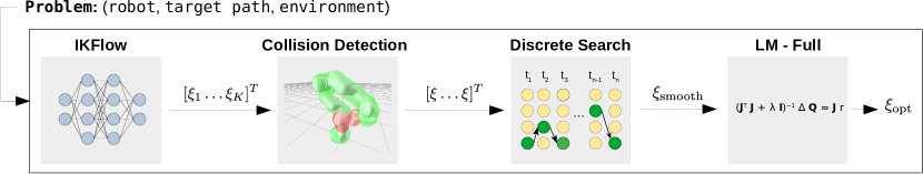
Figure 2: The CppFlow system

fig]system_diagram

In this work we present CppFlow, a novel Cartesian Path Planning planner that utilizes recent advances in learned, generative IK to generate smooth, collision free paths faster than existing SOTA methods while also succeeding on more difficult problems. Using a generative IK model addresses a key issue with trajectory optimization methods - that they work well but require a good initial solution. In this work we use the Levenberg-Marquardt algorithm for trajectory optimization, a powerful quasi-Newton optimization procedure that quickly converges to precise and constraint satisfying solutions. Additionally, a search module finds the optimally smooth config-space path by interweaving the trajectories returned by the generative IK model, which dramatically improves the quality of the optimization seed.

To evaluate CppFlow, we benchmark our method on 5 standard test problems present in the literature. To demonstrate our method’s capability on more difficult problems, we introduce a suite of new robots and target paths. The additional robots include the Franka Panda arm and a modified kinematic chain from the Fetch robot that includes a prismatic joint. As opposed to many of the existing tests which contain a basin of valid solutions, the newly introduced tests contain problems that require choosing between disjoint paths in configuration space to reveal the capability of a planner to avoid local minima. Three key metrics of planner performance are reported on: success rate, time to get an initial valid solution, and trajectory length over time. We find that CppFlow outperforms all other planners on two axes and performs comparably on the third.

II Problem Specification

The goal of the Cartesian Path Planning problem is to find a trajectory $\xi$ such that the robots end effector stays along a target path $\boldsymbol{Y}$ while satisfying additional constraints.

It is assumed that the robot has $\geq$7 Degrees of Freedom $d$ and is therefore a redundant manipulator. Owing to this additional freedom, there may be a potentially infinite set of IK solutions for a given end-effector pose. We denote the Forward Kinematics mapping as $\text{FK}(q):\mathbb{R}^{d}\rightarrow\text{SE}(3)$. The target path and trajectory are discretized into $n$ timesteps, such that $\xi=[q_{1},...,q_{n}]$ and $\boldsymbol{Y}=[y_{1},...,y_{n}]$, where $q_{i}\in\mathbb{R}^{d}$ is the robots joint configuration at timestep $i$ and $y_{i}\in\text{SE}(3)$ is the target pose at timestep $i$.

There are two paradigms to addressing time in the Cartesian Path Planning problem. Either a time parameterization is provided with the target path and the goal is to find a satisfying path that minimizes jerk or some other smoothness measure, or no time parameterization is provided, and it is assumed one is found after the joint configurations are calculated by some external module. This system uses the latter paradigm - it is assumed that an external module will calculate the temporal component of each $q_{i}$ such that the robots velocity, acceleration, and jerk limits are respected while execution time is minimized. As such, time parameterization is such omitted from this work. Given this setup, the constraints on the problem are as follows:

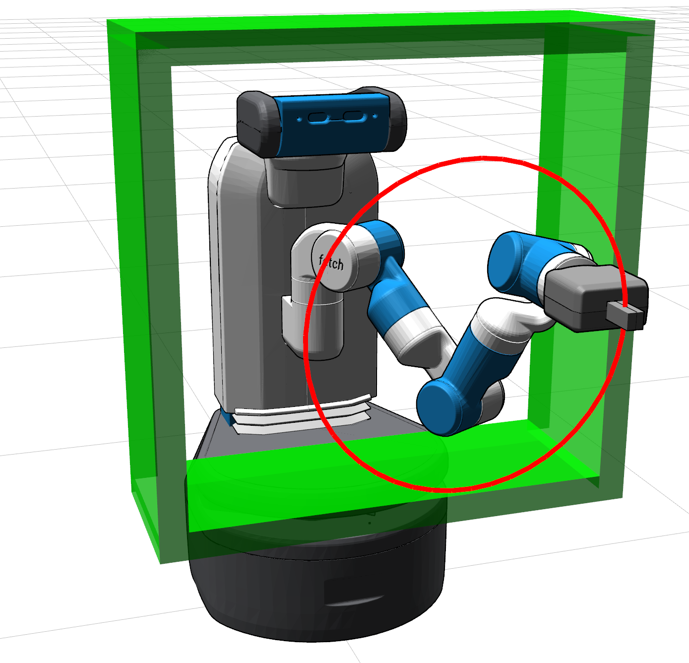
(a) Fetch.Full - Circle

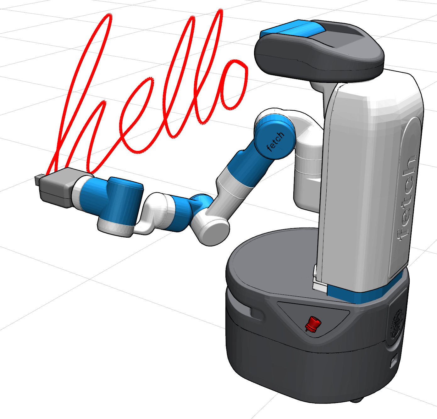
(b) Fetch.Full - Hello

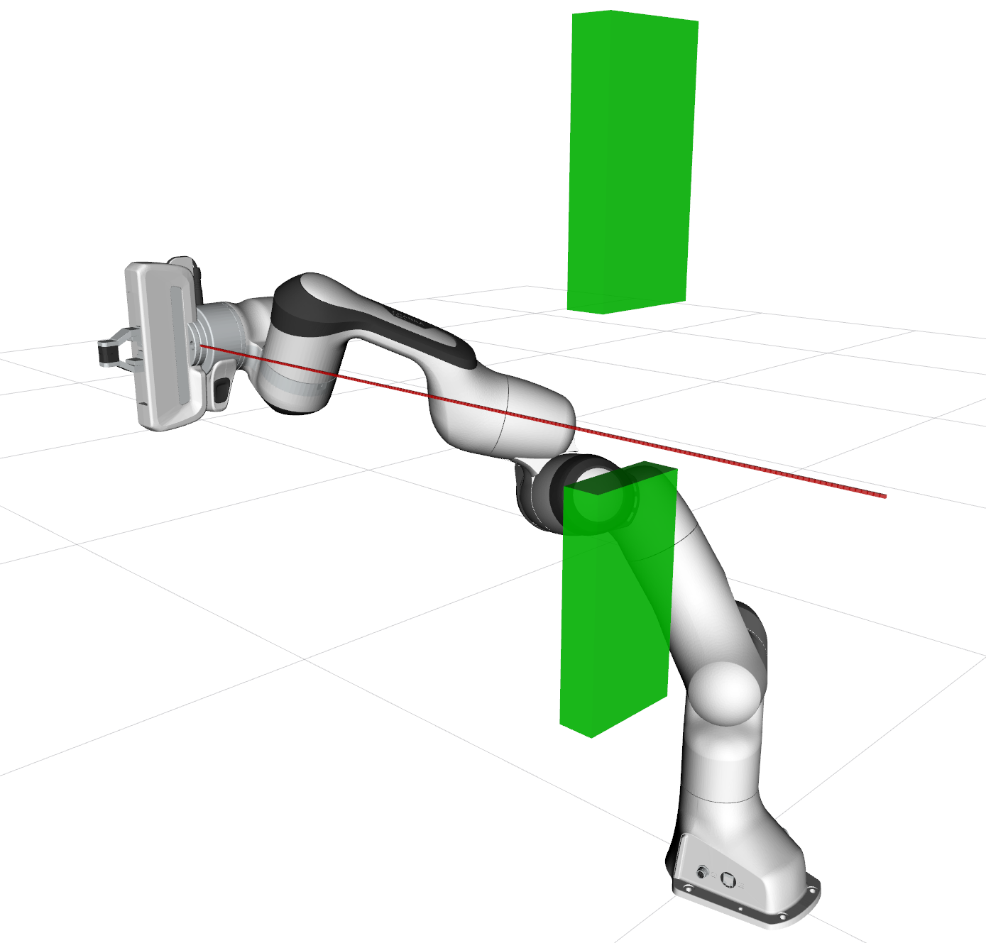
(c) Panda - flappy-bird

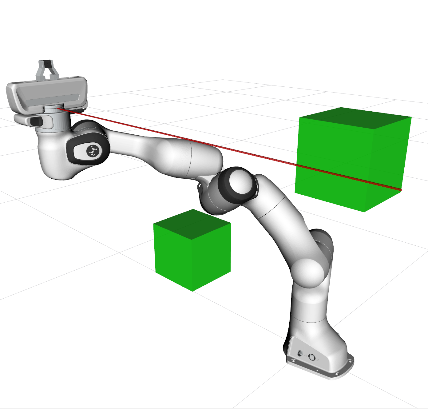
(d) Panda - 2cubes

Figure 3: Visualizations of a subset of the problems evaluated on.

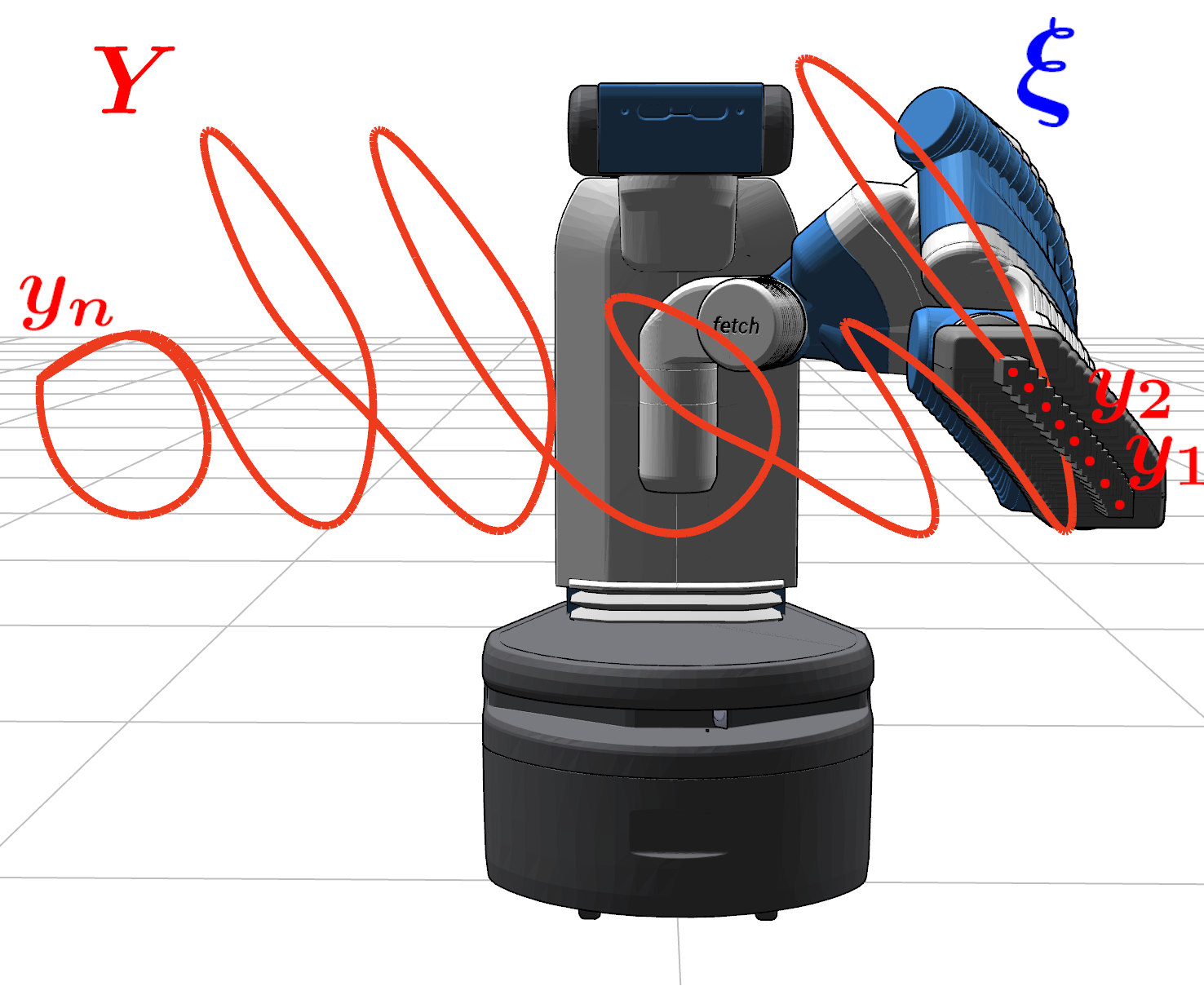
Figure 4: The ‘Fetch.Arm - hello’ problem visualized. The sweeping motion of the robots arm is generated by overlaying the first 20 configurations from a trajectory $\xi$ returned by CppFlow. The red cursive ‘hello’ is the target path, denoted $\boldsymbol{Y}$. The target path $\boldsymbol{Y}$ is composed of $n$ target poses $y_{1},...,y_{n}$

Pose error. At every timestep $i$, the deviation of the positional and rotational components of the robots end effector from the target pose, found by calculating $\text{FK}(q_{i})-y_{i}$, must be within the mechanical repeatability of the robot. Here and in the rest of the paper, the subtraction between poses in $\textrm{SE}(3)$ indicates elementwise subtraction between the x, y, z, and roll, pitch, and yaw components of each pose. Specifically, positional error is the euclidean norm of the positional difference, and rotational error is the geodesic distance between the rotational components of $\text{FK}(q_{i})$ and $y_{i}$. It is the authors view that refining a joint configuration that results in end effector displacement less then the mechanical repeatability of the robot is wasted computation, as displacements below the repeatability limit will have no impact on real hardware. Thus, a positional error threshold of 0.1 mm is assigned, as this is the reported positional mechanical repeatability of both the Franka Panda and the Fetch Manipulator. The rotational error threshold is set to 0.1 deg, which is found through a procedure that finds the expected maximum rotational error for a configuration within the region of positional repeatability.

Collision avoidance. At no timestep in the trajectory can the robot collide with itself or the environment. A virtual capsule is affixed to each link of the given robot a priori. Each capsule is the minimum enclosing capsule for a given links visual mesh and is found through a Quadratic Programming optimization procedure. Given capsules for each link, self collision checking is performed by evaluating whether any two capsules are intersecting. Checks between certain links are removed when it is impossible for these links to collide if joint limits are respected. The exact position and shape of every obstacle in the environment is assumed to be provided. In a similar manner, robot-environment collisions are found by checking for intersections between any link’s capsule and the obstacles in the environment. Obstacles are all cuboids in this work for simplicity. It is assumed that the time parameterization between configurations is small enough such that collision checks between timesteps are not required.

Joint limits. The configuration $q$ at each timestep $i$ must be within the robots joint limits.

Discontinuities. The configurations across two different timesteps must stay close to one another as large changes in configuration space may not be achievable by the robot. A value of 7 degrees and 2 cm is chosen as the maximum absolute distance an individual revolute or prismatic joint may change across a timestep, respectively.

Lastly, while not a constraint, trajectory length is an important metric for evaluating the quality of a trajectory. Trajectory length is defined as the cumulative change in configuration-space across a trajectory (measured in radians and meters) and gives an estimate for how long the trajectory will take to execute on an actual robot. The time to find a valid solution is an important metric as well. As the name suggests this is the total elapsed time before a constraint satisfying trajectory is found.

Figure 5: Trajectory length (rad) convergence results for CppFlow and Torm. Stampede results are ommited as the planner is not anytime - it returns only a single trajectory. A lower value is better, as this indicates a trajectory that can be executed in a shorter time. Plots are generated by averaging the trajectory length convergence curves of the designated planner from 10 planning runs. The mean time to a valid solution time is the first time instant plotted. The convergence behavior for CppFlow is strictly better for ‘Fetch.Full - square’ and ‘Panda - 1cube’, as measured by initial valid solution time and asymptotic limit. CppFlow has a 1.169x larger final trajectory length for ‘Fetch.Arm - circle’ problem as compared to Torm, however, it takes Torm 1.83x as long for Torm to find an initial valid trajectory for this problem.

III CppFlow

We now present the CppFlow method. It is composed of three main components: a candidate motion plan generator, a global discrete search procedure, and a trajectory optimizer.

III-A Candidate Motion Plan Generation

CppFlow begins by generating $K$ approximate motion plans using IKFlow, a learned generative IK solver ($K$ is a hyperparameter set here to 175) [6]. IKFlow generates IK solutions as a function of a latent vector $z$ and a target cartesian pose $y$, in batch on the GPU. Additionally, IKFlow models exhibit a desirable property: small changes to either the latent vector or target pose result in small changes to returned IK solutions. We use IKFlow as the generative-IK model because of this smoothness property and its low inference time and high accuracy.

To generate the $K$ motion plans, $K$ latent vectors are drawn uniformly at random from a unit hypercube, and repeated $n$ times. Randomizing the latent vectors ensures a diverse set of IK solutions, and resulting motion plans are returned. Each set of $n$ repeated latent codes is paired with a copy of the target path $\boldsymbol{Y}$. A batch of inputs is formed for IKFlow by concatenating each latent vector-target path pair to create a batch of $nK$ latent vector-target pose pairs. This batch is passed to IKFlow, which transforms it into $nK$ IK solutions. Candidate motion plans are generated by segmenting these solutions according to their original latent vector. Advantageously, the returned IK solutions for each of the $K$ approximate motion plans are found to change slowly. This is because the latent vector is held fixed and the target path is slowly changing, satisfying the conditions for the smoothness property stated above. The runtime of this procedure scales linearly with the hyperparameter $K$, target path length $n$, and as a function of the performance characteristics of the GPU.

Problem	Planner	Time to valid solution (s)	Initial solution time (s)	Planning success rate (%) - 2.5s max	Trajectory length (rad/m) - 2.5s max	Planning success rate (%) - 50s max	Trajectory length (rad/m) - 50s max
Fetch.Arm - circle	cppflow - ours	1.211	0.014	90.0	17.39	100.0	14.98
	$\textrm{stampede}^{*}$	91.566	91.566	0.0	—	100.0	11.105
	torm	2.916	0.715	50.0	14.82	100.0	12.81
Fetch.Arm - hello	cppflow - ours	1.126	0.016	100.0	64.46	100.0	62.52
	$\textrm{stampede}^{*}$	$\inf$	$\inf$	0.0	—	0.0	—
	torm	3.598	1.414	30.0	62.426	100.0	58.653
Fetch.Arm - rotation	cppflow - ours	0.535	0.014	100.0	30.423	100.0	26.758
	$\textrm{stampede}^{*}$	$\inf$	$\inf$	0.0	—	0.0	—
	torm	1.27	1.066	70.0	30.5	100.0	27.13
Fetch.Arm - s	cppflow - ours	0.788	0.014	100.0	17.18	100.0	15.47
	$\textrm{stampede}^{*}$	137.569	137.569	0.0	—	100.0	10.856
	torm	1.024	0.844	80.0	13.549	100.0	12.77
Fetch.Arm - square	cppflow - ours	0.747	0.014	100.0	21.71	100.0	18.48
	$\textrm{stampede}^{*}$	110.774	110.774	0.0	—	100.0	14.841
	torm	1.045	0.79	100.0	17.287	100.0	16.56
Fetch.Full - circle	cppflow - ours	1.02	0.011	100.0	20.13 / 0.37	100.0	13.28 / 0.46
	torm	14.595	2.363	10.0	21.99 / 0.46	90.0	20.67 / 0.45
Fetch.Full - hello	cppflow - ours	1.243	0.011	70.0	49.74 / 2.9	100.0	39.97 / 3.49
	torm	$\inf$	4.12	0.0	—	20.0	76.07 / 2.39
Fetch.Full - rotation	cppflow - ours	0.605	0.011	100.0	28.47 / 1.01	100.0	21.8 / 1.24
	torm	15.31	1.784	0.0	—	100.0	29.15 / 0.77
Fetch.Full - s	cppflow - ours	0.785	0.011	100.0	22.08 / 0.55	100.0	14.14 / 0.77
	torm	$\inf$	$\inf$	0.0	—	0.0	—
Fetch.Full - square	cppflow - ours	0.751	0.011	100.0	19.65 / 0.35	100.0	13.97 / 0.39
	torm	9.255	2.997	0.0	—	70.0	18.9 / 0.6
Panda - 1cube	cppflow - ours	0.434	0.011	100.0	8.075	100.0	7.585
	torm	2.912	2.585	0.0	—	100.0	8.13
Panda - 2cubes	cppflow - ours	0.484	0.011	100.0	9.627	100.0	9.031
	torm	62.478	39.346	0.0	—	40.0	13.21
Panda - flappy-bird	cppflow - ours	0.63	0.011	100.0	20.323	100.0	20.323
	torm	$\inf$	$\inf$	0.0	—	0.0	—

TABLE I: Results from CppFlow, Torm, and Stampede on the 13 test problems. ‘Time to Valid Solution’ - median time to find a trajectory with less than 1mm/.1deg pose error and all other constraints satisfied. ‘Initial Solution Time’ - median time to find a trajectory, regardless of its validity. Failed runs count for $\inf$ planning time for both ‘Time to Valid Solution’ and ‘Initial Solution Time’. ‘Planning Success Rate, x seconds’ - the percentage of runs which have found a valid trajectory before x seconds have elapsed. ‘Trajectory length (rad/m), x seconds’: The mean cumulative change in configuration-space of the revolute, prismatic joints of the latest valid trajectory found before x seconds have elapsed. A lower trajectory is better, as generally this means the robot can execute the trajectory faster. The astricks on the $\textrm{stampede}^{*}$ rows indicates that the planning success rate and trajectory length is for the final returned trajectory, which may be returned after 50s. Stampede failed to run at all with the Fetch.Full kinematic chain so was excluded from the results. CppFlow returns an initial solution faster than either of the other methods on all problems. It will take Torm and Stampede 19.84x and 132.8x as long on average respectively to find a valid solution.

III-B Global discrete search

The objective of the global discrete search module is to find the optimal $\xi$ as measured by collision avoidance and the Maximum Joint Angle Change (mjac) - the maximum absolute change in joint angle between any two timesteps along a trajectory. Formally, $\texttt{mjac}=\max(\max(|q_{i+1}[j]-q_{i}[j]|\forall j\in[1,...,d])\forall i\in[1,...,n])$.

The module first creates a directed graph from the $K$ motion plans. Each IK solution is considered a node. Edges are connected from each IK solution to the $K$ IK solutions at the following time step. A dynamic-programming-based search procedure is run on the graph. The cost at each node is set to the minimum mjac achievable if the node is included in the returned path. To avoid trajectories that are close to the joint limits, an additional cost of 10 (which is greater than the possible mjac cost of $\pi$ for revolute joints, and the range of the prismatic joint for Fetch.Full) is added to configurations that are within 1.5 degrees/3 cm of their joint limits. An additional cost of 100 is added to configurations that would lead to a collision. Upon completion, a backtracking procedure is executed, which returns $\xi_{\textrm{search}}$.

Trajectories with large mjac values are likely to fail in the next step, as this indicates the existence of large joint space discontinuities, which are difficult to optimize. To remedy this, after the search finishes, the mjac of $\xi_{\textrm{search}}$ is calculated. If it is above a threshold (12 deg/3 cm), an additional set of motion plans is generated and added to the existing set before repeating the search. Collision and joint limit checks performed on the initial plans are retained to conserve computation. This is an effective approach to prevent bad optimization seeds, based on the intuition that a denser covering of the relevant portions of configuration space likely contains a better configuration space path.

III-C Levenberg-Marquardt for Trajectory Optimization

The optimization problem is framed as a nonlinear least squares problem and solved using the Levenberg-Marquardt algorithm. As opposed to stochastic gradient descent and other first-order optimization methods previously used to solve this problem [5], Levenberg-Marquardt approximates the objective Hessian matrix with first derivative information in order to make significantly larger and more accurate steps on least-squares objectives. As a result, when initial seeds are in close vicinity to a valid solution, only 1 to 3 steps are required to find a valid solution.

The optimizer keeps track of the latest valid solution; this can be returned if the user wants to exit making CppFlow an anytime planner i.e., it continuously improves its plan until stopped. If a valid solution is not found, the dynamic programming search is repeated using additional motion plans from IKFlow. This lowers the mjac of the $\xi$ used as a seed, increasing the chance it will be successfully optimized.

Similar to Torm, a non-stationary objective function is used, leading to improved convergence performance [5]. The optimizer switches between optimizing only for pose error and for trajectory length and obstacle avoidance. To balance the frequency of the two, the optimizer optimizes for pose error exclusively until the positional and rotational error of the end effector is below the respective specified threshold at every timestep. A trajectory length and obstacle avoidance optimization step is then taken, after which the optimizer switches back to pose only, and the cycle continues. This ordering ensures that the trajectory stays close to a valid solution throughout the optimization process. The residual terms are $r_{\textrm{pose}}$ for pose error, and $r_{\textrm{diff}}$ for trajectory length and obstacle avoidance error. Figure 6 shows the composition of each residual. The residual components are listed below.

$$r_{\textrm{pose}}=\begin{bmatrix}\textrm{FK}(q_{1}).x-y_{1}.x\\ \textrm{FK}(q_{1}).y-y_{1}.y\\ \textrm{FK}(q_{1}).z-y_{1}.z\\ \textrm{FK}(q_{1}).\Phi-y_{1}.\Phi\\ \textrm{FK}(q_{1}).\Theta-y_{1}.\Theta\\ \textrm{FK}(q_{1}).\Psi-y_{1}.\Psi\\ \dots\\ \textrm{FK}(q_{n}).\Psi-y_{n}.\Psi\\ \end{bmatrix}$$

$$r_{\textrm{diff}}=\begin{bmatrix}q_{2}-q_{1}\\ q_{3}-q_{2}\\ \dots\\ q_{n}-q_{n-1}\\ \textrm{self-coll-dist}(q_{1})\\ \dots\\ \textrm{self-coll-dist}(q_{n})\\ \textrm{env-coll-dist}(q_{1})\\ \dots\\ \textrm{env-coll-dist}(q_{n})\\ \end{bmatrix}$$

Figure 6: The residual term used by the optimizer. The symbols $\Phi$, $\Theta$, and $\Psi$ represent the roll, pitch, and yaw of the pose.

Pose error The pose of the end effector at each timestep is calculated by a Forward Kinematics function using an efficient custom PyTorch implementation which performs calculations in parallel on the GPU. A residual term for the error in the x, y, z, and roll, pitch, and yaw dimensions ($\textrm{FK}(q_{i}).x-y_{i}.x$, …, $\textrm{FK}(q_{i}).\Psi-y_{i}.\Psi$) are added to $r_{\textrm{pose}}$, for every $q_{i}$ in $\xi$. The Jacobian of these residuals wrt $\xi$ is found by observing that in the derivative of $\textrm{FK}(q_{i}).x-y_{i}.x$ wrt $q_{i}$, the constant term $y_{i}.x$ goes to 0 so the derivative is $J_{\textrm{fk}}(q_{i}).x$. A second custom PyTorch implementation quickly calculates this kinematic Jacobian term in parallel on the GPU. Once the residual and Jacobian are calculated, the Levenberg-Marquardt update $(J^{T}J+\lambda I)\Delta\xi=Jr_{\textrm{pose}}$ is calculated using PyTorch’s batched LU decomposition functionality.

Trajectory length. A differencing loss is used as a surrogate error for trajectory length. It penalizes changes in joint angle across consecutive timesteps: $q_{i+1}-q_{i}\forall i\in[1,...,n-1]$, which encourages configurations to stay close to one another. The Jacobian of each differencing error $(q_{i+1}-q_{i})$ wrt $\xi$ is the identity matrix for configuration $q_{i+1}$, and the negated identity matrix for $q_{i}$.

Robot-robot collision avoidance. For self-collision checking, each robot is represented as a set of capsules with endpoints $(a,b)$ and radius $c$. As in [7], we formulate the minimum distance between a capsule pair $(a_{1},b_{1},c_{1})$ and $(a_{2},b_{2},c_{2})$ as the minimum cost, less $c_{1}+c_{2}$, of a convex quadratic program

$$\min_{t_{1},t_{2}}\quad (a_{1}+(b_{1}-a_{1})t_{1})^{T}(a_{2}+(b_{2}-a_{2})t_{2})$$

subject to $$0\leq t_{1},t_{2}\leq 1$$

which we solve with a custom batched active-set method implementation. While the solutions of convex programs are differentiable [8], since we evaluate many collision pairs for the same joint configuration, it is efficient to compute Jacobians by batched forward-mode [9] automatic differentiation.

Joint limits. During optimization, joint limit constraints are enforced by clamping $\xi$ to the robot joint limits.

Robot-environment collision avoidance. We represent obstacles as cuboids with arbitrary spatial positioning. We formulate the minimum distance between a capsule and a cuboid in a frame axis-aligned to the cuboid, in which the capsule has endpoints $(a,b)$ and radius $r$, and the cuboid has extents $p_{min}=(x_{min},y_{min},z_{min})$ and $p_{max}=(x_{max},y_{max},z_{max})$ as the minimum cost, less $c$, of the convex quadratic program.

$$\min_{t,p}\quad p^{T}(a+(b-a)t)$$

subject to $$0\leq t\leq 1$$

$$p_{min}\leq p\leq p_{max}$$

IV Experiments & Analysis

CppFlow is evaluated on 13 different planning problems and 3 different robots. Other SOTA methods, including Torm and Stampede [5, 3] are also evaluated to provide a comparison. The Fetch.Arm problems are the same as reported in  [5]. The Fetch.Full problems are the same except for the addition of the Fetch prismatic joint to the kinematic chain. The Panda problems were created in this work.

We grade the planner on three axes: success rate, time to get an initial valid solution, and trajectory length over time. Metrics include the time to find a valid solution (maximum of .1 mm position and .1 degree rotation error without violating any other constraints), initial solution time (regardless of validity), planning success rate, and trajectory length. For CppFlow and Torm, which are anytime, these are reported throughout the optimization whereas for Stampede only the final returned trajectory is analyzed.

IV-A Experiments

There are four obstacle-free problems, including ‘hello’, ‘rotation’ for both Fetch.Full and Fetch.Arm. The problems with obstacles include ‘circle’, ‘s’, and ‘square‘ for Fetch.Full and Fetch.Arm and the three Panda problems. These are visualized in 3. While Torm allows for an initial joint configuration to be set, this feature is disabled for a fair comparison. Further, the target path for the ‘rotation’ problems provided in the Torm GitHub repository had 40 additional waypoints added to reduce the distance between the poses of the target path. The poses still parameterize the same motion, however. We run Stampede on the obstacle problems even though it does not account for obstacles as a further point of comparison - the obstacles are ignored in these cases. A software bug in the provided code prevented Stampede from running on the Fetch.Full robot.

The three test robots are ‘FetchArm’, ‘FetchFull’, and ‘Panda’ (7, 8, and 7 DOF, respectively). The difference between ‘FetchArm’ and ‘FetchFull’ is that ‘FetchFull’ includes a prismatic joint (the ‘torso_lift_joint’) which lifts the entire arm. Each planner is run 10X on each problem. CppFlow and Torm are allotted 60s per run, whereas Stampede has no time limit (it stops on its own after returning a solution). Tests are run on an Intel i9 with 20 CPUs, 124 GBs of RAM, and an Nvidia RTX 4090 graphics card.

IV-B Results

The numerical results are presented in Table I; selected trajectory length convergence plots are shown in Figure 5.

CppFlow dominates on the first axis, planning success rate. The success rate is 100% for all problems after 50s and reaches 96.7% on average after only 2.5 seconds. In comparison, Torm fails to generate any plans more than 50% of the time on three of the problems, and Stampede fails to generate any plans for 2/5 of its problems. This indicates CppFlow is a robust planner that is likely to succeed on difficult problems. CppFlow also dominates on the second axis: the time to get a valid solution. Valid solutions are generally found within 1 second and often in under 600ms. Compared to CppFlow, Torm takes between 1.29x to 129.15x as long to find its first valid solution. On average, it will take Torm 19.84x as long to find a valid solution. On the final axis, the trajectory length convergence behavior for CppFlow is strictly better for the Fetch.Full and Panda problems compared to Torm. The convergence results are roughly tied for 2/5 Fetch.Arm problems, while Torm has a lower asymptotic limit for the other 3 (including ‘Fetch.Arm - circle’, which is shown in Figure 5). The results indicate that CppFlow generates valid solutions faster than all other SOTA methods while producing trajectories of overall similar quality when run as an anytime planner. Crucially, CppFlow succeeds on the hardest problems, which indicates it is a highly capable planner. Given this, CppFlow would be a good all-around choice for a CPP planner, especially in settings that require quick planning times for unseen and potentially difficult planning problems, such as in a home or hospital.

V Related work

Torm solves CPP using gradient descent-based optimization to reach an acceptable solution [5]. It contains a candidate trajectory generator module that performs traditional IK along the reference trajectory to find a good approximate trajectory to optimize. RelaxedIK solves the problem of generating motion in real-time, which satisfies end-effector pose goal matching and motion feasibility [1]. Stampede [3] solves time-constrained CPP by constructing and searching through a solution graph of viable configurations to find a satisfying trajectory. Luo and Hauser solve time-constrained CPP [10] through a decoupled optimization procedure in which pose error is first reduced before temporal matching is decoupled; however, only the position of the end effector is considered - orientation is ignored. While IK for redundant kinematic chains has been traditionally solved by using the Jacobian to iteratively optimize joint configuration, recent work has shown that generative modeling techniques can learn this mapping instead. These methods generate solutions in parallel on the GPU, enabling significantly better runtime scaling characteristics, albeit at the cost of accuracy. IKFlow [6], the solver used here, uses conditional Normalizing Flows to represent this mapping. The method in [11] learns the density of IK solutions at a given pose using a Block Neural Autoregressive Flow. NodeIK learns this mapping using a Neural Ordinary Difference Equation model [12]. In [13] Generative Adversarial Networks for IK are trained for the Fetch Manipulator and used for generating trajectories along a path; however, statistics on the pose error of returned solutions are not included. In [14], the IK problem is reformulated as a distance geometry problem whose solutions are learned via Graph Neural Networks. A single GNN can produce IK solutions for multiple kinematic chains. However, the resulting solution accuracy for individual robots is lower than that of IKFlow and NodeIK.

VI Conclusion

We propose an efficient and capable anytime Cartesian Path Planner that combines techniques from search, optimization and learning to achieve SOTA results. Our planner achieves a 100% success rate on a representative problem set and finds valid trajectories within 1.3 seconds, in the worst case. Additionally, it continually decreases trajectory length when time is allowed. Our results demonstrate the usefulness of generative IK models for kinematic planning and raise the question of where else they can be applied. We are exploring how CppFlow may be adapted for kinodynamic planning, which requires precise temporal specifications.

References

- [1] D. Rakita, B. Mutlu, and M. Gleicher, “RelaxedIK: Real-time synthesis of accurate and feasible robot arm motion,” in Robotics: Science and Systems XIV. Robotics: Science and Systems Foundation, 2018. [Online]. Available: http://www.roboticsproceedings.org/rss14/p43.pdf
- [2] M. Kang, Y. Cho, and S.-E. Yoon, “RCIK: Real-time collision-free inverse kinematics using a collision-cost prediction network,” vol. 7, no. 1, pp. 610–617, conference Name: IEEE Robotics and Automation Letters.
- [3] D. Rakita, B. Mutlu, and M. Gleicher, “STAMPEDE: A discrete-optimization method for solving pathwise-inverse kinematics,” in 2019 International Conference on Robotics and Automation (ICRA), 2019, pp. 3507–3513, ISSN: 2577-087X.
- [4] R. M. Holladay and S. S. Srinivasa, “Distance metrics and algorithms for task space path optimization,” in 2016 IEEE/RSJ International Conference on Intelligent Robots and Systems (IROS), 2016, pp. 5533–5540.
- [5] M. Kang, H. Shin, D. Kim, and S.-E. Yoon, “TORM: Fast and accurate trajectory optimization of redundant manipulator given an end-effector path,” 2020. [Online]. Available: http://arxiv.org/abs/1909.12517
- [6] B. Ames, J. Morgan, and G. Konidaris, “Ikflow: Generating diverse inverse kinematics solutions,” 2022.
- [7] M. Safeea, P. Neto, and R. Bearee, “Efficient calculation of minimum distance between capsules and its use in robotics,” IEEE Access, vol. 7, pp. 5368–5373, 2018.
- [8] B. Amos and J. Z. Kolter, “Optnet: Differentiable optimization as a layer in neural networks,” in International Conference on Machine Learning. PMLR, 2017, pp. 136–145.
- [9] J. M. Siskind and B. A. Pearlmutter, “Perturbation confusion and referential transparency,” 2005.
- [10] J. Luo and K. Hauser, “Interactive generation of dynamically feasible robot trajectories from sketches using temporal mimicking,” in 2012 IEEE International Conference on Robotics and Automation, 2012, pp. 3665–3670.
- [11] S. Kim and J. Perez, “Learning reachable manifold and inverse mapping for a redundant robot manipulator,” in 2021 IEEE International Conference on Robotics and Automation (ICRA), 2021, pp. 4731–4737.
- [12] S. Park, M. Schwartz, and J. Park, “NODE IK: Solving inverse kinematics with neural ordinary differential equations for path planning.” [Online]. Available: http://arxiv.org/abs/2209.00498
- [13] H. Ren and P. Ben-Tzvi, “Learning inverse kinematics and dynamics of a robotic manipulator using generative adversarial networks,” Robotics Auton. Syst., vol. 124, p. 103386, 2020.
- [14] O. Limoyo, F. Marić, M. Giamou, P. Alexson, I. Petrović, and J. Kelly, “One network, many robots: Generative graphical inverse kinematics,” 2022.