Wasserstein Contraction of Geodesic Slice Sampling on the Sphere A Dimension-Independent Bound on the Wasserstein Contraction Rate of Geodesic Slice Sampling on the Sphere for Uniform Target Philip Schär, Thilo D. Stier MCMC; slice sampling; Wasserstein contraction; geodesic random walk 60J05; 60G50; 65C05 September 16, 2023 (…) 0 2020 0 10.1214/YY-TN When faced with a constant target density, geodesic slice sampling on the sphere simplifies to a geodesic random walk. We prove that this random walk is Wasserstein contractive and that its contraction rate stabilizes with increasing dimension instead of deteriorating arbitrarily far. This demonstrates that the performance of geodesic slice sampling on the sphere can be entirely robust against dimension-increases, which had not been known before. Our result is also of interest due to its implications regarding the potential for dimension-independent performance by Gibbsian polar slice sampling, which is an MCMC method on $\R^{d}$ that implicitly uses geodesic slice sampling on the sphere within its transition mechanism.

1 Introduction

Geodesic slice sampling on the sphere (GSSS) [2] is a Markov chain Monte Carlo (MCMC) method for approximate sampling from (typically intractable) distributions on the $(d-1)$-sphere

$$\mathbb{S}^{d-1}:=\{x\in\R^{d}\mid\norm{x}=1\}$$

(where $\norm{\cdot}$ denotes the Euclidean norm). More specifically, GSSS assumes a target distribution $\nu$ on $(\mathbb{S}^{d-1},\mathcal{B}(\mathbb{S}^{d-1}))$ (the sphere equipped with its Borel $\sigma$-algebra) to be given by a potentially unnormalized density, i.e. a measurable function $\varrho:\mathbb{S}^{d-1}\rightarrow\,[0,\infty[$ such that

$$\nu(A)=\frac{\int_{A}\varrho(x)\sigma_{d-1}(\text{d}x)}{\int_{\mathbb{S}^{d-1}}\varrho(x)\sigma_{d-1}(\text{d}x)},\qquad A\in\mathcal{B}(\mathbb{S}^{d-1}),$$

where $\sigma_{d-1}$ denotes the surface measure on $(\mathbb{S}^{d-1},\mathcal{B}(\mathbb{S}^{d-1}))$. In [2], the authors propose two different variants of the method, ideal geodesic slice sampling and geodesic shrinkage slice sampling. Both perform an iteration from an old state $X_{n-1}=x_{n-1}$ to a new state $X_{n}=x_{n}$ by the following three steps:

1. Draw a threshold $T_{n}\sim\mathcal{U}(\!\,]0,\varrho(x_{n-1})[)$, call the result $t_{n}$.

2. Choose a geodesic $g_{n}:\,[0,2\pi[\rightarrow\mathbb{S}^{d-1}$ that runs through $x_{n-1}$, uniformly at random among all such geodesics.

3. Draw the new state $X_{n}$ from a distribution supported only on the intersection

   $$L(t_{n},g_{n}):=L(t_{n})\cap g_{n}(\!\,[0,2\pi[)$$

   of the image of $g_{n}$ with the super-level set (or slice) of $\varrho$ w.r.t. $t_{n}$,

   $$L(t_{n}):=\{x\in\mathbb{S}^{d-1}\mid\varrho(x)>t_{n}\}.$$

The difference between the two variants of GSSS lies in the distribution they use for the third step. Ideal geodesic slice sampling simply uses the uniform distribution, i.e. it samples $X_{n}\sim\mathcal{U}(L(t_{n},g_{n}))$. Motivated by the infeasibility (in many cases) of efficiently implementing the sampling from this uniform distribution, geodesic shrinkage slice sampling instead employs a shrinkage procedure (a sort of adaptive acceptance/rejection method), which approximates sampling from the same distribution (and coincides with it under certain conditions) while being straightforward to implement efficiently. We refer to [2] for more details.

It is shown in [2, Lemmas 14, 24] that both variants of GSSS are well-defined and reversible w.r.t. the target distribution $\nu$, under the weak assumption (only required for geodesic shrinkage slice sampling) that $\varrho$ is lower semi-continuous. Moreover, in [2, Theorems 15, 26] the authors prove, under somewhat stronger assumptions on $\varrho$, that both variants of GSSS are uniformly geometrically ergodic (i.e. their iterate distribution converges geometrically to their target distribution in terms of the total variation distance, with the guaranteed convergence speed not depending on where they are initialized).

In this paper, we examine the Wasserstein contraction rate of GSSS for the specific case that $\varrho$ is constant, so that $\nu=\mathcal{U}(\mathbb{S}^{d-1})$. Although this distribution is actually tractable, our motivation for examining this setting is twofold:

• On the one hand, it is known that Wasserstein contraction is robust against perturbations of the transition kernel (which may result from perturbations of the target distribution) that are small in a suitable sense. Therefore, by showing that GSSS is Wasserstein contractive for a constant target density, we also obtain this property (albeit with a worse contraction rate) for target densities that are close to constant. We refer to [6, Remark 54] for details.

• On the other hand, the performance of GSSS for a constant target density is intimately related to the question of dimension-independence of Gibbsian polar slice sampling (GPSS) [11], which is an MCMC method on $\R^{d}$ that implicitly uses GSSS within its transition mechanism.

We elaborate on the second point. GPSS is constructed to approximate polar slice sampling (PSS) [7], an abstract MCMC method on $\R^{d}$ that has some very remarkable theoretical properties but is infeasible to implement efficiently in all but a few toy settings. For PSS, it was shown in [8, 10] that it performs dimension-independently well for both a class of light-tailed (more specifically log-concave) [8] and a class of heavy-tailed target densities [10]. In constructing GPSS, the authors hoped to retain this dimension-independence of PSS also for its approximation GPSS. However, theoretical results in this regard are, as yet, unavailable. Moreover, as mentioned before, GPSS internally uses GSSS for its transitions, which strongly suggests that the theoretical properties of GSSS must also play a role for those of GPSS.

The settings in which PSS is known to perform dimension-independently well have the commonality that the target density is always assumed to be rotationally invariant around the coordinate origin. GPSS for these settings only uses GSSS in the particular case of the target density being constant. The aforementioned uniform geometric ergodicity results [2, Theorems 15, 26] for GSSS apply to this case, but their key quantity, the convergence rate $\rho<1$ slowly tends to $1$ as $d\rightarrow\infty$. In other words, the only available quantitative theoretical result regarding GSSS for a constant target density does not guarantee a dimension-independent performance. This suggests that the present theoretical understanding of GSSS is insufficient for proving that GPSS performs dimension-independently well under the same conditions as PSS (which numerical experiments on GPSS suggest to be the case).

However, a simple numerical experiment on GSSS suggests that the uniform geometric ergodicity result is overly pessimistic for constant targets, in that the actual dimension-dependence of the performance of GSSS in this setting appears to be negligible, at least when measured in terms of the mean integrated autocorrelation time (IAT), see Figure 1. With our main result, we demonstrate that this impression is correct. That is, we prove dimension-independent performance guarantees for GSSS with a constant target, specifically showing that its Wasserstein contraction rate is upper-bounded by $0.86$ in all dimensions $d\geq 3$.

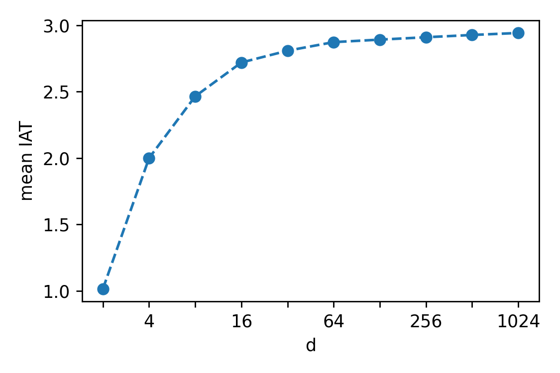
Figure 1: Empirical dimension-dependence of GSSS for uniform target, measured by the mean IAT of its samples. In each of the dimensions $d=2^{1},\dots,2^{10}$, we ran the sampler $n_{\text{rep}}=10$ times for $n_{\text{its}}=10^{4}$ iterations per run, computed the mean IAT of the $n_{\text{its}}$ samples in each run and averaged these values over the $n_{\text{rep}}$ repetitions to minimize noise. The plot shows that the mean IAT initially worsens with increasing dimension, but then plateaus around a constant value near $3$. This suggests that the sampler’s performance stabilizes with increasing dimension instead of deteriorating arbitrarily far.

The remainder of this paper is structured as follows. In Section 2, we provide some background on the geodesics of $\mathbb{S}^{d-1}$ and a formal description of the random walk we are analyzing, note connections to some related work, and then give some more background on the concept of Wasserstein contraction. Afterwards, in Section 3, we state and prove our main result. We conclude with a detailed discussion of that result in Section 4.

2 Preliminaries

We begin by providing a formal description of GSSS for a constant target. Arbitrarily fix $x\in\mathbb{S}^{d-1}$. We denote by $\mathbb{S}^{d-2}_{x}\subseteq\mathbb{S}^{d-1}$ the great subsphere w.r.t. $x$, i.e. the set

$$\mathbb{S}^{d-2}_{x}:=\{z\in\mathbb{S}^{d-1}\mid x^{T}z=0\},$$

and by $\sigma_{d-2}^{(x)}$ the natural surface measure on $\mathbb{S}^{d-2}_{x}$. Since the great subsphere w.r.t. $x$ corresponds to the unit sphere in the tangent space to $\mathbb{S}^{d-1}$ at $x$, it parametrizes the geodesics running through $x$. That is, for any $z\in\mathbb{S}^{d-2}_{x}$, a geodesic (which on $\mathbb{S}^{d-1}$ is the same as a great circle) through $x$ is given by the unit velocity curve

$$g_{x,z}:\,[0,2\pi[\rightarrow\mathbb{S}^{d-1},\;\omega\mapsto\cos(\omega)x+\sin(\omega)z.$$ (1)

We denote by $G_{x,z}:=g_{x,z}(\!\,[0,2\pi[)\subset\mathbb{S}^{d-1}$ the image of $g_{x,z}$.

By construction, drawing a reference point $z\in\mathbb{S}^{d-2}_{x}$ from the uniform distribution over $\mathbb{S}^{d-2}_{x}$ w.r.t. $\sigma_{d-2}^{(x)}$ (which we denote $\mathcal{U}(\mathbb{S}^{d-2}_{x})$) to determine a geodesic $g_{x,z}$ through $x$ amounts to a reasonable notion of a uniform distribution over all such geodesics. Moreover, due to the constant velocity of $g_{x,z}$, drawing $\Omega\sim\mathcal{U}(\!\,[0,2\pi[)$ and applying $g_{x,z}$ to the result implements a reasonable notion of a uniform distribution over $G_{x,z}$ (which we denote $\mathcal{U}(G_{x,z})$). We refer to [2, Section 2] and the references therein for more details.

We now turn our focus back to GSSS. Recall the abstract description of GSSS from Section 1. If we assume the target density $\varrho$ to be constant, the threshold $t_{n}$ generated in the first step becomes irrelevant, since for every $t_{n}$ that can occur, the resulting slice is $L(t_{n})=\mathbb{S}^{d-1}$. In such cases, the third step of both ideal geodesic slice sampling and geodesic shrinkage slice sampling draws the new state $x_{n}$ from the uniform distribution over the image of the geodesic $g_{n}$ chosen in the second step. A transition of the resulting Markov chain from an old state $X_{n-1}=x_{n-1}$ to a new state $X_{n}=x_{n}$ can therefore be implemented by the following two steps:

1. Draw $Z_{n}\sim\mathcal{U}(\mathbb{S}^{d-2}_{x_{n-1}})$, call the result $z_{n}$.

2. Draw $X_{n}\sim\mathcal{U}(G_{x_{n-1},z_{n}})$, call the result $x_{n}$.

In other words, given the old state, the chain uniformly at random chooses a geodesic through it and then uniformly at random chooses a point on that geodesic to be used as the new state. We can alternatively express this transition mechanism by a Markov kernel $P$ on $\mathbb{S}^{d-1}\times\mathcal{B}(\mathbb{S}^{d-1})$ defined by

$$P(x,A):=\frac{1}{2\pi\;\sigma_{d-2}^{(x)}(\mathbb{S}^{d-2}_{x})}\int_{\mathbb{S}^{d-2}_{x}}\int_{0}^{2\pi}\mathbb{1}_{A}(g_{x,z}(\omega))\text{d}\omega\,\sigma_{d-2}^{(x)}(\text{d}z)\\$$ (2)

for $x\in\mathbb{S}^{d-1},A\in\mathcal{B}(\mathbb{S}^{d-1})$.

The Markov chain $(X_{n})_{n\in\mathbb{N}_{0}}$ we described above constitutes what is commonly called a geodesic random walk. Although the convergence properties of some similar random walks have been investigated before, we are, to our knowledge, the first to study this particular walk in that regard. For an overview of the random walks most closely related to it, we refer to [2, Remarks 7–11].

Let us, however, emphasize some parallels between this paper and one other work: In [4], the authors consider a geodesic random walk on a large class of Riemannian manifolds, which on $\mathbb{S}^{d-1}$ boils down to uniformly at random choosing a geodesic (exactly like our walk does), then deterministically moving along it by a fixed step size (a hyperparameter) and using the resulting point as the next state of the Markov chain. Although the resulting walk is markedly different from the one we are interested in, we note that [4] analyze it using concepts very similar to those we use, relying also on a notion of contraction w.r.t. Wasserstein distances to prove rapid mixing. On the other hand, we emphasize that their proof strategy is entirely different from ours, likely because they cover a broad class of manifolds at once, whereas we make extensive use of the unique symmetry properties of $\mathbb{S}^{d-1}$.

Before we can close in on proving our main result, we need to briefly introduce the relevant notions concerning Wasserstein contraction. For two probability measures $\xi_{1},\xi_{2}$ on $(\mathbb{S}^{d-1},\mathcal{B}(\mathbb{S}^{d-1}))$, denote by $\Gamma(\xi_{1},\xi_{2})$ the set of couplings between them, i.e. of probability measures $\gamma$ on $(\mathbb{S}^{d-1}\times\mathbb{S}^{d-1},\mathcal{B}(\mathbb{S}^{d-1}\times\mathbb{S}^{d-1}))$ that satisfy

$$\gamma(A\times\mathbb{S}^{d-1})=\xi_{1}(A),$$

$$\gamma(\mathbb{S}^{d-1}\times A)=\xi_{2}(A)$$

for any $A\in\mathcal{B}(\mathbb{S}^{d-1})$. It is easy to see that the restriction of the Euclidean distance on $\R^{d}$ to $\mathbb{S}^{d-1}\subseteq\R^{d}$ constitutes a metric on $\mathbb{S}^{d-1}$. We can therefore define the Wasserstein distance between $\xi_{1}$ and $\xi_{2}$ w.r.t. the Euclidean distance,

$$\mathcal{W}(\xi_{1},\xi_{2}):=\inf_{\gamma\in\Gamma(\xi_{1},\xi_{2})}\int_{\mathbb{S}^{d-1}\times\mathbb{S}^{d-1}}\norm{v_{1}-v_{2}}\gamma(\text{d}v_{1}\times\text{d}v_{2}).$$

Let $P$ be a Markov kernel on $\mathbb{S}^{d-1}\times\mathcal{B}(\mathbb{S}^{d-1})$, then its Dobrushin coefficient (w.r.t. the Euclidean distance) is given by

$$\textsf{Dob}(P):=\sup_{x,y\in\mathbb{S}^{d-1},x\neq y}\frac{\mathcal{W}(P(x,\cdot),P(y,\cdot))}{\norm{x-y}},$$

see [1, Definition 20.3.1, Lemma 20.3.2]. One now says that $P$ is Wasserstein contractive with rate $\rho$ if $\textsf{Dob}(P)\leq\rho<1$.

Generally speaking, Wasserstein contraction is an extremely powerful property: If $P$ is Wasserstein contractive with rate $\rho$ and admits $\nu$ as its invariant distribution, then for any distribution $\xi$ on $(\mathbb{S}^{d-1},\mathcal{B}(\mathbb{S}^{d-1}))$ one has

$$\mathcal{W}(\xi P^{n},\nu)\leq\rho^{n}\mathcal{W}(\xi,\nu),\qquad n\in\mathbb{N}_{0},$$ (3)

where $\xi P^{n}$ corresponds to the distribution of $X_{n}$ when $(X_{n})_{n\in\mathbb{N}_{0}}$ is a Markov chain with initial distribution $\xi$ and transition kernel $P$. Moreover, it is well-known (see [6, Proposition 30]) that, in the same setting, one gets

$$\textsf{gap}_{\nu}(P)\geq 1-\rho,$$ (4)

where $\textsf{gap}_{\nu}(P)$ denotes the ($L_{2}$-)spectral gap of $P$. The spectral gap is known to be a key property of Markov chains, as it quantifies both the convergence speed in terms of the total variation distance and the asymptotic sample quality in terms of Monte Carlo integration errors. For details, we refer to [8, Sections 1-2] and the references therein. Simply put, an explicit estimate of the Wasserstein contraction rate (we use this term synonymously to Dobrushin coefficient) of a kernel $P$ yields not only the geometric convergence (3) but also an explicit estimate (4) of the spectral gap and the various powerful results this entails.

3 Main Result

Using the concepts presented in Section 2, we can now formulate our main result:

Theorem 3.1.

Let $d\geq 3$ and denote by $P$ the transition kernel (2) of GSSS for a constant target density $\varrho$ on $\mathbb{S}^{d-1}$. Then $P$ is Wasserstein contractive with rate

$$\rho:=\frac{1}{2\pi}\int_{0}^{2\pi}\sqrt{\cos^{2}(\omega)+\frac{\sin^{2}(\omega)}{d-1}}\;\text{d}\omega.$$ (5)

We postpone a discussion of this result to the next section and focus here on proving it. Before we delve into any computations, we observe that the inherent symmetry of $\mathbb{S}^{d-1}$ and the random walk (2) on it allow us to make some important simplifications to the definition of $\textsf{Dob}(P)$ (we fix $P$ to be as in (2) from now on) in our particular case. Namely, due to the rotational symmetry, $\mathcal{W}(P(x,\cdot),P(y,\cdot))$ for any $x,y\in\mathbb{S}^{d-1}$ can only depend on the (Euclidean) distance between $x$ and $y$, not on their absolute positions on the sphere. It is therefore sufficient to arbitrarily fix $x\in\mathbb{S}^{d-1}$ and choose $S$ to be the image of a geodesic $g_{x,z}$ through $x$ from which $x$ itself is removed, i.e. $S=G_{x,z}\setminus\{x\}$. As we may freely choose both $x$ and $z$, we choose them as points whose Euclidean coordinates are convenient to our proof, specifically

$$\begin{split}&x:=(1,0,\dots,0)^{T}\in\mathbb{S}^{d-1},\\ &z:=(0,1,0,\dots,0)^{T}\in\mathbb{S}^{d-2}_{x}.\end{split}$$ (6)

Note that this choice of $z$ yields

$$S:=G_{x,z}\setminus\{x\}=\{y_{\alpha}:=(\cos(\alpha),\sin(\alpha),0,\dots,0)^{T}\in\mathbb{S}^{d-1}\mid\alpha\in\,]0,2\pi[\,\}.$$ (7)

Using the definitions in (6), (7), we may now rewrite $\textsf{Dob}(P)$ as

$$\textsf{Dob}(P)=\sup_{\alpha\in\,]0,2\pi[}\frac{\mathcal{W}(P(x,\cdot),P(y_{\alpha},\cdot))}{\norm{x-y_{\alpha}}}_{\textbf{.}}$$ (8)

It remains to show that (8) is upper-bounded by (5). For the sake of a simpler proof structure, we first establish the following auxiliary result.

Lemma 3.2.

For any $\alpha\in\R$, the rotation matrix

$$R_{\alpha}=\begin{pmatrix}\cos(\alpha)&-\sin(\alpha)&&&\\ \sin(\alpha)&\cos(\alpha)&&&\\ &&1&&\\ &&&\ddots&\\ &&&&1\\ \end{pmatrix}\in\R^{d\times d}$$

defines a transport map between $P(x,\cdot)$ and $P(y_{\alpha},\cdot)$ via $v\mapsto R_{\alpha}v$. That is, the probability measure $\gamma_{\alpha}$ on $\mathbb{S}^{d-1}\times\mathbb{S}^{d-1}$ determined by

$$\gamma_{\alpha}(A\times B):=\int_{\mathbb{S}^{d-1}}\mathds{1}_{A}(v)\mathds{1}_{B}(R_{\alpha}v)P(x,\text{d}v),\qquad A,B\in\mathcal{B}(\mathbb{S}^{d-1})$$

is a coupling between $P(x,\cdot)$ and $P(y_{\alpha},\cdot)$.

Proof 3.3.

Note that we trivially get

$$\gamma_{\alpha}(A\times\mathbb{S}^{d-1})=\int_{\mathbb{S}^{d-1}}\mathds{1}_{A}(v)P(x,\text{d}v)=P(x,A),\qquad A\in\mathcal{B}(\mathbb{S}^{d-1}),$$

which is already half of what we need to show. The second half turns out to be slightly more complicated but still straightforward. For the sake of brevity, we denote by $c_{d}:=(2\pi\sigma_{d-2}^{(x)}(\mathbb{S}^{d-2}_{x}))^{-1}$ the normalization constant of $P$ (note that it does not actually depend on $x$). We then get

$$\gamma_{\alpha}(\mathbb{S}^{d-1}\times B) =\int_{\mathbb{S}^{d-1}}\mathds{1}_{B}(R_{\alpha}v)P(x,\text{d}v)$$

$$=\int_{\mathbb{S}^{d-1}}\mathds{1}_{R_{-\alpha}(B)}(v)P(x,\text{d}v)$$

$$=P(x,R_{-\alpha}(B))$$

$$=c_{d}\int_{\mathbb{S}^{d-2}_{x}}\int_{0}^{2\pi}\mathds{1}_{R_{-\alpha}(B)}(\cos(\omega)x+\sin(\omega)z)\text{d}\omega\,\sigma_{d-2}^{(x)}(\text{d}z)$$

$$=c_{d}\int_{\mathbb{S}^{d-2}_{x}}\int_{0}^{2\pi}\mathds{1}_{B}(\cos(\omega)y_{\alpha}+\sin(\omega)R_{\alpha}z)\text{d}\omega\,\sigma_{d-2}^{(x)}(\text{d}z)$$

$$=c_{d}\int_{\mathbb{S}^{d-2}_{x}}\int_{0}^{2\pi}\mathds{1}_{B}(\cos(\omega)y_{\alpha}+\sin(\omega)z)\text{d}\omega\!\left((R_{\alpha})_{\#}\sigma_{d-2}^{(x)}\right)\!(\text{d}z)$$

$$=c_{d}\int_{\mathbb{S}^{d-2}_{x}}\int_{0}^{2\pi}\mathds{1}_{B}(\cos(\omega)y_{\alpha}+\sin(\omega)z)\text{d}\omega\,\sigma_{d-2}^{(y_{\alpha})}(\text{d}z)$$

$$=P(y_{\alpha},B).$$

Note that we make repeated use of $R_{\alpha}x=y_{\alpha}$ (which trivially follows from their respective definitions) and that the second last equation relies on the fact that $R_{\alpha}$ is an isometry from $\mathbb{S}^{d-2}_{x}$ to $\mathbb{S}^{d-2}_{y_{\alpha}}$.

With (8) and Lemma 3.2, we are now well-equipped to prove the theorem.

Proof 3.4 (Proof of Theorem 3.1).

Fix $\alpha\in\,]0,2\pi[$ for now. Observe that for $v=(v_{1},\dots,v_{d})^{T}\in\mathbb{S}^{d-1}$, one has

$$R_{\alpha}v=(\cos(\alpha)v_{1}-\sin(\alpha)v_{2},~{}\sin(\alpha)v_{1}+\cos(\alpha)v_{2},~{}v_{3},\dots,v_{d})^{T},$$

so that

$$\norm{v-R_{\alpha}v}^{2} =\big{(}(1-\cos(\alpha))v_{1}+\sin(\alpha)v_{2}\big{)}^{2}+\big{(}(1-\cos(\alpha))v_{2}-\sin(\alpha)v_{1}\big{)}^{2}$$

$$=(1-\cos(\alpha))^{2}v_{1}^{2}+2(1-\cos(\alpha))\sin(\alpha)v_{1}v_{2}+\sin^{2}(\alpha)v_{2}^{2}$$

$$\quad+(1-\cos(\alpha))^{2}v_{2}^{2}-2(1-\cos(\alpha))\sin(\alpha)v_{1}v_{2}+\sin^{2}(\alpha)v_{1}^{2}$$

$$=\big{(}(1-\cos(\alpha))^{2}+\sin^{2}(\alpha)\big{)}(v_{1}^{2}+v_{2}^{2})$$

$$=\big{(}1-2\cos(\alpha)+\cos^{2}(\alpha)+\sin^{2}(\alpha)\big{)}(v_{1}^{2}+v_{2}^{2})$$

$$=2(1-\cos(\alpha))(v_{1}^{2}+v_{2}^{2}).$$

Moreover, recall that $R_{\alpha}x=y_{\alpha}$, so that plugging $v:=x$ into the above computation yields

$$\norm{x-y_{\alpha}}^{2}=2(1-\cos(\alpha)).$$

Applying Lemma 3.2 and then plugging in the above, we obtain

$$\frac{\mathcal{W}(P(x,\cdot),P(y_{\alpha},\cdot))}{\norm{x-y_{\alpha}}} \leq\frac{1}{{\norm{x-y_{\alpha}}}}\int_{\mathbb{S}^{d-1}\times\mathbb{S}^{d-1}}\norm{v-\tilde{v}}\gamma_{\alpha}(\text{d}v\times\text{d}\tilde{v})$$

$$=\frac{1}{{\norm{x-y_{\alpha}}}}\int_{\mathbb{S}^{d-1}}\norm{v-R_{\alpha}v}P(x,\text{d}v)$$

$$=\int_{\mathbb{S}^{d-1}}\sqrt{v_{1}^{2}+v_{2}^{2}}\,P(x,\text{d}v).$$

Remarkably, the final expression in the above does not depend on $\alpha$ anymore. Therefore, combining this result with (8), we immediately get

$$\textsf{Dob}(P)\leq\int_{\mathbb{S}^{d-1}}\sqrt{v_{1}^{2}+v_{2}^{2}}\,P(x,\text{d}v).$$ (9)

In the remainder of the proof, we further simplify the above integral. To increase legibility, we introduce the following notation: For a probability space $(H,\mathcal{H},\xi)$ and a measurable function $h:(H,\mathcal{H})\rightarrow(\R,\mathcal{B}(\R))$, we denote by

$$\mathbb{E}_{W\sim\xi}(h(W)):=\int_{H}h(w)\xi(\text{d}w)$$

the expectation of the transformation $h(W)$ of a random variable $W\sim\xi$.

By definition, points in $\mathbb{S}^{d-2}_{x}$ are perpendicular to $x$, so that

$$u_{1}=x^{T}u=0\qquad\forall u=(u_{1},\dots,u_{d})^{T}\in\mathbb{S}^{d-2}_{x}.$$ (10)

Moreover, $\mathcal{U}(\mathbb{S}^{d-2}_{x})$ is invariant under permutations of the $2$nd to $d$-th vector components, so that we must have

$$1=\mathbb{E}_{U\sim\mathcal{U}(\mathbb{S}^{d-2}_{x})}(\norm{U}^{2})\stackrel{{\scriptstyle\eqref{Eq:u_1_is_zero}}}{{=}}\sum_{i=2}^{d}\mathbb{E}_{U\sim\mathcal{U}(\mathbb{S}^{d-2}_{x})}(U_{i}^{2})=(d-1)\mathbb{E}_{U\sim\mathcal{U}(\mathbb{S}^{d-2}_{x})}(U_{2}^{2}),$$

meaning

$$\mathbb{E}_{U\sim\mathcal{U}(\mathbb{S}^{d-2}_{x})}(U_{2}^{2})=\frac{1}{d-1}_{\textbf{.}}$$ (11)

Finally, we estimate $\textsf{Dob}(P)$ by applying, in this order (one bullet point per (in)equality),

• inequality (9)

• the definitions (2), (1), (6) of $P$, $g_{x,u}$ and $x$, and equation (10)

• Fubini’s theorem and the reformulation of an integral as an expectation

• the fact that $r\mapsto\sqrt{\cos^{2}(\omega)+\sin^{2}(\omega)r}$ is a concave function on $\,[0,\infty[$ (for any $\omega$), Jensen’s inequality and monotonicity of the integral

• equation (11)

and obtain

$$\textsf{Dob}(P) \leq\int_{\mathbb{S}^{d-1}}\sqrt{v_{1}^{2}+v_{2}^{2}}\,P(x,\text{d}v)$$

$$=\frac{1}{2\pi\;\sigma_{d-2}^{(x)}(\mathbb{S}^{d-2}_{x})}\int_{\mathbb{S}^{d-2}_{x}}\int_{0}^{2\pi}\sqrt{\cos^{2}(\omega)+\sin^{2}(\omega)u_{2}^{2}}\;\text{d}\omega\,\sigma_{d-2}^{(x)}(\text{d}u)$$

$$=\frac{1}{2\pi}\int_{0}^{2\pi}\mathbb{E}_{U\sim\mathcal{U}(\mathbb{S}^{d-2}_{x})}\!\left(\sqrt{\cos^{2}(\omega)+\sin^{2}(\omega)U_{2}^{2}}\right)\text{d}\omega$$

$$\leq\frac{1}{2\pi}\int_{0}^{2\pi}\sqrt{\cos^{2}(\omega)+\sin^{2}(\omega)\mathbb{E}_{U\sim\mathcal{U}(\mathbb{S}^{d-2}_{x})}(U_{2}^{2})}\text{d}\omega$$

$$=\frac{1}{2\pi}\int_{0}^{2\pi}\sqrt{\cos^{2}(\omega)+\frac{\sin^{2}(\omega)}{d-1}}\text{d}\omega.$$

4 Discussion

It is easy to see that the contraction rate estimate (5) is strictly decreasing in $d$. This has two noteworthy consequences. Firstly, by computing its value for the smallest permissible dimension, $d=3$, we obtain a dimension-independent bound for the rate that applies in all dimensions $d\geq 3$. Numerical integration shows that for $d=3$ the rate estimate (5) is approximately $0.86$. Rounding this up to a nicer value, we end up with the following corollary.

Corollary 4.1.

Let $d\geq 3$ and denote by $P$ the transition kernel (2) of GSSS for a constant target density $\varrho$ on $\mathbb{S}^{d-1}$. Then $P$ is Wasserstein contractive with rate $\rho=7/8$.

Secondly, the strictly decreasing rate means that Theorem 3.1 actually yields stronger guarantees as the dimension $d$ increases. We note that this suggests that we may be dealing with a case of the blessing of dimensionality, where increases in the dimension lead to improvements in the performance. However, we cannot be certain of this, because our result is only a bound on the true contraction rate $\textsf{Dob}(P)$. On the one hand, most steps in the proof of Theorem 3.1 rely on exact correspondences, and the intermediate estimate we obtained right before applying Jensen’s inequality should already be strictly decreasing in $d$. On the other hand, we estimate the Wasserstein distance by plugging in a coupling, without checking if or under which conditions it is optimal (meaning that it minimizes the infimum in the definition of $\mathcal{W}$).

In fact, we know that the coupling is not always optimal: In dimension $d=2$, all parts of the proof run through, but they only yield the useless estimate $\textsf{Dob}(P)\leq 1$, even though in that case the random walk transition simplifies to sampling from $\mathcal{U}(\mathbb{S}^{1})$, so that using a coupling based on the trivial transport map $v\mapsto v$ would readily show $\textsf{Dob}(P)=0$. We therefore conjecture that the decreasing nature of our contraction rate estimates is only a peculiar consequence of our proof strategy, and not evidence of a blessing of dimensionality.

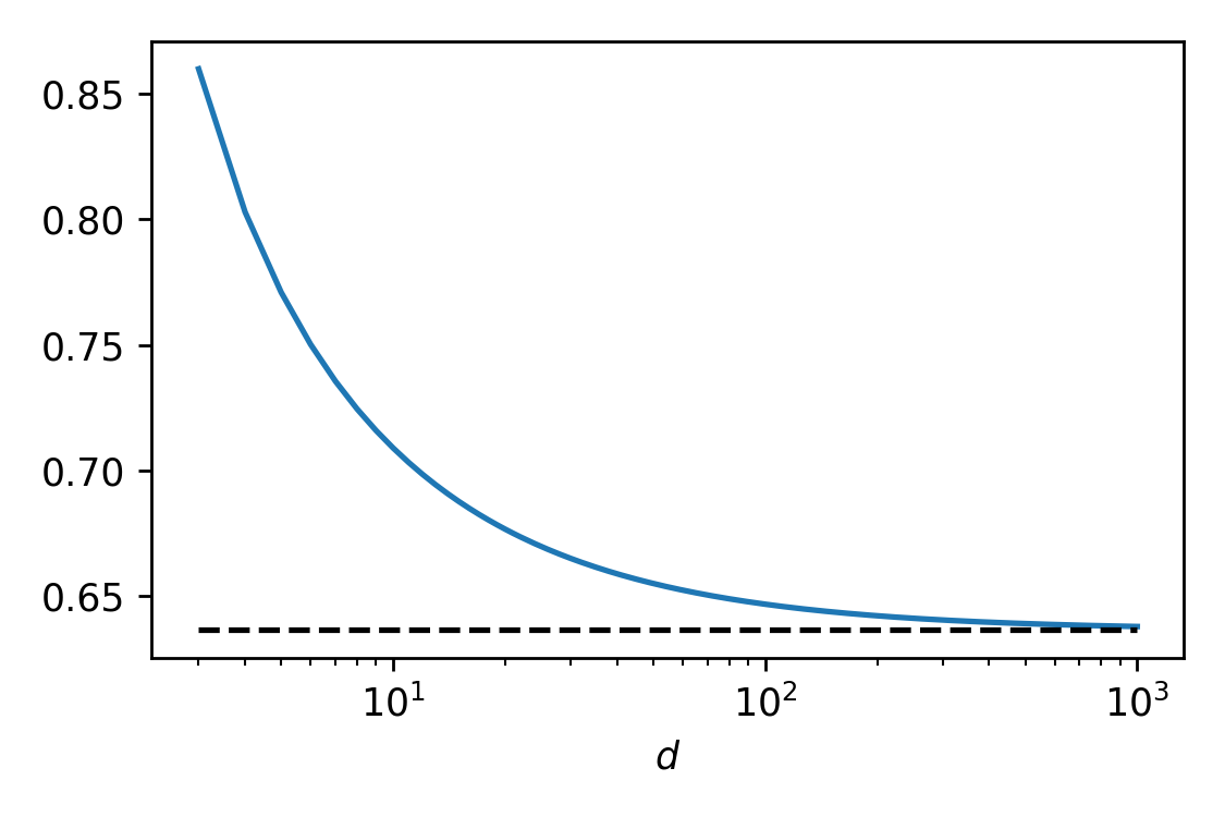
Figure 2: Convergence of the contraction rate estimate (5) to its asymptotic value. The blue line represents the value of (5) at each integer dimension $d=3,4,\dots,10^{3}$. The dashed black line marks the asymptotic rate estimate $2/\pi$.

In the limit $d\rightarrow\infty$, the rate estimate (5) simplifies to

$$\rho=\frac{1}{2\pi}\int_{0}^{2\pi}\absolutevalue{\cos(\omega)}\text{d}\omega=\frac{2}{\pi}\approx 0.64.$$

As can be seen in Figure 2, the rate estimate (5) takes some time to converge to this asymptotic rate estimate, only becoming visually indistinguishable from it when the dimension is in the order of hundreds or thousands.

Finally, we place our result in the broader context of GSSS performance. Specifically, we wish to emphasize that the dimension-stabilizing performance of GSSS for the uniform target is particularly remarkable because it fundamentally alters our understanding of how well GSSS can scale with increasing dimension: As already mentioned in Section 1, it was shown in [2] that GSSS is uniformly geometrically ergodic, with the explicit dependence of their convergence rate estimate $\rho<1$ on the dimension being rather moderate. However, it is well-known that convergence rate estimates obtained by the uniform geometric ergodicity framework are typically poor estimates of the (non-uniform) convergence rate corresponding to the spectral gap.

Moreover, intuitive considerations regarding the spectral gap of GSSS suggest a worse scaling with increasing dimension: If we consider targets that are highly concentrated around some point on the sphere, GSSS for these targets will mostly stay in the small region of high probability mass. Since $\mathbb{S}^{d-1}$ locally behaves like $\R^{d-1}$, GSSS in such settings will behave roughly like hit-and-run uniform slice sampling (cf. e.g. [9]) on $\R^{d-1}$. In [3] it was shown that the latter always performs worse than (ideal) uniform slice sampling in terms of its spectral gap. Furthermore, from [5, 10] it is known that uniform slice sampling in turn suffers from a curse of dimensionality for both light-tailed and heavy-tailed targets, with the one for light-tailed targets being relatively moderate (but already stronger than the one in [2, Theorems 15,26]) and the one for heavy-tailed targets being significantly stronger. Due to the sphere’s compactness, we suspect the poor dimension-scaling of uniform slice sampling for heavy-tailed targets to be largely irrelevant to the performance of GSSS. However, its moderate curse of dimensionality for light-tailed targets will, by our assessment, most likely also manifest itself in the performance of GSSS for highly concentrated targets. It is therefore encouraging to learn that GSSS can, in principle, work very well in arbitrarily high dimension.

References

- [1] Randal Douc, Eric Moulines, Pierre Priouret, and Philippe Soulier, Markov chains, Springer Series in Operations Research and Financial Engineering, Springer, Cham, 2018. MR 3889011
- [2] Michael Habeck, Mareike Hasenpflug, Shantanu Kodgirwar, and Daniel Rudolf, Geodesic slice sampling on the sphere, arXiv preprint arXiv:2301.08056v1, 2023.
- [3] Krzysztof Latuszyński and Daniel Rudolf, Convergence of hybrid slice sampling via spectral gap, arXiv preprint arXiv:1409.2709, 2014.
- [4] Oren Mangoubi and Aaron Smith, Rapid mixing of geodesic walks on manifolds with positive curvature, The Annals of Applied Probability 28 (2018), no. 4, 2501–2543. MR 3843835
- [5] Viacheslav Natarovskii, Daniel Rudolf, and Björn Sprungk, Quantitative spectral gap estimate and Wasserstein contraction of simple slice sampling, The Annals of Applied Probability 31 (2021), no. 2, 806–825. MR 4254496
- [6] Yann Ollivier, Ricci curvature of Markov chains on metric spaces, Journal of Functional Analysis 256 (2009), no. 3, 810–864. MR 2484937
- [7] Gareth O. Roberts and Jeffrey S. Rosenthal, The polar slice sampler, Stochastic Models 18 (2002), no. 2, 257–280. MR 1904830
- [8] Daniel Rudolf and Philip Schär, Dimension-independent spectral gap of polar slice sampling, arXiv preprint arXiv:2305.03685, 2023.
- [9] Daniel Rudolf and Mario Ullrich, Comparison of hit-and-run, slice sampler and random walk metropolis, Journal of Applied Probability 55 (2018), no. 4, 1186–1202. MR 3899935
- [10] Philip Schär, Wasserstein contraction and spectral gap of slice sampling revisited, arXiv preprint arXiv:2305.16984, 2023.
- [11] Philip Schär, Michael Habeck, and Daniel Rudolf, Gibbsian polar slice sampling, Proceedings of the 40th International Conference on Machine Learning, Proceedings of Machine Learning Research, vol. 202, PMLR, 2023, pp. 30204–30223.