Unsupervised Green Object Tracker (GOT) without Offline Pre-training

Abstract

Supervised trackers trained on labeled data dominate the single object tracking field for superior tracking accuracy. The labeling cost and the huge computational complexity hinder their applications on edge devices. Unsupervised learning methods have also been investigated to reduce the labeling cost but their complexity remains high. Aiming at lightweight high-performance tracking, feasibility without offline pre-training, and algorithmic transparency, we propose a new single object tracking method, called the green object tracker (GOT), in this work. GOT conducts an ensemble of three prediction branches for robust box tracking: 1) a global object-based correlator to predict the object location roughly, 2) a local patch-based correlator to build temporal correlations of small spatial units, and 3) a superpixel-based segmentator to exploit the spatial information of the target frame. GOT offers competitive tracking accuracy with state-of-the-art unsupervised trackers, which demand heavy offline pre-training, at a lower computation cost. GOT has a tiny model size ($<$3k parameters) and low inference complexity (around 58M FLOPs per frame). Since its inference complexity is between $0.1\%\sim 10\%$ of DL trackers, it can be easily deployed on mobile and edge devices.

I Introduction

Video object tracking is one of the fundamental computer vision problems [1] and finds applications in various applications such as autonomous driving [2, 3] and video surveillance [4]. Given the ground-truth bounding box of the object in the first frame of a test video, a single object tracker (SOT) predicts the object box in all subsequent frames. Most trackers follow the tracking-by-detection paradigm. That is, based on the object template obtained in the $(i-1)$th frame (i.e., the reference frame), a tracker conducts similarity matching over a search region at the $i$th frame (i.e., the target frame). This setting is used to reflect an online real-time tracking environment, where the data processing is applied to streaming video with a small memory buffer.

Research on SOT has a long history, which will be briefly reviewed in Sec. II. There are two major breakthroughs in SOT development. The first one lies in the use of the discriminative correlation filter (DCF) [5] and its variants. Based on handcrafted features (e.g., the histogram of oriented gradients (HOG) and colornames (CN) [6]) extracted from the reference template, DCF trackers estimate the location and size of the target template by examining the correlation (or similarity) between the reference template and the image content in the target search region. The second one arises by exploiting deep neural networks (DNNs) or deep learning (DL). Supervised and unsupervised DL trackers with pre-trained networks have been dominating in their respective categories in recent years. They are trained with large-scale offline pre-training data. The former has human-labeled object boxes throughout all frames, while the latter does not, in all training sequences.

There is a link between DCF and DL trackers. One representative branch of supervised DL trackers is known as the Siamese network, which maintains the template matching idea. On the other hand, DL trackers adopt the end-to-end optimization approach to derive powerful deep features for the matching purpose. Besides the backbone network, they incorporate several auxiliary subnetworks called heads, e.g., the classification head and the box regression head.

The superior tracking accuracy of supervised DL trackers is attributed to a huge amount of efforts in offline pre-training with densely labeled videos and images. In addition, the backbone network gets larger and larger from the AlexNet to the Transformer. Generally speaking, DL trackers demand a large model size and high computational complexity. The heavy computational burden hinders their practical applications in edge devices. For example, SiamRPN++ [7] has a model containing 54M parameters and takes 48.9G floating point operations (flops) to track one frame. To lower the high computational resource requirement, research has been done to compress the model via neural architecture search [8], model distillation [9], or networks pruning and quantization [10, 11, 12, 13, 14].

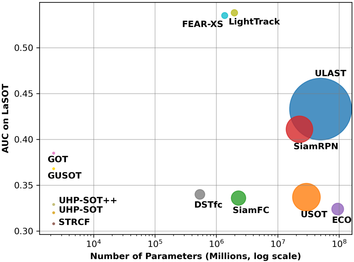
Figure 1: Comparison of object trackers in the number of model parameters (along the x-axis), the AUC performance (along the y-axis) and inference complexity in floating point operations (in circle sizes) with respect to the LaSOT dataset.

One recent research activity lies in reducing the labeling cost. Along this line, unsupervised DL trackers have been proposed to enable intelligent learning, e.g., [15, 16, 17, 18]. In the training process, they generate pseudo object boxes in initial frames, allow a tracker to track in both forward and backward directions, and enforce the cycle consistency. Various techniques have been proposed to adjust pseudo labels and improve training efficiency. Unsupervised DL trackers contain complicated networks needed for large-scale offline pre-training, leading to large model sizes. The state-of-the-art unsupervised DL tracker, ULAST [18], achieves comparable performance as top supervised DL trackers. As a modification of SiamRPN++, ULAST has a large model size and heavy computational complexity in inference.

Our research goal is to develop unsupervised, high-performance, and lightweight trackers, where lightweightness is measured in model sizes and inference computational complexity. Toward this objective, we have developed new trackers by extending DCF trackers. Examples include UHP-SOT [19], UHP-SOT++ [20] and GUSOT [21]. The extensions include an object recovery mechanism and flexible shape estimation in the face of occlusion and deformation, respectively. They improved the tracking accuracy of DCF trackers greatly while maintaining their lightweight advantage. These trackers were not only unsupervised but also demanded no offline pre-training. Furthermore, these trackers adopted a modular design for algorithmic transparency.

Based on the above discussion, we can categorize object trackers into three types according to their training strategies: A) supervised trackers, B) unsupervised trackers with offline pre-training, and C) unsupervised trackers without offline pre-training. In terms of training complexity, Type B has the highest training complexity while Type C has the lowest training complexity (which is almost none). We consider their representative trackers in Fig. 1:

• Type A: SiamFC, ECO, SiamRPN, LightTrack, DSTfc, and FEAR-XS;

• Type B: USOT and ULAST;

• Type C: STRCF, UHP-SOT, UHP-SOT++, GUSOT, and GOT.

We compare their characteristics in three aspects in the figure: tracking performance (along the y-axis), model sizes (along the x-axis), and inference complexity (in circle sizes).

The green object tracker (GOT) is a new tracker proposed in this work. It is called “green” due to its low computational complexity in both training and inference stages, leading to a low carbon footprint. There is an emerging research trend in artificial intelligence (AI) and machine learning (ML) by taking the carbon footprint into account. It is called “green learning” [22]. Besides sustainability, green learning emphasizes algorithmic transparency by adopting a modular design. GOT has been developed based on the green learning principle.

GOT conducts an ensemble of three prediction branches for robust object tracking: 1) a global object-based correlator to predict the object location roughly, 2) a local patch-based correlator to build temporal correlations of small spatial units, and 3) a superpixel-based segmentator to exploit the spatial information (e.g., color similarity and geometrical constraints) of the target frame. For the first and the main branch, GOT adopts GUSOT as the baseline. The outputs from three branches are then fused to generate the ultimate object box, where an innovative fusion strategy is developed.

GOT contains two novel ideas that have been neglected in the existing object tracking literature. They are elaborated below.

• The performance of the global correlator in the first branch degrades when the tracked object has severe deformation between two adjacent frames. The local patch-based correlator in the second branch is used to provide more flexible shape estimation and object re-identification. It is essential to implement the local correlator efficiently. It is formulated as a binary classification problem. It classifies a local patch into one of two classes - belonging to the object or the background.

• The tracking process usually alternates between the easy steady period and the challenging period as confronted with deformations and occlusion. The proposed fuser monitors the tracking quality and fuses different box proposals according to the tracking dynamics to ensure robustness against challenges while maintaining a reasonable complexity.

We evaluate GOT on five benchmarking datasets for thorough performance comparison. They are OTB2015, VOT2016, TrackingNet, LaSOT, and OxUvA. It is demonstrated by extensive experiments and ablation studies that GOT offers competitive tracking accuracy with state-of-the-art unsupervised trackers (i.e., USOT and ULAST), which demand heavy offline pre-training, at a lower computation cost. GOT has a tiny model size ($<$3k parameters) and low inference complexity (around 58M FLOPs per frame). Its inference complexity is between $0.1\%\sim 10\%$ of DL trackers. Thus, it can be easily deployed on mobile and edge devices. Furthermore, we discuss the role played by supervision and offline pre-training to shed light on our design.

The rest of this paper is organized as follows. Related work is reviewed in Sec. II. The GOT method is proposed in Sec. III. Experimental results are shown in Sec. IV. Concluding remarks are given in Sec. VI.

II Related Work

II-A DCF Trackers

Unsupervised DCF trackers without offline pre-training had been popular before the arrival of DL trackers. Given a reference template, DCF trackers conduct circulant patch sampling on the target frame and predict the location and size of the object template via regression. Quite a few DCF trackers with various regression objective functions or feature representations were proposed, e.g., [5, 23, 24, 25, 26, 27, 28, 29, 30]. Classic DCF trackers estimate the scale change by checking multiple scales. Yet, they are not flexible in adjusting the aspect ratio of the bounding box. Recently, DCF-based trackers such as UHP-SOT++ [20] and GUSOT [21] allow more flexible shape change by adopting low-cost segmentation techniques and exploiting motion residuals. The latter can facilitate object re-identification after tracking loss. Generally speaking, all DCF trackers meet the requirement of being an unsupervised lightweight solution without offline pre-training. The main concern is their poorer tracking accuracy as compared with modern DL trackers. Thus, the main task is how to boost the tracking performance with little extra cost in memory and computation. In this work, we adopt GUSOT [21] as the baseline of GOT since it has demonstrated good performance in tracking long videos.

II-B DL Trackers

II-B1 Offline Pre-training

The majority of high-performance DL trackers adopt offline pre-training on large-scale datasets, including still images [31, 32] and densely annotated videos [33, 34, 35, 36]. Modularized trackers use pre-trained convolutional neural networks (CNNs) as the feature extraction backbone [37, 38, 39]. End-to-end trackers need to finetune the backbone with auxiliary networks to be adapted to the tracking task [40, 41, 7, 42, 43, 44]. The transformer boosts the tracking accuracy of supervised DL trackers to a higher level [45, 46]. Although the power of offline pre-training with annotated boxes in tracking performance boosting is obvious, there are associated costs. First, it is a heavy burden to scale up the training data. Second, one needs to remove noise in newly sourced videos to obtain high-quality annotations. Third, the costly offline training process yields a large carbon footprint.

II-B2 Unsupervised Trackers

To address the high human labeling cost, researchers investigate ways to conduct offline pre-training with unlabeled data [15, 16, 17, 18]. As proposed in ResPUL [16], one idea is to train the backbone network offline with contrastive learning on static images and enhance the learning process with temporal sample mining. Another idea is to impose cycle consistency in offline pre-training. For example, UDT [15] proposed the cycle training method. It randomly crops patches in the first frame as object templates (or pseudo labels) and trains the tracker to track forward and then backward to yield a consistent object location in the initial frame. Later work put efforts into cleaning noisy pseudo labels and improving cycle training efficiency. Rather than random cropping on any video frame, USOT [17] detected moving objects using a dense optical flow and selected valid video segments to avoid influence from occlusion or out-of-view. It also expanded the cycle training interval. As the state-of-the-art unsupervised tracker, ULAST [18] applied a region mask to filter out possible contaminations from the non-object region and weigh the loss from pseudo labels of different quality. ULAST can achieve comparable performance against supervised trackers with a large network and high computational complexity. It demands large-scale offline pre-training and its training complexity is significantly higher than that of supervised trackers due to the extra cycle consistency requirement.

II-B3 Lightweight Trackers

The majority of DL trackers rely on powerful yet heavy backbones (e.g., CNNs or transformers). To deploy them on resource-limited platforms, efforts have been made in compressing a network without degrading its tracking accuracy. Various approaches have been proposed such as neural architecture search (NAS) [8], model distillation [9], network quantization [13], feature sparsification, channel pruning [14], or other specific designs to reduce the complexity of original network layers [11, 10, 12]. As a pioneering method, LightTrack [8] lays the foundation for later lightweight trackers. LightTrack adopted NAS to compress a large-size supervised tracker into its mobile counterpart. Its design process involved the following three steps: 1) train a supernet, 2) search for its optimal subnet, and 3) re-train and tune the subnet on a large number of training data. The inference complexity can be reduced to around 600M flops per frame at the end. Simply speaking, it begins with a well-designed supervised tracker and attempts to reduce the model size and complexity with re-training. Another example was proposed in [9]. It also conducted NAS to find a small network and used it to distill the knowledge of a large-size tracker via teacher-student training.

Our work is completely different from DL trackers as the proposed GOT does not have an end-to-end optimized neural network architecture. It adopts a modularized and interpretable system design. It is unsupervised without offline pre-training. It is proper to view GOT as a descent (or a modern version) of classic DCF trackers. Our main task in developing GOT is to identify the shortcomings of classic DCF trackers and find their remedies.

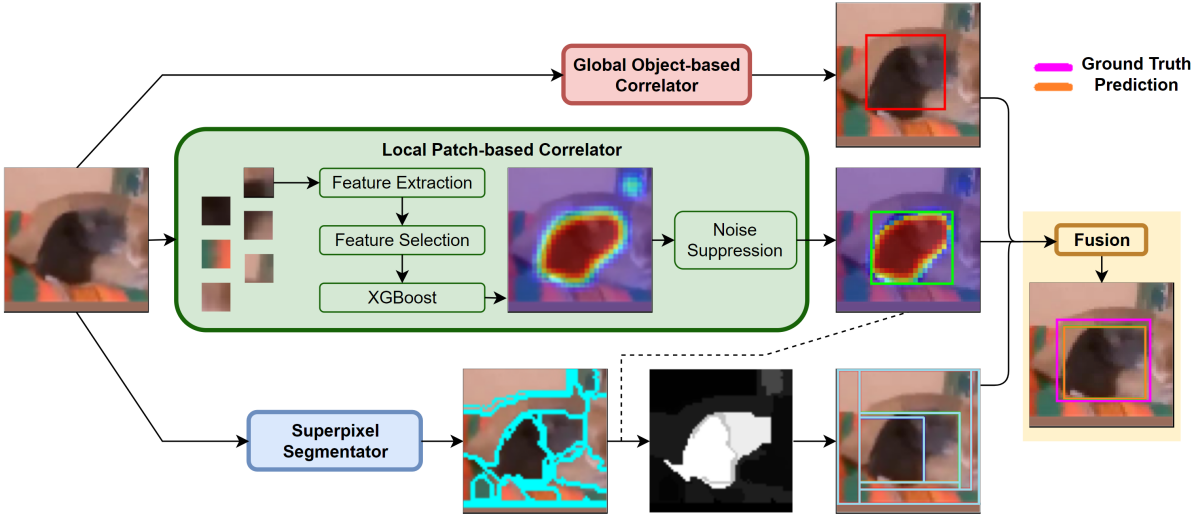
Figure 2: The system diagram of the proposed green object tracker (GOT). The global object-based correlator generates a rigid proposal, while the local patch-based correlator outputs a deformable box and a objectness score map which helps the segmentator calculate additional deformable boxes. These proposals are fused into one final prediction.

III Green Object Tracker (GOT)

The system diagram of the proposed green object tracker (GOT) is depicted in Fig. 2. It contains three bounding box prediction branches: 1) a global object-based correlator, 2) a local patch-based correlator applied to small spatial units, and 3) a superpixel segmentator. Each branch will offer one or multiple proposals from the input search region, and they will be fused to yield the final prediction. We use GUSOT [21] in the first branch and the superpixel segmentation technique [47] in the third branch. In the following, we provide a brief review of the first branch in Sec. III-A, and elaborate on the second branch in Sec. III-B. We do not spend any space on the superpixel segmentator since it is directly taken from [47]. Finally, we present the fusion strategy in Sec. III-D.

III-A Global Object-based Correlator

The GUSOT tracker is the evolved result of a series of efforts in enhancing the performance of lightweight DCF-based trackers. They include STRCF [28], UHP-SOT [19] and UHP-SOT++ [20]. STRCF adds a temporal regularization term to the objective function used for the regression of the feature map of an object template in a DCF tracker. STRCF can effectively capture the appearance change while being robust against abrupt errors. However, it generates only rigid predictions and cannot recover from the tracking loss. UHP-SOT enhances it with two modules: background motion modeling and trajectory-based box prediction. The former models background motion, conducts background motion compensation, and identifies the salient motion of a moving object in a scene. It facilitates the re-identification of the missing target after tracking loss. The latter estimates the new location and shape of a tracked object based on its past locations and shapes via linear prediction. The two modules can collaborate together to estimate the box aspect ratio change to some extent. UHP-SOT++ further improves the fusion strategy of different modules and conducts more extensive experiments on the effectiveness of each module on several tracking datasets.

Although STRCF, UHP-SOT, and UHP-SOT++ boost the performance of classic DCF trackers by a significant margin, their capability in flexible shape estimation and object re-identification is still limited. This is because they rely on the correlation between adjacent frames, while an object template is vulnerable to shape deformation and cumulative tracking errors in the long run. To improve the tracking performance in long videos, GUSOT examines the shape estimation problem and the object recovery problem furthermore. It exploits the spatial and temporal correlation by considering foreground and background color distributions. That is, colors in a search window are quantized into a set of primary color keys. They are extracted across multiple frames since they are robust against appearance change. These salient color keys can identify object/background locations with higher confidence. A low-cost graph-cut-based segmentation method can be used to provide the object mask. GUSOT can accommodate flexible shape deformation to a certain degree.

All above-mentioned trackers model the object appearance from the global view, i.e., using features of the whole object for the matching purpose. They provide robust tracking results when the underlying object is distinctive from background clutters without much deformation or occlusion. For this reason, we adopt the global object-based correlator in the first branch. The advanced version, GUSOT, is implemented in GOT.

III-B Local Patch-based Correlator

The local patch-based correlator analyzes the temporal correlation existing in parts of the tracked object. It is designed to handle object deformations more effectively. It is formulated as a binary classification problem. Given a local patch of size $8\times 8$, the binary classifier outputs its probability of being parts of the object or the background. This is a novel contribution of this work.

III-B1 Feature Extraction and Selection

The channel-wise Saab transform is an unsupervised representation learning method proposed in [48]. It is slightly modified and used to extract features of a patch here. We decompose a color input image into overlapping patches with a certain stride and subtract the mean color of each patch to obtain its color residuals. The mean color offers the average color of a patch. The color residuals are analyzed using the processing pipeline shown in Fig. 3, where the input consists of zero-mean RGB residual channels. We conduct the spectral principle component analysis (PCA) on RGB residuals to get three decorrelated channels denoted by P, Q and R channels. For each of them, another spatial PCA is conducted to reduce the feature dimension to $C$. The final feature vector is formed by concatenating of features of each color channel at each pixel. Note that spectral and spatial PCA kernels are learned at the initial frame only and shared among all remaining frames. Given the two PCA kernels, the computation described above can be easily implemented by convolutional layers of CNNs. Besides the Saab features, handcrafted features such as HOG and CN are also included for richer representation. Then, a feature selection technique called discriminant feature test (DFT) [49] is adopted to select a subset of discriminant features. The feature selection process is only conducted in the initial frame. Once the features are selected, they are kept and shared among later frames to reduce computational complexity.

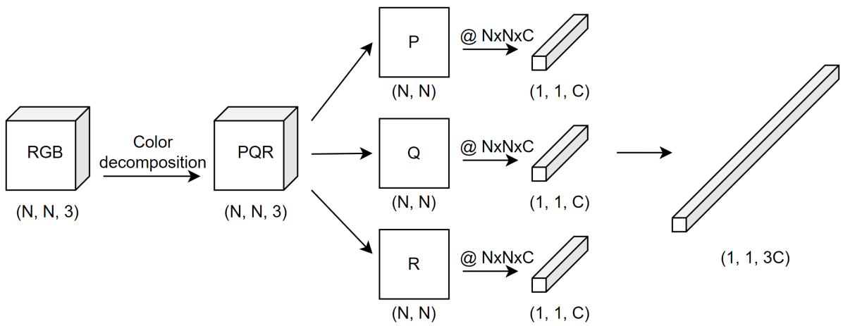
Figure 3: Channel-wise Saab transformation on color residuals of a patch of size $N\times N$.

III-B2 Patch Classification

If a patch is fully outside and inside the bounding box in the reference frame, it is assigned “0” and “1”, respectively. As for patches lying on the box boundary, they are not used in training to avoid confusion. Feature vectors and labels are used in an XGBoost classifier [50]. In the experiment, we set the tree number and the maximum tree depth to 40 and 4, respectively. These hyperparameters are determined via offline cross validation on a set of training videos. They can also be determined using samples in the initial frame. The predicted soft probability scores of patches in the search window of the target frame form a heat map which is called the objectness score map. Note that some patches inside the bounding box may belong to the background rather than the object, leading to noisy labels. To alleviate this problem, we adopt a two-stage training strategy. The first-stage classifier is trained using labels based on the patch location inside/outside of the bounding box in the reference frame. It is applied to patches in the target frame to produce soft probabilities. Then, the soft probabilities are binarized again to provide finetuned patch labels. Due to the feature similarity between true background patches and false foreground patches, their predicted soft labels should be closer and, as a result, finetuned labels are more reliable than initial labels. The second-stage classifier is trained using finetuned labels.

III-B3 From Heat Map to Bounding Box

To obtain a rectangular bounding box, we binarize the heat map and draw a tight enclosing box to obtain an objectness proposal. Due to noise around the object boundary, direct usage of the heat map does not yield stable box prediction. To overcome the problem, we smoothen the heat map and use it to weigh the raw heat map for noise suppression. Let $P_{t}\in\mathbf{R}^{H\times W}$, $S_{t-1}$, and $S_{t}$ denote the raw probability map of frame $t$, the template of frame $t-1$ and the updated template of frame $t$, respectively. Note that $S_{t-1}$ has been registered to align with $P_{t}$ via circulant translation. The processed heat map is expressed as

$$P_{t}^{*}=P_{t}\odot S_{t-1},$$ (1)

where $\odot$ is the element-wise multiplication for locations where $S_{t-1}$ has the objectness score below 0.5. Then, $S_{t}$ is updated by minimizing a cost function as follows:

$$S_{t}=\arg\min_{X}{\|X-P_{t}^{*}\|_{F}^{2}+\mu\|X-S_{t-1}\|_{F}^{2}},$$ (2)

where parameter $\mu$ controls the tradeoff between the updating rate and smoothness. Eq. (2) is a regularized least-squares problem. It has the closed-form solution

$$S_{t} =[P_{t}^{*},\mu S_{t-1}][I_{H},\mu I_{H}]^{\dagger}$$ (3)

$$=[P_{t}^{*},\mu S_{t-1}]([1,\mu]\otimes I_{H})^{\dagger}$$

$$=[P_{t}^{*},\mu S_{t-1}]([1,\mu]^{\dagger}\otimes I_{H}^{\dagger})$$

$$=[P_{t}^{*},\mu S_{t-1}]([1,\mu]^{\dagger}\otimes I_{H})$$

$$=[P_{t}^{*},\mu S_{t-1}]([\frac{1}{1+\mu^{2}},\frac{\mu}{1+\mu^{2}}]^{T}\otimes I_{H})$$

$$=\frac{1}{1+\mu^{2}}P_{t}^{*}+\frac{\mu^{2}}{1+\mu^{2}}S_{t-1},$$

where ${\dagger}$, $\otimes$, and $I_{H}$ are the Moore–Penrose pseudoinverse, the Kronecker product and the $H\times H$ identity matrix, respectively. We use several examples to visualize the evolution of templates over time in Figure 4.

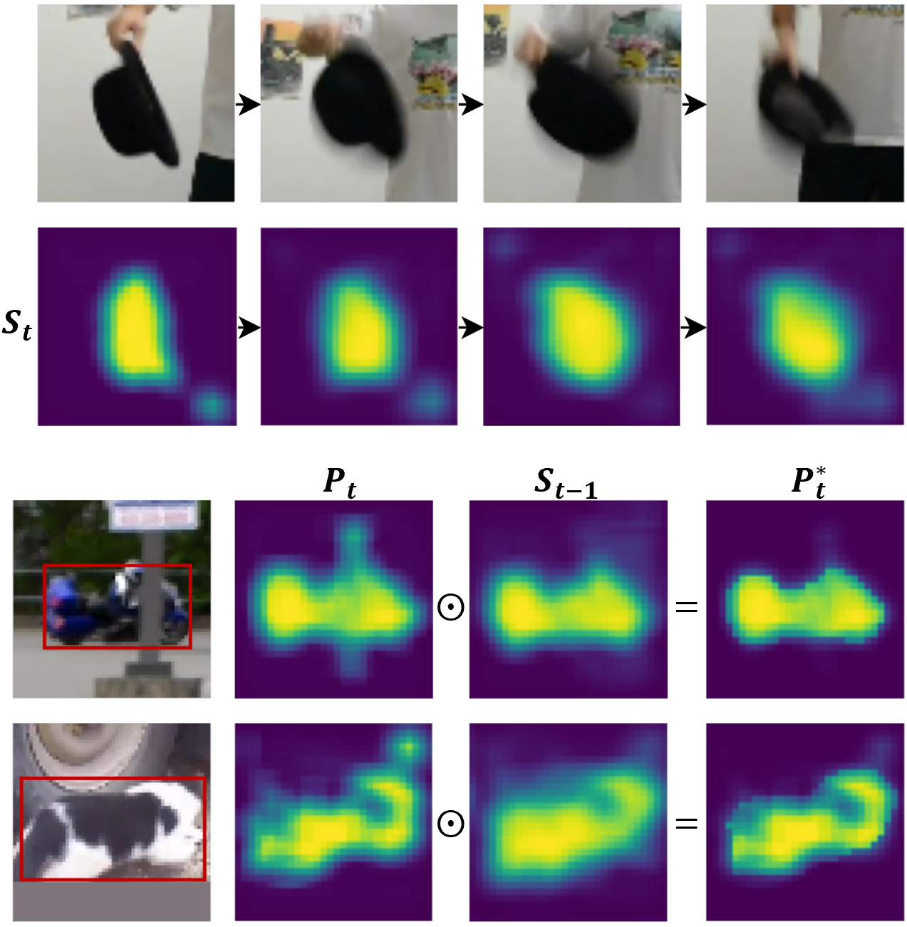
Figure 4: (Top) Visualization of the evolution of templates over time and (bottom) visualization of the noise suppression effect in the raw probability map based on Eq. (1).

III-B4 Classifier Update

Since the object appearance may change over time, the classifier needs to be updated to adapt to a new environment. The necessity of classifier update can be observed based on the classification performance. The heat map is expected to span the object template reasonably well. If it deviates too much from the object template, an update is needed. As shown in Fig. 5, regions of higher probability (marked by warm colors) tend to shrink when there are new object appearances (in the top example) or they may go out of the box when new background appears (in the bottom example). Once one of such phenomena is observed, the classifier should be retrained using samples from an earlier frame of high confidence and those from the current frame. The retraining cost is low because of the tiny size of the classifier.

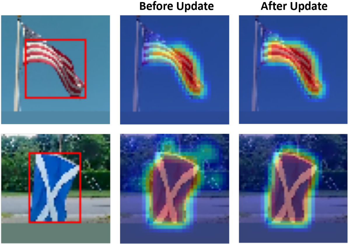
Figure 5: Proper updating helps maintain decent classification quality.

III-C Superpixel Segmentation

For the first and the second branches, we exploit temporal correlations of the object and background across multiple frames. In the third branch, we consider spatial correlation in the target frame and perform the unsupervised segmentation task. Superpixel segmentation has been widely studied for years. It offers a mature technique to generate a rough segmentation mask. However, to group superpixels into a connected group, an algorithm usually checks the appearance similarity and geometric connectivity, which can be expensive. In our case, the heat map provides a natural grouping guidance. When we overlay the heat map and superpixel segments, each segment gets an averaged probability score. Then, we can group segments by considering various probability thresholds and draw multiple box proposals, as shown in Fig. 2. They are called superpixel proposals.

III-D Fusion of Proposals

There are three types of proposals in GOT: 1) the DCF proposal $x_{dcf}$ from the global object-based correlator, 2) the objectness proposal $x_{obj}$ from the local patch-based correlator, and 3) the superpixel proposals $\chi_{spp}=\{x_{spp,i}|i=1,..,N\}$ from the superpixel segmentator. While $\chi_{spp}$ contains multiple proposals by grouping different segments, the most valuable one can be selected by evaluating the intersection-over-union (IoU) as

$$x^{*}_{spp}=\arg\max_{x\in\chi_{spp}}{\text{IoU}(x,x_{dcf})+\lambda\text{IoU}(x,x_{obj})},$$ (4)

where $\lambda$ is an adaptive weight calculated from $\text{IoU}(x_{dcf},x_{obj})$. It lowers the contribution of poor heat maps. In the following, we first present two fusion strategies that combine multiple proposals into one final prediction and then elaborate on tracking quality control and object re-identification.

III-D1 Two Fusion Strategies

According to the difficulty level of the tracking scenario, one final box bounding is generated from these proposals with a simple or an advanced fusion strategy.

Simple Fusion. During an easy tracking period without obvious challenges, multiple proposals tend to agree well with each other. Then, we adopt a simple strategy based on IoU and probability values. The current tracking status is considered as easy if

$$\min_{x_{i},x_{j}\in{x_{dcf},x_{obj},x_{spp}}}{\text{IoU}(x_{i},x_{j})}\geq\alpha,$$

where $\alpha$ is the threshold to distinguish good and poor alignment. Under this condition, we first fuse flexible proposals $x_{obj}$ and $x_{spp}$ and then choose from the flexible proposal and the rigid proposal $x_{dcf}$ via the following steps:

• Choose from $x_{obj}$ and $x_{spp}$ by finding $x_{df}^{*}=\arg\max_{x}{\text{IoU}(x,x_{dcf})}$.

• Choose from $x_{df}^{*}$ and $x_{dcf}$. Stick to $x_{dcf}$ if it has a larger averaged probability score inside the box and the size of $x_{def}^{*}$ changes too rapidly when compared with the previous prediction.

Advanced Fusion. When multiple proposals differ a lot, it is nontrivial to select the best one just using IoU or probability distribution. Instead, we fuse the information from different sources with the following optimization process. A rough foreground mask $\mathbf{I^{*}}$ is derived by searching the optimal 0/1 label assignment to pixels in the image. Let $x$ and $l_{x}$ denote the pixel location and its label. The mask, $\mathbf{I^{*}}$, can be estimated using the Markov Random Field (MRF) optimization:

$$\mathbf{I^{*}}=\arg\min_{\mathbf{I}}{\sum_{x}{\rho(x,l_{x})}+\sum_{\{x,y\}\in\aleph}{w_{xy}\|l_{x}-l_{y}\|}},$$ (5)

where $\aleph$ is the four-connected neighborhood, the second term assigns penalties to neighboring points that do not have the same labels, the weight $w_{xy}$ is calculated from the color difference between $x$ and $y$, and

$$\rho(x,l_{x})=-\log{p_{color}(l_{x}|x)}-\log{p_{obj}(l_{x}|x)}$$ (6)

treats the negative log-likelihood of $x$ being assigned to the foreground color and that of $x$ being foreground in terms of objectness. The former is modeled by the Gaussian mixtures while the latter comes from the classification results. The rough mask in Eq. (5) takes color, objectness, and connectivity into account to find the most likely label assignment. While the solution could be improved iteratively, we only run one iteration since the result is good enough to serve as the rough mask. Next, to fuse proposals, we select the one that gets the highest IoU with the wrapping box of the rough mask. If the advanced fusion fails, we go back to the simple fusion as a backup. The overall fusion strategy that consists of both simple and advanced fusion schemes is summarized in Algorithm 1.

Algorithm 1 Fusion of Multiple Proposals

0:  $x_{dcf}$, $x_{obj}$, $\chi_{spp}$, $\alpha$, $P_{t}^{*}$

0:  final prediction $x_{t}$

  $x_{spp}\leftarrow\arg\max_{x\in\chi_{spp}}{\text{IoU}(x,x_{dcf})+\lambda\text{IoU}(x,x_{obj})}$

  $flag\leftarrow\{\min_{x_{i},x_{j}\in{x_{dcf},x_{obj},x_{spp}}}{\text{IoU}(x_{i},x_{j})}\}\geq\alpha$

  if $flag$ is false then

     generate box $x_{mrf}$ from MRF mask

     if success then

        return  $x_{t}\leftarrow\arg\max_{x\in x_{dcf},x_{obj},\chi_{spp}}{\text{IoU}(x,x_{mrf})}$

     end if

  end if

  $x_{df}^{*}\leftarrow\arg\max_{x\in{x_{obj},x_{spp}}}{\text{IoU}(x,x_{dcf})}$

  $S_{P_{t}^{*}}(x_{df}^{*})\leftarrow$ averaged probability inside $x_{df}^{*}$

  $S_{P_{t}^{*}}(x_{dcf})\leftarrow$ averaged probability inside $x_{dcf}$

  if $x_{df}^{*}$ is stable or $S_{P_{t}^{*}}(x_{df}^{*})>S_{P_{t}^{*}}(x_{dcf})$ then

     return  $x_{t}\leftarrow x_{df}^{*}$

  end if

  return  $x_{t}\leftarrow x_{dcf}$

III-D2 Tracking Quality Control

For rigid objects with rigid motion, the global object-based correlator can provide a fairly good prediction. The template matching similarity score of DCF is usually high. The local patch-based correlator usually helps in the face of challenges such as background clutters and occlusions. However, due to the complicated nature of local patch classification, its proposal may be noisy. Detection and removal of noisy proposals in the second branch are important to good tracking performance in general. To solve this issue, we monitor the quality of the heat map and may discard noisy proposals until classification gets stable again. The flowchart of tracking quality control is depicted in Fig. 6. After the heat map is obtained, we check whether the high probability region is too small or too large and whether it contains several unconnected blobs. All of them indicate that the local patch-based correlator is not stable. Thus, its proposal is discarded. Once the problem is resolved, the heat map becomes stable, and the objectness proposal shall have small variations in height and width. Then, we can turn on the shape estimation functionality (i.e., the local patch-based correlator in the second branch) and conduct the fusion of all proposals.

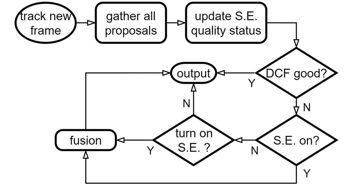
Figure 6: Management of different tools for tracking, where S.E. denotes the shape estimation function provided by the second branch.

An exemplary sequence is illustrated in Fig. 7. In the beginning, the tracking process is smooth and the simple fusion is sufficient. Then, when some challenges appear and multiple proposed boxes do not align, we turn to the advanced MRF fusion. When there is severe background clutter or occlusion that confuses the classifier in the second branch, the DCF proposal is adopted directly until the turbulence goes away. Then, the process repeats until the end of the video.

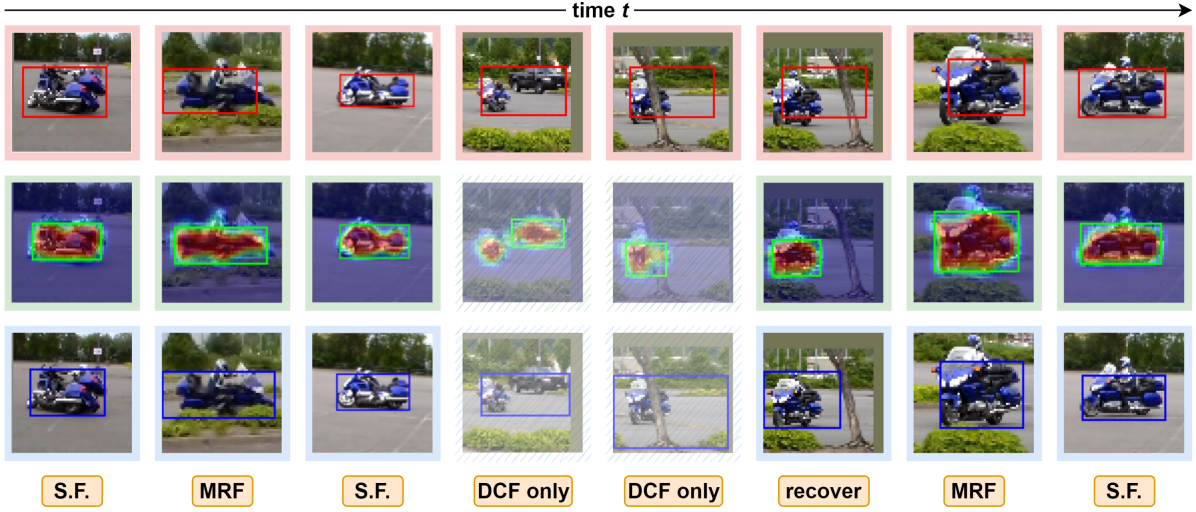
Figure 7: The fusion strategy (given in the fourth row, where S.F. stands for simple fusion) changes with tracking dynamics over time. The DCF proposal, the objectness proposal, and the superpixel proposal are given in the first, second, and third rows, respectively. The sequence is motorcycle-9 from LaSOT and the object is the motorbike.

III-D3 Object Re-identification

Besides shape estimation, the objectness proposal can be used for object re-identification after tracking loss. Given the current DCF proposal and the motion proposal that covers the most motion flow and possibly contains the lost foreground object, GUSOT selects one of the two via trajectory stability and color/template similarity. However, GUSOT is not general enough to cover all cases. The objectness score provides an extra view of the appearance similarity with timely updated object information, and it helps recover the object quickly.

Given a candidate box proposal $x$ with center $x_{ct}$, its averaged objectness score $S_{obj}(x)$ inside the box, the feature representation $f(x)$ of the region, and the DCF template $f_{t-1}$, the scoring function for this candidate can be calculated as

$$S(x)=\beta_{1}\langle f(x),f_{t-1}\rangle+\beta_{2}S_{obj}(x)-\beta_{3}\|x_{ct}-\hat{x}_{t,ct}\|^{2},$$ (7)

where $\hat{x}_{t}$ is the linear prediction of the box center based on past predictions, $\beta_{1}$ and $\beta_{3}$ are positive constants to adjust the magnitudes of all terms to the same level, $\beta_{2}$ is a positive adaptive weight that assigns lower contributions for poorer probability maps. An ideal candidate box is expected to have high template similarity, high objectness score, and with a small translation from the last prediction. Then, we can choose from the DCF proposal and the motion proposal by selecting the one with a higher evaluation score to re-identify the lost object.

IV Experiments

IV-A Experimental Setup

IV-A1 Performance Metrics

The one-pass-evaluation (OPE) protocol is adopted for all trackers in performance benchmarking unless specified otherwise. The metrics for tracking accuracy include: the distance precision (DP) and the area-under-curve (AUC). DP measures the center precision at the 20-pixel threshold to rank different trackers, and AUC is calculated using the overlap precision curve. For model complexity, we consider two metrics: the model size and the computational complexity required to predict the target object box from the reference one on average. The latter is also called the inference complexity per frame. The model size is the number of model parameters. The inference complexity per frame is measured by the number of (multiplication or add) floating point operations (flops).

IV-A2 Benchmarking Object Trackers

We compare GOT with the following four categories of trackers.

• supervised lightweight DL trackers: LightTrack [8], DSTfc [9], and FEAR-XS [12].

• supervised DL trackers: SiamFC [40], ECO [39], and SiamRPN [41].

• unsupervised DL trackers: LUDT [51], ResPUL [16], USOT [17], and ULAST [18].

• unsupervised DCF trackers: KCF [23], SRDCF [6], and STRCF [28].

For unsupervised DL trackers, we use the models trained from scratch for comparison if they are available.

IV-A3 Tracking Datasets

We conduct performance evaluations of various trackers on four datasets.

• OTB2015 [52]. It contains 100 videos with an average length of 598 frames. The dataset was released in 2015. Many video sequences are of lower resolution.

• VOT2016 [53]. It contains 60 video sequences with an average length of 358 frames. It has a significant overlap with the OTB2015 dataset. One of its purposes is to detect the frequency of tracking failures. Different from the OPE protocol, once a failure is detected, the baseline experiment re-initializes the tracker.

• TrackingNet [35]. It is a large-scale dataset for object tracking in the wild. Its testing set consists of 511 videos with an average length of 442 frames.

• LaSOT [54]. It is the largest single object tracking dataset by far. It has 280 long testing videos with 685K frames in total. The average video length is 2000+ frames. Thus, it serves as an important benchmark for measuring long-term tracking performance.

TABLE I: Comparison of tracking accuracy and model complexity of representative trackers of four categories on four tracking datasets. Some numbers for model complexity are rough estimations due to the lack of detailed description of network structures and/or public domain codes. Furthermore, the complexity of some algorithms is related to built-in implementation and hardware. OPT and UT are abbreviations for offline pre-training and unsupervised trackers, respectively. The top 3 runners among all unsupervised trackers (i.e., those in the last two categories) are highlighted in red, green, and blue, respectively.

				OTB2015		VOT16	TrackingNet		LaSOT
Tracker	OPT/UT	Flops ($\downarrow$)	No. of Params.($\downarrow$)	DP ($\uparrow$)	AUC ($\uparrow$)	EAO($\uparrow$)	DP($\uparrow$)	AUC($\uparrow$)	DP ($\uparrow$)	AUC ($\uparrow$)
LightTrack[8]	✓/$\times$	530 M (9X)	1.97 M (896X)	-	66.2	-	69.5	72.5	53.7	53.8
DSTfc[9]	✓/$\times$	1.23 G (21X)	0.54 M (246X)	76.1	57.3	-	51.2	56.2	-	34.0
FEAR-XS[12]	✓/$\times$	478 M (8X)	1.37 M (623X)	-	-	-	-	-	54.5	53.5
SiamFC[40]	✓/$\times$	2.7 G (47X)	2.3 M (1046X)	77.1	58.2	23.5	53.3	57.1	33.9	33.6
ECO[39]	✓/$\times$	1.82 G (31X)	95 M (43201X)	90.0	68.6	37.5	48.9	56.1	30.1	32.4
SiamRPN[41]	✓/$\times$	9.23 G (159X)	22.63 M (10291X)	85.1	63.7	34.4	-	-	38.0	41.1
LUDT[51]	✓/✓	-	-	76.9	60.2	23.2	46.9	54.3	-	26.2
ResPUL[16]	✓/✓	2.65 G (46X)	1.445 M (657X)	-	58.4	26.3	48.5	54.6	-	-
USOT[17]	✓/✓	$>$14 G (241X)	29.4 M (13370X)	79.8	58.5	35.1	55.1	59.9	32.3	33.7
ULAST[18]	✓/✓	$\gtrapprox$50 G (862X)	$\gtrapprox$50 M (22738X)	81.1	61.0	-	-	-	40.7	43.3
KCF[23]	$\times$/✓	-	-	69.6	48.5	19.2	41.9	44.7	16.6	17.8
SRDCF[6]	$\times$/✓	-	-	78.1	59.3	24.7	45.5	52.1	21.9	24.5
STRCF[28]	$\times$/✓	-	-	86.6	65.8	27.9	-	-	29.8	30.8
GOT (Ours)	$\times$/✓	$\approx$58 M (1X)	2199 (1X)	87.6	65.4	26.8	52.6	56.3	38.8	38.5

IV-A4 Implementation Details

In the implementation, each region of interest is warped into a $60\times 60$ patch with an object that takes around $32\times 32$ pixels. The XGBoost classifier in the local correlator has 40 trees with the maximum depth set to 4. Parameters $\alpha=0.7$ and $\mu=5$ are used in the fuser. The first branch (i.e., the global correlator), the combined second and third branches (i.e., the local correlator and the superpixel segmentator), and the fuser runs at 15 FPS, 5 FPS, and 15 FPS on one Intel(R) Core(TM) i5-9400F CPU, respectively. The speed can be further improved via code optimization and parallel programming.

IV-B Performance Evaluation

We compare the performance of GOT with four categories of trackers on four datasets in Table I. Trackers are grouped based on their categories. From top to down, they are supervised lightweight DL trackers, supervised DL trackers, unsupervised DL trackers, and unsupervised DCF trackers, respectively. Our proposed GOT belongs to the last category. We have the following observations.

OTB2015. GOT has the best performance in DP and the second best performance in AUC among unsupervised trackers on this dataset. One explanation is that DL trackers are trained on high-resolution videos and they do not generalize well to low-resolution videos. GOT is robust against different resolutions since its HoG and CN features are stable to ensure a higher successful rate of the template matching idea.

VOT2016. It adopts the expected average overlap (EAO) metric to evaluate the overall performance of a tracker. EAO considers both accuracy and robustness. The observation on this dataset reveals that the advantages of the local correlator branch are not obvious on very short videos since the tracker gets corrected automatically if its IoU is lower than a threshold. Yet, GOT still ranks third among unsupervised trackers (i.e., the last two categories) with a tiny model (of 2.2K parameters) and much lower inference complexity by 3 to 5 orders of magnitude.

TrackingNet. The ground-truth box is provided for the first frame only. The performance of GOT is evaluated by an online server. GOT ranks second among unsupervised trackers. Its performance is also comparable with almost all supervised DL trackers (except LightTrack).

LaSOT. GOT ranks second among unsupervised trackers. It even has better performance than some supervised trackers such as DSTfc while maintaining a much smaller model size and lower computational complexity.

IV-C Comparison Among Lightweight Trackers

We compare the design methods and training costs of GOT and three lightweight DL trackers in Table II. The lightweight DL trackers conduct the neural architecture search (NAS) or model distillation/optimization to reduce the model size and inference complexity. As shown in Table I, LightTrack achieves even higher tracking accuracy than large models. Besides NAS, FEAR-XS [12] adopts several special tools such as depth-wise separable convolutions and increases the number of object templates to lower complexity while maintaining high accuracy. Although DSTfc has the smallest model size among the three, its model size is still larger than that of GOT by two orders of magnitude. Furthermore, the tracking performance of GOT is better than that of DSTfc in three datasets. As to the training cost, all three lightweight DL trackers need pre-training on millions of labeled frames while GOT does not require any as shown in the last column of Table I. The superiority of LightTrack in accuracy does have a cost, including long pre-training, architecture search and fine-tuning. Finally, it is worth mentioning that GOT is more transparent in its design. Thus, its source of tracking errors can be explained and addressed. In contrast, the failure of lightweight DL trackers is difficult to analyze. It could be overcome by adding more pre-training samples and repeating the whole design process one more time.

TABLE II: Comparison of design methods and pre-training costs of GOT and three lightweight DL trackers.

Trackers	Design Methods	# of Pre-Training Boxes
LightTrack[8]	NAS	$\approx 10$M
DSTfc[9]	NAS, model distillation	$\approx 2$M
FEAR-XS [12]	NAS, network optimization	$\approx 13$M
GOT (Ours)	fusion of 3 branches	0

IV-D Long-term Tracking Capability

To examine GOT’s capability in long-term tracking, we test it on the test set of the OxUva dataset [55]. OxUva contains 166 long test videos under the tracking-in-the-wild setting. The object to be tracked disappears from the field of view in around one half of video frames. Trackers need to report whether the object is present or absent and give the object box when it is present. The ground-truth labels are hidden, and the tracking results are evaluated on a competition server. Since the competition is not maintained any longer, we cannot submit our results for official evaluation. For this reason, we use predictions from the leading tracker LTMU [56] as the pseudo labels for performance evaluation below. There are three major evaluation metrics: the true positive rate (TPR), the true negative rate (TNR) and the maximum geometric mean (MaxGM), which is calculated as

$$\text{MaxGM}=\max_{0\leq p\leq 1}{\sqrt{(1-p)\cdot\text{TPR}\cdot((1-p)\cdot\text{TNR}+p)}},$$ (8)

where TPR stands for the fraction of presented objects that are predicted as present and located with a tight bounding box, and TNR represents the fraction of absent objects that are correctly reported as absent.

We compare the above performance metrics of GOT against three lightweight long-term trackers, KCF [23] (the long-term version), TLD [57] and FuCoLoT [58], in Table III. TLD and FuCoLoT are equipped with a re-detection mechanism to find the object after loss. We see that GOT achieves the highest TPR because of its accurate box predictions. FuCoLoT and GOT do not provide present/absent predictions so their TNR values are zero. In GOT^∗, the object is claimed to be absent if the similarity score of template matching is lower than a threshold, which is set to $0.1$ in the experiment. Then, KCF and GOT^∗ have comparable performance in TNR. Finally, GOT^∗ has the best performance in MaxGM. The above design indicates that the similarity score in GOT is a simple yet effective indicator of the object status. The effect of various threshold values on GOT^∗ is illustrated in Fig. 8. As the threshold grows from $0$ to $0.15$, its TPR decreases slowly while its TNR increases quickly. The optimal threshold for the MaxGM metric is around $0.1$.

TABLE III: Performance comparison of GOT and GOT^∗ against three lightweight long-term trackers, KCF (the long-term version), TLD and FuCoLoT, on the OxUvA dataset, where the best performance is shown in red. KCF and TLD are implemented in OpenCV.

	KCF	TLD	FuCoLoT	GOT	GOT∗
TPR ($\uparrow$)	0.165	0.142	0.353	0.425	0.351
TNR ($\uparrow$)	0.872	0.095	0	0	0.751
MaxGM ($\uparrow$)	0.380	0.198	0.297	0.326	0.514

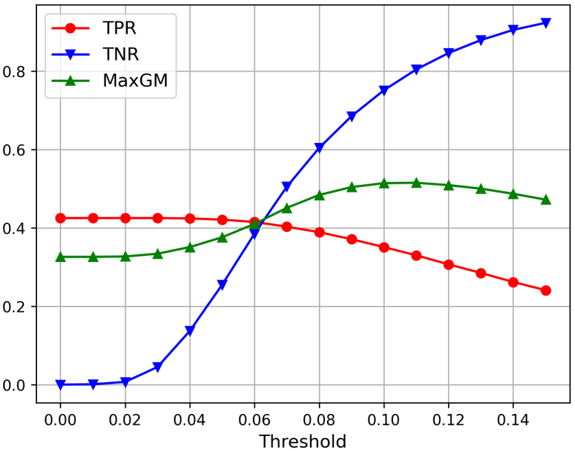
Figure 8: The TPR, TNP and MaxGM values of GOT^∗ at different present/absent threshold values against the OxUva dataset.

IV-E Attribute-based Performance Evaluation

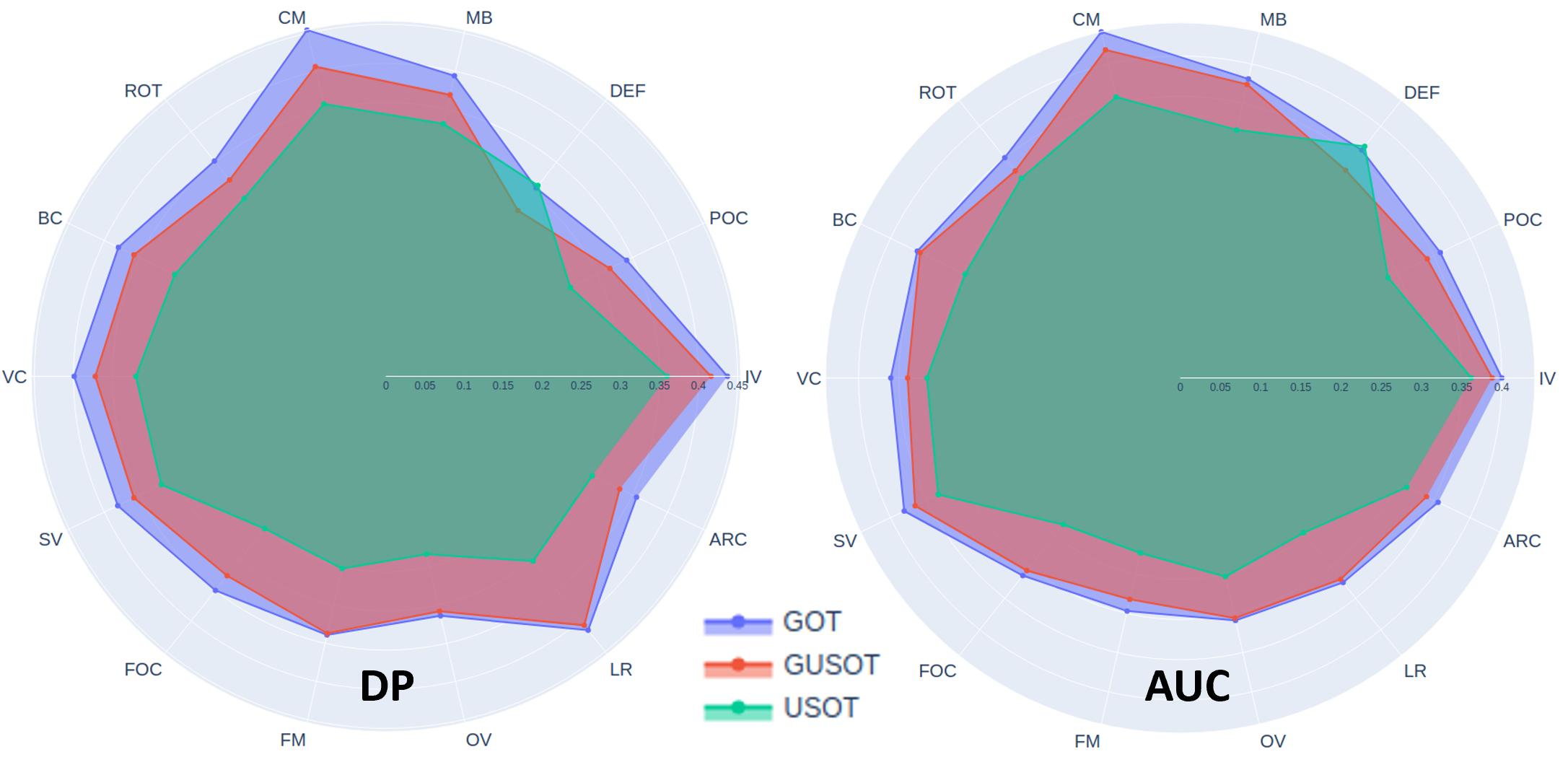
Figure 9: Attribute-based evaluation of GOT, GUSOT and USOT on LaSOT in terms of DP and AUC, where attributes of interest include the aspect ratio change (ARC), background clutter (BC), camera motion (CM), deformation (DEF), fast motion (FM), full occlusion (FOC), illumination variation (IV), low resolution (LR), motion blur (MB), occlusion (OCC), out-of-view (OV), partial occlusion (POC), rotation (ROT), scale variation (SV) and viewpoint change (VC).

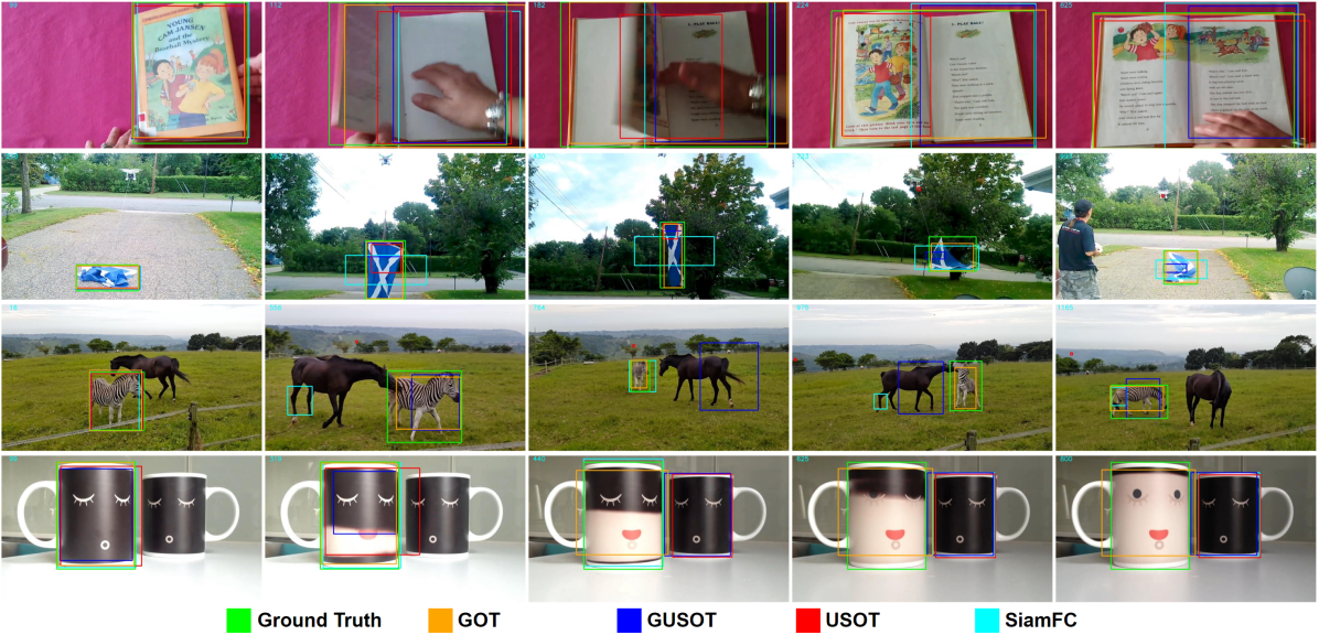
Figure 10: Comparison of the tracked object boxes of GOT, GUSOT, USOT, and SiamFC for four video sequences from LaSOT (from top to bottom: book, flag, zebra, and cups). The initial appearances are given in the first (i.e., leftmost) column. The tracking results for four representative frames are illustrated.

To shed light on the strengths and weaknesses of GOT, we conduct the attribute-based study among GOT, the GUSOT baseline, and USOT, which is an unsupervised DL tracker, on the LaSOT dataset. DPs and AUCs with respect to different challenging attributes are presented in Fig. 9. GUSOT outperforms USOT in all aspects except deformation (DEF) due to its limited segmentation-based shape adaptation capability. With the help of the local correlator branch and the powerful fuser, GOT performs better than GUSOT and has comparable performance with USOT, which is equipped with a box regression network, in DEF. For the same reason, GOT outperforms GUSOT in other DEF-related attributes such as viewpoint change (VC), rotation (ROT), and aspect ratio change (ARC). Another improvement lies is camera motion (CM), where the local correlator contributes to better object re-identification. GOT has the least improvement in low resolution (LR). It appears that both the local correlator and the superpixel segmentation cannot help the GUSOT baseline much in this case. Lower video resolutions make the local features (say, around the boundaries) less distinguishable from each other.

As discussed above, GOT adapts to the new appearance and shape well against the DEF challenge. Representative frames of four video sequences from LaSOT are illustrated in Fig. 10 as supporting evidence. All tracked objects have severe deformations. For the first sequence of turning book pages, GOT covers the whole book correctly. For the second sequence of a flag, GOT can track the flag accurately. For the third sequence of a zebra, object re-identification helps GOT relocate the prediction to the correct place once the object is free from occlusion. For the fourth sequence of two cups, GOT is robust against background clutters. In contrast, other trackers fail to catch the new appearance or completely lose the object.

IV-F Insights into GOT’s New Ingredients

GOT has two new ingredients: 1) the local correlator in the 2nd branch and 2) the fuser to combine the outputs from all three branches. We provide further insights into them below.

IV-F1 Local Correlator

We compare the performance of GOT under different settings on the LaSOT dataset in Table IV. The settings include:

• With or without the local correlator branch;

• With or without classifier update;

• With or without object re-identification.

We see from the table that a “plain” local correlator already achieves a substantial improvement in DP. Classifier update and/or object re-identification improve more in AUC but less in DP. This is because deformation tends to happen around object boundaries and the change of the object center is relatively slow. On the other hand, the addition of classifier update and object re-identification helps improve the quality of the objectness map for better shape estimation. In addition, the improvement from object re-identification indicates the frequent object loss in long videos and the effective contribution of the objectness score. Both classifier update and object re-identification are needed to achieve the best performance.

TABLE IV: Performance comparison of GOT under different settings on the LaSOT dataset, where the best performance is shown in red. The ablation study includes: 1) with or without the local correlator branch; 2) with or without classifier update; 3) with or without object re-identification.

L.C.B.	Clf. update	Re-idf.	DP ($\uparrow$)	AUC ($\uparrow$)
			36.1	36.8
✓			38.0	37.5
✓	✓		38.2	38.0
✓		✓	38.2	37.9
✓	✓	✓	38.8	38.5

To study the necessity of quality checking and maintenance in the classification system of the local correlator branch, we compare the tracking accuracy of three settings in Table V, where object re-identification is turned off in all settings. Without the shape estimation on-off scheme, the tracker simply stops the shape estimation function after failures. The performance drops, which reveals the frequent occurrence of challenges even in the early/middle stage of videos and the importance of quality checking. Noise suppression helps boost the tracking accuracy furthermore since it alleviates abrupt box changes due to noise around the object border.

TABLE V: Ablation study of the classification system in the local correlator branch in GOT on LaSOT under three settings, where the best performance is shown in red.

Shape Estimation On-Off	Noise Suppression	DP ($\uparrow$)	AUC ($\uparrow$)
✓		37.6	37.8
	✓	36.5	36.5
✓	✓	38.2	38.0

IV-F2 Fuser

The threshold parameter, $\alpha$, in Algorithm 1 is used to choose between the simple fusion or the MRF fusion. To study its sensitivity, we select a subset of 10 sequences from LaSOT and turn on shape estimation in most frames. The mean IoU and the center error between the ground truth and the prediction change are plotted as functions of the threshold value in Fig. 11. The optimal threshold range is between 0.7 and 0.9 since it has lower center errors and higher IoUs. Choosing a lower threshold means that we conduct the simple fusion. This is consistent with the proposed fusion strategy. That is, the simple fusion should be only used when different proposals are close to each other. Pure simple and MRF fusion strategies have their own weaknesses such as the limited selection ability in the simple fusion and errors around boundaries in the MRF fusion. Proper collaboration between them can boost the performance.

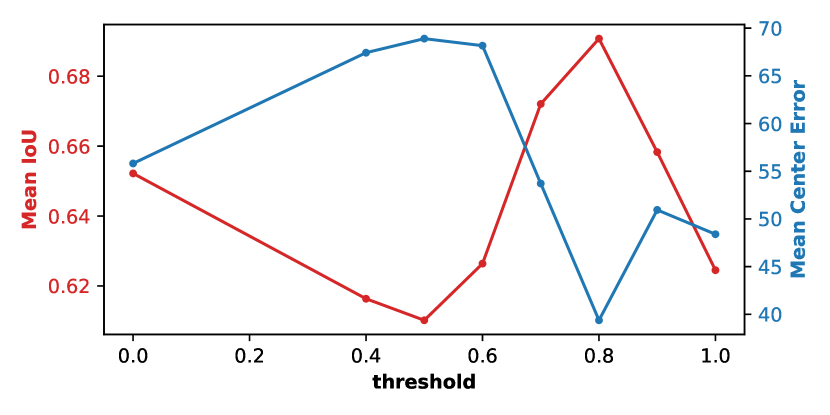
Figure 11: Mean IoU (the higher the better) and center error (the lower the better) on the selected subset with different fusion thresholds. The subset from LaSOT includes book-10, bus-2, cat-1, crocodile-14, flag-5, flag-9, gorilla-6, person-1, squirrel-19, mouse-17.

V Discussion on GOT’s Limitations

To analyze the limitations of GOT and gain a deeper understanding of the contributions of supervision and offline pre-training, we compare the performance of GOT and three DL trackers on the LaSOT dataset in Fig. 12. The three benchmarking trackers are SiamRPN++ (a supervised DL tracker), USOT (an unsupervised DL tracker), and SiamFC (a supervised DL tracker that does not have a regression network as the previous two DL trackers). The regression network is offline pre-trained. The left subfigure depicts the success rate as a function of different overlap thresholds. The right subfigure shows the AUC values as a function of different video lengths with the full length normalized to one.

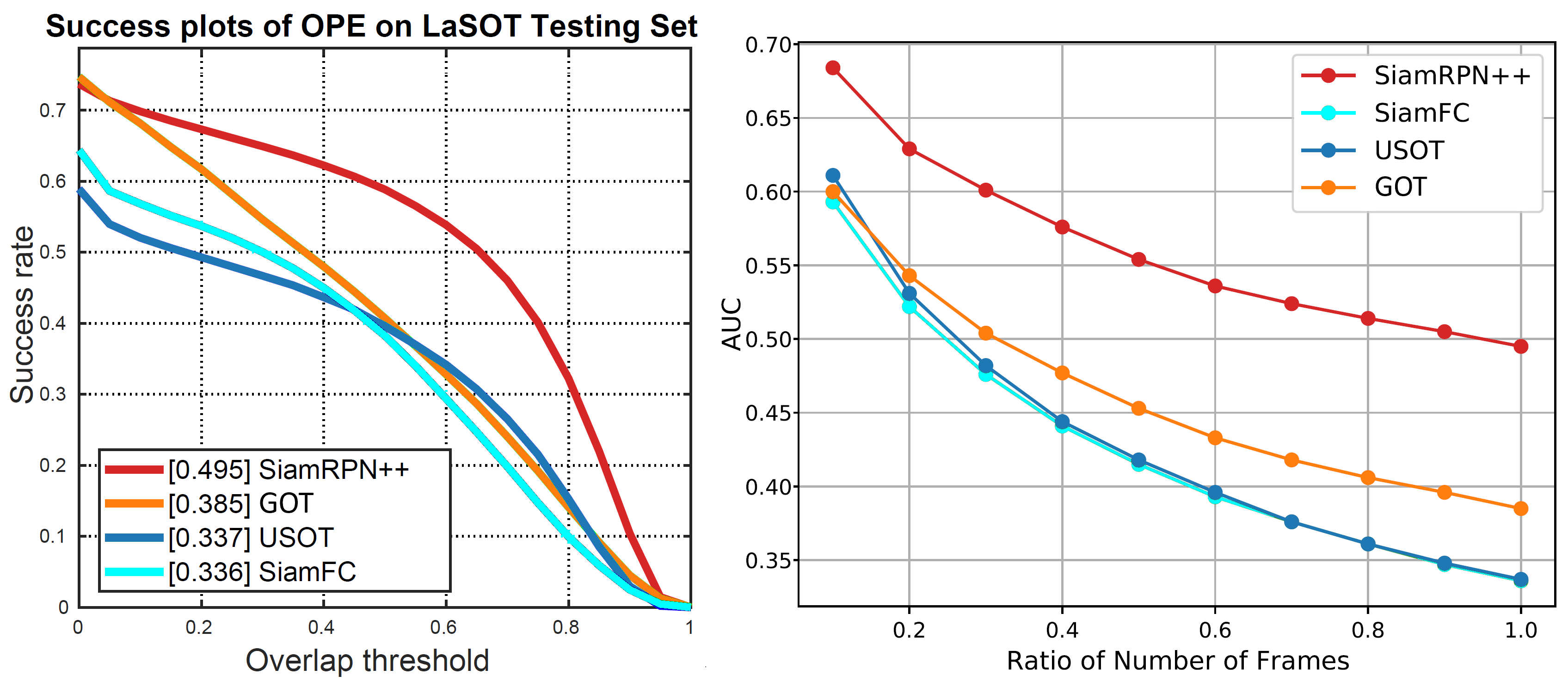
Figure 12: Performance comparison between GOT (orange), SiamRPN++ (red), SiamFC (cyan), and USOT (blue) on LaSOT in terms of the success rate plot (left) and the AUC plot.

SiamRPN++ has the best performance among all. It is attributed to both supervision and offline pre-training. GOT ranks second in most situations except for the following cases. GOT is slightly worse than USOT when the overlap threshold is higher or at the beginning part of videos. It is conjectured that GOT can achieve decent shape estimation but it may not be as effective as the offline pre-trained regression network used by USOT in a tighter condition, i.e., a higher overlap threshold or a shorter tracking memory. It is amazing to see that GOT outperforms SiamFC across all thresholds and all video lengths. This shows the importance of the regression network in DL trackers.

To verify the above conjecture, we conduct the deformation-related attribute study in a shorter tracking memory setting in Fig. 13, where only the first 10% of all frames (i.e., the ratio of frame numbers is 0.1) is examined. GOT is better than SiamFC in most attributes and worse than SiamRPN++ and USOT. The superiority of SiamFC over GOT in DEF and ROT indicates the power of supervision in locating the object.

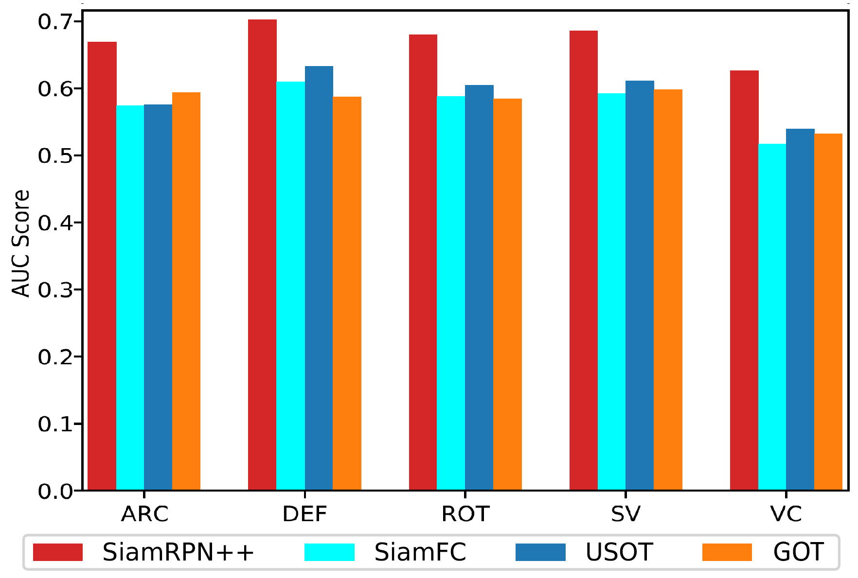
Figure 13: Deformation-related attribute study on LaSOT for the first 10% frames in videos.

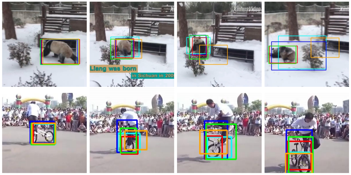
Figure 14: Two tracking examples from LaSOT: bear-4 (top) and bicycle-2 (bottom), with boxes of the ground truth (green), SiamRPN++ (red), SiamFC (cyan), USOT (blue), and GOT (orange), respectively.

We dive into two sequences where GOT’s attributes are poorer and show the tracking results in Fig. 14. As shown in these examples, GOT has difficulty in handling the following cases: (1) the object has similar local features with the background, such as the panda in the top sequence; and (2) the object under tracking does not have a tight shape, such as the bike in the bottom sequence. For the first case, the local patch-based correlator in GOT can only capture low-level visual similarities. It cannot distinguish the black color of the panda and the background. For the second case, the bounding box contains background patches inside, which become false positive samples. Besides, the object has a few small individual parts whose representations are not stable to reflect the appearance of the full object.

The motion may help if the object has obvious movement in the scene. However, it may not help much if the object moves slowly or overlaps with another object. These difficulties can be alleviated with supervision or pre-training. That is, if a learning model is trained with a rich set of object boxes, it can avoid such mistakes more easily. As for the gap between supervised pre-training and unsupervised pre-training, unsupervised methods use pseudo boxes generated randomly or from the optical flow that usually contains noise. Thus, the offered supervision is not as strong as ground truth labels. This explains why USOT cannot distinguish between the panda and the bush and fails to exclude the human body from the bike while SiamRPN++ does a good job.

Supervised DL trackers usually do not distinguish different tracking scenarios but tune a model to handle all cases to achieve high accuracy. Their high computational complexity, large model sizes and heavy demand on training data are costly. In contrast, the proposed GOT system with no offline pre-training can achieve decent tracking performance on general videos. Possible ways to enhance the performance of lightweight trackers include the design of better classifiers that have a higher level of semantic meaning and more powerful regressors for better fusion of predictions from various branches.

VI Conclusion and Future Work

A green object tracker (GOT) with a small model size, low inference complexity and high tracking accuracy was proposed in this work. GOT contains a novel local patch-based correlator branch to enable more flexible shape estimation and object re-identification. Furthermore, it has a fusion tool that combines prediction outputs from the global object-based correlator, the local patch-based correlator, and the superpixel-based segmentator according to tracking dynamics over time. Extensive experiments were conducted to compare the tracking performance of GOT and state-of-the-art DL trackers. We hope that this work could shed light on the role played by supervision and offline pre-training and provide new insights into the design of effective and efficient tracking systems.

Several future extensions can be considered. It is desired to develop ways to identify different tracking scenarios since this information can be leveraged to design a better tracking system. For example, it can adopt tools of different complexity to strike a balance between model complexity and tracking performance. Second, it can adopt different fusion strategies to combine outputs from multiple decision branches for more flexible and robust tracking performance.

Appendix A Model Size and Complexity Analysis of GOT

The number of model parameters and the computational complexity analysis of the proposed GOT system are analyzed. For the latter, we compute the floating point operations (flops) of the optimal implementation. Whenever it is applicable, we offer the time complexity and provide a rough estimation based on the running time on our local machine. The complexity analysis is conducted for tracking a new frame in the inference stage. Regardless of the original size of the frame, the region of interest is always warped into a $L_{B}\times L_{B}=60\times 60$ patch. The major components of GOT include the global object-based correlator (i.e., the DCF tracker), the local patch-based correlator (i.e., the classification pipeline), the superpixel-based segmentator, and the Markov Random Field (MRF) optimizer in the fuser.

Global Object-based Correlator. The DCF tracker involves template matching via FFT and template updating via regression. The template (feature map) dimension used in GOT is $(M,N,D)=(50,50,42)$. The complexity of template updating is $\mathcal{O}(DMN\log{MN})$, where $DMN\log{MN}\approx 1.19$M. The complexity of template matching is at the same level. Furthermore, there is a background motion modeling module in GUSOT to capture salient moving objects in the scene. The location of a certain point $(x_{t},y_{t})$ is estimated from its location in frame $t-1$ via the following affine transformation,

$$x_{t} = a_{0}x_{t-1}+b_{0}y_{t-1}+c_{0},$$ (9)

$$y_{t} = a_{1}x_{t-1}+b_{1}y_{t-1}+c_{1}.$$ (10)

It is applied to every pixel in frame $I_{t-1}$ to get an estimation $\hat{I}_{t}$ of frame $I_{t}$. Then, the motion residual map is calculated as

$$\Delta I=|\hat{I}_{t}-I_{t}|.$$ (11)

The maximum dimension of $\Delta I$ is $(H,W)=(720,480)$ as images of a larger size are downsampled. Flops for the affine transformation and the residual map calculation are $8*H*W+H*W\approx 3.11$M.

Local Patch-based Correlator. An input image of size $60\times 60$ is decomposed into overlapping blocks of size $8\times 8$ with a stride equal to 2, which generates $((60-8)/2+1)^{2}=729$ blocks for features extraction. For Saab feature extraction, we apply the one-layer Saab transform with filters of size $5\times 5$ and stride equal to 1. We keep the top 4 AC kernels from each of the PQR channels. Thus, there are 3 DC color responses of size $3\times 1\times 1$, and 12 AC responses of size $5\times 5\times 1$. After feature extraction, we apply the DFT feature selection method to reduce the feature dimension to 50. Hence, the number of parameters is calculated as $3\times 3\textit{ (color kernels)}+12\times 25\textit{ (Saab kernels)}+50\textit{ (DFT feature selection index)}=359.$ Since the Saab feature extraction process can be implemented as 3D convolutions as in neural networks, we follow the flops calculation there to compute the model flops for the Saab transform. For a general 3D convolution with $C_{i}$ input channels, $C_{o}$ filters of spatial size $K_{h}\times K_{w}$ and output spatial size of $H_{o}\times W_{o}$, the flops is calculated as

$$F=(2\times C_{i}\times K_{h}\times K_{w})\times H_{o}\times W_{o}\times C_{o}.$$ (12)

If the filter is a mean filter, the complexity is further reduced as

$$F =(C_{i}\times K_{h}\times K_{w})\times H_{o}\times W_{o}\times C_{o}.$$ (13)

As given in Table VI, the flops in computing the Saab features with filter size $5\times 5$ at stride 1 for a block of size $8\times 8\times 3$ is 11952. Then, the complexity for 729 blocks is around 8.713M. We run this feature extraction process at most two times at each frame.

TABLE VI: Flops of the Saab feature extraction for one spatial block of size $8\times 8$.

Steps	$C_{i}$	$K_{h}$	$K_{w}$	$H_{o}$	$W_{o}$	$C_{o}$	Flops
Get mean color	1	5	5	4	4	3	1200
RGB2PQR	3	1	1	8	8	3	1152
Saab on P	1	5	5	4	4	4	3200
Saab on Q	1	5	5	4	4	4	3200
Saab on R	1	5	5	4	4	4	3200
Total							11952

TABLE VII: The model size and the computational complexity of the whole GOT system.

Module	Num. of Params.	MFlops
Global Correlator	0	37.11
Local Correlator	2,199	18.12
Super-pixel segmentation	0	1.13
MRF	0	1.20
Total	2,199	57.56

TABLE VIII: The estimated flops for some special algorithmic modules.

Algorithmic Modules	Complexity	MFlops
2D FFT&IFFT	$\mathcal{O}(L_{B}^{2}\log{L_{B}})$	0.072
GMM	-	1.634
DCF template related	$\mathcal{O}(DMN\log{MN})$	34
Super-pixel segmentation	$\mathcal{O}(L_{B}^{2}\log{L_{B}})$	1.132

The XGBoost classifier has $N_{tree}=40$ trees with the maximum depth $d_{M}=4$ (i.e., there are at most four tree levels excluding the root). The maximum number of leaf nodes and parent nodes are $N_{l}=2^{d_{M}}$ and $N_{p}=2^{d_{M}}-1$, respectively. Hence, the number of parameters is bounded by $N_{tree}\times(2\times N_{p}+N_{l})=40\times(2\times 15+16)=1840$. The inference for 729 samples costs $d_{M}\times N_{tree}\times 729=4*40*729\approx 0.117$M flops. The complexity of spatial alignment via 2D FFT/IFFT is $\mathcal{O}(L_{B}^{2}\log{L_{B}})$. $L_{B}^{2}\log_{2}{L_{B}}\approx 0.021$M. The element-wise operation to get suppressed map takes $L_{B}\times L_{B}=3600$ flops. The template update costs around $3\times L_{B}\times L_{B}=10800$ flops.

Felzenszwalb Superpixel Segmentator. The complexity of the superpixel segmentation algorithm is $\mathcal{O}(L_{B}^{2}\log{L_{B}})$, which roughly takes 1.13 MFlops.

MRF. The adopted Markov Random Field optimizer has one iteration only. Given an input image of size $(L_{B},L_{B},C)=(60,60,3)$, it first learns the GMM models for foreground and background colors, respectively, so that the foreground/background likelihood can be calculated at each pixel. Then, around 20 element-wise matrix operations are conducted to calculate the rough assignment of pixel labels. The flops for matrix operations are $20*60*60=0.072M$.

We summarize the model size (in the number of model parameters) and the overall complexity (in flops) in Table VII. Our tracker has 2,199 model parameters and roughly 57.56 MFlops. It is worthwhile to point out that the actual complexity of some special modules such as FFT depend on the hardware implementation and optimization. Some of them are given in Table VIII.

References

- [1] S. Javed, M. Danelljan, F. S. Khan, M. H. Khan, M. Felsberg, and J. Matas, “Visual object tracking with discriminative filters and siamese networks: a survey and outlook,” IEEE Transactions on Pattern Analysis and Machine Intelligence, 2022.
- [2] K.-H. Lee and J.-N. Hwang, “On-road pedestrian tracking across multiple driving recorders,” IEEE Transactions on Multimedia, vol. 17, no. 9, pp. 1429–1438, 2015.
- [3] J. Janai, F. Güney, A. Behl, A. Geiger et al., “Computer vision for autonomous vehicles: Problems, datasets and state of the art,” Foundations and Trends® in Computer Graphics and Vision, vol. 12, no. 1–3, pp. 1–308, 2020.
- [4] J. Xing, H. Ai, and S. Lao, “Multiple human tracking based on multi-view upper-body detection and discriminative learning,” in 2010 20th International Conference on Pattern Recognition. IEEE, 2010, pp. 1698–1701.
- [5] D. S. Bolme, J. R. Beveridge, B. A. Draper, and Y. M. Lui, “Visual object tracking using adaptive correlation filters,” in 2010 IEEE computer society conference on computer vision and pattern recognition. IEEE, 2010, pp. 2544–2550.
- [6] M. Danelljan, G. Hager, F. Shahbaz Khan, and M. Felsberg, “Learning spatially regularized correlation filters for visual tracking,” in Proceedings of the IEEE international conference on computer vision, 2015, pp. 4310–4318.
- [7] B. Li, W. Wu, Q. Wang, F. Zhang, J. Xing, and J. Yan, “Siamrpn++: Evolution of siamese visual tracking with very deep networks,” in Proceedings of IEEE/CVF Computer Vision and Pattern Recognition, 2019, pp. 4282–4291.
- [8] B. Yan, H. Peng, K. Wu, D. Wang, J. Fu, and H. Lu, “Lighttrack: Finding lightweight neural networks for object tracking via one-shot architecture search,” in Proceedings of the IEEE/CVF Conference on Computer Vision and Pattern Recognition, 2021, pp. 15 180–15 189.
- [9] J. Shen, Y. Liu, X. Dong, X. Lu, F. S. Khan, and S. Hoi, “Distilled siamese networks for visual tracking,” IEEE Transactions on Pattern Analysis and Machine Intelligence, vol. 44, no. 12, pp. 8896–8909, 2021.
- [10] P. Blatter, M. Kanakis, M. Danelljan, and L. Van Gool, “Efficient visual tracking with exemplar transformers,” in Proceedings of the IEEE/CVF Winter Conference on Applications of Computer Vision, 2023, pp. 1571–1581.
- [11] X. Chen, B. Kang, D. Wang, D. Li, and H. Lu, “Efficient visual tracking via hierarchical cross-attention transformer,” in European Conference on Computer Vision. Springer, 2022, pp. 461–477.
- [12] V. Borsuk, R. Vei, O. Kupyn, T. Martyniuk, I. Krashenyi, and J. Matas, “Fear: Fast, efficient, accurate and robust visual tracker,” in European Conference on Computer Vision. Springer, 2022, pp. 644–663.
- [13] I. Jung, M. Kim, E. Park, and B. Han, “Online hybrid lightweight representations learning: Its application to visual tracking,” arXiv preprint arXiv:2205.11179, 2022.
- [14] S. Aggarwal, T. Gupta, P. K. Sahu, A. Chavan, R. Tiwari, D. K. Prasad, and D. K. Gupta, “On designing light-weight object trackers through network pruning: Use cnns or transformers?” in ICASSP 2023-2023 IEEE International Conference on Acoustics, Speech and Signal Processing (ICASSP). IEEE, 2023, pp. 1–5.
- [15] G. Wang, Y. Zhou, C. Luo, W. Xie, W. Zeng, and Z. Xiong, “Unsupervised visual representation learning by tracking patches in video,” in Proceedings of IEEE/CVF Computer Vision and Pattern Recognition, 2021, pp. 2563–2572.
- [16] Q. Wu, J. Wan, and A. B. Chan, “Progressive unsupervised learning for visual object tracking,” in Proceedings of IEEE/CVF Computer Vision and Pattern Recognition, 2021, pp. 2993–3002.
- [17] J. Zheng, C. Ma, H. Peng, and X. Yang, “Learning to track objects from unlabeled videos,” in Proceedings of the IEEE/CVF International Conference on Computer Vision, 2021, pp. 13 546–13 555.
- [18] Q. Shen, L. Qiao, J. Guo, P. Li, X. Li, B. Li, W. Feng, W. Gan, W. Wu, and W. Ouyang, “Unsupervised learning of accurate siamese tracking,” in Proceedings of IEEE/CVF Computer Vision and Pattern Recognition, 2022, pp. 8101–8110.
- [19] Z. Zhou, H. Fu, S. You, C. C. Borel-Donohue, and C.-C. J. Kuo, “UHP-SOT: An unsupervised high-performance single object tracker,” in 2021 International Conference on Visual Communications and Image Processing (VCIP). IEEE, 2021, pp. 1–5.
- [20] Z. Zhou, H. Fu, S. You, C.-C. J. Kuo et al., “UHP-SOT++: An unsupervised lightweight single object tracker,” APSIPA Transactions on Signal and Information Processing, vol. 11, no. 1, 2022.
- [21] Z. Zhou, H. Fu, S. You, and C.-C. J. Kuo, “Gusot: Green and unsupervised single object tracking for long video sequences,” in 2022 IEEE 24th International Workshop on Multimedia Signal Processing (MMSP). IEEE, 2022, pp. 1–6.
- [22] C.-C. J. Kuo and A. M. Madni, “Green learning: Introduction, examples and outlook,” Journal of Visual Communication and Image Representation, p. 103685, 2022.
- [23] J. F. Henriques, R. Caseiro, P. Martins, and J. Batista, “High-speed tracking with kernelized correlation filters,” IEEE transactions on pattern analysis and machine intelligence, vol. 37, no. 3, pp. 583–596, 2014.
- [24] M. Danelljan, G. Hager, F. Shahbaz Khan, and M. Felsberg, “Convolutional features for correlation filter based visual tracking,” in Proceedings of the IEEE international conference on computer vision workshops, 2015, pp. 58–66.
- [25] M. Danelljan, G. Häger, F. S. Khan, and M. Felsberg, “Discriminative scale space tracking,” IEEE transactions on pattern analysis and machine intelligence, vol. 39, no. 8, pp. 1561–1575, 2016.
- [26] M. Danelljan, A. Robinson, F. S. Khan, and M. Felsberg, “Beyond correlation filters: Learning continuous convolution operators for visual tracking,” in European conference on computer vision. Springer, 2016, pp. 472–488.
- [27] L. Bertinetto, J. Valmadre, S. Golodetz, O. Miksik, and P. H. Torr, “Staple: Complementary learners for real-time tracking,” in Proceedings of the IEEE conference on computer vision and pattern recognition, 2016, pp. 1401–1409.
- [28] F. Li, C. Tian, W. Zuo, L. Zhang, and M.-H. Yang, “Learning spatial-temporal regularized correlation filters for visual tracking,” in Proceedings of the IEEE conference on computer vision and pattern recognition, 2018, pp. 4904–4913.
- [29] T. Xu, Z.-H. Feng, X.-J. Wu, and J. Kittler, “Learning adaptive discriminative correlation filters via temporal consistency preserving spatial feature selection for robust visual object tracking,” IEEE Transactions on Image Processing, vol. 28, no. 11, pp. 5596–5609, 2019.
- [30] Y. Li, C. Fu, F. Ding, Z. Huang, and G. Lu, “Autotrack: Towards high-performance visual tracking for uav with automatic spatio-temporal regularization,” in Proceedings of IEEE/CVF Computer Vision and Pattern Recognition, 2020, pp. 11 923–11 932.
- [31] J. Deng, W. Dong, R. Socher, L.-J. Li, K. Li, and L. Fei-Fei, “Imagenet: A large-scale hierarchical image database,” in 2009 IEEE conference on computer vision and pattern recognition. Ieee, 2009, pp. 248–255.
- [32] T.-Y. Lin, M. Maire, S. Belongie, J. Hays, P. Perona, D. Ramanan, P. Dollár, and C. L. Zitnick, “Microsoft coco: Common objects in context,” in Computer Vision–ECCV 2014: 13th European Conference, Zurich, Switzerland, September 6-12, 2014, Proceedings, Part V 13. Springer, 2014, pp. 740–755.
- [33] O. Russakovsky, J. Deng, H. Su, J. Krause, S. Satheesh, S. Ma, Z. Huang, A. Karpathy, A. Khosla, M. Bernstein et al., “Imagenet large scale visual recognition challenge,” International journal of computer vision, vol. 115, pp. 211–252, 2015.
- [34] E. Real, J. Shlens, S. Mazzocchi, X. Pan, and V. Vanhoucke, “Youtube-boundingboxes: A large high-precision human-annotated data set for object detection in video,” in proceedings of the IEEE Conference on Computer Vision and Pattern Recognition, 2017, pp. 5296–5305.
- [35] M. Muller, A. Bibi, S. Giancola, S. Alsubaihi, and B. Ghanem, “Trackingnet: A large-scale dataset and benchmark for object tracking in the wild,” in Proceedings of the European conference on computer vision (ECCV), 2018, pp. 300–317.
- [36] L. Huang, X. Zhao, and K. Huang, “Got-10k: A large high-diversity benchmark for generic object tracking in the wild,” IEEE transactions on pattern analysis and machine intelligence, vol. 43, no. 5, pp. 1562–1577, 2019.
- [37] C. Ma, J.-B. Huang, X. Yang, and M.-H. Yang, “Hierarchical convolutional features for visual tracking,” in Proceedings of the IEEE international conference on computer vision, 2015, pp. 3074–3082.
- [38] Y. Qi, S. Zhang, L. Qin, H. Yao, Q. Huang, J. Lim, and M.-H. Yang, “Hedged deep tracking,” in Proceedings of the IEEE conference on computer vision and pattern recognition, 2016, pp. 4303–4311.
- [39] M. Danelljan, G. Bhat, F. Shahbaz Khan, and M. Felsberg, “Eco: Efficient convolution operators for tracking,” in Proceedings of the IEEE conference on computer vision and pattern recognition, 2017, pp. 6638–6646.
- [40] L. Bertinetto, J. Valmadre, J. F. Henriques, A. Vedaldi, and P. H. Torr, “Fully-convolutional siamese networks for object tracking,” in European conference on computer vision. Springer, 2016, pp. 850–865.
- [41] B. Li, J. Yan, W. Wu, Z. Zhu, and X. Hu, “High performance visual tracking with siamese region proposal network,” in Proceedings of the IEEE conference on computer vision and pattern recognition, 2018, pp. 8971–8980.
- [42] R. Tao, E. Gavves, and A. W. Smeulders, “Siamese instance search for tracking,” in Proceedings of the IEEE conference on computer vision and pattern recognition, 2016, pp. 1420–1429.
- [43] Z. Zhu, Q. Wang, B. Li, W. Wu, J. Yan, and W. Hu, “Distractor-aware siamese networks for visual object tracking,” in Proceedings of the European Conference on Computer Vision (ECCV), 2018, pp. 101–117.
- [44] Z. Zhang and H. Peng, “Deeper and wider siamese networks for real-time visual tracking,” in Proceedings of the IEEE/CVF conference on computer vision and pattern recognition, 2019, pp. 4591–4600.
- [45] N. Wang, W. Zhou, J. Wang, and H. Li, “Transformer meets tracker: Exploiting temporal context for robust visual tracking,” in Proceedings of IEEE/CVF Computer Vision and Pattern Recognition, 2021, pp. 1571–1580.
- [46] X. Chen, B. Yan, J. Zhu, D. Wang, X. Yang, and H. Lu, “Transformer tracking,” in Proceedings of IEEE/CVF Computer Vision and Pattern Recognition, 2021, pp. 8126–8135.
- [47] P. F. Felzenszwalb and D. P. Huttenlocher, “Efficient graph-based image segmentation,” International journal of computer vision, vol. 59, no. 2, pp. 167–181, 2004.
- [48] Y. Chen, M. Rouhsedaghat, S. You, R. Rao, and C.-C. J. Kuo, “Pixelhop++: A small successive-subspace-learning-based (ssl-based) model for image classification,” in 2020 IEEE International Conference on Image Processing (ICIP). IEEE, 2020, pp. 3294–3298.
- [49] Y. Yang, W. Wang, H. Fu, C.-C. J. Kuo et al., “On supervised feature selection from high dimensional feature spaces,” APSIPA Transactions on Signal and Information Processing, vol. 11, no. 1, 2022.
- [50] T. Chen and C. Guestrin, “Xgboost: A scalable tree boosting system,” in Proceedings of the 22nd acm sigkdd international conference on knowledge discovery and data mining, 2016, pp. 785–794.
- [51] N. Wang, W. Zhou, Y. Song, C. Ma, W. Liu, and H. Li, “Unsupervised deep representation learning for real-time tracking,” International Journal of Computer Vision, vol. 129, no. 2, pp. 400–418, 2021.
- [52] Y. Wu, J. Lim, and M.-H. Yang, “Object tracking benchmark,” IEEE Transactions on Pattern Analysis and Machine Intelligence, vol. 37, no. 9, pp. 1834–1848, 2015.
- [53] S. Hadfield, R. Bowden, and K. Lebeda, “The visual object tracking vot2016 challenge results,” Lecture Notes in Computer Science, vol. 9914, pp. 777–823, 2016.
- [54] H. Fan, L. Lin, F. Yang, P. Chu, G. Deng, S. Yu, H. Bai, Y. Xu, C. Liao, and H. Ling, “Lasot: A high-quality benchmark for large-scale single object tracking,” in Proceedings of IEEE/CVF Computer Vision and Pattern Recognition, 2019, pp. 5374–5383.
- [55] J. Valmadre, L. Bertinetto, J. F. Henriques, R. Tao, A. Vedaldi, A. W. Smeulders, P. H. Torr, and E. Gavves, “Long-term tracking in the wild: A benchmark,” in Proceedings of the European conference on computer vision (ECCV), 2018, pp. 670–685.
- [56] K. Dai, Y. Zhang, D. Wang, J. Li, H. Lu, and X. Yang, “High-performance long-term tracking with meta-updater,” in Proceedings of the IEEE/CVF conference on computer vision and pattern recognition, 2020, pp. 6298–6307.
- [57] Z. Kalal, K. Mikolajczyk, and J. Matas, “Tracking-learning-detection,” IEEE transactions on pattern analysis and machine intelligence, vol. 34, no. 7, pp. 1409–1422, 2011.
- [58] A. Lukežič, L. Č. Zajc, T. Vojíř, J. Matas, and M. Kristan, “Fucolot–a fully-correlational long-term tracker,” in Computer Vision–ACCV 2018: 14th Asian Conference on Computer Vision, Perth, Australia, December 2–6, 2018, Revised Selected Papers, Part II 14. Springer, 2019, pp. 595–611.