Adaptive multiplication of rank-structured matrices in linear complexity

Abstract

Hierarchical matrices approximate a given matrix by a decomposition into low-rank submatrices that can be handled efficiently in factorized form. $\mathcal{H}^{2}$-matrices refine this representation following the ideas of fast multipole methods in order to achieve linear, i.e., optimal complexity for a variety of important algorithms.

The matrix multiplication, a key component of many more advanced numerical algorithms, has so far proven tricky: the only linear-time algorithms known so far either require the very special structure of HSS-matrices or need to know a suitable basis for all submatrices in advance.

In this article, a new and fairly general algorithm for multiplying $\mathcal{H}^{2}$-matrices in linear complexity with adaptively constructed bases is presented. The algorithm consists of two phases: first an intermediate representation with a generalized block structure is constructed, then this representation is re-compressed in order to match the structure prescribed by the application.

The complexity and accuracy are analyzed and numerical experiments indicate that the new algorithm can indeed be significantly faster than previous attempts.

1 Introduction

The matrix multiplication, in the general form $Z\leftarrow Z+XY$ with matrices $X$, $Y$, and $Z$, is a central operation of linear algebra and can be used, e.g., to express inverses, LU and Cholesky factorizations, orthogonal decompositions, and matrix functions. While the standard definition leads to a complexity of $\mathcal{O}(n^{3})$ for $n$-dimensional matrices, Strassen’s famous algorithm [29] reduces the complexity to $\mathcal{O}(n^{\log_{2}(7)})$, and the exponent has since been significantly reduced by further work. Since the resulting $n\times n$ matrix has $n^{2}$ coefficients, it seems clear that no algorithm can compute the product of two $n\times n$ matrices explicitly in less than $n^{2}$ operations.

The method of hierarchical matrices [22, 17] introduced by Hackbusch reduces the complexity further by assuming that all matrices appearing in the algorithm can be represented by mosaics of low-rank matrices that can be stored in efficient factorized form. It has been proven [7, 2, 13, 14, 16, 18] that matrices appearing in many important applications, ranging from elliptic partial differential equations to solutions of matrix equations, can be approximated accurately in this way, and efficient algorithms have been developed to compute these approximations efficiently.

Hierarchical matrix algorithms typically require $\mathcal{O}(n\log n)$ or $\mathcal{O}(n\log^{2}n)$ operations. Combining these techniques with concepts underlying the fast multipole method [28, 20, 21], particularly nested bases, leads to $\mathcal{H}^{2}$-matrices [25, 6, 4] that require only linear complexity for a number of important algorithm, i.e., they can reach the optimal order of complexity.

While optimal-order algorithms for a number of $\mathcal{H}^{2}$-matrix operations have been developed [4], the question of efficient arithmetic algorithms has been open for decades. If the block structure is severely restricted, leading to hierarchically semi-separable matrices, the matrix multiplication and certain factorizations can be implemented in linear complexity [11, 12, 30], but the corresponding block structure is not suitable for general applications.

For the LU factorization of $\mathcal{H}^{2}$-matrices, [26] offers a promising algorithm, but its treatment of the fill-in appearing during the elimination process may either lead to reduced accuracy or increased ranks, and therefore less-than-optimal complexity. An alternative approach focuses on the efficient parallelization of the $\mathcal{H}^{2}$-matrix LU factorization and introduces an interesting technique for avoiding certain negative effects of fill-in to obtain impressive experimental results for large matrices [27].

If the bases used to represent the submatrices of the result of an $\mathcal{H}^{2}$-matrix multiplication are given a priori, the matrix multiplication can be performed in linear complexity for fairly general block structures [3], but for important applications like solution operators for partial differential equations, no practically useful bases are known in general.

A key observation underlying all efficient algorithms for rank-structured matrices is that on the one hand we have to take advantage of the rank structure, while on the other hand we have to ensure that it is preserved across all the steps of an algorithm. The most flexible algorithm developed so far [9] makes use of the fact that products of $\mathcal{H}^{2}$-matrices locally have a semi-uniform rank structure that allows us to represent these products efficiently, and an update procedure can be used to accumulate the local contributions and approximate the final result in $\mathcal{H}^{2}$-matrix form. Since the current update procedure is fairly general, it reaches only a sub-optimal complexity of only $\mathcal{O}(n\log n)$.

This article presents an entirely new approach to approximating the product of two $\mathcal{H}^{2}$-matrices: it has been known for some time that the product can be represented exactly as an $\mathcal{H}^{2}$-matrix with a refined block structure and significantly larger local ranks [4, Chapter 7.8], but this representation is computationally far too expensive to be of practical use, although of linear complexity. In this paper, two algorithms are presented that address both issues. The first algorithm constructs a low-rank approximation of the product in a refined block structure arising implicitly during the computation, and the second algorithm transforms this intermediate block structure into a coarser block structure prescribed by the user while preserving the given accuracy.

We will see that both algorithms have linear complexity under certain conditions, so that the entire $\mathcal{H}^{2}$-matrix multiplication can be performed in linear complexity, too. For the first algorithm, a locally adaptive error control strategy is presented, while for the second algorithm, the relative error can be controlled reliably for every single block of the resulting $\mathcal{H}^{2}$-matrix.

Numerical experiments show that the entire procedure is signficantly faster than previous algorithms for hierarchical matrices and indicate that indeed linear complexity is reached in practice, even for fairly complicated block structures appearing in the context of boundary element methods on two-dimensional surfaces in three-dimensional space.

2 $\mathcal{H}^{2}$-matrices

Our algorithm represents densely populated matrices, e.g., corresponding to solution operators of partial differential equations or boundary integral operators, by local low-rank approximations. In the context of many-particle systems, this approach is known as the fast multipole method [28, 20, 1, 21, 15], its algebraic counterpart are $\mathcal{H}^{2}$-matrices [25, 6, 4], a refined version of the far more general hierarchical matrices [22, 23].

To introduce the concept, let us consider a matrix $G\in\mathbb{R}^{\mathcal{I}\times\mathcal{J}}$ with a finite row index set $\mathcal{I}$ and a finite column index set $\mathcal{J}$. We look for submatrices $G|_{\hat{t}\times\hat{s}}$ with $\hat{t}\subseteq\mathcal{I}$, $\hat{s}\subseteq\mathcal{J}$ that can be approximated efficiently.

In order to find these submatrices efficiently, we split the index sets $\mathcal{I}$ and $\mathcal{J}$ hierarchically into clusters organized in trees. When dealing with integral or partial differential equations, the clusters will usually correspond to a hierarchical decomposition of the computational domain.

We denote trees by the symbol $\mathcal{T}$, their nodes by $t\in\mathcal{T}$, the root by $\mathop{\operatorname{root}}\nolimits(\mathcal{T})$, and the children of any node $t\in\mathcal{T}$ by $\mathop{\operatorname{chil}}\nolimits(t)\subseteq\mathcal{T}$. We use labeled trees, i.e., we associate every node $t\in\mathcal{T}$ with a label $\hat{t}$ chosen from a suitable set.

Definition 1 (Cluster tree)

Let $\mathcal{T}$ be a tree with root $r:=\mathop{\operatorname{root}}\nolimits(\mathcal{T})$. We call $\mathcal{T}$ a cluster tree for the index set $\mathcal{I}$ if

• the root is labeled with the entire index set $\hat{r}=\mathcal{I}$,

• the union of the childrens’ labels is the parent’s label, i.e.,

  $$\hat{t} =\bigcup_{t^{\prime}\in\mathop{\operatorname{chil}}\nolimits(t)}\hat{t}^{\prime} \text{ for all }t\in\mathcal{T}\text{ with }\mathop{\operatorname{chil}}\nolimits(t)\neq\emptyset,$$

• siblings are disjoint, i.e.,

  $$t_{1}\neq t_{2} \Rightarrow\hat{t}_{1}\cap\hat{t}_{2}=\emptyset \text{ for all }t\in\mathcal{T},\ t_{1},t_{2}\in\mathop{\operatorname{chil}}\nolimits(t).$$

A cluster tree for $\mathcal{I}$ is usually denoted by $\mathcal{T}_{\mathcal{I}}$, its leaves by $\mathcal{L}_{\mathcal{I}}:=\{t\in\mathcal{T}_{\mathcal{I}}\ :\ \mathop{\operatorname{chil}}\nolimits(t)=\emptyset\}$, and its nodes are usually called clusters.

Cluster trees for various applications can be constructed efficiently by a variety of algorithms [23, 19]. Their key property is that they provide us with a systematic way to split index sets into subsets, allowing us to find submatrices that can be approximated efficiently. These submatrices are best also kept in a tree structure to allow algorithms to quickly navigate through the structures of matrices.

Definition 2 (Block tree)

Let $\mathcal{T}$ be a tree with root $r:=\mathop{\operatorname{root}}\nolimits(\mathcal{T})$. We call $\mathcal{T}$ a block tree for two cluster trees $\mathcal{T}_{\mathcal{I}}$ and $\mathcal{T}_{\mathcal{J}}$ if

• for every $b\in\mathcal{T}$ there are $t\in\mathcal{T}_{\mathcal{I}}$ and $s\in\mathcal{T}_{\mathcal{J}}$ with $b=(t,s)$ and $\hat{b}=\hat{t}\times\hat{s}$,

• the root is the pair of the roots of the cluster trees, i.e., $r=(\mathop{\operatorname{root}}\nolimits(\mathcal{T}_{\mathcal{I}}),\mathop{\operatorname{root}}\nolimits(\mathcal{T}_{\mathcal{J}}))$,

• if $b=(t,s)\in\mathcal{T}$ has children, they are

  $$\mathop{\operatorname{chil}}\nolimits(b) =\begin{cases}\mathop{\operatorname{chil}}\nolimits(t)\times\mathop{\operatorname{chil}}\nolimits(s)&\text{ if }\mathop{\operatorname{chil}}\nolimits(t)\neq\emptyset,\mathop{\operatorname{chil}}\nolimits(s)\neq\emptyset,\\ \mathop{\operatorname{chil}}\nolimits(t)\times\{s\}&\text{ if }\mathop{\operatorname{chil}}\nolimits(t)\neq\emptyset,\mathop{\operatorname{chil}}\nolimits(s)=\emptyset,\\ \{t\}\times\mathop{\operatorname{chil}}\nolimits(s)&\text{ if }\mathop{\operatorname{chil}}\nolimits(t)=\emptyset,\mathop{\operatorname{chil}}\nolimits(s)\neq\emptyset.\end{cases}$$

A block tree for $\mathcal{T}_{\mathcal{I}}$ and $\mathcal{T}_{\mathcal{J}}$ is usually denoted by $\mathcal{T}_{\mathcal{I}\times\mathcal{J}}$, its leaves by $\mathcal{L}_{\mathcal{I}\times\mathcal{J}}$, and its nodes are usually called blocks.

We can see that this definition implies

$$\hat{b} =\bigcup_{b^{\prime}\in\mathop{\operatorname{chil}}\nolimits(b)}\hat{b}^{\prime} \text{ for all }b\in\mathcal{T}_{\mathcal{I}\times\mathcal{J}}\text{ with }\mathop{\operatorname{chil}}\nolimits(b)\neq\emptyset,$$

and these unions are disjoint due to the properties of the cluster trees $\mathcal{T}_{\mathcal{I}}$ and $\mathcal{T}_{\mathcal{J}}$. This means that the leaves $\mathcal{L}_{\mathcal{I}\times\mathcal{J}}$ of a block tree describe a disjoint partition of $\mathcal{I}\times\mathcal{J}$, i.e., a decomposition of the matrix $G$ into submatrices $G|_{\hat{b}}=G|_{\hat{t}\times\hat{s}}$, $b=(t,s)\in\mathcal{L}_{\mathcal{I}\times\mathcal{J}}$.

The central observation of hierarchical matrix methods is that a large number of these submatrices can be approximated by low-rank matrices. Accordingly, we split the set of leaves $\mathcal{L}_{\mathcal{I}\times\mathcal{J}}$ into the admissible leaves $\mathcal{L}^{+}_{\mathcal{I}\times\mathcal{J}}\subseteq\mathcal{L}_{\mathcal{I}\times\mathcal{J}}$ and the remaining inadmissible leaves $\mathcal{L}^{-}_{\mathcal{I}\times\mathcal{J}}:=\mathcal{L}_{\mathcal{I}\times\mathcal{J}}\setminus\mathcal{L}^{+}_{\mathcal{I}\times\mathcal{J}}$. For a hierarchical matrix, we simply assume that every submatrix $G|_{\hat{b}}$ for an admissible $b\in\mathcal{L}^{+}_{\mathcal{I}\times\mathcal{J}}$ can be approximated by a low-rank matrix.

In order to obtain the higher efficiency of $\mathcal{H}^{2}$-matrices, we introduce an additional restriction: we only admit

$$G|_{\hat{t}\times\hat{s}} =V_{t}S_{ts}W_{s}^{*} \text{ for all }b=(t,s)\in\mathcal{L}^{+}_{\mathcal{I}\times\mathcal{J}},$$ (1)

where $S_{ts}\in\mathbb{R}^{k\times k}$ is a coupling matrix with a small rank $k\in\mathbb{N}$ and $V_{t}$ and $W_{s}$ are cluster bases with a specific hierarchical structure.

Definition 3 (Cluster basis)

Let $\mathcal{T}_{\mathcal{I}}$ be a cluster tree and $k\in\mathbb{N}$. A family $(V_{t})_{t\in\mathcal{T}_{\mathcal{I}}}$ of matrices satisfying

$$V_{t} \in\mathbb{R}^{\hat{t}\times k} \text{ for all }t\in\mathcal{T}_{\mathcal{I}}$$

is called a cluster basis of rank $k$ for the cluster tree $\mathcal{T}_{\mathcal{I}}$ if for every $t\in\mathcal{T}_{\mathcal{I}}$ and $t^{\prime}\in\mathop{\operatorname{chil}}\nolimits(t)$ there is a transfer matrix $E_{t^{\prime}}\in\mathbb{R}^{k\times k}$ with

$$V_{t}|_{\hat{t}^{\prime}\times k}=V_{t^{\prime}}E_{t^{\prime}},$$ (2)

i.e., if the basis for the parent cluster can be expressed in terms of the bases for its children.

Definition 4 ($\mathcal{H}^{2}$-matrix)

Let $V=(V_{t})_{t\in\mathcal{T}_{\mathcal{I}}}$ and $W=(W_{s})_{s\in\mathcal{T}_{\mathcal{J}}}$ be cluster bases for $\mathcal{T}_{\mathcal{I}}$ and $\mathcal{T}_{\mathcal{J}}$. If (1) holds for all $b=(t,s)\in\mathcal{L}^{+}_{\mathcal{I}\times\mathcal{J}}$, we call $G$ an $\mathcal{H}^{2}$-matrix with row basis $V$ and column basis $W$. The matrices $S_{ts}$ are called coupling matrices.

The submatrices $G|_{\hat{t}\times\hat{s}}$ for inadmissible leaves $(t,s)\in\mathcal{L}^{-}_{\mathcal{I}\times\mathcal{J}}$ are stored without compression, since we may assume that these matrices are small.

Example 5 (Integral operator)

The discretization of integral operators can serve as a motivating example for the structure of $\mathcal{H}^{2}$-matrices. Let $\Omega\subseteq\mathbb{R}^{d}$ be a domain or manifold, let $g\colon\Omega\times\Omega\to\mathbb{R}$ be a function. For a Galerkin discretization, we choose families $(\varphi_{i})_{i\in\mathcal{I}}$ and $(\psi_{j})_{j\in\mathcal{J}}$ of basis functions on $\Omega$ and introduce the stiffness matrix $G\in\mathbb{R}^{\mathcal{I}\times\mathcal{J}}$ by

$$g_{ij} =\int_{\Omega}\varphi_{i}(x)\int_{\Omega}g(x,y)\psi_{j}(y)\,dy\,dx \text{ for all }i\in\mathcal{I},\ j\in\mathcal{J}.$$ (3)

If the function $g$ is sufficiently smooth on a subdomain $t\times s$ with $t,s\subseteq\Omega$, we can approximate it by interpolation:

$$g(x,y) \approx\sum_{\nu=1}^{k}\sum_{\mu=1}^{k}g(\xi_{t,\nu},\xi_{s,\mu})\ell_{t,\nu}(x)\ell_{s,\mu}(y) \text{ for all }x\in t,\ y\in s,$$

where $(\xi_{t,\nu})_{\nu=1}^{k}$ and $(\xi_{s,\mu})_{\mu=1}^{k}$ are the interpolation points in the subdomains $t$ and $s$, respectively, and $(\ell_{t,\nu})_{\nu=1}^{k}$ and $(\ell_{s,\mu})_{\mu=1}^{k}$ are the corresponding Lagrange polynomials.

Substitution the interpolating polynomial for $g$ in (3) yields

$$g_{ij} \approx\sum_{\nu=1}^{k}\sum_{\mu=1}^{k}\underbrace{\int_{\Omega}\varphi_{i}(x)\ell_{t,\nu}(x)\,dx}_{=:v_{t,i\nu}}\underbrace{g(\xi_{t,\nu},\xi_{s,\mu})}_{=:s_{ts,\nu\mu}}\underbrace{\int_{\Omega}\psi_{j}(y)\ell_{s,\mu}(y)\,dy}_{=:w_{s,j\mu}} \text{ for all }i\in\hat{t},\ j\in\hat{s},$$

where $\hat{t}:=\{i\in\mathcal{I}\ :\ \mathop{\operatorname{supp}}\nolimits\varphi_{i}\subseteq t\}$ and $\hat{s}:=\{j\in\mathcal{J}\ :\ \mathop{\operatorname{supp}}\nolimits\psi_{j}\subseteq s\}$ are the indices supported in $t$ and $s$, respectively. This is precisely the representation (1) required by the definition of $\mathcal{H}^{2}$-matrices.

If we use the same order of interpolation for all clusters, the identity theorem for polynomials yields

$$\ell_{t,\nu} =\sum_{\nu^{\prime}=1}^{k}\underbrace{\ell_{t,\nu}(\xi_{t^{\prime},\nu^{\prime}})}_{=:e_{t^{\prime},\nu^{\prime}\nu}}\ell_{t^{\prime},\nu^{\prime}} \text{ for all }\nu\in[1:k],$$

and this gives rise to (2). Interpolation is just one way to obtain $\mathcal{H}^{2}$-matrices [8, 10], common alternatives are Taylor expansion [25] and multipole expansions [28, 21].

An $\mathcal{H}^{2}$-matrix requires only $\mathcal{O}(nk)$ units of storage, and the matrix-vector multiplication can be performed in $\mathcal{O}(nk)$ operations [25, 4]. These properties make $\mathcal{H}^{2}$-matrices very attractive for handling large dense matrices.

3 Matrix multiplication and induced bases

In the following we consider the multiplication of $\mathcal{H}^{2}$-matrices, i.e., we assume that $\mathcal{H}^{2}$-matrices $X\in\mathbb{R}^{\mathcal{I}\times\mathcal{J}}$ and $Y\in\mathbb{R}^{\mathcal{J}\times\mathcal{K}}$ with coupling matrices $(S_{X,ts})_{(t,s)\in\mathcal{L}^{+}_{\mathcal{I}\times\mathcal{J}}}$ and $(S_{Y,sr})_{(s,r)\in\mathcal{L}^{+}_{\mathcal{J}\times\mathcal{K}}}$ are given and we are looking to approximate the product $XY$ efficiently.

We denote the row and column cluster bases of $X$ by $V_{X}=(V_{X,t})_{t\in\mathcal{T}_{\mathcal{I}}}$ and $W_{X}=(W_{X,s})_{s\in\mathcal{T}_{\mathcal{J}}}$ with corresponding transfer matrices $(E_{X,t^{\prime}})_{t^{\prime}\in\mathcal{T}_{\mathcal{I}}}$ and $(F_{X,s^{\prime}})_{s^{\prime}\in\mathcal{T}_{\mathcal{J}}}$.

The row and column cluster bases of $Y$ are denoted by $V_{Y}=(V_{Y,s})_{s\in\mathcal{T}_{\mathcal{J}}}$ and $W_{Y}=(W_{Y,r})_{r\in\mathcal{T}_{\mathcal{K}}}$ with corresponding transfer matrices $(E_{Y,s^{\prime}})_{s^{\prime}\in\mathcal{T}_{\mathcal{J}}}$ and $(F_{Y,r^{\prime}})_{r^{\prime}\in\mathcal{T}_{\mathcal{K}}}$.

We will use a recursive approach to compute the product $XY$ that considers products of submatrices

$$X|_{\hat{t}\times\hat{s}}Y|_{\hat{s}\times\hat{r}}$$ (4)

with $t\in\mathcal{T}_{\mathcal{I}}$, $s\in\mathcal{T}_{\mathcal{J}}$, and $r\in\mathcal{T}_{\mathcal{K}}$. Depending on the relationships between $t$, $s$, and $r$, these products have to be handled differently.

If $(t,s)$ and $(s,r)$ are elements of the block trees $\mathcal{T}_{\mathcal{I}\times\mathcal{J}}$ and $\mathcal{T}_{\mathcal{J}\times\mathcal{K}}$, but not leaves, we can switch to their children $t^{\prime}\in\mathop{\operatorname{chil}}\nolimits(t)$, $s^{\prime}\in\mathop{\operatorname{chil}}\nolimits(s)$, $r^{\prime}\in\mathop{\operatorname{chil}}\nolimits(r)$ and construct the product (4) from the sub-products

$$X|_{\hat{t}^{\prime}\times\hat{s}^{\prime}}Y|_{\hat{s}^{\prime}\times\hat{r}^{\prime}}.$$

This leads to a simple recursive algorithm.

The situation changes if $(t,s)$ or $(s,r)$ are leaves. Assume that $(s,r)\in\mathcal{L}^{+}_{\mathcal{J}\times\mathcal{K}}$ is an admissible leaf. Our Definition 4 yields

$$Y|_{\hat{s}\times\hat{r}}=V_{Y,s}S_{Y,sr}W_{Y,r}^{*},$$

and the product (4) takes the form

$$X|_{\hat{t}\times\hat{s}}Y|_{\hat{s}\times\hat{r}}=\underbrace{X|_{\hat{t}\times\hat{s}}V_{Y,s}}_{A_{ts}}S_{Y,sr}W_{Y,r}^{*}=A_{ts}S_{Y,sr}W_{Y,r}^{*}.$$ (5)

This equation reminds us of the defining equation (1) of $\mathcal{H}^{2}$-matrices, but the indices do not match. Formally, we can fix this by collecting all matrices $A_{ts}$ with $b=(t,s)\in\mathcal{L}^{-}_{\mathcal{I}\times\mathcal{J}}$ in a new cluster basis for the cluster $t$. If we include $V_{X,t}$, we can also cover the case $b=(t,s)\in\mathcal{L}^{+}_{\mathcal{I}\times\mathcal{J}}$ using (1).

Definition 6 (Induced row cluster basis)

For every $t\in\mathcal{T}_{\mathcal{I}}$ let

$$\mathcal{C}_{t}:=\{s\in\mathcal{T}_{\mathcal{J}}\ :\ (t,s)\in\mathcal{T}_{\mathcal{I}\times\mathcal{J}}\text{ inadmissible}\}$$

denote the set of column clusters of inadmissible blocks with the row cluster $t$. Combining all matrices $A_{ts}$ for all $s\in\mathcal{C}_{t}$ from (5) yields

$$V_{t}:=\begin{pmatrix}V_{X,t}&X|_{\hat{t}\times\hat{s}_{1}}V_{Y,s_{1}}&\ldots&X|_{\hat{t}\times\hat{s}_{m}}V_{Y,s_{m}}\end{pmatrix}$$

where we have enumerated $\mathcal{C}_{t}=\{s_{1},\ldots,s_{m}\}$ for the sake of simplicity.

This is again a cluster basis [4, Chapter 7.8], although the associated ranks are generally far higher than for $V_{X}$ or $V_{Y}$.

By padding $S_{Y,sr}$ in (5) with rows of zeros to obtain a matrix $S_{tr}$ such that $X|_{\hat{t}\times\hat{s}}V_{Y,s}S_{Y,sr}=V_{t}S_{tr}$, we find

$$X|_{\hat{t}\times\hat{s}}Y|_{\hat{s}\times\hat{r}}=V_{t}S_{tr}W_{Y,r}^{*},$$

i.e., we have constructed a factorized representation as in (1).

We can use a similar approach if $(t,s)\in\mathcal{L}^{+}_{\mathcal{I}\times\mathcal{J}}$ is an admissible leaf. Definition 4 gives us the factorized representation

$$X|_{\hat{t}\times\hat{s}}=V_{X,t}S_{X,ts}W_{X,s}^{*},$$

$$X|_{\hat{t}\times\hat{s}}Y|_{\hat{s}\times\hat{r}}=V_{X,t}S_{X,ts}W_{X,s}^{*}Y|_{\hat{s}\times\hat{r}}=V_{X,t}S_{X,ts}(\underbrace{Y|_{\hat{s}\times\hat{r}}^{*}W_{X,s}}_{=:B_{sr}})^{*}=V_{X,t}S_{X,ts}B_{sr}^{*}.$$ (6)

Now we collect all matrices $B_{sr}$ in a new column cluster basis for the cluster $r\in\mathcal{T}_{\mathcal{K}}$ and also include $W_{Y,r}$ to cover $b=(s,r)\in\mathcal{L}^{+}_{\mathcal{J}\times\mathcal{K}}$.

Definition 7 (Induced column cluster basis)

For every $r\in\mathcal{T}_{\mathcal{K}}$ let

$$\mathcal{C}_{r}:=\{s\in\mathcal{T}_{\mathcal{J}}\ :\ (s,r)\in\mathcal{T}_{\mathcal{J}\times\mathcal{K}}\text{ inadmissible}\}$$

denote the set of row clusters of inadmissible blocks with the column cluster $r$. Combining all matrices $B_{sr}$ for all $s\in\mathcal{C}_{r}$ from (6) yields

$$W_{r}:=\begin{pmatrix}W_{Y,r}&Y|_{\hat{s}_{1}\times\hat{r}}^{*}W_{X,s_{1}}&\ldots&Y|_{\hat{s}_{m}\times\hat{r}}^{*}W_{X,s_{m}}\end{pmatrix}$$

where we have enumerated $\mathcal{C}_{r}=\{s_{1},\ldots,s_{m}\}$ for the sake of simplicity.

This is again a cluster basis [4, Chapter 7.8], although the associated ranks are generally far higher than for $W_{X}$ or $W_{Y}$.

As before, we can construct $S_{tr}$ by padding $S_{X,ts}$ in (6) with columns of zeros to get $S_{X,ts}W_{X,s}^{*}Y|_{\hat{s}\times\hat{r}}=S_{tr}W_{r}^{*}$ and obtain

$$X|_{\hat{t}\times\hat{s}}Y|_{\hat{s}\times\hat{r}}=V_{X,t}S_{tr}W_{r}^{*},$$

i.e., a low-rank factorized representation of the product.

Using the induced row and column bases, we can represent the product $XY$ exactly as an $\mathcal{H}^{2}$-matrix by simply splitting products $X|_{\hat{t}\times\hat{s}}Y|_{\hat{s}\times\hat{r}}$ until $(t,s)$ or $(s,r)$ are admissible and we can represent the product in the new bases. If we reach leaves of the cluster tree, we can afford to store the product directly without looking for a factorization.

Unless we are restricting our attention to very simple block structures [24, 11], this $\mathcal{H}^{2}$-matrix representation of the product

• requires ranks that are far too high and

• far too many blocks to be practically useful.

The goal for this article is to present algorithms for efficiently constructing an approximation of the product using optimized cluster bases and a prescribed block structure. In the next section, we will investigate how the induced cluster bases can be compressed. The following section is then dedicated to coarsening the block structure.

4 Compressed induced cluster bases

We focus on the induced row cluster basis introduced in Definition 6, since the induced column cluster basis has a very similar structure and the adaptation of the present algorithm is straightforward.

Our goal is to find a cluster basis $(Q_{t})_{t\in\mathcal{T}_{\mathcal{I}}}$ that can approximate all products (5) sufficiently well. In order to avoid redundancies and to allow elegant error estimates, we focus on isometric cluster bases.

Definition 8 (Isometric cluster basis)

A cluster basis $(Q_{t})_{t\in\mathcal{T}_{\mathcal{I}}}$ is called isometric if

$$Q_{t}^{*}Q_{t} =I \text{ for all }t\in\mathcal{T}_{\mathcal{I}}.$$

For an isometric cluster basis, the best approximation of a matrix in the range of this basis is given by the orthogonal projection $Q_{t}Q_{t}^{*}$. In our case, we want to approximate the products (5), i.e., we require

$$X|_{\hat{t}\times\hat{s}}Y|_{\hat{s}\times\hat{r}} \approx Q_{t}Q_{t}^{*}X|_{\hat{t}\times\hat{s}}Y|_{\hat{s}\times\hat{r}} \text{ for all }s\in\mathcal{C}_{t},\ (s,r)\in\mathcal{L}^{+}_{\mathcal{J}\times\mathcal{K}}.$$

Due to $(s,r)\in\mathcal{L}^{+}_{\mathcal{J}\times\mathcal{K}}$, we have $Y|_{\hat{s}\times\hat{r}}=V_{Y,s}S_{Y,sr}W_{Y,r}^{*}$ and therefore

$$X|_{\hat{t}\times\hat{s}}V_{Y,s}S_{Y,sr}W_{Y,r}^{*} \approx Q_{t}Q_{t}^{*}X|_{\hat{t}\times\hat{s}}V_{Y,s}S_{Y,sr}W_{Y,r}^{*} \text{ for all }s\in\mathcal{C}_{t},\ (s,r)\in\mathcal{L}^{+}_{\mathcal{J}\times\mathcal{K}}.$$ (7)

Computing the original matrix $X|_{\hat{t}\times\hat{s}}V_{Y,s}S_{Y,sr}W_{Y,r}^{*}$ directly would be far too computationally expensive, since $W_{Y,r}$ has a large number of rows if $\hat{r}$ is large.

This is where condensation is a useful strategy: Applying an orthogonal transformation to the equation from the right does not change the approximation properties, and taking advantage of the fact that $W_{Y,r}$ has only $k$ columns allows us to significantly reduce the matrix dimension without any effect on the approximation quality.

Definition 9 (Basis weight)

For every $r\in\mathcal{T}_{\mathcal{K}}$, there are a matrix $R_{Y,r}\in\mathbb{R}^{\ell\times k}$ and an isometric matrix $Q_{Y,r}\in\mathbb{R}^{\hat{r}\times\ell}$ such that $W_{Y,r}=Q_{Y,r}R_{Y,r}$ and $\ell=\min\{k,\#\hat{r}\}$.

The matrices $(R_{Y,r})_{r\in\mathcal{T}_{\mathcal{K}}}$ are called the basis weights for the cluster basis $(W_{Y,r})_{r\in\mathcal{T}_{\mathcal{K}}}$.

procedure basis_weights($r$);
begin
	if $\mathop{\operatorname{chil}}\nolimits(r)=\emptyset$ then
		Compute a thin Householder factorization $Q_{Y,r}R_{Y,r}=W_{Y,r}$
	else begin
		for $r^{\prime}\in\mathop{\operatorname{chil}}\nolimits(r)$ do basis_weights($r^{\prime}$);
		$\widehat{W}_{Y,r}\leftarrow\begin{pmatrix}R_{Y,r_{1}}F_{Y,r_{1}}^{*}\\ \vdots\\ R_{Y,r_{c}}F_{Y,r_{c}}^{*}\end{pmatrix}$ with $\mathop{\operatorname{chil}}\nolimits(r)=\{r_{1},\ldots,r_{c}\}$;
		Compute a thin Householder factorization $\widehat{Q}_{Y,r}R_{Y,r}=\widehat{W}_{Y,r}$
	end
end

Figure 1: Construction of the basis weights for the basis $W_{Y}$

The basis weights can be efficiently computed in $\mathcal{O}(nk^{2})$ operations by a recursive algorithm [4, Chapter 5.4], cf. Figure 1: in the leaves, we compute the thin Householder factorization $W_{Y,r}=Q_{Y,r}R_{Y,r}$ directly. If $r$ has children, let’s say $\mathop{\operatorname{chil}}\nolimits(r)=\{r_{1}^{\prime},r_{2}^{\prime}\}$, we assume that the factorizations for the children have already been computed and observe

$$W_{Y,r}=\begin{pmatrix}W_{Y,r_{1}^{\prime}}F_{Y,r_{1}^{\prime}}\\ W_{Y,r_{2}^{\prime}}F_{Y,r_{2}^{\prime}}\end{pmatrix}=\begin{pmatrix}Q_{Y,r_{1}^{\prime}}R_{Y,r_{1}^{\prime}}F_{Y,r_{1}^{\prime}}\\ Q_{Y,r_{2}^{\prime}}R_{Y,r_{2}^{\prime}}F_{Y,r_{2}^{\prime}}\end{pmatrix}=\begin{pmatrix}Q_{Y,r_{1}^{\prime}}&\\ &Q_{Y,r_{2}^{\prime}}\end{pmatrix}\underbrace{\begin{pmatrix}R_{Y,r_{1}^{\prime}}F_{Y,r_{1}^{\prime}}\\ R_{Y,r_{2}^{\prime}}F_{Y,r_{2}^{\prime}}\end{pmatrix}}_{=:\widehat{W}_{Y,r}}.$$

The left factor is already isometric, and with the thin Householder factorization $\widehat{W}_{Y,r}=\widehat{Q}_{Y,r}R_{Y,r}$ of the small matrix $\widehat{W}_{Y,r}$ we find

$$W_{Y,r}=\underbrace{\begin{pmatrix}Q_{Y,r_{1}^{\prime}}&\\ &Q_{Y,r_{2}^{\prime}}\end{pmatrix}\widehat{Q}_{Y,r}}_{=:Q_{Y,r}}R_{Y,r}=Q_{Y,r}R_{Y,r}.$$

Since the matrices $Q_{Y,r}$ associated with the basis weight are isometric, we have

$$\|(I-Q_{t}Q_{t}^{*})X|_{\hat{t}\times\hat{s}}V_{Y,s}S_{Y,sr}W_{Y,r}^{*}\|_{2}=\|(I-Q_{t}Q_{t}^{*})X|_{\hat{t}\times\hat{s}}V_{Y,s}S_{Y,sr}R_{Y,r}^{*}\|_{2}$$

and can replace $W_{Y,r}^{*}$ by $R_{Y,r}^{*}$ in (7) to obtain the new task of finding $Q_{t}$ with

$$X|_{\hat{t}\times\hat{s}}V_{Y,s}S_{Y,sr}R_{Y,r}^{*} \approx Q_{t}Q_{t}^{*}X|_{\hat{t}\times\hat{s}}V_{Y,s}S_{Y,sr}R_{Y,r}^{*} \text{ for all }s\in\mathcal{C}_{t},\ (s,r)\in\mathcal{L}^{+}_{\mathcal{J}\times\mathcal{K}}.$$ (8)

Each of these matrices has only at most $k$ columns, so we should be able to handle the computation efficiently.

We can even go one step further: just as we have taken advantage of the fact that $W_{Y,r}$ has only $k$ columns, we can also use the fact that $V_{Y,s}$ also has only $k$ columns. To this end, we collect the column clusters of all admissible blocks $(s,r)\in\mathcal{L}^{+}_{\mathcal{J}\times\mathcal{K}}$ in a set

$$\mathop{\operatorname{row}}\nolimits(s):=\{r\in\mathcal{T}_{\mathcal{K}}\ :\ (s,r)\in\mathcal{L}^{+}_{\mathcal{J}\times\mathcal{K}}\},$$

and enumerating $\mathop{\operatorname{row}}\nolimits(s)=\{r_{1},\ldots,r_{\ell}\}$ we can introduce

$$A_{s}:=\begin{pmatrix}R_{Y,r_{1}}S_{Y,sr_{1}}^{*}\\ \vdots\\ R_{Y,r_{\ell}}S_{Y,sr_{\ell}}^{*}\end{pmatrix}$$ (9)

and see that

$$X|_{\hat{t}\times\hat{s}}V_{Y,s}A_{s}^{*} \approx Q_{t}Q_{t}^{*}X|_{\hat{t}\times\hat{s}}V_{Y,s}A_{s}^{*} \text{ for all }s\in\mathcal{C}_{t}$$ (10)

is equivalent with (8), since all submatrices of (8) also appear in (10).

Since $V_{Y,s}$, and therefore also $A_{s}$, has only $k$ columns, we can use a thin Householder factorization to find an isometric matrix $P_{s}$ and a small matrix $Z_{s}\in\mathbb{R}^{\ell\times k}$ with $A_{s}=P_{s}Z_{s}$, $\ell\leq k$. Again we exploit the fact that we can apply orthogonal transformations from the right without changing the approximation properties to obtain

$$X|_{\hat{t}\times\hat{s}}V_{Y,s}Z_{s}^{*} \approx Q_{t}Q_{t}^{*}X|_{\hat{t}\times\hat{s}}V_{Y,s}Z_{s}^{*} \text{ for all }s\in\mathcal{C}_{t}.$$ (11)

This is still equivalent with (10), but now we only have one matrix with not more than $k$ columns for every $s\in\mathcal{C}_{t}$. If we used this formulation directly to construct $Q_{t}$, we would violate the condition (2), since $Q_{t}$ would only take care of submatrices connected directly to the cluster $t$, but not to its ancestors.

Fortunately, this problem can be fixed easily by including the ancestors’ contributions by a recursive procedure: with a top-down recursion, we can assume that $P_{s^{+}}$ and $Z_{s^{+}}$ for the parent $s^{+}$ and all ancestors of a cluster $s$ have already been computed, and we can include the weight for the parent in the new matrix

$$\widehat{A}_{s}:=\begin{pmatrix}Z_{s^{+}}E_{Y,s}^{*}\\ A_{s}\end{pmatrix}.$$

Multiplying the first block with $P_{s^{+}}$ will give us all admissible blocks connected to ancestors of $s$, while the second block adds the admissible blocks connected directly to $s$. The resulting weight matrices $(Z_{s})_{s\in\mathcal{T}_{\mathcal{J}}}$ are known as the total weights [4, Chapter 6.6] of the cluster basis $(V_{Y,s})_{s\in\mathcal{T}_{\mathcal{J}}}$, since they measure how important the different basis vectors are for the approximation of the entire matrix.

procedure total_weights($s$, $Z_{s^{+}}$);
begin
	$\widehat{A}_{s}\leftarrow\begin{pmatrix}Z_{s^{+}}E_{Y,s}^{*}\\ R_{Y,r_{1}}S_{Y,sr_{1}}^{*}\\ \vdots\\ R_{Y,r_{\ell}}Y_{Y,sr_{\ell}}^{*}\end{pmatrix}$ with $\mathcal{R}_{s}=\{r_{1},\ldots,r_{\ell}\}$;
	Compute a thin Householder factorization $P_{s}Z_{s}=\widehat{A}_{s}$;
	for $s^{\prime}\in\mathop{\operatorname{chil}}\nolimits(s)$ do total_weights($s^{\prime}$, $Z_{s}$)
end

Figure 2: Construction of the total weights for the matrix $Y$

Definition 10 (Total weights)

There are a family $(Z_{s})_{s\in\mathcal{T}_{\mathcal{J}}}$ of matrices with $k$ columns and no more than $k$ rows and a family $(P_{s})_{s\in\mathcal{T}_{\mathcal{J}}}$ of isometric matrices such that

$$P_{s}Z_{s} =\begin{cases}A_{s}&\text{ if }s\text{ is the root}\\ \widehat{A}_{s}&\text{ otherwise}\end{cases} \text{ for all }s\in\mathcal{T}_{\mathcal{J}}.$$

The matrices $(Z_{s})_{s\in\mathcal{T}_{\mathcal{J}}}$ are called the total weights for the cluster basis $(V_{Y,s})_{s\in\mathcal{T}_{\mathcal{J}}}$ and the matrix $Y$.

As mentioned above, the total weights can be computed by a top-down recursion starting at the root and working towards the leaves of the cluster tree $\mathcal{T}_{\mathcal{J}}$. Under standard assumptions, this requires $\mathcal{O}(nk^{2})$ operations [4, Algorithm 28], cf. Figure 2.

Using basis weights and total weights, we have sufficiently reduced the dimension of the matrices to develop the compression algorithm.

Leaf clusters.

We first consider the special case that $t\in\mathcal{T}_{\mathcal{I}}$ is a leaf cluster. In this case we may assume that $\hat{t}$ contains only a small number of indices, so we can afford to set up the matrix

$$V_{t}:=\begin{pmatrix}V_{X,t}&X|_{\hat{t}\times\hat{s}_{1}}V_{Y,s_{1}}Z_{s_{1}}^{*}&\ldots&X|_{\hat{t}\times\hat{s}_{m}}V_{Y,s_{m}}Z_{s_{m}}^{*}\end{pmatrix}$$ (12)

directly, where we again enumerate $\mathcal{C}_{t}=\{s_{1},\ldots,s_{m}\}$ for ease of presentation.

We are looking for a low-rank approximation of this matrix that can be used to treat sub-products appearing in the multiplication algorithm. Since we want to guarantee a given accuracy, the first block $V_{X,t}$ poses a challenge: in expressions like (6), it will be multiplied by potentially hierarchically structured matrices $S_{X,ts}B_{sr}^{*}$, and deriving a suitable weight matrix could be very complicated.

We solve this problem by simply ensuring that the range of $V_{X,t}$ is left untouched by our approximation. We find a thin Householder factorization

$$V_{X,t}=Q_{X,t}\begin{pmatrix}R_{X,t}\\ 0\end{pmatrix}$$

with a $k_{1}\times k$ matrix $R_{X,t}$, $k_{1}=\min\{k,\#\hat{t}\}$, and an orthonormal matrix $Q_{X,t}$. Multiplying the entire matrix $V_{t}$ with $Q_{X,t}^{*}$ yields

$$Q_{X,t}^{*}V_{t}=\begin{pmatrix}R_{X,t}&M_{1,1}&\ldots&M_{1,m}\\ 0&M_{2,1}&\ldots&M_{2,m}\end{pmatrix}$$

with submatrices given by

$$Q_{X,t}^{*}X|_{\hat{t}\times\hat{s}_{i}}V_{Y,s_{i}}Z_{s_{i}}^{*} =\begin{pmatrix}M_{1,i}\\ M_{2,i}\end{pmatrix} \text{ for all }i\in[1:m].$$

Now we compute the singular value decomposition of the remainder

$$\widetilde{V}_{t}:=\begin{pmatrix}M_{2,1}&\ldots&M_{2,m}\end{pmatrix}$$ (13)

and choose $k_{2}$ left singular vectors of $\widetilde{V}_{t}$ as the columns of an isometric matrix $\widetilde{Q}_{t}$ to ensure

$$\widetilde{Q}_{t}\widetilde{Q}_{t}^{*}\widetilde{V}_{t}\approx\widetilde{V}_{t}.$$

We let

$$Q_{t}:=Q_{X,t}\begin{pmatrix}I&0\\ 0&\widetilde{Q}_{t}\end{pmatrix}$$

and observe

$$Q_{t}Q_{t}^{*}V_{t}=Q_{X,t}\begin{pmatrix}I&0\\ 0&\widetilde{Q}_{t}\widetilde{Q}_{t}^{*}\end{pmatrix}Q_{X,t}^{*}V_{t}=Q_{X,t}\begin{pmatrix}R_{X,t}&M_{1,1}&\ldots&M_{1,m}\\ 0&\widetilde{Q}_{t}\widetilde{Q}_{t}^{*}M_{2,1}&\ldots&\widetilde{Q}_{t}\widetilde{Q}_{t}^{*}M_{2,m}\end{pmatrix},$$

so the matrix $V_{X,t}$ in the first $k$ columns of $V_{t}$ is indeed left untouched, while the remainder of the matrix is approximated according to the chosen singular vectors. The rank of the new basis matrix $Q_{t}$ is now given by $k_{t}:=k_{1}+k_{2}$.

In order to facilitate the next step of the procedure, we prepare the auxiliary matrices

$$A_{t,s} :=Q_{t}^{*}X|_{\hat{t}\times\hat{s}}V_{Y,s} \text{ for all }s\in\mathcal{C}_{t}$$

and keep the matrix $R_{X,t}$ describing the change of basis from $V_{X,t}$ to $Q_{t}$.

Non-leaf clusters.

Now we consider the case that $t\in\mathcal{T}_{\mathcal{I}}$ is not a leaf. For ease of presentation, we assume that $t$ has exactly two children $\mathop{\operatorname{chil}}\nolimits(t)=\{t_{1}^{\prime},t_{2}^{\prime}\}$. We handle this case by recursion and assume that the matrices $Q_{t^{\prime}}$, $R_{X,t^{\prime}}$, and $A_{t^{\prime},s^{\prime}}$ for all children $t^{\prime}\in\mathop{\operatorname{chil}}\nolimits(t)$ and $s^{\prime}\in\mathcal{C}_{t^{\prime}}$ have already been computed.

Since the new basis has to be nested according to (2), we are not free to choose any matrix $Q_{t}$ in this case, but we have to ensure that

$$Q_{t}=\begin{pmatrix}Q_{t_{1}^{\prime}}E_{t_{1}^{\prime}}\\ Q_{t_{2}^{\prime}}E_{t_{2}^{\prime}}\end{pmatrix}=\underbrace{\begin{pmatrix}Q_{t_{1}^{\prime}}&\\ &Q_{t_{2}^{\prime}}\end{pmatrix}}_{=:U_{t}}\underbrace{\begin{pmatrix}E_{t_{1}^{\prime}}\\ E_{t_{2}^{\prime}}\end{pmatrix}}_{=:\widehat{Q}_{t}}=U_{t}\widehat{Q}_{t}$$ (14)

holds with suitable transfer matrices $E_{t_{1}^{\prime}}$ and $E_{t_{2}^{\prime}}$. We want $Q_{t}$ to be isometric, and since $Q_{t_{1}^{\prime}}$ and $Q_{t_{2}^{\prime}}$ can be assumed to be isometric already, we have to ensure

$$I=Q_{t}^{*}Q_{t}=\widehat{Q}_{t}^{*}U_{t}^{*}U_{t}\widehat{Q}_{t}=\widehat{Q}_{t}^{*}\begin{pmatrix}Q_{t_{1}^{\prime}}^{*}Q_{t_{1}^{\prime}}&\\ &Q_{t_{2}^{\prime}}^{*}Q_{t_{2}^{\prime}}\end{pmatrix}\widehat{Q}_{t}=\widehat{Q}_{t}^{*}\widehat{Q}_{t}.$$

Following [4, Chapter 6.4], we can only approximate what can be represented in the children’s bases, i.e., in the range of $U_{t}$, so we replace $V_{t}$ by its orthogonal projection

$$\widehat{V}_{t}:=U_{t}^{*}V_{t}=\begin{pmatrix}U_{t}^{*}V_{X,t}&U_{t}^{*}X|_{\hat{t}\times\hat{s}_{1}}V_{Y,s_{1}}Z_{s_{1}}^{*}&\ldots&U_{t}^{*}X|_{\hat{t}\times\hat{s}_{m}}V_{Y,s_{m}}Z_{s_{m}}^{*}\end{pmatrix}.$$ (15)

Setting up the first matrix is straightforward, since we have $R_{X,t_{1}^{\prime}}$ and $R_{X,t_{2}^{\prime}}$ at our disposal and obtain

$$\widehat{V}_{X,t}:=U_{t}^{*}V_{X,t}=\begin{pmatrix}Q_{t_{1}^{\prime}}^{*}&\\ &Q_{t_{2}^{\prime}}^{*}\end{pmatrix}\begin{pmatrix}V_{X,t_{1}^{\prime}}E_{X,t_{1}^{\prime}}\\ V_{X,t_{2}^{\prime}}E_{X,t_{2}^{\prime}}\end{pmatrix}=\begin{pmatrix}R_{X,t_{1}^{\prime}}E_{X,t_{1}^{\prime}}\\ 0\\ R_{X,t_{2}^{\prime}}E_{X,t_{2}^{\prime}}\\ 0\end{pmatrix},$$

so this block can be computed in $\mathcal{O}(k^{3})$ operations.

Dealing with the remaining blocks is a little more challenging. Let $s\in\mathcal{C}_{t}$. By definition $(t,s)\in\mathcal{T}_{\mathcal{I}\times\mathcal{J}}$ is not admissible, so $X|_{\hat{t}\times\hat{s}}$ has to be divided into submatrices. For ease of presentation, we assume that we have $\mathop{\operatorname{chil}}\nolimits(s)=\{s_{1}^{\prime},s_{2}^{\prime}\}$ and therefore

$$X|_{\hat{t}\times\hat{s}}=\begin{pmatrix}X|_{\hat{t}_{1}^{\prime}\times\hat{s}_{1}^{\prime}}&X|_{\hat{t}_{1}^{\prime}\times\hat{s}_{2}^{\prime}}\\ X|_{\hat{t}_{2}^{\prime}\times\hat{s}_{1}^{\prime}}&X|_{\hat{t}_{2}^{\prime}\times\hat{s}_{2}^{\prime}}\end{pmatrix}.$$

If $(t^{\prime},s^{\prime})\in\mathop{\operatorname{chil}}\nolimits(t)\times\mathop{\operatorname{chil}}\nolimits(s)$ is admissible, we can use the basis-change $R_{X,t^{\prime}}$ to get

$$X|_{\hat{t}^{\prime}\times\hat{s}^{\prime}} =V_{X,t^{\prime}}S_{X,t^{\prime}s^{\prime}}W_{X,s^{\prime}}^{*},$$

$$A_{t^{\prime},s^{\prime}}:=Q_{t^{\prime}}^{*}X|_{\hat{t}^{\prime}\times\hat{s}^{\prime}}V_{Y,\hat{s}^{\prime}} =\begin{pmatrix}R_{X,t^{\prime}}S_{X,t^{\prime}s^{\prime}}W_{X,s^{\prime}}^{*}V_{Y,s^{\prime}}\\ 0\end{pmatrix}.$$

To compute these matrices efficiently, we require the cluster basis products

$$P_{XY,s^{\prime}} :=W_{X,s^{\prime}}^{*}V_{Y,s^{\prime}} \text{ for all }s^{\prime}\in\mathcal{T}_{\mathcal{J}}$$

that can be computed in advance by a simple recursive procedure [4, Chapter 5.3] in $\mathcal{O}(nk^{2})$ operations so that the computation of

$$A_{t^{\prime},s^{\prime}}:=\begin{pmatrix}R_{X,t^{\prime}}S_{X,t^{\prime}s^{\prime}}P_{XY,s^{\prime}}\\ 0\end{pmatrix}$$

requires only $\mathcal{O}(k^{3})$ operations.

If, on the other hand, $(t^{\prime},s^{\prime})\in\mathop{\operatorname{chil}}\nolimits(t)\times\mathop{\operatorname{chil}}\nolimits(s)$ is not admissible, we have $s^{\prime}\in\mathcal{C}_{t^{\prime}}$ by definition and therefore can rely on the matrix $A_{t^{\prime},s^{\prime}}=Q_{t^{\prime}}^{*}X|_{\hat{t}^{\prime}\times\hat{s}^{\prime}}V_{Y,s^{\prime}}$ to have been prepared during the recursion for $t^{\prime}\in\mathop{\operatorname{chil}}\nolimits(t)$.

Once all submatrices are at our disposal, we can use

$$\widehat{A}_{t,s} :=U_{t}^{*}X|_{\hat{t}\times\hat{s}}V_{Y,s}=\begin{pmatrix}Q_{t_{1}^{\prime}}^{*}&\\ &Q_{t_{2}^{\prime}}^{*}\end{pmatrix}\begin{pmatrix}X|_{\hat{t}_{1}^{\prime}\times\hat{s}_{1}^{\prime}}&X|_{\hat{t}_{1}^{\prime}\times\hat{s}_{2}^{\prime}}\\ X|_{\hat{t}_{2}^{\prime}\times\hat{s}_{1}^{\prime}}&X|_{\hat{t}_{2}^{\prime}\times\hat{s}_{2}^{\prime}}\end{pmatrix}\begin{pmatrix}V_{Y,s_{1}^{\prime}}E_{Y,s_{1}^{\prime}}\\ V_{Y,s_{2}^{\prime}}E_{Y,s_{2}^{\prime}}\end{pmatrix}$$

$$=\begin{pmatrix}Q_{t_{1}^{\prime}}^{*}X|_{\hat{t}_{1}^{\prime}\times\hat{s}_{1}^{\prime}}V_{Y,s_{1}^{\prime}}&Q_{t_{1}^{\prime}}^{*}X|_{\hat{t}_{1}^{\prime}\times\hat{s}_{2}^{\prime}}V_{Y,s_{2}^{\prime}}\\ Q_{t_{2}^{\prime}}^{*}X|_{\hat{t}_{2}^{\prime}\times\hat{s}_{1}^{\prime}}V_{Y,s_{1}^{\prime}}&Q_{t_{2}^{\prime}}^{*}X|_{\hat{t}_{2}^{\prime}\times\hat{s}_{2}^{\prime}}V_{Y,s_{2}^{\prime}}\end{pmatrix}\begin{pmatrix}E_{Y,s_{1}^{\prime}}\\ E_{Y,s_{1}^{\prime}}\end{pmatrix}=\begin{pmatrix}A_{t_{1}^{\prime},s_{1}^{\prime}}&A_{t_{1}^{\prime},s_{2}^{\prime}}\\ A_{t_{2}^{\prime},s_{1}^{\prime}}&A_{t_{2}^{\prime},s_{2}^{\prime}}\end{pmatrix}\begin{pmatrix}E_{Y,s_{1}^{\prime}}\\ E_{Y,s_{2}^{\prime}}\end{pmatrix}$$ (16)

to set up the entire matrix

$$\widehat{V}_{t}=\begin{pmatrix}\widehat{V}_{X,t}&\widehat{A}_{t,s_{1}}Z_{s_{1}}^{*}&\ldots&\widehat{A}_{t,s_{m}}Z_{s_{m}}^{*}\end{pmatrix}$$

in $\mathcal{O}(k^{3})$ operations as long as $m$ is bounded.

As in the case of leaf matrices, we want to preserve the row cluster basis $V_{X,t}$ exactly, since we do not have reliable weights available for this part of the matrix. We can approach this task as before: we construct a Householder factorization

$$\widehat{V}_{X,t}=\widehat{Q}_{X,t}\begin{pmatrix}R_{X,t}\\ 0\end{pmatrix},$$

of $\widehat{V}_{X,t}$, transform $\widehat{V}_{t}$ to $\widehat{Q}_{X,t}^{*}\widehat{V}_{t}$, and apply approximation only to the lower half of the latter matrix. This yields an isometric matrix $\widehat{Q}_{t}$ with $\widehat{Q}_{t}\widehat{Q}_{t}^{*}\widehat{V}_{X,t}=\widehat{V}_{X,t}$ and $\widehat{Q}_{t}\widehat{Q}_{t}^{*}\widehat{V}_{t}\approx\widehat{V}_{t}$. According to (14), we can extract the transfer matrices from $\widehat{Q}_{t}$ and define $Q_{t}$.

In order to satisfy the requirements of the recursion, we also have to prepare the matrices $A_{t,s}$ for $s\in\mathcal{C}_{t}$. Due to

$$A_{t,s} =Q_{t}^{*}X|_{\hat{t}\times\hat{s}}V_{Y,s}=\widehat{Q}_{t}^{*}U_{t}^{*}X|_{\hat{t}\times\hat{s}}V_{Y,s}=\widehat{Q}_{t}^{*}\begin{pmatrix}A_{t_{1}^{\prime},s_{1}^{\prime}}&A_{t_{1}^{\prime},s_{2}^{\prime}}\\ A_{t_{2}^{\prime},s_{1}^{\prime}}&A_{t_{2}^{\prime},s_{2}^{\prime}}\end{pmatrix}\begin{pmatrix}E_{Y,s_{1}^{\prime}}\\ E_{Y,s_{2}^{\prime}}\end{pmatrix}=\widehat{Q}_{t}^{*}\widehat{A}_{t,s}$$

this task can also be accomplished in $\mathcal{O}(k^{3})$ operations.

procedure induced_basis($t$);
begin
	if $\mathop{\operatorname{chil}}\nolimits(t)=\emptyset$ then begin
		Set up $V_{t}$ as in (12);
		Construct a thin Householder factorization $Q_{X,t}R_{X,t}=V_{X,t}$;
		Compute $Q_{X,t}^{*}V_{t}$ and set up $\widetilde{V}_{t}$ as in (13);
		Compute the singular value decomposition of $\widetilde{V}_{t}$ and choose a rank $k\in\mathbb{N}$;
		Build $Q_{t}$ from the first $k$ left singular vectors;
		for $s\in\mathcal{C}_{t}$ do $A_{t,s}\leftarrow Q_{t}^{*}X|_{\hat{t}\times\hat{s}}V_{Y,s}$
	end
	else begin
		for $t^{\prime}\in\mathop{\operatorname{chil}}\nolimits(t)$ do induced_basis($t^{\prime}$);
		Set up $\widehat{A}_{t,s}$ and $\widehat{V}_{t}$ as in (16) and (15);
		Construct a thin Householder factorization $\widehat{Q}_{X,t}R_{X,t}=\widehat{V}_{X,t}$;
		Compute $\widehat{Q}_{X,t}^{*}\widehat{V}_{t}$ and set up $\widetilde{V}_{t}$;
		Compute the singular value decomposition of $\widetilde{V}_{t}$ and choose a rank $k\in\mathbb{N}$;
		Build $\widehat{Q}_{t}$ from the first $k$ left singular vectors and set transfer matrices;
		for $s\in\mathcal{C}_{t}$ do $A_{t,s}\leftarrow\widehat{Q}_{t}^{*}\widehat{A}_{t,s}$
	end
end

Figure 3: Construction of a compressed induced row basis for an $\mathcal{H}^{2}$-matrix product

5 Error control

Let us consider a block $B_{tsr}=X|_{\hat{t}\times\hat{s}}Y|_{\hat{s}\times\hat{r}}$ of the product where $(s,r)\in\mathcal{L}^{+}_{\mathcal{J}\times\mathcal{K}}$ is an admissible leaf. We are interested in controlling the error

$$\|B_{tsr}-Q_{t}Q_{t}^{*}B_{tsr}\|_{2}$$

introduced by switching to the compressed induced row basis $Q_{t}$.

Since the errors introduced by the compression algorithm are pairwise orthogonal [4, Theorem 6.16], we can easily obtain error estimates for individual blocks by controlling the errors incurred for this block on all levels of the algorithm [4, Chapter 6.8].

We are interested in finding a block-relative error bound. Since $(s,r)\in\mathcal{L}^{+}_{\mathcal{J}\times\mathcal{K}}$ is assumed to be admissible, we have

$$B_{tsr}=X|_{\hat{t}\times\hat{s}}Y|_{\hat{s}\times\hat{r}}=X|_{\hat{t}\times\hat{s}}V_{Y,s}S_{Y,sr}W_{Y,r}^{*},$$

$$\|B_{tsr}\|_{2}\leq\|X|_{\hat{t}\times\hat{s}}V_{Y,s}\|_{2}\|S_{Y,sr}W_{Y,r}^{*}\|_{2}.$$

Both quantities on the right-hand side are easily available to us: the matrices $A_{t,s}=U_{t}^{*}X|_{\hat{t}\times\hat{s}}V_{Y,s}$ appear naturally in our algorithm and we can use

$$\|X|_{\hat{t}\times\hat{s}}V_{Y,s}\|_{2}\geq\|U_{t}U_{t}^{*}X|_{\hat{t}\times\hat{s}}V_{Y,s}\|_{2}=\|U_{t}^{*}X|_{\hat{t}\times\hat{s}}V_{Y,s}\|_{2}$$

as a lower bound for the first term since $U_{t}$ is isometric. For the second term we have

$$\|S_{Y,sr}W_{Y,r}^{*}\|_{2}=\|S_{Y,sr}R_{Y,r}^{*}Q_{Y,r}^{*}\|_{2}=\|S_{Y,sr}R_{Y,r}^{*}\|_{2}$$

by using the basis weights $R_{Y,r}$ introduced in Definition 9, so we can compute the norms of these small matrices exactly.

Following the strategy presented in [4, Chapter 6.8], we would simply scale the blocks of $V_{t}$ and $\widehat{V}_{t}$ by the reciprocals of the norm to ensure block-relative error estimates.

Since the two factors of the norm appear at different stages of the algorithm and blocks are mixed irretrievably during the setup of the total weight matrices, we have to follow a slightly different approach: during the construction of the total weight matrices, we scale the blocks of $A_{s}$ by the reciprocal of $\|S_{Y,sr}R_{Y,r}^{*}\|_{2}$, and during the compression algorithm, we scale the blocks of $V_{t}$ and $\widehat{V}_{t}$ by the reciprocals of $\|X|_{\hat{t}\times\hat{s}}V_{Y,s}\|_{2}$ and $\|\widehat{A}_{ts}\|_{2}=\|U_{t}^{*}X|_{\hat{t}\times\hat{s}}V_{Y,s}\|_{2}\leq\|X|_{\hat{t}\times\hat{s}}V_{Y,s}\|_{2}$, respectively.

Following the concept of [4, Chapter 6.8], this leads to a practical error-control strategy, but only yields bounds of the type

$$\|X|_{\hat{t}\times\hat{s}}Y|_{\hat{s}\times\hat{r}}-Q_{t}Q_{t}^{*}X|_{\hat{t}\times\hat{s}}Y|_{\hat{s}\times\hat{r}}\|_{2}\leq\epsilon\|X|_{\hat{t}\times\hat{s}}\|_{2}\|Y|_{\hat{s}\times\hat{r}}\|_{2}$$

for a given tolerance $\epsilon\in\mathbb{R}_{>0}$ and not the preferable block-relative bound

$$\|X|_{\hat{t}\times\hat{s}}Y|_{\hat{s}\times\hat{r}}-Q_{t}Q_{t}^{*}X|_{\hat{t}\times\hat{s}}Y|_{\hat{s}\times\hat{r}}\|_{2}\leq\epsilon\|X|_{\hat{t}\times\hat{s}}Y|_{\hat{s}\times\hat{r}}\|_{2}.$$

6 Coarsening

Figure 4: Original block structure (left) and product block structure (right)

The representations (5) and (6) crucial to our algorithm hold only if either $(s,r)$ or $(t,s)$ are admissible, i.e., the block partition used for the product $XY$ has to be sufficiently refined. Assuming that $\mathcal{T}_{\mathcal{I}\times\mathcal{J}}$ and $\mathcal{T}_{\mathcal{J}\times\mathcal{K}}$ are the block trees for the factors $X$ and $Y$, the correct block tree $\mathcal{T}_{\mathcal{I}\times\mathcal{K}}^{XY}$ for the product is given inductively as the minimal block tree with $\mathop{\operatorname{root}}\nolimits(\mathcal{T}_{\mathcal{I}\times\mathcal{K}}^{XY})=(\mathop{\operatorname{root}}\nolimits(\mathcal{T}_{\mathcal{I}}),\mathop{\operatorname{root}}\nolimits(\mathcal{T}_{\mathcal{K}}))$ and

$$\mathop{\operatorname{chil}}\nolimits(t,r) =\begin{cases}\mathop{\operatorname{chil}}\nolimits(t)\times\mathop{\operatorname{chil}}\nolimits(r)&\text{ if }s\in\mathcal{T}_{\mathcal{J}}\text{ exists with }(t,s)\in\mathcal{T}_{\mathcal{I}\times\mathcal{J}}\setminus\mathcal{L}_{\mathcal{I}\times\mathcal{J}},\\ &\qquad\qquad\qquad\text{ and }(s,r)\in\mathcal{T}_{\mathcal{J}\times\mathcal{K}}\setminus\mathcal{L}_{\mathcal{J}\times\mathcal{K}},\\ \emptyset&\text{ otherwise},\end{cases}$$

for all $(t,r)\in\mathcal{T}_{\mathcal{I}\times\mathcal{K}}^{XY}$, i.e., we have to keep subdividing blocks as long as there is at least one $s\in\mathcal{T}_{\mathcal{J}}$ such that both $(t,s)$ and $(s,r)$ are not leaves of $\mathcal{T}_{\mathcal{I}\times\mathcal{J}}$ and $\mathcal{T}_{\mathcal{J}\times\mathcal{K}}$, respectively. We denote the leaves of $\mathcal{T}_{\mathcal{I}\times\mathcal{K}}^{XY}$ by $\mathcal{L}^{XY}_{\mathcal{I}\times\mathcal{K}}$ and the admissible and inadmissible leaves by $\mathcal{L}^{XY,+}_{\mathcal{I}\times\mathcal{K}}$ and $\mathcal{L}^{XY,-}_{\mathcal{I}\times\mathcal{K}}$.

The block tree $\mathcal{T}_{\mathcal{I}\times\mathcal{K}}^{XY}$ induced by the multiplication is frequently much finer than a block tree $\mathcal{T}_{\mathcal{I}\times\mathcal{K}}$ we would like to use to approximate the product. Figure 4 shows a simple one-dimensional example: on the left we have the block structure of $\mathcal{T}_{\mathcal{I}\times\mathcal{J}}$ and $\mathcal{T}_{\mathcal{J}\times\mathcal{K}}$, on the right the induced block structure $\mathcal{T}_{\mathcal{I}\times\mathcal{K}}^{XY}$.

Fortunately, it is possible to prove [17, Section 2.2] in standard situations that every admissible block in $\mathcal{T}_{\mathcal{I}\times\mathcal{K}}$ is split into only a bounded number $C_{XY}$ of sub-blocks in $\mathcal{T}_{\mathcal{I}\times\mathcal{K}}^{XY}$, and this fact still allows us to construct efficient algorithms for the matrix multiplication. This effect is visible in Figure 4: every block on the left-hand side is split into at most $16$ sub-blocks on the right-hand side.

In this section, we assume that an $\mathcal{H}^{2}$-matrix approximation of the product $G=XY$ has been computed by the algorithm presented in the previous section, i.e., $G$ is an $\mathcal{H}^{2}$-matrix with the block tree $\mathcal{T}_{\mathcal{I}\times\mathcal{K}}^{XY}$, the compressed induced row basis $V=(V_{t})_{t\in\mathcal{T}_{\mathcal{I}}}$ and the compressed induced column basis $W=(W_{r})_{r\in\mathcal{T}_{\mathcal{K}}}$. Our algorithm ensures that both bases are isometric, so no basis weights have to be taken into account.

Our task is to construct a more efficient $\mathcal{H}^{2}$-matrix with a coarser block tree $\mathcal{T}_{\mathcal{I}\times\mathcal{K}}$, i.e., we have to find adaptive row and column cluster bases for a good approximation of the matrix $G$. As before, we focus only on the construction of the row basis, since the same procedure can be applied to the adjoint matrix $G^{*}$ to find a column basis.

Outline of the basis construction.

Our construction is motivated by the fundamental algorithm presented in [4, Chapter 6.4] with adjustments similar to [4, Chapter 6.6] to take advantage of the fact that the matrix $G$ is already presented as an $\mathcal{H}^{2}$-matrix, although with a finer block tree. The new cluster basis will again be denoted by $Q=(Q_{t})_{t\in\mathcal{T}_{\mathcal{I}}}$, and we will again aim for an isometric basis.

For a given cluster $t\in\mathcal{T}_{\mathcal{I}}$, we have to ensure that all admissible blocks $(t,r)\in\mathcal{L}^{+}_{\mathcal{I}\times\mathcal{K}}$ are approximated well, i.e.,

$$G|_{\hat{t}\times\hat{r}} \approx Q_{t}Q_{t}^{*}G|_{\hat{t}\times\hat{r}} \text{ for all }(t,r)\in\mathcal{L}^{+}_{\mathcal{I}\times\mathcal{K}}.$$

We collect the column clusters of these matrices in the sets

$$\mathop{\operatorname{row}}\nolimits(t) :=\{r\in\mathcal{T}_{\mathcal{K}}\ :\ (t,r)\in\mathcal{L}^{+}_{\mathcal{I}\times\mathcal{K}}\} \text{ for all }t\in\mathcal{T}_{\mathcal{I}}.$$

Since we are looking for a nested basis, (2) requires us to take the ancestors of $t$ into account, i.e., if $t^{*}\in\mathcal{T}_{\mathcal{I}}$ is an ancestor of $t$ and $(t^{*},r)\in\mathcal{L}^{+}_{\mathcal{I}\times\mathcal{K}}$, we have to approximate $G|_{\hat{t}\times\hat{r}}$, too. We express this fact by collecting all column clusters ultimately contributing to $t$ in the sets

$$\mathop{\operatorname{row}}\nolimits^{*}(t) :=\begin{cases}\mathop{\operatorname{row}}\nolimits(t)&\text{ if }t=\mathop{\operatorname{root}}\nolimits(\mathcal{T}_{\mathcal{I}}),\\ \mathop{\operatorname{row}}\nolimits(t)\cup\mathop{\operatorname{row}}\nolimits^{*}(t^{+})&\text{ if }t\in\mathop{\operatorname{chil}}\nolimits(t^{+}),\ t^{+}\in\mathcal{T}_{\mathcal{I}}\end{cases}$$

for all $t\in\mathcal{T}_{\mathcal{I}}$. Our goal is to find an isometric nested cluster basis $Q=(Q_{t})_{t\in\mathcal{T}_{\mathcal{I}}}$ with

$$G|_{\hat{t}\times\hat{r}} \approx Q_{t}Q_{t}^{*}G|_{\hat{t}\times\hat{r}} \text{ for all }r\in\mathop{\operatorname{row}}\nolimits^{*}(t).$$

If we combine all submatrices into large matrices

$$G_{t} :=G|_{\hat{t}\times\mathcal{R}_{t}}, \mathcal{R}_{t} :=\bigcup\{\hat{r}\ :\ r\in\mathop{\operatorname{row}}\nolimits^{*}(t)\} \text{ for all }t\in\mathcal{T}_{\mathcal{I}},$$

this property is equivalent with

$$G_{t} \approx Q_{t}Q_{t}^{*}G_{t} \text{ for all }t\in\mathcal{T}_{\mathcal{I}}.$$

The construction of $Q_{t}$ proceeds again by recursion: if $t\in\mathcal{L}_{\mathcal{I}}$ is a leaf, we compute the singular values and left singular vectors of $G_{t}$ and combine the first $k$ left singular vectors as the columns of $Q_{t}$ to obtain our adaptive isometric basis with $G_{t}\approx Q_{t}Q_{t}^{*}G_{t}$.

If $t\in\mathcal{T}_{\mathcal{I}}\setminus\mathcal{L}_{\mathcal{I}}$ is not a leaf, we again assume — for the sake of simplicity — that there are exactly two children $\{t_{1}^{\prime},t_{2}^{\prime}\}=\mathop{\operatorname{chil}}\nolimits(t)$. These children are treated first so that we have $Q_{t_{1}^{\prime}}$ and $Q_{t_{2}^{\prime}}$ at our disposal. Using the isometric matrix

$$U_{t}:=\begin{pmatrix}Q_{t_{1}^{\prime}}&\\ &Q_{t_{2}^{\prime}}\end{pmatrix},$$ (17)

we can approximate $G_{t}\approx U_{t}U_{t}^{*}G_{t}$ by the orthogonal projection into the children’s spaces and only have to treat the reduced matrix

$$\widehat{G}_{t}:=U_{t}^{*}G_{t}$$ (18)

containing the corresponding coefficients. Now we can again compute the singular values and use the first $k$ left singular vectors of $\widehat{G}_{t}$ to form an isometric matrix $\widehat{Q}_{t}$. Since $U_{t}$ is also isometric, the same holds for $Q_{t}:=U_{t}\widehat{Q}_{t}$, and splitting

$$\widehat{Q}_{t}=\begin{pmatrix}E_{t_{1}^{\prime}}\\ E_{t_{2}^{\prime}}\end{pmatrix}$$

yields the transfer matrices for the new adaptive basis with $\widehat{G}_{t}\approx\widehat{Q}_{t}\widehat{Q}_{t}^{*}\widehat{G}_{t}$ and ultimately $G_{t}\approx Q_{t}Q_{t}^{*}G_{t}$. An in-depth error analysis can be found in [4, Chapter 6].

Condensation.

The key to designing an efficient algorithm is the condensation of the matrix $G_{t}$: we are looking for a matrix $C_{t}\in\mathbb{R}^{\hat{t}\times\ell}$ with a small number $\ell\in\mathbb{N}$ of columns and a thin isometric matrix $P_{t}\in\mathbb{R}^{\mathcal{R}_{t}\times\ell}$ such that $G_{t}=C_{t}P_{t}^{*}$. Since $P_{t}$ is isometric, i.e., $P_{t}^{*}P_{t}=I$, we have

$$\|(I-Q_{t}Q_{t}^{*})G_{t}\|_{2}=\|(I-Q_{t}Q_{t}^{*})C_{t}P_{t}^{*}\|_{2}=\|(I-Q_{t}Q_{t}^{*})C_{t}\|_{2}$$

for any matrix $Q_{t}$, therefore we can replace $G_{t}$ throughout our algorithm with the condensed matrix $C_{t}$ without changing the result. If $\ell$ is smaller than $\#\mathcal{R}_{t}$, working with $C_{t}$ instead of $G_{t}$ is more efficient.

The matrix $C_{t}$ can be constructed by considering the different blocks of $G_{t}$ individually. The most important example occurs for $r\in\mathcal{T}_{\mathcal{K}}$ with $(t,r)\in\mathcal{L}^{XY,+}_{\mathcal{I}\times\mathcal{K}}$: by definition, we have

$$G_{t}|_{\hat{t}\times\hat{r}}=G|_{\hat{t}\times\hat{r}}=V_{t}S_{tr}W_{r}^{*},$$

and since the column basis $W$ is isometric, we can simply replace $G|_{\hat{t}\times\hat{r}}$ by the matrix $V_{t}S_{tr}$ with only $k$ columns.

If we have multiple $r_{1},\ldots,r_{\ell}$ with $(t,r_{i})\in\mathcal{L}^{XY,+}_{\mathcal{I}\times\mathcal{K}}$ for all $i\in[1:\ell]$, we find

$$G_{t}|_{\hat{t}\times(\hat{r}_{1}\cup\ldots\cup\hat{r}_{\ell})}=\begin{pmatrix}G|_{\hat{t}\times\hat{r}_{1}}&\ldots&G|_{\hat{t}\times\hat{r}_{\ell}}\end{pmatrix}=V_{t}\begin{pmatrix}S_{tr_{1}}&\ldots&S_{tr_{\ell}}\end{pmatrix}\begin{pmatrix}W_{r_{1}}^{*}&&\\ &\ddots&\\ &&W_{r_{\ell}}^{*}\end{pmatrix},$$

and we can not only drop the isometric left-most block matrix, we can also use a thin Householder factorization

$$P_{t}Z_{t} =\begin{pmatrix}S_{tr_{1}}^{*}\\ \vdots\\ S_{tr_{\ell}}^{*}\end{pmatrix}, Z_{t}^{*}P_{t}^{*}=\begin{pmatrix}S_{tr_{1}}&\ldots&S_{tr_{\ell}}\end{pmatrix},$$ (19)

with an isometric matrix $P_{t}$ and $Z_{t}\in\mathbb{R}^{k\times k}$ to obtain

$$G_{t}|_{\hat{t}\times(\hat{r}_{1}\cup\ldots\cup\hat{r}_{\ell})}=V_{t}Z_{t}^{*}P_{t}^{*}\begin{pmatrix}W_{r_{1}}^{*}&&\\ &\ddots&\\ &&W_{r_{\ell}}^{*}\end{pmatrix},$$

which allows us to replace the entire block by the small matrix $V_{t}Z_{t}^{*}$ with only $k$ columns. This approach can be extended to all ancestors of a cluster $t$, since (2) allows us to translate a weight matrix $Z_{t^{+}}$ for the parent of $t$ into the weight matrix $Z_{t^{+}}E_{t}^{*}$ for $t$ as in Definition 10. Using this approach, all admissible blocks in $\mathcal{T}_{\mathcal{I}\times\mathcal{K}}^{XY}$ can be reduced to small weight matrices $Z_{t}$ for $t\in\mathcal{T}_{\mathcal{I}}$ and handled very efficiently.

Unfortunately, $\mathcal{T}_{\mathcal{I}\times\mathcal{K}}^{XY}$ is finer than the block tree $\mathcal{T}_{\mathcal{I}\times\mathcal{K}}$ we want to use for the final result, so we have to be able to deal with blocks $(t,r)\in\mathcal{L}^{+}_{\mathcal{I}\times\mathcal{K}}$ that are not admissible in $\mathcal{T}_{\mathcal{I}\times\mathcal{K}}^{XY}$.

If $(t,r)\in\mathcal{L}^{XY,-}_{\mathcal{I}\times\mathcal{K}}$ holds, our $\mathcal{H}^{2}$-matrix representation of the product $G$ contains the matrix $G|_{\hat{t}\times\hat{r}}$ explicitly and we can simply copy it into $C_{t}$ during our algorithm.

The situation becomes more challenging if $(t,r)\in\mathcal{T}_{\mathcal{I}\times\mathcal{K}}^{XY}\setminus\mathcal{L}^{XY}_{\mathcal{I}\times\mathcal{K}}$ holds, i.e., if $(t,r)$ corresponds to a block that is subdivided in $\mathcal{T}_{\mathcal{I}\times\mathcal{K}}^{XY}$, but an admissible leaf in $\mathcal{T}_{\mathcal{I}\times\mathcal{K}}$.

Let us consider an example: we assume that $\mathop{\operatorname{chil}}\nolimits(t)=\{t_{1}^{\prime},t_{2}^{\prime}\}$ and $\mathop{\operatorname{chil}}\nolimits(r)=\{r_{1}^{\prime},r_{2}^{\prime}\}$ and that $(t_{i}^{\prime},r_{j}^{\prime})\in\mathcal{L}^{XY,+}_{\mathcal{I}\times\mathcal{K}}$ are admissible blocks for all $i,j\in[1:2]$. Then the corresponding submatrix has the form

$$G|_{\hat{t}\times\hat{r}} =\begin{pmatrix}G|_{\hat{t}_{1}\times\hat{r}_{1}}&G|_{\hat{t}_{1}\times\hat{r}_{2}}\\ G|_{\hat{t}_{2}\times\hat{r}_{1}}&G|_{\hat{t}_{2}\times\hat{r}_{2}}\end{pmatrix}=\begin{pmatrix}V_{t_{1}}S_{t_{1}r_{1}}W_{r_{1}}^{*}&V_{t_{1}}S_{t_{1}r_{2}}W_{r_{2}}^{*}\\ V_{t_{2}}S_{t_{2}r_{1}}W_{r_{1}}^{*}&V_{t_{2}}S_{t_{2}r_{2}}W_{r_{2}}^{*}\end{pmatrix}$$

$$=\begin{pmatrix}V_{t_{1}}S_{t_{1}r_{1}}&V_{t_{1}}S_{t_{1}r_{2}}\\ V_{t_{2}}S_{t_{2}r_{1}}&V_{t_{2}}S_{t_{2}r_{2}}\end{pmatrix}\begin{pmatrix}W_{r_{1}}^{*}&\\ &W_{r_{2}}^{*}\end{pmatrix},$$

and we can again drop the left-most term because it is isometric, thus replacing $G|_{\hat{t}\times\hat{r}}$ by the matrix

$$\begin{pmatrix}V_{t_{1}}S_{t_{1}r_{1}}&V_{t_{1}}S_{t_{1}r_{2}}\\ V_{t_{2}}S_{t_{2}r_{1}}&V_{t_{2}}S_{t_{2}r_{2}}\end{pmatrix}$$

with only $2k$ columns.

In order to extend this approach to arbitrary block structures within $G|_{\hat{t}\times\hat{r}}$, we introduce the column tree.

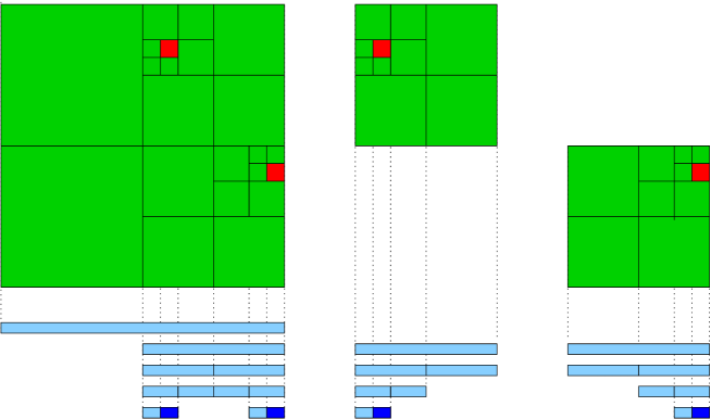
Figure 5: Block structures and corresponding column trees

Definition 11 (Column tree)

The column tree for $(t,r)\in\mathcal{T}_{\mathcal{I}\times\mathcal{K}}^{XY}$ is the minimal cluster tree $\mathcal{T}_{(t,r)}$

• with root $r$ and

• for every $r^{\prime}\in\mathcal{T}_{(t,r)}$ there is a $t^{\prime}\in\mathcal{T}_{\mathcal{I}}$ such that $(t^{\prime},r^{\prime})$ is a descendant of $(t,r)$ in the block tree $\mathcal{T}_{\mathcal{I}\times\mathcal{K}}^{XY}$,

• every $r^{\prime}\in\mathcal{T}_{(t,r)}$ is either a leaf or has the same children as it does in $\mathcal{T}_{\mathcal{K}}$.

The leaves of the column tree $\mathcal{T}_{(t,r)}$ are denoted by $\mathcal{L}_{(t,r)}$. A leaf $r^{\prime}\in\mathcal{L}_{(t,r)}$ is called inadmissible if a $t^{\prime}\in\mathcal{T}_{\mathcal{I}}$ with $(t^{\prime},r^{\prime})\in\mathcal{L}^{XY,-}_{\mathcal{I}\times\mathcal{K}}$ exists and admissible otherwise. The corresponding index sets $\{\hat{r}^{\prime}\ :\ r^{\prime}\in\mathcal{L}_{(t,r)}\}$ are a disjoint partition of the index set $\hat{r}$.

By construction $\mathcal{T}_{(t,r)}$ is a subtree of the cluster tree $\mathcal{T}_{\mathcal{K}}$.

The column tree $\mathcal{T}_{(t,r)}$ can be interpreted as an “orthogonal projection” of the subtree of $\mathcal{T}_{\mathcal{I}\times\mathcal{K}}^{XY}$ rooted at $(t,r)$ into its second component. Examples of block structures and the corresponding column trees can be seen in Figure 5.

Lemma 12 (Column representation)

Let $(t,r)\in\mathcal{T}_{\mathcal{I}\times\mathcal{K}}^{XY}$, and let $(t^{\prime},r^{\prime})\in\mathcal{L}^{XY,+}_{\mathcal{I}\times\mathcal{K}}$ be a descendant of $(t,r)$. Let $r^{*}\in\mathcal{L}_{(t,r)}$ be a descendant of $r^{\prime}$. There is a matrix $A\in\mathbb{R}^{\hat{t}^{\prime}\times k}$ with $G|_{\hat{t}\times\hat{r}^{*}}=AW_{r^{*}}^{*}$.

Proof 6.13.

This is a simple consequence of (2): due to $(t^{\prime},r^{\prime})\in\mathcal{L}^{XY,+}_{\mathcal{I}\times\mathcal{K}}$, we have

$$G|_{\hat{t}^{\prime}\times\hat{r}^{\prime}}=V_{t^{\prime}}S_{t^{\prime}r^{\prime}}W_{r^{\prime}}^{*},$$

and restricting to a child $r^{\prime\prime}\in\mathop{\operatorname{chil}}\nolimits(r^{\prime})$ leads to

$$G|_{\hat{t}^{\prime}\times\hat{r}^{\prime\prime}}=V_{t^{\prime}}S_{t^{\prime}r^{\prime}}F_{r^{\prime\prime}}^{*}W_{r^{\prime\prime}}^{*}$$

due to (2). We can proceed by induction until we reach the descendant $r^{*}$.

This lemma suggests how to perform condensation for subdivided matrices: for $(t,r)\in\mathcal{T}_{\mathcal{I}\times\mathcal{K}}^{XY}$, we enumerate the leaves $\mathcal{L}_{(t,r)}=\{r_{1},\ldots,r_{\ell}\}$ of the column tree $\mathcal{T}_{(t,r)}$ and see that Lemma 12 gives us matrices $A_{r_{1}},\ldots,A_{r_{\ell}}\in\mathbb{R}^{\hat{t}\times k}$ such that

$$G|_{\hat{t}\times\hat{s}}=\begin{pmatrix}A_{r_{1}}W_{r_{1}}^{*}&\ldots&A_{r_{\ell}}W_{r_{\ell}}^{*}\end{pmatrix}=\begin{pmatrix}A_{r_{1}}&\ldots A_{r_{\ell}}\end{pmatrix}\begin{pmatrix}W_{r_{1}}^{*}&&\\ &\ddots&\\ &&W_{r_{\ell}}^{*}\end{pmatrix},$$

where we can again drop the isometric left-most factor to get a matrix with only $\ell k$ columns.

In order to construct these condensed representations efficiently, we would like to use a recursive approach: first we construct representations for children of a block, then we merge them to get a representation for the parent. Figure 5 indicates a problem: different child blocks within the same column may have different column trees, and a common “super tree” has to be constructed to cover all of them.

Fortunately, we have again the nested structure (2) of the cluster basis $W$ at our disposal: if we have $r$ as a leaf in one column tree, while another column tree needs the children $\{r_{1}^{\prime},r_{2}^{\prime}\}=\mathop{\operatorname{chil}}\nolimits(r)$ of $r$, we simply use the transfer matrices $F_{r_{1}^{\prime}}$ and $F_{r_{2}^{\prime}}$ as in

$$A_{r}W_{r}^{*}=A_{r}\begin{pmatrix}W_{r_{1}^{\prime}}F_{r_{1}^{\prime}}\\ W_{r_{2}^{\prime}}F_{r_{2}^{\prime}}\end{pmatrix}^{*}=\begin{pmatrix}A_{r}F_{r_{1}^{\prime}}^{*}&A_{r}F_{r_{2}^{\prime}}^{*}\end{pmatrix}\begin{pmatrix}W_{r_{1}^{\prime}}^{*}&\\ &W_{r_{2}^{\prime}}^{*}\end{pmatrix}$$

to add representations for both children. We can apply this procedure to ensure that the representation for a column tree $\mathcal{T}_{(t^{\prime},r^{\prime})}$ of a sub-block $(t^{\prime},r^{\prime})$ matches a column tree $\mathcal{T}_{(t,r)}$ of its parent. The corresponding algorithm is given in Figure 6.

procedure match_column($r$, $\mathcal{T}$, $A$);
begin
	if $\mathop{\operatorname{chil}}\nolimits(r)\neq\emptyset$ then begin
		for $r^{\prime}\in\mathop{\operatorname{chil}}\nolimits(r)$ do
			match_column($r^{\prime}$, $\mathcal{T}$, $A$);
	end else if $\mathop{\operatorname{chil}}\nolimits_{\mathcal{T}}(r)\neq\emptyset$ then begin
		$\mathop{\operatorname{chil}}\nolimits(r)\leftarrow\mathop{\operatorname{chil}}\nolimits_{\mathcal{T}}(r)$;
		for $r^{\prime}\in\mathop{\operatorname{chil}}\nolimits(r)$ do begin
			$A_{r^{\prime}}\leftarrow A_{r}F_{r^{\prime}}^{*}$;
			match_column($r^{\prime}$, $\mathcal{T}$, $A$)
		end
	end else if $\mathop{\operatorname{adm}}\nolimits(r)$ and not $\mathop{\operatorname{adm}}\nolimits_{\mathcal{T}}(r)$ do begin
		$\mathop{\operatorname{adm}}\nolimits(r)\leftarrow\mathop{\operatorname{adm}}\nolimits_{\mathcal{T}}(r)$;
		$A_{r}\leftarrow A_{r}W_{r}^{*}$;
	end
end

Figure 6: Extending a column tree with root $r$ to match a given column tree $\mathcal{T}$. $\mathop{\operatorname{chil}}\nolimits(r)$ and $\mathop{\operatorname{adm}}\nolimits(r)$ denote the children of $r$ and its admissibility in its own column tree, $\mathop{\operatorname{chil}}\nolimits_{\mathcal{T}}(r)$ and $\mathop{\operatorname{adm}}\nolimits_{\mathcal{T}}(r)$ denote the children and the admissibility in the target tree $\mathcal{T}$.

Now we can return to the construction of the new cluster basis $Q$. As mentioned before, we proceed by recursion. On the way from the root towards the leaves, we accumulate total weight matrices $Z_{t}$ by computing thin Householder factorizations

$$P_{t}Z_{t}=\begin{pmatrix}Z_{t^{+}}E_{t}^{*}\\ S_{t,r_{1}}^{*}\\ \vdots\\ S_{t,r_{m}}\end{pmatrix},$$

where $t^{+}$ denotes the parent of $t$ if it exists (this submatrix vanishes in the root cluster) and $\{r_{1},\ldots,r_{m}\}=\mathop{\operatorname{row}}\nolimits_{XY}(t)$ are the column clusters of all admissible blocks with respect to the block tree $\mathcal{T}_{\mathcal{I}\times\mathcal{K}}^{XY}$, i.e.,

$$\mathop{\operatorname{row}}\nolimits_{XY}(t) :=\{r\in\mathcal{T}_{\mathcal{K}}\ :\ (t,r)\in\mathcal{L}^{XY,+}_{\mathcal{I}\times\mathcal{K}}\} \text{ for all }t\in\mathcal{T}_{\mathcal{I}}.$$

Using these weights, the entire part of $G_{t}$ or $\widehat{G}_{t}$ that is admissible in $\mathcal{T}_{\mathcal{I}\times\mathcal{K}}^{XY}$ can be condensed to $V_{t}Z_{t}^{*}$. This leaves us with the part that is inadmissible in $\mathcal{T}_{\mathcal{I}\times\mathcal{K}}^{XY}$, but admissible in $\mathcal{T}_{\mathcal{I}\times\mathcal{K}}$.

Leaf clusters.

Let $t\in\mathcal{L}_{\mathcal{I}}$ be a leaf of $\mathcal{T}_{\mathcal{I}}$. Since $t$ is a leaf, the only inadmissible blocks $(t,r)\in\mathcal{L}^{XY,-}_{\mathcal{I}\times\mathcal{K}}$ must correspond to nearfield matrices that are represented explicitly by our construction, i.e., $G|_{\hat{t}\times\hat{r}}$ is readily available to us.

Let $\{r_{1},\ldots,r_{m}\}$ denote all of these clusters, i.e., we have $(t,r_{i})\in\mathcal{L}^{XY,-}_{\mathcal{I}\times\mathcal{K}}$ for all $i\in[1:m]$ and an ancestor of each block is admissible in $\mathcal{T}_{\mathcal{I}\times\mathcal{K}}$. We use the condensed version $V_{t}Z_{t}^{*}$ of the admissible part in combination with the inadmissible parts to get

$$C_{t}:=\begin{pmatrix}V_{t}Z_{t}^{*}&G|_{\hat{t}\times\hat{r}_{1}}&\ldots&G|_{\hat{t}\times\hat{r}_{m}}\end{pmatrix}.$$ (20)

As mentioned before, the number of inadmissible blocks in $\mathcal{T}_{\mathcal{I}\times\mathcal{K}}^{XY}$ that are descendants of admissible blocks in $\mathcal{T}_{\mathcal{I}\times\mathcal{K}}$ is bounded, therefore $C_{t}$ has $\#\hat{t}$ rows and $\mathcal{O}(k)$ columns.

This makes it sufficiently small to compute the singular value decomposition of $C_{t}$ in $\mathcal{O}(k^{2}\#\hat{t})$ operations. We can use the singular values to choose an appropriate rank controlling the approximation error, and we can use the leading left singular vectors to set up the isometric matrix $Q_{t}$.

In preparation of the next steps, we also compute the basis-change matrix $R_{t}:=Q_{t}^{*}V_{t}$ and the auxiliary matrices

$$A_{t,r_{i}} =Q_{t}^{*}G|_{\hat{t}\times r_{i}} \text{ for all }i\in[1:m].$$

Non-leaf clusters.

Let now $t\in\mathcal{T}_{\mathcal{I}}\setminus\mathcal{L}_{\mathcal{I}}$ be a non-leaf cluster of $\mathcal{T}_{\mathcal{I}}$. For the sake of simplicity, we restrict out attention to the case $\mathop{\operatorname{chil}}\nolimits(t)=\{t_{1}^{\prime},t_{2}^{\prime}\}$. Since we are using recursion, $Q_{t_{1}^{\prime}}$ and $Q_{t_{2}^{\prime}}$ are already at our disposal, as are the basis changes $R_{t_{1}^{\prime}}$ and $R_{t_{2}^{\prime}}$ and the weights $A_{t_{1}^{\prime},r}$ and $A_{t_{2}^{\prime},r}$ for the inadmissible blocks connected to the children.

Our goal is to set up a condensed counterpart of the matrix

$$\widehat{G}_{t}:=\begin{pmatrix}Q_{t_{1}^{\prime}}^{*}G|_{\hat{t}_{1}^{\prime}\times\mathcal{R}_{t}}\\ Q_{t_{2}^{\prime}}^{*}G|_{\hat{t}_{2}^{\prime}\times\mathcal{R}_{t}}\end{pmatrix}.$$

Again, all the admissible parts are already represented by the weight matrix $Z_{t}$, and we can replace them all by

$$\widehat{V}_{t}Z_{t}^{*}\qquad\text{with}\qquad\widehat{V}_{t}:=\begin{pmatrix}Q_{t_{1}^{\prime}}^{*}V_{t_{1}^{\prime}}E_{t_{1}^{\prime}}\\ Q_{t_{2}^{\prime}}^{*}V_{t_{2}^{\prime}}E_{t_{2}^{\prime}}\end{pmatrix}=\begin{pmatrix}R_{t_{1}^{\prime}}E_{t_{1}^{\prime}}\\ R_{t_{2}^{\prime}}E_{t_{2}^{\prime}}\end{pmatrix}.$$

The inadmissible part is a little more challenging. We consider a cluster $r\in\mathcal{T}_{\mathcal{K}}$ with $(t,r)\in\mathcal{T}_{\mathcal{I}\times\mathcal{K}}^{XY}\setminus\mathcal{L}^{XY}_{\mathcal{I}\times\mathcal{K}}$, i.e., $(t,r)$ is subdivided. For the sake of simplicity, we assume $\mathop{\operatorname{chil}}\nolimits(r)=\{r_{1}^{\prime},r_{2}^{\prime}\}$ and have

$$G|_{\hat{t}\times\hat{r}}=\begin{pmatrix}G|_{\hat{t}_{1}^{\prime}\times\hat{r}_{1}^{\prime}}&G|_{\hat{t}_{1}^{\prime}\times\hat{r}_{2}^{\prime}}\\ G|_{\hat{t}_{2}^{\prime}\times\hat{r}_{1}^{\prime}}&G|_{\hat{t}_{2}^{\prime}\times\hat{r}_{2}^{\prime}}\end{pmatrix}.$$

We require only the projection into the ranges of $Q_{t_{1}^{\prime}}$ and $Q_{t_{2}^{\prime}}$, i.e.,

$$\begin{pmatrix}Q_{t_{1}^{\prime}}^{*}G|_{\hat{t}_{1}^{\prime}\times\hat{r}_{1}^{\prime}}&Q_{t_{1}^{\prime}}^{*}G|_{\hat{t}_{1}^{\prime}\times\hat{r}_{2}^{\prime}}\\ Q_{t_{2}^{\prime}}^{*}G|_{\hat{t}_{2}^{\prime}\times\hat{r}_{1}^{\prime}}&Q_{t_{2}^{\prime}}^{*}G|_{\hat{t}_{2}^{\prime}\times\hat{r}_{2}^{\prime}}\end{pmatrix}.$$

If one of these submatrices $Q_{t^{\prime}}^{*}G|_{\hat{t}^{\prime}\times\hat{r}^{\prime}}$ is again inadmissible, we have already seen it when treating the corresponding child $t^{\prime}$, and therefore $A_{t^{\prime},r^{\prime}}$ is already at our disposal.

Figure 7: Coarsening of a subdivided block: on the finest level (left) the submatrices are compressed individually. Stepping to a coarser level (right), the submatrices are merged by matching the column trees. Light green blocks are included in the parent’s weight $Z_{t}$.

If one of these submatrices $Q_{t^{\prime}}^{*}G|_{\hat{t}^{\prime}\times\hat{r}^{\prime}}$ is, on the other hand, admissible, we can use (1) and the basis-change matrix $R_{t^{\prime}}$ prepared previously to obtain

$$A_{t^{\prime},r^{\prime}}:=Q_{t^{\prime}}^{*}G|_{\hat{t}^{\prime}\times\hat{r}^{\prime}}=Q_{t^{\prime}}^{*}V_{t^{\prime}}S_{t^{\prime}r^{\prime}}W_{r^{\prime}}^{*}=R_{t^{\prime}}S_{t^{\prime}r^{\prime}}W_{r^{\prime}}^{*}.$$

Now that we have representations for all submatrices, we can use the function “match_column” of Figure 5 to ensure that they all share the same column tree $\mathcal{T}_{(t,r)}$ and combine them into the condensed matrix

$$\widehat{A}_{t,r} :=\begin{pmatrix}A_{t_{1}^{\prime},r_{1}}&\ldots&A_{t_{1}^{\prime},r_{\ell}}\\ A_{t_{2}^{\prime},r_{1}}&\ldots&A_{t_{2}^{\prime},r_{\ell}}\end{pmatrix}, \mathcal{L}_{(t,r)} =\{r_{1},\ldots,r_{\ell}\}.$$

Combining the admissible and inadmissible submatrices yields the condensed counterpart of $\widehat{G}_{t}$ in the form

$$\widehat{C}_{t}:=\begin{pmatrix}\widehat{V}_{t}Z_{t}^{*}&\widehat{A}_{t,r_{1}}&\ldots&\widehat{A}_{t,r_{m}}\end{pmatrix},$$ (21)

where $\{r_{1},\ldots,r_{m}\}$ again denotes all column clusters of blocks that are subdivided in $\mathcal{T}_{\mathcal{I}\times\mathcal{K}}^{XY}$ and have an admissible ancestor in $\mathcal{T}_{\mathcal{I}\times\mathcal{K}}$, i.e., $(t,r_{i})\in\mathcal{T}_{\mathcal{I}\times\mathcal{K}}^{XY}\setminus\mathcal{L}^{XY}_{\mathcal{I}\times\mathcal{K}}$ for all $i\in[1:m]$. As before, the number of inadmissible blocks in $\mathcal{T}_{\mathcal{I}\times\mathcal{K}}^{XY}$ as descendants of admissible blocks in $\mathcal{T}_{\mathcal{I}\times\mathcal{K}}$ is bounded, therefore the matrix $\widehat{C}_{t}$ has only $\mathcal{O}(k)$ columns and not more than $2k$ rows.

This makes it sufficiently small to compute the singular value decomposition in $\mathcal{O}(k^{3})$ operations, and we can again use the singular values to choose an appropriate rank controlling the approximation error and the leading left singular vectors to set up an isometric matrix $\widehat{Q}_{t}$.

We can split $\widehat{Q}_{t}$ into transfer matrices for $t_{1}^{\prime}$ and $t_{2}^{\prime}$ to get

$$Q_{t}:=U_{t}\widehat{Q}_{t},$$

i.e., the new cluster basis matrix $Q_{t}$ is expressed via transfer matrices as in (2).

We also compute the basis-change $R_{t}:=Q_{t}^{*}V_{t}=\widehat{Q}_{t}^{*}\widehat{V}_{t}$ and the auxiliary matrices

$$A_{t,r_{i}} =Q_{t}^{*}G|_{\hat{t}\times\hat{r}_{i}}=\widehat{Q}_{t}^{*}\widehat{A}_{t,r_{i}} \text{ for all }i\in[1:m]$$

in preparation for the next stage of the recursion. We can see that all of these operations take no more than $\mathcal{O}(k^{3})$ operations. The entire algorithm is summarized in Figure 8.

procedure build_basis($t$);
begin
	Compute $Z_{t}$ as in (19);
	if $\mathop{\operatorname{chil}}\nolimits(t)=\emptyset$ then begin
		Set up $C_{t}$ as in (20);
		Compute its singular value decomposition and choose a rank $k\in\mathbb{N}$;
		Build $Q_{t}$ from the first $k$ left singular vectors;
		$R_{t}\leftarrow Q_{t}^{*}V_{t}$;
		for $r\in\mathcal{T}_{\mathcal{K}}$ with $(t,r)\in\mathcal{L}^{XY,-}_{\mathcal{I}\times\mathcal{K}}$ do $A_{t,r}\leftarrow Q_{t}^{*}G|_{\hat{t}\times\hat{r}}$
	end
	else begin
		for $t^{\prime}\in\mathop{\operatorname{chil}}\nolimits(t)$ do build_basis($t^{\prime}$);
		Set up $\widehat{C}_{t}$ as in (21);
		Compute its singular value decomposition and choose a rank $k\in\mathbb{N}$;
		Build $\widehat{Q}_{t}$ from the first $k$ left singular vectors and set transfer matrices;
		$R_{t}\leftarrow\widehat{Q}_{t}^{*}\widehat{V}_{t}$;
		for $r\in\mathcal{T}_{\mathcal{K}}$ with $(t,r)\in\mathcal{T}_{\mathcal{I}\times\mathcal{K}}^{XY}\setminus\mathcal{L}^{XY}_{\mathcal{I}\times\mathcal{K}}$ do $A_{t,r}\leftarrow\widehat{Q}_{t}^{*}\widehat{A}_{t,r}$
	end
end

Figure 8: Recursive algorithm for constructing an adaptive row cluster basis using the coarse block tree $\mathcal{T}_{\mathcal{I}\times\mathcal{K}}$

Remark 6.14 (Complexity).

The basis construction algorithm has a complexity of $\mathcal{O}(nk^{2})$ if the following conditions are met:

• there are constants $c_{\text{lf}},C_{\text{lf}}$ with $c_{\text{lf}}k\leq\#\hat{t}\leq C_{\text{lf}}k$ for all leaf clusters $t\in\mathcal{T}_{\mathcal{I}}$,

• the block tree $\mathcal{T}_{\mathcal{I}\times\mathcal{K}}$ is sparse, i.e., there is a constant $C_{\text{sp}}$ with

  $$\#\{r\ :\ (t,r)\in\mathcal{T}_{\mathcal{I}\times\mathcal{K}}\} \leq C_{\text{sp}} \text{ for all }t\in\mathcal{T}_{\mathcal{I}},$$

• the fine block tree $\mathcal{T}_{\mathcal{I}\times\mathcal{K}}^{XY}$ is not too fine, i.e., there is a constant $C_{XY}$ with

  $$\#\{(t^{\prime},r^{\prime})\in\mathcal{T}_{\mathcal{I}\times\mathcal{K}}^{XY}\ :\ \hat{t}^{\prime}\times\hat{r}^{\prime}\subseteq\hat{t}\times\hat{r}\} \leq C_{XY} \text{ for all }(t,r)\in\mathcal{L}^{+}_{\mathcal{I}\times\mathcal{K}}.$$

The first condition ensures that the matrices $C_{t}$ and $\widehat{C}_{t}$ have only $\mathcal{O}(k)$ rows and that the cluster tree $\mathcal{T}_{\mathcal{I}}$ has only $\mathcal{O}(n/k)$ elements. The second and third conditions ensure that the matrices appearing in the construction of the weight matrices (19) have only $\mathcal{O}(k)$ columns. These conditions also ensure that the matrices $C_{t}$ and $\widehat{C}_{t}$ have only $\mathcal{O}(k)$ columns. Together, these three conditions guarantee that only $\mathcal{O}(k^{3})$ operations are required for every cluster, and since there are only $\mathcal{O}(n/k)$ clusters, we obtain $\mathcal{O}(nk^{2})$ operations in total.

7 Numerical experiments

We investigate the practical performance of the new algorithm by considering matrices appearing in the context of boundary element methods: the single-layer operator

$$\mathcal{V}[u](x) =\int_{\Gamma_{S}}\frac{1}{4\pi\|x-y\|}u(y)\,dy \text{ for all }x\in\Gamma_{S}$$

on the unit sphere $\Gamma_{S}:=\{x\in\mathbb{R}^{3}\ :\ \|x\|_{2}=1\}$, approximated on surface meshes constructed by starting with a double pyramid, splitting the faces regularly into triangles, and moving their vertices to the sphere, and the double-layer operator

$$\mathcal{K}[u](x) =\int_{\Gamma_{C}}\frac{\langle n(x),x-y\rangle}{4\pi\|x-y\|^{3}}u(y)\,dy \text{ for all }x\in\Gamma_{C}$$

on the surface of the cube $\Gamma_{C}:=\partial[-1,1]^{3}$, represented by surface meshes constructed by regularly splitting its six faces into triangles.

We discretize both operators by Galerkin’s method using piecewise constant basis functions on the triangular mesh. The resulting matrices are approximated using hybrid cross approximation [5] and converting the resulting hierarchical matrices into $\mathcal{H}^{2}$-matrices [4, Chapter 6.5]. For the single-layer operator on the unit sphere, we obtain matrices of dimensions between $2\,048$ and $2\,097\,152$, while we have dimensions between $3\,072$ and $3\,145\,728$ for the double-layer operator on the cube’s surface.

For the compression of the induced row and column basis, we use a block-relative accuracy of $10^{-4}$ as described in Section 5. For the re-compression into an $\mathcal{H}^{2}$-matrix with the final coarser block tree $\mathcal{T}_{\mathcal{I}\times\mathcal{K}}$, we use the same accuracy in combination with the block-relative error control strategy described in [4, Chapter 6.8].

$$\begin{array}[]{r|rrrr|rrrr}&\vrule\lx@intercol\hfil\text{Induced}\hfil\lx@intercol&\vrule\lx@intercol\hfil\text{Final}\hfil\lx@intercol\\ n&t_{\text{row}}&t_{\text{col}}&t_{\text{mat}}&\epsilon_{2}&t_{\text{row}}&t_{\text{col}}&t_{\text{mat}}&\epsilon_{2}\\ \hline\cr 2\,048&0.1&0.1&0.3&1.12_{-7}&0.4&0.2&0.0&1.12_{-5}\\ 4\,608&0.2&0.2&0.6&9.41_{-8}&1.3&0.7&0.1&5.91_{-6}\\ 8\,192&0.4&0.4&1.3&1.20_{-7}&2.6&1.5&0.2&4.87_{-6}\\ 18\,432&1.0&1.0&3.1&1.13_{-7}&6.6&3.8&0.5&4.93_{-6}\\ 32\,768&1.8&1.8&5.6&1.20_{-7}&12.1&7.1&0.8&4.79_{-6}\\ 73\,728&4.1&4.0&12.7&1.17_{-7}&28.6&16.3&1.8&4.98_{-6}\\ 131\,072&7.2&7.2&23.6&1.20_{-7}&53.3&29.8&3.3&5.07_{-6}\\ 294\,912&16.6&16.5&53.7&1.18_{-7}&120.5&68.0&7.9&4.77_{-6}\\ 524\,288&29.4&29.3&97.3&1.10_{-7}&215.2&121.7&13.4&4.87_{-6}\\ 1\,179\,648&65.8&65.7&218.1&1.00_{-7}&472.2&264.3&28.7&5.53_{-6}\\ 2\,097\,152&116.7&117.2&393.7&1.20_{-7}&875.9&487.4&53.5&4.76_{-6}\end{array}$$

Table 1: Run-times and relative spectral errors for the multiplication of the single-layer matrix

Table 1 lists the results of applying the new algorithm to multiply the single-layer matrix with itself. The “Induced” columns refer to the compression of the induced row and column cluster bases: $t_{\text{row}}$ gives the time in seconds for the row basis, $t_{\text{col}}$ the time for the column basis, and $t_{\text{mat}}$ the time for forming the $\mathcal{H}^{2}$-matrix using these bases and the full block tree $\mathcal{T}_{\mathcal{I}\times\mathcal{K}}^{XY}$. $\epsilon_{2}$ gives the relative spectral error, estimated by twenty steps of the power iteration. Here $1.12_{-7}$ is a short notation for $1.12\times 10^{-7}$.

The “Final” columns refer to the approximation of the product in the coarser block tree $\mathcal{T}_{\mathcal{I}\times\mathcal{K}}$. $t_{\text{row}}$ gives the time in seconds for the construction of the row basis for the coarse block tree, $t_{\text{col}}$ the time for the column basis, and $t_{\text{mat}}$ the time for forming the final $\mathcal{H}^{2}$-matrix with the coarse block tree $\mathcal{T}_{\mathcal{I}\times\mathcal{K}}$. $\epsilon_{2}$ is again the estimated relative spectral error.

These experiments were carried out on a single core of an AMD EPYC 7713 processor using the AOCL-BLIS library for linear algebra subroutines.

The time required to set up the cluster basis products $V_{X,s}^{*}W_{Y,s}$ and the total weights $Z_{t}$ for the first algorithm are not listed, since these operations’ run-times are negligible compared to the new algorithms.

We can see that the relative errors remain well below the prescribed bound of $10^{-4}$ and that the relative errors for the first phase are even smaller.

$$\begin{array}[]{r|rrrr|rrrr}&\vrule\lx@intercol\hfil\text{Induced}\hfil\lx@intercol&\vrule\lx@intercol\hfil\text{Final}\hfil\lx@intercol\\ n&t_{\text{row}}&t_{\text{col}}&t_{\text{mat}}&\epsilon_{2}&t_{\text{row}}&t_{\text{col}}&t_{\text{mat}}&\epsilon_{2}\\ \hline\cr 3\,072&0.2&0.2&0.4&9.13_{-7}&0.9&0.4&0.1&1.34_{-5}\\ 6\,912&0.6&0.4&1.2&1.57_{-6}&3.1&0.8&0.3&1.14_{-5}\\ 12\,288&1.2&0.7&2.2&1.89_{-6}&5.4&2.9&0.4&7.46_{-6}\\ 27\,648&2.9&1.7&5.7&2.90_{-6}&14.5&8.6&1.3&7.58_{-6}\\ 49\,152&5.3&3.0&10.1&3.43_{-6}&23.9&13.1&1.9&7.21_{-6}\\ 110\,592&12.1&7.0&23.9&4.52_{-6}&57.9&32.6&4.2&7.02_{-6}\\ 196\,608&21.4&12.3&41.9&4.95_{-6}&97.5&49.5&6.1&6.63_{-6}\\ 442\,368&47.9&27.7&97.3&5.72_{-6}&236.1&122.1&15.9&6.35_{-6}\\ 786\,432&86.5&47.4&169.0&6.15_{-6}&388.9&187.7&49.3&6.76_{-6}\\ 1\,769\,472&188.6&108.8&390.6&6.75_{-6}&926.2&454.2&72.2&7.79_{-6}\\ 3\,145\,728&338.7&190.7&673.0&7.12_{-6}&1562.5&765.6&109.9&7.79_{-6}\end{array}$$

Table 2: Run-times and relative spectral errors for the multiplication of the double-layer matrix

Table 2 shows the corresponding results for the double-layer matrix on the surface of the cube. We can again observe that the required accuracy is reliably provided.

Figure 9: Run-time for the adaptive $\mathcal{H}^{2}$-matrix multiplication per degree of freedom.

To see that the new algorithm indeed reaches the optimal linear complexity with respect to the matrix dimension $n$, we show the time divided by $n$ in Figure 9. We can see that the runtime per degree of freedom is bounded uniformly both for the single-layer and the double-layer matrix, i.e., we observe $\mathcal{O}(n)$ complexity.

In conclusion, we have found an algorithm that can approximate the product of two $\mathcal{H}^{2}$-matrices at a prescribed accuracy in linear, i.e., optimal complexity. In the first phase, the algorithm approximates the induced cluster bases for a refined intermediate block tree $\mathcal{T}_{\mathcal{I}\times\mathcal{K}}^{XY}$. In the second phase, an optimized representation for a prescribed block tree $\mathcal{T}_{\mathcal{I}\times\mathcal{K}}$ is constructed. Both phases can be performed with localized error control for all submatrices.

The fact that the matrix multiplication can indeed be performed in linear complexity leads us to hope that similar algorithms can be developed for important operations like the Cholesky or LU factorization, which would immediately give rise to efficient solvers for large systems of linear equations.

References

- [1] C. R. Anderson. An implementation of the fast multipole method without multipoles. SIAM J. Sci. Stat. Comp., 13:923–947, 1992.
- [2] M. Bebendorf and W. Hackbusch. Existence of -matrix approximants to the inverse FE-matrix of elliptic operators with -coefficients. Numer. Math., 95:1–28, 2003.
- [3] S. Börm. -matrix arithmetics in linear complexity. Computing, 77(1):1–28, 2006.
- [4] S. Börm. Efficient Numerical Methods for Non-local Operators: -Matrix Compression, Algorithms and Analysis, volume 14 of EMS Tracts in Mathematics. EMS, 2010.
- [5] S. Börm and L. Grasedyck. Hybrid cross approximation of integral operators. Numer. Math., 101:221–249, 2005.
- [6] S. Börm and W. Hackbusch. Data-sparse approximation by adaptive -matrices. Computing, 69:1–35, 2002.
- [7] S. Börm and W. Hackbusch. -matrix approximation of integral operators by interpolation. Appl. Numer. Math., 43:129–143, 2002.
- [8] S. Börm, M. Löhndorf, and J. M. Melenk. Approximation of integral operators by variable-order interpolation. Numer. Math., 99(4):605–643, 2005.
- [9] S. Börm and K. Reimer. Efficient arithmetic operations for rank-structured matrices based on hierarchical low-rank updates. Comp. Vis. Sci., 16(6):247–258, 2015.
- [10] S. Börm and S. A. Sauter. BEM with linear complexity for the classical boundary integral operators. Math. Comp., 74:1139–1177, 2005.
- [11] S. Chandrasekaran, M. Gu, and W. Lyons. A fast adaptive solver for hierarchically semiseparable representations. Calcolo, 42:171–185, 2005.
- [12] S. Chandrasekaran, M. Gu, and T. Pals. A fast ULV decomposition solver for hierarchically semiseparable representations. SIAM J. Matrix Anal. Appl., 28(3):603–622, 2006.
- [13] I. Gavrilyuk, W. Hackbusch, and B. N. Khoromskij. -matrix approximation for the operator exponential with applications. Numer. Math., 92:83–111, 2002.
- [14] I. Gavrilyuk, W. Hackbusch, and B. N. Khoromskij. Data-sparse approximation to operator-valued functions of elliptic operator. Mathematics of Computation, 73:1107–1138, 2004.
- [15] Z. Gimbutas and V. Rokhlin. A generalized fast multipole method for nonoscillatory kernels. SIAM J. Sci. Comput., 24(3):796–817, 2002.
- [16] L. Grasedyck. Existence of a low-rank or -matrix approximant to the solution of a Sylvester equation. Numer. Lin. Alg. Appl., 11:371–389, 2004.
- [17] L. Grasedyck and W. Hackbusch. Construction and arithmetics of -matrices. Computing, 70:295–334, 2003.
- [18] L. Grasedyck, W. Hackbusch, and B. N. Khoromskij. Solution of large scale algebraic matrix Riccati equations by use of hierarchical matrices. Computing, 70:121–165, 2003.
- [19] L. Grasedyck, R. Kriemann, and S. LeBorne. Domain decomposition based -LU preconditioning. Numer. Math., 112(4):565–600, 2009.
- [20] L. Greengard and V. Rokhlin. A fast algorithm for particle simulations. J. Comp. Phys., 73:325–348, 1987.
- [21] L. Greengard and V. Rokhlin. A new version of the fast multipole method for the Laplace equation in three dimensions. In Acta Numerica 1997, pages 229–269. Cambridge University Press, 1997.
- [22] W. Hackbusch. A sparse matrix arithmetic based on -matrices. Part I: Introduction to -matrices. Computing, 62(2):89–108, 1999.
- [23] W. Hackbusch. Hierarchical Matrices: Algorithms and Analysis. Springer, 2015.
- [24] W. Hackbusch, B. N. Khoromskij, and R. Kriemann. Hierarchical matrices based on a weak admissibility criterion. Computing, 73:207–243, 2004.
- [25] W. Hackbusch, B. N. Khoromskij, and S. A. Sauter. On -matrices. In H. Bungartz, R. Hoppe, and C. Zenger, editors, Lectures on Applied Mathematics, pages 9–29. Springer-Verlag, Berlin, 2000.
- [26] M. Ma and D. Jiao. Accuracy directly controlled fast direct solution of general -matrices and its application to solving electrodynamic volume integral equations. IEEE Trans. Microw. Theo. Tech., 66(1):35–48, 2018.
- [27] Q. Ma, S. Deshmukh, and R. Yokota. Scalable linear time dense direct solver for 3-D problems without trailing sub-matrix dependencies. Technical report, Tokyo Institut of Technology, 2022. arXiv 2208.10907.
- [28] V. Rokhlin. Rapid solution of integral equations of classical potential theory. J. Comp. Phys., 60:187–207, 1985.
- [29] V. Strassen. Gaussian elimination is not optimal. Numer. Math., 13(4):354–356, 1969.
- [30] J. Xia, S. Chandrasekaran, M. Gu, and X. S. Li. Fast algorithms for hierarchically semiseparable matrices. Numer. Lin. Alg. Appl., 2009. available at http://dx.doi.org/10.1002/nla.691.