Study of Enhanced MISC-Based Sparse Arrays with High uDOFs and Low Mutual Coupling

Abstract

In this letter, inspired by the maximum inter-element spacing (IES) constraint (MISC) criterion, an enhanced MISC-based (EMISC) sparse array (SA) with high uniform degrees-of-freedom (uDOFs) and low mutual-coupling (MC) is proposed, analyzed and discussed in detail. For the EMISC SA, an IES set is first determined by the maximum IES and number of elements. Then, the EMISC SA is composed of seven uniform linear sub-arrays (ULSAs) derived from an IES set. An analysis of the uDOFs and weight function shows that, the proposed EMISC SA outperforms the IMISC SA in terms of uDOF and MC. Simulation results show a significant advantage of the EMISC SA over other existing SAs.

I Introduction

Array signal processing techniques are gaining popularity in various applications, including radar [1], sonar [19, 20] etc. Traditional uniform linear arrays (ULAs) are usually utilized for beamforming [1],[2, 3, 4, 5, 6, 7, 8, 9, 10, 11, 12, 13, 14, 15, 16] and DOA estimation [4]. However, limited by the Rayleigh criterion, a $K$-element ULA can only resolve at most N-1 sources [24, 25]. $N$-1 sources can provide sufficient uniform degrees of freedom (uDOFs), allowing fewer sensors to achieve the spatial resolution of more targets [29]. Consequently, with the DCA concept applied to the existing SAs such as nested arrays (NAs) [30, 31] and coprime arrays (CAs) [43, 44], NAs can generate $O(\frac{K^{2}}{2})$ uDOFs for a $K$-element ULA but are vulnerable to mutual coupling (MC). In contrast, CAs have significantly fewer uDOFs than NAs but are more resistant to the MC effect.

Numerous SAs have been developed [11]-[14] through the prototype NAs and CAs. The early SAs are mostly aimed at how to increase the uDOFs. For few sensors, the minimum redundancy arrays (MRAs) is the most favorable choice due to the maximum uDOFs. NAs such as the improved NA (INA) [11], the CA having displaced-subarrays (CADiS) [12], the augmented NAs (ANA) [13], the two side-extended NA (TSENA) [14], and the flexible extended NA with multiple subarrays (f-ENAMS)[15] all demonstrate excellent enhancement on uDOFs. Nevertheless, the MC effect between the elements of small separation should not be neglected. Consequently, various SAs have been designed to reduce MC, such as the super NAs (SNAs) [15]-[18], the extended padded CAs (ePCAs) [19], and the improved coprime NA (ICNA) [20]. Moreover, another SA design method - the ULA fitting scheme composed of four base layers (UF-4BL) has been suggested with modest MC [21], [22]. Except for the conventional SA designs, an SA design based on the MISC criterion is presented and investigated [23]. The MISC-based SAs are developed via an IES set, jointly determined by the maximum IES and number of elements. For uDOFs, an improved MISC (IMISC) SA [24] is proposed with a much higher uDOF.

In this letter, compared with the IMISC SA, an enhanced MISC-based (EMISC) SA that further increases the uDOFs and reduces the MC effect is proposed. Then, relevant analysis is carried out from aspects of uDOF, MC and DOA estimation. Simulation results reflect a great advantage of the EMISC SA over other existing SAs.

Notation: Throughout this letter, lower-case (upper-case) characters represent vectors (matrices). Particularly, ${\rm{vec}}({\mathbf{I}}_{K})$ is the $K\times K$ identity matrix. The superscripts: $*$, $T$ and $H$ respectively represent the complex conjugate, transpose and conjugate transpose. The operators: $E[\cdot]$ denotes the statistical expectation operator; ${\rm{vec}}(\cdot)$ denotes the vectorization operator; ${\rm{diag}}(\cdot)$ denotes the diagonalization operator; ${\rm{card}}\{\cdot\}$ denotes the element number of a set and $\lfloor\cdot\rfloor$ denotes the floor operator. The symbols: $\odot$ is the Khatri-Rao product; $\lvert\cdot\rvert$ is the absolute value; $\|\cdot\|_{F}$ is the Frobenius norm, $\%$ is the remainder and $\cup$ denotes the union operator.

II Coarray Concept and Mutual Coupling

II-A DCA Model

First, let us choose a $K$-element nonuniform linear array, whose element positions are given by $p_{i}d$, where $p_{i}\in\mathbb{P}$. $d={{\lambda}/2}$ denotes the minimum inter-element spacing, with ${\lambda}$ being the wavelength of the incident wave.

$$\mathbb{P}=\left\{{{p_{0}},p_{1},p_{2},\dots,p_{K-1}}\right\},$$ (1)

Assume that $N$ far-field, uncorrelated narrowband sources arrive at the array from different bearings $\left\{\theta_{i},i=1,\cdots,N\right\}$ corresponding to the powers $\left\{\rho^{2}_{i},i=1,\cdots,N\right\}$.

Then, the received signal can be modeled as

$${\mathbf{x}}={\mathbf{A}}{\mathbf{s}}+{\mathbf{n}},$$ (2)

where $\mathbf{s}\triangleq\left[\mathbf{s}_{1},\cdots,\mathbf{s}_{N}\right]^{T}$ denotes the incident sources, and ${\mathbf{n}}$ is the additive Gaussian white noise, uncorrelated with the sources. Besides, $\mathbf{A}\triangleq\left[\mathbf{a}_{\theta_{1}},\cdots,\mathbf{a}_{\theta_{N}}\right]$ is the $K\times N$ array manifold matrix, where the corresponding steering vector $\mathbf{a}_{{\theta}_{i}}=\left[e^{j\frac{2\pi}{\lambda}p_{0}d\sin({\theta}_{i})},\cdots,e^{j\frac{2\pi}{\lambda}p_{K-1}d\sin({\theta}_{i})}\right]^{T}$, ${\theta}_{i}$ is the bearing of the $i^{th}$ source.

Next, the covariance matrix (CM) of (2) is given by

$${\mathbf{R}_{\mathbf{x}}}\triangleq E[\mathbf{x}{\mathbf{x}^{H}}]=\mathbf{A}\mathbf{R}_{\mathbf{s}}{\mathbf{A}^{H}}+\rho_{n}^{2}\mathbf{I}_{K},$$ (3)

where $\mathbf{R}_{\mathbf{s}}$ is the CM of the received signal and $\rho^{2}_{n}$ is the noise power.

Finally, (3) is vectorized as (4), expressed as

$${\mathbf{y}}\triangleq{\rm{vec}}({\mathbf{R}_{\mathbf{x}}})=({\mathbf{A}}^{*}\odot{\mathbf{A}}){\mathbf{h}}+\rho_{n}^{2}{\mathbf{1}}_{k},$$ (4)

where $\mathbf{1}_{k}={\rm{vec}}({\mathbf{I}}_{K})$, and ${\mathbf{h}}=\left[\rho^{2}_{1},\cdots,\rho^{2}_{N}\right]^{T}$ is the received signal of the DCA, defined by (5) [30]

$$\mathbb{D}=\left\{{{p_{a}-p_{b}},a,b=0,1,\cdots K-1}\right\}.$$ (5)

II-B MC effect

Considering the MC effect in practical application, (6) is obtained by interpolating the MC matrix $\mathbf{U}$ into (2).

$${\mathbf{x}}={\mathbf{U}}{\mathbf{A}}{\mathbf{s}}+{\mathbf{n}},$$ (6)

where, $\mathbf{U}$ is a $K\times K$ $G$-banded identity matrix [23]-[24].

$${\mathbf{U}}_{b,c}=\left\{{\begin{array}[]{*{20}{l}}u_{|p_{b}-p_{c}|},&|p_{b}-p_{c}|\leq G,\\ 0,&{\rm{elsewhere}},\end{array}}\right.$$ (7)

where, $p_{b},p_{c}\in\mathbb{P}$, $v=|p_{b}-p_{c}|\in[0,G]$, and $u_{v}$ denotes an arbitrary element of $\mathbb{U}$ that is expressed as

$$\left\{{\begin{array}[]{*{20}{l}}u_{0}=1\textgreater|u_{1}|\textgreater|u_{2}|\textgreater\cdots\textgreater|u_{G}|,\\ |u_{i}/u_{j}|=j/i,\quad\hskip 3.00003pt\ i,j\in[1,G].\end{array}}\right.$$ (8)

The MC effect is usually measured by the coupling leakage (CL), given by

$$M=\frac{||{\mathbf{U}}-{\rm{diag}}({\mathbf{U}})||_{F}}{||{\mathbf{U}}||_{F}}.$$ (9)

The weight function $w(l)$, which outputs the number of element pairs whose IES is l, is defined as

$$w(l)={\rm{card}}\{(p_{i},p_{j})|p_{i}-p_{j}=l;p_{i},p_{j}\in\mathbb{P}\}.$$ (10)

By the analysis above, there is a close relationship between MC and the weight function. Besides, the first three weight values $w(i),i=1,2,3$ jointly dominate the MC matrix.

III Proposed EMISC SA

Considering that the IMISC SA is composed of six ULSAs [24], another ULSA with an IES of 3 is added to reduce the MC. Then, all ULSAs are reasonably rearranged and optimized to enable $w(1)$ equal to one. Thereby, compared with the IMISC SA, we propose an enhanced MISC-based (EMISC) SA, which achieves higher uDOFs and lower MC, and has a closed-form expression of IES set, position set, and uDOF.

III-A SA Configuration

Based on the MISC criterion, the EMISC SA configuration is schemed by an IES set, which depends on the maximum IES and the number of elements. Then, the closed-form expression of the IES set $\mathbb{S}_{\text{EMISC}}$ is provided as

$$\mathbb{S}_{\text{EMISC}}=\left\{\begin{array}[]{l}3,\underbrace{2,...,2}_{\frac{L}{4}-1},\underbrace{L/2+1,...,L/2+1}_{\frac{L}{4}-1},\\ \underbrace{L,...,L}_{K-L},\underbrace{L/2-1,...,L/2-1}_{\frac{L}{4}-2},\\ \frac{L}{2}-2,1,3,\underbrace{2,...,2}_{\frac{L}{4}-2},\end{array}\right\},$$ (11)

where $K$ is the number of elements, $L$ is the maximum IES and

$$L=4\lfloor\frac{K-4}{6}\rfloor+4,K\geq 10,\\$$ (12)

According to (11), the position set is given by

$$\mathbb{P}_{\text{EMISC}}=$$ (13)

$$\left\{\begin{array}[]{l}\underbrace{0,3}_{{\text{ULA 1, IES=3}}},\underbrace{5,...,\frac{L}{2}+1}_{{\text{ULA 2, IES=2}}},\underbrace{\frac{L}{2}+3,...,\frac{{{L^{2}}}}{8}-\frac{L}{4}+1}_{{\text{ULA 3, IES=}}\frac{L}{2}+1},\\ \underbrace{\frac{{{L^{2}}}}{8}+\frac{{L}}{4}+2,...,-\frac{{7{L^{2}}}}{8}+(K-\frac{3}{4})L+2}_{{\text{ULA 4, IES=}}L},\\ \underbrace{-\frac{{7{L^{2}}}}{8}+(K+\frac{1}{4})L+2,...,-\frac{{3{L^{2}}}}{4}+(K-1)L+4}_{{\text{ULA 5, IES=}}\frac{L}{2}-1},\\ \underbrace{-\frac{{3{L^{2}}}}{4}+(K-\frac{1}{2})L+2,-\frac{{3{L^{2}}}}{4}+(K-\frac{1}{2})L+3}_{{\text{ULA 6, IES=1}}},\\ \underbrace{-\frac{{3{L^{2}}}}{4}+(K-\frac{1}{2})L+6,...,-\frac{{3{L^{2}}}}{4}+KL+2}_{{\text{ULA 7, IES=2}}},\\ \end{array}\right\}$$

It is noted that the EMISC SA is made up of seven ULSAs. Fig. 1 represents a specific EMISC SA configuration with an element number $K$ = 10 and the maximum IES $L$ = 8, where sub-i ($i=1,...,7$) denotes the i-th ULSA, respectively.

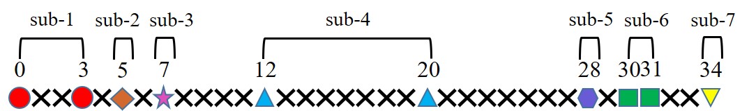
Figure 1: The EMISC SA configuration with $K=10$ and $L=8$.

III-B Consecutive part in the DCA

Considering the symmetric property of the DCA, we just need to prove $\mathbb{C}_{\text{EMISC}}^{+}\subset\mathbb{D}_{\text{EMISC}}^{+}$, where $\mathbb{C}_{\text{EMISC}}^{+}$ and $\mathbb{D}_{\text{EMISC}}^{+}$ represent the positive part of $\mathbb{C}_{\text{EMISC}}$ and $\mathbb{D}_{\text{EMISC}}$, respectively. (14) gives the position sets of any two ULSAs.

$$\mathbb{P}_{\text{ULSA}_{m}} =\{p_{m}(x),x=1,\dots,K_{m}\},$$ (14)

$$\mathbb{P}_{\text{ULSA}_{n}} =\{p_{n}(x),x=1,\dots,K_{n}\}.$$

where $K_{m}$ and $K_{n}$ separately denotes the element number of ULSA-$m$ and ULSA-$n$, and the DCA $\mathbb{D}_{m,n}$ between ULSA-$m$ and ULSA-$n$ is defined as

$$\mathbb{D}_{m,n}=\{p_{n}(y)-p_{m}(x)\,x=1,\dots,K_{m}\,y=1,\dots,K_{n}\}.$$ (15)

where, $\mathbb{D}_{m,m}=\{p_{m}(x)-p_{m}(1),x=1,\dots,K_{m}\}$.

Considering the fact that the proposed EMISC SA is composed of seven ULSAs, then, the positive part $\mathbb{D}_{\text{EMISC}}^{+}$ in the DCA $\mathbb{D}_{\text{EMISC}}$ of the proposed EMISC SA is expressed as

$$\mathbb{D}_{\text{EMISC}}^{+}=\bigcup_{m=1}^{7}\mathbb{D}_{\text{m,n}}^{+},n=m,m+1,\dots,7,$$ (16)

where $\mathbb{D}_{\text{m,n}}^{+}$ is the positive part of $\mathbb{D}_{m,n}$. $\mathbb{C}_{\text{EMISC}}^{+}\subset\mathbb{D}_{\text{EMISC}}^{+}$ is derived by finding DCAs to make up the consecutive part $[0,-\frac{{3{L^{2}}}}{4}+(K-\frac{1}{2})L+3]$.

$\mathbb{D}_{1,1}\cup\mathbb{D}_{1,2}\cup\mathbb{D}_{1,3}\cup\mathbb{D}_{2,3}\cup\mathbb{D}_{5,6}\cup\mathbb{D}_{5,7}\cup\mathbb{D}_{6,6}\cup\mathbb{D}_{6,7}$ generates a consecutive range $\mathbb{R}_{1}$, as shown in (17).

$$[0,\frac{L^{2}}{8}-\frac{L}{4}+1].$$ (17)

$\mathbb{D}_{1,4}\cup\mathbb{D}_{2,4}\cup\mathbb{D}_{3,4}\cup\mathbb{D}_{4,4}\cup\mathbb{D}_{4,5}\cup\mathbb{D}_{4,6}\cup\mathbb{D}_{4,7}$ generates a consecutive range $\mathbb{R}_{2}$, as seen in (18).

$$[\frac{L^{2}}{8}-\frac{L}{4}+1,-\frac{7L^{2}}{8}+(K-\frac{1}{4})L].$$ (18)

$\mathbb{D}_{1,6}\cup\mathbb{D}_{2,5}\cup\mathbb{D}_{2,6}\cup\mathbb{D}_{3,5}\cup\mathbb{D}_{3,6}\cup\mathbb{D}_{3,7}$ generates a consecutive range $\mathbb{R}_{3}$, as given in (19).

$$[-\frac{7L^{2}}{8}+(K-\frac{1}{4})L+1,-\frac{{3{L^{2}}}}{4}+(K-\frac{1}{2})L+3].$$ (19)

Finally, it is proved that $\mathbb{C}_{\text{EMISC}}^{+}=\mathbb{R}_{1}\cup\mathbb{R}_{2}\cup\mathbb{R}_{3}\subset\mathbb{D}_{\text{EMISC}}^{+}$. Moreover, $\mathbb{C}_{\text{EMISC}}^{+}$ is the maximum consecutive part of $\mathbb{D}_{\text{EMISC}}^{+}$, owing to a hole at the position of $-\frac{{3{L^{2}}}}{4}+(K-\frac{1}{2})L+4$.

The expressions of self-DCAs among ULSAs in the proposed EMISC SA are provided as

$$\mathbb{D}_{\text{1,1}}={\Big{\{}0,3\Big{\}},}$$

$$\mathbb{D}_{\text{2,2}}={\Big{\{}0,2,\dots,\frac{L}{2}-4\Big{\}},}$$

$$\mathbb{D}_{\text{3,3}}={\Big{\{}0,1,\dots,\frac{L}{4}-2)(\frac{L}{2}+1)\Big{\}},}$$

$$\mathbb{D}_{\text{4,4}}={\Big{\{}(0,1,\dots,K-L-1)L\Big{\}},}$$

$$\mathbb{D}_{\text{5,5}}={\Big{\{}(0,1,\dots,\frac{L}{4}-2)(\frac{L}{2}-1)\Big{\}},}$$

$$\mathbb{D}_{\text{6,6}}={\Big{\{}0,1\Big{\}},}$$

$$\mathbb{D}_{\text{7,7}}={\Big{\{}0,2,\dots,\frac{L}{2}-4\Big{\}}.}$$

The expressions of cross-DCAs are provided as

$$\mathbb{D}_{\text{1,2}}=\Big{\{}2+i+j\Big{\}},$$

$$\mathbb{D}_{\text{1,3}}=\Big{\{}\frac{L}{2}+i+j\Big{\}},$$

$$\mathbb{D}_{\text{1,4}}=\Big{\{}\frac{L^{2}}{8}+\frac{L}{4}-1+i+j\Big{\}},$$

$$\mathbb{D}_{\text{1,5}}=\Big{\{}-\frac{7L^{2}}{8}+(K+\frac{1}{4})L-1+i+j\Big{\}},$$

$$\mathbb{D}_{\text{1,6}}=\Big{\{}-\frac{3L^{2}}{4}+(K-\frac{1}{2})L-1+i+j\Big{\}},$$

$$\mathbb{D}_{\text{1,7}}=\Big{\{}-\frac{3L^{2}}{4}+(K-\frac{1}{2})L+3+i+j\Big{\}},$$

$$\mathbb{D}_{\text{2,3}}=\Big{\{}2+i+j\Big{\}},$$

$$\mathbb{D}_{\text{2,4}}=\Big{\{}\frac{L^{2}}{8}-\frac{L}{4}+1+i+j\Big{\}},$$

$$\mathbb{D}_{\text{2,5}}=\Big{\{}-\frac{7L^{2}}{8}+(K-\frac{1}{4})L+1+i+j\Big{\}},$$

$$\mathbb{D}_{\text{2,6}}=\Big{\{}-\frac{3L^{2}}{4}+(K-1)L+1+i+j\Big{\}},$$

$$\mathbb{D}_{\text{2,7}}=\Big{\{}-\frac{3L^{2}}{4}+(K-1)L+5+i+j\Big{\}},$$

$$\mathbb{D}_{\text{3,4}}=\Big{\{}\frac{L}{2}+1+i+j\Big{\}},$$

$$\mathbb{D}_{\text{3,5}}=\Big{\{}-L^{2}+(K+\frac{1}{2})L+1+i+j\Big{\}},$$

$$\mathbb{D}_{\text{3,6}}=\Big{\{}-\frac{7L^{2}}{8}+(K-\frac{1}{4})L+1+i+j\Big{\}},$$

$$\mathbb{D}_{\text{3,7}}=\Big{\{}-\frac{7L^{2}}{8}+(K-\frac{1}{4})L+5+i+j\Big{\}},$$

$$\mathbb{D}_{\text{4,5}}=\Big{\{}L+i+j\Big{\}},$$

$$\mathbb{D}_{\text{4,6}}=\Big{\{}\frac{L^{2}}{8}+\frac{L}{4}+i+j\Big{\}},$$

$$\mathbb{D}_{\text{4,7}}=\Big{\{}\frac{L^{2}}{8}+\frac{L}{4}+4+i+j\Big{\}},$$

$$\mathbb{D}_{\text{5,6}}=\Big{\{}\frac{L}{2}-2+i+j\Big{\}},$$

$$\mathbb{D}_{\text{5,7}}=\Big{\{}\frac{L}{2}+2+i+j\Big{\}},$$

$$\mathbb{D}_{\text{6,7}}=\Big{\{}3+i+j\Big{\}}.$$

where,

$$\mathbb{D}_{\text{\it}{m,n}}\hskip 5.0pt(m\leq n,\hskip 5.0ptm=1,2,\dots,6,7;\hskip 5.0ptn=1,2,\dots,6,7.)$$

$$1)\quad m=1,\quad i=(0,3);$$

$$2)\quad m=2,\quad i=(0,2,\dots,\frac{L}{2}-4);$$

$$3)\quad m=3,\quad i=(0,1,\dots,\frac{L}{4}-2)(\frac{L}{2}+1);$$

$$4)\quad m=4,\quad i=(0,1,\dots,K-L-1)(L);$$

$$5)\quad m=5,\quad i=(0,1,\dots,\frac{L}{4}-2)(\frac{L}{2}-1);$$

$$6)\quad m=6,\quad i=(0,1);$$

$$7)\quad m=7,\quad i=(0,2,\dots,\frac{L}{2}-4).$$

Likewise, the variables $$n j m i$$ and are presented like and above.

III-C uDOF Derivation

Based on the proof in Section III. B, (20) gives the expression of the consecutive part $\mathbb{C}_{\text{EMISC}}$

$$\mathbb{C}_{\text{EMISC}}=[\frac{{3{L^{2}}}}{4}-(K-\frac{1}{2})L-3,-\frac{{3{L^{2}}}}{4}+(K-\frac{1}{2})L+3].$$ (20)

Then, the maximum uDOF of EMISC SA is provided by

$${\text{uDOF}}_{\text{EMISC}}=-\frac{{3{L^{2}}}}{2}+(2K-1)L+7.$$ (21)

Interpolating (12) into (21), ${\text{uDOF}}_{\text{EMISC}}$ is given as

$${{\text{uDOF}}_{\text{EMISC}}=\left\{{\begin{array}[]{*{20}{l}}\frac{{{\rm{2}}{K^{2}}}}{3}-\frac{{2K}}{3}+3,&K\%6=3,4\\ \frac{{{\rm{2}}{K^{2}}}}{3}-\frac{{2K}}{3}+\frac{17}{3},&K\%6=2,5,\\ \frac{{{\rm{2}}{K^{2}}}}{3}-\frac{{2K}}{3}+7,&K\%6=0,1\end{array}}\right.}$$ (22)

Comparatively, the uDOF of the IMISC SA is presented as

$${{\text{uDOF}}_{\text{IMISC}}=\left\{{\begin{array}[]{*{20}{l}}\frac{{{\rm{2}}{K^{2}}}}{3}-\frac{{2K}}{3}-1,&K\%6=3,4\\ \frac{{{\rm{2}}{K^{2}}}}{3}-\frac{{2K}}{3}+\frac{5}{3},&K\%6=2,5.\\ \frac{{{\rm{2}}{K^{2}}}}{3}-\frac{{2K}}{3}+3,&K\%6=0,1\end{array}}\right.}$$ (23)

(22) and (23) show that both EMISC and IMISC SAs are able to utilize $K$ elements to generate $O(\frac{2K^{2}}{3})$ uDOFs, higher than most existing SAs. Meanwhile, it’s found that the EMISC SA has four more uDOFs than the IMISC SA.

III-D Weight Function

Considering that the first three weight values $w(i)(i=1,2,3)$ jointly dominate the MC matrix. Thus, $w(i)(i=1,2,3)$ of the EMISC SA are provided by

$$w(1)=1,~{}w(2)=2,\quad\quad\quad\hskip 8.00003pt~{}w(3)=2, 10\leq K<16,$$ (24)

$$w(1)=1,~{}w(2)=2\lfloor\frac{K-4}{6}\rfloor,~{}w(3)=2, K\geq 16.$$

Likewise, $w(i)(i=1,2,3)$ of the IMISC SA are listed as

$$w(1)=2,~{}w(2)=5,\quad\quad\quad\hskip 6.99997pt~{}w(3)=2, 10\leq K<16,$$ (25)

$$w(1)=2,~{}w(2)=2\lfloor\frac{K+2}{6}\rfloor,~{}w(3)=1, K\geq 16.$$

(24) and (25) confirm that the EMISC SA has a much lower MC than the IMISC SA. Thus, the CL of MISC-based SAs ranks in such an order: EMISC$<$IMISC$<$MISC.

IV Numerical Simulations

The proposed EMISC SA is compared with ANAI-2 [13], TSENA [14], f-ENAMS-II [15], SNAs [16]-[18], ePCA [19], ICNA [20], UF-4BL [21], [22], MISC [23] and IMISC [24] SAs. Besides, DOA estimation performance is analyzed via the spatial-smoothing MUSIC (SS-MUSIC), utilizing 1000 snapshots of data, and a coupling parameter  $u_{k}=u_{1}e^{-j(k-1)\pi/8}/k,\,k=2,\dots,100$.

IV-A uDOF and CL

The EMISC SA is compared with other existing SAs in Fig. 2, from aspects of uDOF and CL.

(a) uDOF.

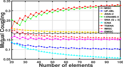
(b) CL.

Figure 2: uDOF and CL versus number of elements.

Fig. 2(a) provides the curves that illustrate the effect of the element number on the uDOF. It is noted that the EMISC SA behaves best among all SAs. As the number of elements increases, the advantages of the EMISC SA gradually become prominent, owing to the $O(2K^{2}/3)$ uDOF of the EMISC SA, superior to the maximum uDOF $O(4K^{2}/7)$ of other existing SAs.

Fig. 2(b) reflects how the number of element affects the CL. The CL of the EMISC SA is lower than that of the IMISC SA, but still higher than that of ICNA and UF-4BL. In sum, Fig. 2 confirms that the EMISC SA outperforms other existing SAs, in terms of uDOF and CL.

IV-B RMSE versus SNR and $|u_{1}|$

Here, through 500 Monte Carlo experiments, Fig. 3 assesses the DOA estimation performance by RMSE versus SNR and $|u_{1}|$. 48 sources uniformly distributed among $[-60^{o}60^{o}]$ are received by 36-element SAs. Under a fixed coupling parameter  $u_{1}=0.3e^{j\pi/3}$, the RMSE versus SNR is illustrated in Fig. 3(a). For a fixed SNR=0 dB, the RMSE versus $|u_{1}|$ ranging from 0 to 0.5 is demonstrated in Fig. 3(b).

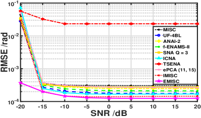
(a) RMSE versus SNR.

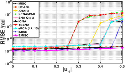
(b) RMSE versus $|u_{1}|$.

Figure 3: RMSE performance versus SNR and $|u_{1}|$.

To sum up, compared to all mentioned SAs above, Fig. 3 verifies that the proposed EMISC SA possesses the lowest RMSE, from aspects of SNR and $|u_{1}|$.

V Data Processing

Here, DOA estimation performance of the proposed EMISC SA is verified by real data collected in an underwater target detection trial on Sep. 24-25th, 2020. A 15-element receiver SA was deployed at the seabed. The observed angle is measured from the broadside of the receiver SA, within a range of [-90°,90°]. Occasionally, there appeared some operating fishing boats. The received data was composed of ninety 20s-packages and processed at a frequency band of [50Hz,120Hz].

Fig. 4 gives the bearing-time records (BTRs). It is observed that there exists a weak target (-3°) and two neighboring targets (63°, 68°). The weak target gets detected in the BTRs of all SAs in Fig. 4. Due to the variance of uDOF, two neighboring targets cannot be distinguished in Figs. 4(a), (b) and (c), while it works in Figs. 4(d), (e) and (f). Compared to Figs. 4(e) and (f), the bearing resolution of two neighboring targets appears blurry in Fig. 4(d). Considering no MC in the underwater acoustic arrays, the EMISC SA basically performs as well as the IMISC SA, owing to the approximately same uDOFs.

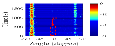
(a) ANAI2.

(b) UF-4BL.

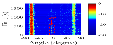
(c) ICNA.

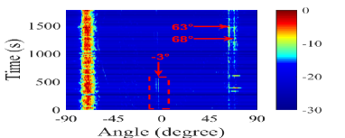
(d) MISC.

(e) IMISC.

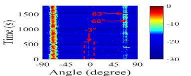
(f) EMISC.

Figure 4: The bearing-time records (BTRs).

VI Conclusion

In this letter, an enhanced MISC-based (EMISC) sparse array (SA) with high uDOFs and low MC effect is proposed. The EMISC SA is designed via an IES set, determined by the maximum IES and the number of element. The uDOF and weight-function of the EMISC SA are derived in theory. Compared to the IMISC SA, the EMISC SA further increases the uDOFs and reduces the MC. For DOA estimation, the EMISC SA has a much lower RMSE than other existing SAs. Finally, the EMISC SA is verified by real data.

References

• [1] C. FLe, Principles of Radar and Sonar Signal Processing., Artech House, 2002.
• [2] L. Wang, R. C. de Lamare and M. Yukawa, ”Adaptive Reduced-Rank Constrained Constant Modulus Algorithms Based on Joint Iterative Optimization of Filters for Beamforming,” in IEEE Transactions on Signal Processing, vol. 58, no. 6, pp. 2983-2997, June 2010.
• [3] Wang, L.; de Lamare, R.C.: ’Constrained adaptive filtering algorithms based on conjugate gradient techniques for beamforming’, IET Signal Processing, 2010, 4, (6), p. 686-697.
• [4] Wang, L.; de Lamare, R.C.: ’Set-membership constrained conjugate gradient adaptive algorithm for beamforming’, IET Signal Processing, 2012, 6, (8), p. 789-797.
• [5] R. Fa and R. C. De Lamare, ”Reduced-Rank STAP Algorithms using Joint Iterative Optimization of Filters,” in IEEE Transactions on Aerospace and Electronic Systems, vol. 47, no. 3, pp. 1668-1684, July 2011
• [6] L. Wang and R. C. DeLamare, ”Low-Complexity Constrained Adaptive Reduced-Rank Beamforming Algorithms,” in IEEE Transactions on Aerospace and Electronic Systems, vol. 49, no. 4, pp. 2114-2128, October 2013
• [7] Landau, L., de Lamare, R.C. and Haardt, M. (2014), Robust adaptive beamforming algorithms using the constrained constant modulus criterion. IET Signal Process., 8: 447-457.
• [8] N. Song, R. C. de Lamare, M. Haardt and M. Wolf, ”Adaptive Widely Linear Reduced-Rank Interference Suppression Based on the Multistage Wiener Filter,” in IEEE Transactions on Signal Processing, vol. 60, no. 8, pp. 4003-4016, Aug. 2012.
• [9] N. Song, W. U. Alokozai, R. C. de Lamare and M. Haardt, ”Adaptive Widely Linear Reduced-Rank Beamforming Based on Joint Iterative Optimization,” in IEEE Signal Processing Letters, vol. 21, no. 3, pp. 265-269, March 2014.
• [10] Yang, Z.; de Lamare, R.C.; Li, X.: ’Sparsity-aware space–time adaptive processing algorithms with L1-norm regularisation for airborne radar’, IET Signal Processing, 2012, 6, (5), p. 413-423.
• [11] S. D. Somasundaram, N. H. Parsons, P. Li and R. C. de Lamare, ”Reduced-dimension robust capon beamforming using Krylov-subspace techniques,” in IEEE Transactions on Aerospace and Electronic Systems, vol. 51, no. 1, pp. 270-289, January 2015.
• [12] X. Wu, Y. Cai, M. Zhao, R. C. de Lamare and B. Champagne, ”Adaptive Widely Linear Constrained Constant Modulus Reduced-Rank Beamforming,” in IEEE Transactions on Aerospace and Electronic Systems, vol. 53, no. 1, pp. 477-492, Feb. 2017.
• [13] Y. Zhaocheng, R. C. de Lamare and W. Liu, ”Sparsity-Based STAP Using Alternating Direction Method With Gain/Phase Errors,” in IEEE Transactions on Aerospace and Electronic Systems, vol. 53, no. 6, pp. 2756-2768, Dec. 2017.
• [14] H. Ruan and R. C. de Lamare, ”Robust Adaptive Beamforming Using a Low-Complexity Shrinkage-Based Mismatch Estimation Algorithm,” in IEEE Signal Processing Letters, vol. 21, no. 1, pp. 60-64, Jan. 2014.
• [15] H. Ruan and R. C. de Lamare, ”Robust Adaptive Beamforming Based on Low-Rank and Cross-Correlation Techniques,” in IEEE Transactions on Signal Processing, vol. 64, no. 15, pp. 3919-3932, 1 Aug.1, 2016.
• [16] H. Ruan and R. C. de Lamare, ”Distributed Robust Beamforming Based on Low-Rank and Cross-Correlation Techniques: Design and Analysis,” in IEEE Transactions on Signal Processing, vol. 67, no. 24, pp. 6411-6423, 15 Dec.15, 2019.
• [17] R. Fa, R. C. de Lamare and L. Wang, ”Reduced-Rank STAP Schemes for Airborne Radar Based on Switched Joint Interpolation, Decimation and Filtering Algorithm,” in IEEE Transactions on Signal Processing, vol. 58, no. 8, pp. 4182-4194, Aug. 2010.
• [18] Z. Yang, R. C. de Lamare and X. Li, ” L1 -Regularized STAP Algorithms With a Generalized Sidelobe Canceler Architecture for Airborne Radar,” in IEEE Transactions on Signal Processing, vol. 60, no. 2, pp. 674-686, Feb. 2012
• [19] J. W. Yin, W. Men, X. Han, and L. X. Guo, “Integrated waveform for continuous active sonar detection and communication,” IET Radar, Sonar Navig., vol. 14, no. 9, pp. 1382–1390, Jul. 2020.
• [20] S. H. Talisa, K. W. O’Haver, T. M. Comberiate, et al. “Benefits of digital phased array radars,” Proc. IEEE., vol. 104, no. 3, pp. 530–543, Mar. 2016.
• [21] R. C. de Lamare and R. Sampaio-Neto, ”Adaptive Reduced-Rank Processing Based on Joint and Iterative Interpolation, Decimation, and Filtering,” in IEEE Transactions on Signal Processing, vol. 57, no. 7, pp. 2503-2514, July 2009.
• [22] R. C. de Lamare, ”Massive MIMO systems: Signal processing challenges and future trends,” in URSI Radio Science Bulletin, vol. 2013, no. 347, pp. 8-20, Dec. 2013.
• [23] W. Zhang et al., ”Large-Scale Antenna Systems With UL/DL Hardware Mismatch: Achievable Rates Analysis and Calibration,” in IEEE Transactions on Communications, vol. 63, no. 4, pp. 1216-1229, April 2015.
• [24] R. O. Schmidt, “A signal subspace approach to multiple emitter location and spectral estimation,” Stanford University, 1982.
• [25] R. Roy, and T. Kailath, “ESPRIT-estimation of signal parameters via rotational invariance techniques,” IEEE Trans. Audio, Speech, Language Process., vol. 37, no. 7, pp. 984–995, Jul. 1989.
• [26] L. Wang, R. C. de Lamare and M. Haardt, ”Direction finding algorithms based on joint iterative subspace optimization,” in IEEE Transactions on Aerospace and Electronic Systems, vol. 50, no. 4, pp. 2541-2553, October 2014.
• [27] L. Qiu, Y. Cai, R. C. de Lamare and M. Zhao, ”Reduced-Rank DOA Estimation Algorithms Based on Alternating Low-Rank Decomposition,” in IEEE Signal Processing Letters, vol. 23, no. 5, pp. 565-569, May 2016.
• [28] S. F. B. Pinto and R. C. de Lamare, ”Multistep Knowledge-Aided Iterative ESPRIT: Design and Analysis,” in IEEE Transactions on Aerospace and Electronic Systems, vol. 54, no. 5, pp. 2189-2201, Oct. 2018.
• [29] R. T. Hoctor, and S. A. Kassam‘z, “The unifying role of the coarray in aperture synthesis for coherent and incoherent imaging,” Proc. IEEE., vol. 78, no. 4, pp. 735–752, Apr. 1990.
• [30] P. Pal, P. P. Vaidyanathan, “Nested arrays: A novel approach to array processing with enhanced degrees of freedom,” IEEE Trans. Signal Process., vol. 58, no. 8, pp. 4167–4181, Aug. 2010.
• [31] P. Pal, P. P. Vaidyanathan, “A novel array structure for directions-of-arrival estimation with increased degrees of freedom,” in Proc. IEEE Int. Conf. Acoust., Speech, Signal Process., Dallas, TX, USA, Mar. 2010, pp. 2606–2609.
• [32] P. P. Vaidyanathan, P. Pal, “Sparse sensing with co-prime samplers and arrays,” IEEE Trans. Signal Process., vol. 59, no. 2, pp. 573–586, Feb. 2011.
• [33] P. Pal, P. P. Vaidyanathan, “Coprime sampling and the MUSIC algorithm,” in Proc. Digital Signal Process. Signal Process. Educ. Meeting, Sedona, AZ, USA, Jan. 2011, pp. 289–294.
• [34] X. Wang, Z. Yang, J. Huang and R. C. de Lamare, ”Robust Two-Stage Reduced-Dimension Sparsity-Aware STAP for Airborne Radar With Coprime Arrays,” in IEEE Transactions on Signal Processing, vol. 68, pp. 81-96, 2020
• [35] M. Yang, L. Sun, X. Yuan, and B. Chen, “Improved nested array with hole-free DCA and more degrees of freedom,” Electron. Lett., vol. 52, no. 25, pp. 2068–2070, Dec. 2016.
• [36] S. Qin, Y. D. Zhang, and M. G. Amin, “Generalized coprime array configurations for direction-of-arrival estimation,” IEEE Trans. Signal Process., vol. 63, no. 6, pp. 1377–1390, Mar. 2015.
• [37] J. Liu, Y. Zhang, Y. Lu, S. Ren, and S. Cao, “Augmented nested arrays with enhanced DOF and reduced mutual coupling,” IEEE Trans. Signal Process., vol. 65, no. 21, pp. 5549–5563, Nov. 2017.
• [38] S. Ren, W. Dong, X. Li, W. Wang, and X. Li, “Extended nested arrays for consecutive virtual aperture enhancement,” IEEE Signal Process. Lett., vol. 27, pp. 575–579, Mar. 2020.
• [39] S. Wandale, K. Ichige. ”Flexible Extended Nested Arrays for DOA Estimation: Degrees of Freedom Perspective,” Signal Processing, vol. 201, Jul. 2022.
• [40] C. L. Liu, and P. P. Vaidyanathan, “High order super nested arrays,” in Proc. IEEE Sensor Array Multichannel Signal Process. Workshop, Rio de Janeiro, Brazil, Jul. 2016, pp. 1–5.
• [41] C. L. Liu, and P. P. Vaidyanathan, “Super nested arrays: Linear sparse arrays with reduced mutual coupling. Part I: Fundamentals,” IEEE Trans. Signal Process., vol. 64, no. 15, pp. 3997-4012, Aug. 2016.
• [42] C. L. Liu, and P. P. Vaidyanathan, “Super nested arrays: Linear sparse arrays with reduced mutual coupling. Part II: High-order extensions,” IEEE Trans. Signal Process., vol. 64, no. 16, pp. 4203-4217, Aug. 2016.
• [43] W. Zheng, X. Zhang, Y. Wang, J. Shen, and B. Champagne, “Padded coprime arrays for improved DOA estimation: Exploiting hole representation and filling strategies,” IEEE Trans. Signal Process., vol. 68, pp. 4597–4611, July 2020.
• [44] Z. Peng, Y. Ding, S. Ren, H. Wu, and W. Wang, “Coprime nested arrays for DOA estimation: exploiting the nesting property of coprime array,” IEEE Signal Process. Lett., vol. 29, pp. 444–448, Jan. 2022.
• [45] W. Shi, Y. Li, and S. A. Vorobyov, “Low mutual coupling sparse array design using ULA fitting,” in Proc. IEEE Int. Conf. Acoust., Speech, Signal Process. Toronto, Canada, Jun. 2021, pp. 2165–2168.
• [46] W. Shi, S. A. Vorobyov, and Y. Li “ULA Fitting for Sparse Array Design,” IEEE Trans. Signal Process., vol. 69, no. 21, pp. 6431–6447, Nov. 2021.
• [47] Z. Zheng, W. Q. Wang, Y. Kong, and Y. D. Zhang, “MISC array: A new sparse array design achieving increased degrees of freedom and reduced mutual coupling effect,” IEEE Trans. Signal Process., vol. 67, no. 7, pp. 1728–1741, Apr. 2019.
• [48] W. S. Leite and R. C. de Lamare, ”List-Based OMP and an Enhanced Model for DOA Estimation With Nonuniform Arrays,” in IEEE Transactions on Aerospace and Electronic Systems, vol. 57, no. 6, pp. 4457-4464, Dec. 2021,
• [49] W. Shi, Y. Li, and R. C. de Lamare. “Novel sparse array design based on the maximum inter-element spacing criterion,” IEEE Signal Process. Lett., vol. 29, pp. 1754-1758, Jul. 2022.