New Privacy Mechanism Design With Direct Access to the Private Data

Abstract

The design of a statistical signal processing privacy problem is studied where the private data is assumed to be observable. In this work, an agent observes useful data $Y$, which is correlated with private data $X$, and wants to disclose the useful information to a user. A statistical privacy mechanism is employed to generate data $U$ based on $(X,Y)$ that maximizes the revealed information about $Y$ while satisfying a privacy criterion.

To this end, we use extended versions of the Functional Representation Lemma and Strong Functional Representation Lemma and combine them with a simple observation which we call separation technique. New lower bounds on privacy-utility trade-off are derived and we show that they can improve the previous bounds. We study the obtained bounds in different scenarios and compare them with previous results.

I Introduction

In this paper, random variable (RV) $Y$ denotes the useful data and is correlated with the private data denoted by RV $X$. Furthermore, disclosed data is described by RV $U$. In this work, an agent wants to disclose the useful information to a user as shown in Fig. 1. The agent has direct access to both $X$ and $Y$, i.e., the agent observes $(X,Y)$. The goal is to design $U$ based on $(X,Y)$ that reveals as much information as possible about $Y$ and satisfies a privacy criterion. We use mutual information to measure utility and privacy leakage. In this work, some bounded privacy leakage is allowed, i.e., $I(X;U)\leq\epsilon$.
The privacy mechanism design problem is receiving increased attention in information theory recently. Related works can be found in [1, 2, 3, 4, 5, 6, 7, 8, 9, 10, 11, 12, 13, 14, 15, 16, 17, 18]. In [1], fundamental limits of the privacy utility trade-off measuring the leakage using estimation-theoretic guarantees are studied. In [2], a source coding problem with secrecy is studied. Privacy-utility trade-offs considering equivocation as measure of privacy and expected distortion as a measure of utility are studied in both [2] and [3]. In [4], the problem of privacy-utility trade-off considering mutual information both as measures of privacy and utility given the Markov chain $X-Y-U$ is studied. It is shown that under perfect privacy assumption, i.e., $\epsilon=0$, the privacy mechanism design problem can be reduced to a linear program. This work has been extended in [5] considering the privacy utility trade-off with a rate constraint for the disclosed data. Moreover, in [4], it has been shown that information can be only revealed if $P_{X|Y}$ is not invertible. In [6], we designed privacy mechanisms with a per letter privacy criterion considering an invertible $P_{X|Y}$ where a small leakage is allowed. We generalized this result to a non-invertible leakage matrix in [7].

Here we consider the problem studied in [4], [8], [19], and [9]. In [8], the problem of secrecy by design is studied where the results are derived under the perfect secrecy assumption, i.e., no leakages are allowed which corresponds to $\epsilon=0$. Bounds on secure decomposition have been derived using the Functional Representation Lemma and new bounds on privacy-utility trade-off are derived. The bounds are tight when the private data is a deterministic function of the useful data. In [9], the privacy problems considered in [8] are generalized by relaxing the perfect secrecy constraint and allowing some leakages. More specifically, we considered bounded mutual information, i.e., $I(U;X)\leq\epsilon$ for privacy leakage constraint. Furthermore, in the special case of perfect privacy we derived a new upper bound for the perfect privacy function and it has been shown that this new bound generalizes the bound in [8]. Moreover, it has been shown that the bound is tight when $|\mathcal{X}|=2$.

In the present work, we generalize the lower bounds obtained in [9]. To this end, we use extended versions of the Functional Representation Lemma and the Strong Functional Representation Lemma and combine them with a simple observation. The Functional Representation Lemma and the Strong Functional Representation Lemma are constructive lemmas that are valuable for the privacy design. The simple observation corresponds to representing a discrete random variable (RV) by two RVs which are correlated in general. We call the observation separation technique since it separates a RV into two RVs. We show that new lower bounds improve the bounds obtained in [9]. In Section IV, we study the bounds in special cases and compare them with [9].

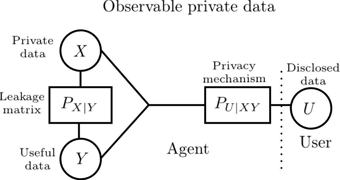
Figure 1: Considered scenario where the agent has access to both $X$ and $Y$.

II system model and Problem Formulation

Let $P_{XY}$ denote the joint distribution of discrete random variables $X$ and $Y$ defined on alphabets $\cal{X}$ and $\cal{Y}$. We assume that cardinality $|\mathcal{X}|$ is finite and $|\mathcal{Y}|$ is finite or countably infinite. We represent $P_{XY}$ by a matrix defined on $\mathbb{R}^{|\mathcal{X}|\times|\mathcal{Y}|}$ and marginal distributions of $X$ and $Y$ by vectors $P_{X}$ and $P_{Y}$ defined on $\mathbb{R}^{|\mathcal{X}|}$ and $\mathbb{R}^{|\mathcal{Y}|}$ given by the row and column sums of $P_{XY}$. We represent the leakage matrix $P_{X|Y}$ by a matrix defined on $\mathbb{R}^{|\mathcal{X}|\times|\cal{Y}|}$.

Here, we use mutual information as utility and leakage measures. The privacy mechanism design problem can be stated as follows

$$h_{\epsilon}(P_{XY}) =\sup_{\begin{array}[]{c}\begin{subarray}{c}P_{U|Y,X}:I(U;X)\leq\epsilon,\end{subarray}\end{array}}I(Y;U).$$ (2)

The relation between $U$ and the pair $(Y,X)$ is described by the kernel $P_{U|Y,X}$ defined on $\mathbb{R}^{|\mathcal{U}|\times|\mathcal{Y}|\times|\mathcal{X}|}$. In the following we study the case where $0\leq\epsilon<I(X;Y)$, otherwise the optimal solution of $h_{\epsilon}(P_{XY})$ is $H(Y)$ achieved by $U=Y$.

Remark 1.

For $\epsilon=0$, (2) leads to the secret-dependent perfect privacy function $h_{0}(P_{XY})$, studied in [8], where upper and lower bounds on $h_{0}(P_{XY})$ have been derived. The bounds are generalized in [9].

III Main Results

In this section, we first recall the Functional Representation Lemma (FRL) [8, Lemma 1], Strong Functional Representation Lemma (SFRL) [20, Theorem 1], Extended Functional Representation Lemma (EFRL) [9, Lemma 3], and Extended Strong Functional Representation Lemma (ESFRL) [9, Lemma 4], for discrete $X$ and $Y$. We then present a simple but important result regarding representing a RV by two correlated RVs.

Lemma 1.

(Functional Representation Lemma [8, Lemma 1]): For any pair of RVs $(X,Y)$ distributed according to $P_{XY}$ supported on alphabets $\mathcal{X}$ and $\mathcal{Y}$ where $|\mathcal{X}|$ is finite and $|\mathcal{Y}|$ is finite or countably infinite, there exists a RV $U$ supported on $\mathcal{U}$ such that $X$ and $U$ are independent, i.e., we have

$$I(U;X)=0,$$ (3)

$Y$ is a deterministic function of $(U,X)$, i.e., we have

$$H(Y|U,X)=0,$$ (4)

and

$$|\mathcal{U}|\leq|\mathcal{X}|(|\mathcal{Y}|-1)+1.$$ (5)

Lemma 2.

(Strong Functional Representation Lemma [20, Theorem 1]): For any pair of RVs $(X,Y)$ distributed according to $P_{XY}$ supported on alphabets $\mathcal{X}$ and $\mathcal{Y}$ where $|\mathcal{X}|$ is finite and $|\mathcal{Y}|$ is finite or countably infinite with $I(X,Y)<\infty$, there exists a RV $U$ supported on $\mathcal{U}$ such that $X$ and $U$ are independent, i.e., we have

$$I(U;X)=0,$$

$Y$ is a deterministic function of $(U,X)$, i.e., we have

$$H(Y|U,X)=0,$$

$I(X;U|Y)$ can be upper bounded as follows

$$I(X;U|Y)\leq\log(I(X;Y)+1)+4,$$

and $|\mathcal{U}|\leq|\mathcal{X}|(|\mathcal{Y}|-1)+2.$

Lemma 3.

(Extended Functional Representation Lemma [9, Lemma 3]): For any $0\leq\epsilon<I(X;Y)$ and pair of RVs $(X,Y)$ distributed according to $P_{XY}$ supported on alphabets $\mathcal{X}$ and $\mathcal{Y}$ where $|\mathcal{X}|$ is finite and $|\mathcal{Y}|$ is finite or countably infinite, there exists a RV $U$ supported on $\mathcal{U}$ such that the leakage between $X$ and $U$ is equal to $\epsilon$, i.e., we have

$$I(U;X)=\epsilon,$$

$Y$ is a deterministic function of $(U,X)$, i.e., we have

$$H(Y|U,X)=0,$$

and $|\mathcal{U}|\leq\left[|\mathcal{X}|(|\mathcal{Y}|-1)+1\right]\left[|\mathcal{X}|+1\right].$

Proof.

The proof is based on adding a randomized response to the output of the FRL. The randomized response has been introduced in [21]. ∎

Lemma 4.

(Extended Strong Functional Representation Lemma [9, Lemma 4]): For any $0\leq\epsilon<I(X;Y)$ and pair of RVs $(X,Y)$ distributed according to $P_{XY}$ supported on alphabets $\mathcal{X}$ and $\mathcal{Y}$ where $|\mathcal{X}|$ is finite and $|\mathcal{Y}|$ is finite or countably infinite with $I(X,Y)<\infty$, there exists a RV $U$ supported on $\mathcal{U}$ such that the leakage between $X$ and $U$ is equal to $\epsilon$, i.e., we have

$$I(U;X)=\epsilon,$$

$Y$ is a deterministic function of $(U,X)$, i.e., we have

$$H(Y|U,X)=0,$$

$I(X;U|Y)$ can be upper bounded as follows

$$I(X;U|Y)\leq\alpha H(X|Y)+(1-\alpha)\left[\log(I(X;Y)+1)+4\right],$$

and $|\mathcal{U}|\leq\left[|\mathcal{X}|(|\mathcal{Y}|-1)+2\right]\left[|\mathcal{X}|+1\right],$ where $\alpha=\frac{\epsilon}{H(X)}$.

Proof.

Similar to EFRL, the proof is based on adding a randomized response to the output of the SFRL. ∎

Next, we present a simple observation which we call “separation technique”.

Observation.

(Separation technique) Any discrete RV $X$ supported on $\mathcal{X}=\{1,\ldots,|\mathcal{X}|\}$ can be represented by two RVs $(X_{1},X_{2})$.

Proof.

First, let $|\mathcal{X}|$ be not a prime number. Thus, there exist $|\mathcal{X}_{1}|$ and $|\mathcal{X}_{2}|$ such that $|\mathcal{X}|=|\mathcal{X}_{1}|\times|\mathcal{X}_{2}|$ where $|\mathcal{X}_{1}|\geq|\mathcal{X}_{2}|\geq 2$. We can uniquely map each $x\in\mathcal{X}$ into a pair $(x_{1},x_{2})$ where $x_{1}\in\mathcal{X}_{1}$ and $x_{2}\in\mathcal{X}_{2}$. As a result, we can represent $X$ by the pair $(X_{1},X_{2})$ where $\mathcal{X}_{1}=\{1,\ldots,|\mathcal{X}_{1}|\}$, $\mathcal{X}_{2}=\{1,\ldots,|\mathcal{X}_{2}|\}$, and $P_{X}(x)=P_{X_{1}X_{2}}(x_{1},x_{2})$. Next, let $|\mathcal{X}|$ be a prime number. Hence, there exist $|\mathcal{X}_{1}|$ and $|\mathcal{X}_{2}|$ such that $|\mathcal{X}|+1=|\mathcal{X}_{1}|\times|\mathcal{X}_{2}|$ and we can represent $X$ by the pair $(X_{1},X_{2})$ where $P_{X_{1}X_{2}}(x_{1}=|\mathcal{X}_{1}|,x_{2}=|\mathcal{X}_{2}|)=0$. In other words, the last pair $(|\mathcal{X}_{1}|,|\mathcal{X}_{2}|)$ is not mapped to any $x\in\mathcal{X}$. ∎

Remark 2.

The representation obtained by the separation technique is not unique. For instance, let $|\mathcal{X}|=16$. In this case, $|\mathcal{X}_{1}|=4$, $|\mathcal{X}_{2}|=4$ or $|\mathcal{X}_{1}|=8$, $|\mathcal{X}_{2}|=2$.

We define $\mathcal{S}_{X}$ as all possible representations of $X$ where $X=(X_{1},X_{2})$. In other words we have $\mathcal{S}_{X}=\{(X_{1},X_{2}):X=(X_{1},X_{2}),\ |\mathcal{X}_{1}|\geq 2,\ |\mathcal{X}_{2}|\geq 2\}$.

Before stating the next theorem we derive an expression for $I(Y;U)$. We have

$$I(Y;U) =I(X,Y;U)-I(X;U|Y),$$

$$=I(X;U)+I(Y;U|X)-I(X;U|Y),$$

$$=I(X;U)\!+\!H(Y|X)\!-\!H(Y|U,X)\!-\!I(X;U|Y).$$ (6)

As argued in [8], (6) is an important observation to find lower and upper bounds for $h_{\epsilon}(P_{XY})$. Next, we derive lower and upper bounds on $h_{\epsilon}(P_{XY})$. For deriving new lower bounds we use EFRL, ESFRL combining with separation technique.

Theorem 1.

For any $0\leq\epsilon<I(X;Y)$ and pair of RVs $(X,Y)$ distributed according to $P_{XY}$ supported on alphabets $\mathcal{X}$ and $\mathcal{Y}$ we have

$$\max\{L_{1}^{\epsilon},L_{2}^{\epsilon},L_{3}^{\epsilon},L_{4}^{\epsilon},L_{5}^{\epsilon}\}\leq h_{\epsilon}(P_{XY})\leq U_{1}^{\epsilon},$$ (7)

where

$$U_{1}^{\epsilon} =H(Y|X)-\epsilon,$$

$$L_{1}^{\epsilon} =H(Y|X)-H(X|Y)+\epsilon=H(Y)-H(X)+\epsilon,$$

$$L_{2}^{\epsilon} =H(Y|X)-\alpha H(X|Y)+\epsilon$$

$$\ -(1-\alpha)\left(\log(I(X;Y)+1)+4\right),$$

$$L_{3}^{\epsilon} =\epsilon\frac{H(Y)}{I(X;Y)}+g_{0}(P_{XY})\left(1-\frac{\epsilon}{I(X;Y)}\right),$$

$$L_{4}^{\epsilon} =H(Y|X)+\epsilon-\left(\log(I(X;Y)+1)+4\right)$$

$$-\min_{(X_{1},X_{2})\in\mathcal{S}_{X}}\{\alpha_{2}H(X_{2}|Y)\},$$

$$L_{5}^{\epsilon} =H(Y|X)+\epsilon$$

$$-\!\!\!\!\!\!\!\!\min_{(X_{1},X_{2})\in\mathcal{S}_{X}}\!\!\!\{(1\!-\!\alpha_{2})\!\left(\log(I(X;Y)\!+\!1)\!+\!4\right)\!+\!\alpha_{2}H(X|Y)\},$$

and $\alpha=\frac{\epsilon}{H(X)}$, $\alpha_{2}=\frac{\epsilon}{H(X_{2})}$ for any representation $X=(X_{1},X_{2})$. Furthermore, $g_{0}(P_{XY})=\max_{\begin{array}[]{c}\begin{subarray}{c}P_{U|Y,X}:I(U;X)=0,\\ X-Y-U\end{subarray}\end{array}}I(Y;U).$ The lower bound in (7) is tight if $H(X|Y)=0$, i.e., $X$ is a deterministic function of $Y$. Furthermore, if the lower bound $L_{1}$ is tight then we have $H(X|Y)=0$.

Proof.

The lower bound $L_{3}^{\epsilon}$ can be derived by using [19, Remark 2], since we have $h_{\epsilon}(P_{XY})\geq g_{\epsilon}(P_{XY})\geq L_{3}^{\epsilon}$, where $g_{\epsilon}(P_{XY})=\sup_{\begin{array}[]{c}\begin{subarray}{c}P_{U|Y,X}:I(U;X)\leq\epsilon,\\ X-Y-U\end{subarray}\end{array}}I(Y;U)$. The upper bound $U_{1}^{\epsilon}$ and lower bounds $L_{1}^{\epsilon}$ and $L_{2}^{\epsilon}$ have been derived in [9, Theorem 2]. The lower bound $L_{1}^{\epsilon}$ is attained by using (6) and EFRL. Similarly, the lower bound $L_{2}^{\epsilon}$ is attained by (6) and ESFRL, for more detail see [9, Theorem 2]. Moreover, the results about tightness have been proved in [9, Theorem 2]. It is sufficient to obtain $L_{4}^{\epsilon}$ and $L_{5}^{\epsilon}$. The complete proof for obtaining $L_{4}^{\epsilon}$ and $L_{5}^{\epsilon}$ is provided in Appendix A. As we mentioned earlier to achieve $L_{1}^{\epsilon}$ or $L_{2}^{\epsilon}$ we use EFRL or ESFRL. The main idea for constructing a RV $U$ that satisfies EFRL or ESFRL constraints is to add a randomized response to the output of FRL or SFRL. The randomization is taken over $X$. Now, let $(X_{1},X_{2})$ be a possible representation of $X$, i.e., $X=(X_{1},X_{2})$. The main idea to achieve $L_{4}^{\epsilon}$ and $L_{5}^{\epsilon}$ is to take randomization over $X_{2}$ instead of $X$. In other words we add a randomized response which is based on $X_{2}$ instead of $X$. Considering $L_{2}^{\epsilon}$ and $L_{4}^{\epsilon}$, $\alpha$ corresponds to the probability of randomizing over $X$, however, $\alpha_{2}$ corresponds to the probability of randomizing over $X_{2}$ for any representation $X=(X_{1},X_{2})$. ∎

In next corollary we let $\epsilon=0$ and derive lower bound on $h_{0}(P_{XY})$.

Remark 3.

We emphasize that the lower bounds $L_{1}^{\epsilon}$, $L_{2}^{\epsilon}$, and $L_{3}^{\epsilon}$ have been derived in [8], [9], and [19], respectively, however, the lower bounds $L_{4}^{\epsilon}$ and $L_{5}^{\epsilon}$ are obtained in this work.

Remark 4.

The lower bounds $L_{1}^{\epsilon}$, $L_{2}^{\epsilon}$, $L_{4}^{\epsilon}$, and $L_{5}^{\epsilon}$ have constructive proofs. Hence, statistical privacy mechanisms can be obtained using the lower bounds. For instance, RV $U$ that attains $L_{4}^{\epsilon}$ is built based on separation technique and extended version of SFRL. Noting that EFRL and ESFRL have also constructive proofs.

Corollary 1.

([9, Corollary 2]) If $X$ is a deterministic function of $Y$, the upper bound $U_{1}^{\epsilon}$ is attained.

Corollary 2.

Let $\epsilon=0$. In this case we obtain the same results as [9, Corllary 1], since $L_{4}^{0}=L_{5}^{0}=L_{2}^{0}$. For any pair of RVs $(X,Y)$ distributed according to $P_{XY}$ supported on alphabets $\mathcal{X}$ and $\mathcal{Y}$ we have

$$h_{0}(P_{XY})\geq\max\{L^{0}_{1},L^{0}_{2},g_{0}(P_{XY})\},$$

where

$$L^{0}_{1} =H(Y|X)-H(X|Y)=H(Y)-H(X),$$

$$L^{0}_{2} =H(Y|X)-\left(\log(I(X;Y)+1)+4\right).$$

Note that the lower bounds $L_{4}^{\epsilon}$ and $L_{5}^{\epsilon}$ do not lead to new bounds for $\epsilon=0$, however, for non-zero leakage they can improve the previous bounds.

IV comparison

In this part we study the bounds considering different cases. For simplicity let $X=(X_{1},X_{2})$ where $X_{1}$ and $X_{2}$ are arbitrary correlated. In this case we have

$$U_{1}^{\epsilon} =H(Y|X_{1},X_{2})-\epsilon,$$

$$L_{1}^{\epsilon} =H(Y|X_{1},X_{2})-H(X_{1},X_{2}|Y)+\epsilon,$$

$$L_{2}^{\epsilon} =H(Y|X_{1},X_{2})-\alpha H(X_{1},X_{2}|Y)+\epsilon$$

$$\ -(1-\alpha)\left(\log(I(X_{1},X_{2};Y)+1)+4\right),$$

$$L_{3}^{\epsilon} =\epsilon\frac{H(Y)}{I(X_{1},X_{2};Y)}+g_{0}(P_{XY})\left(1-\frac{\epsilon}{I(X_{1},X_{2};Y)}\right),$$

$$L_{4}^{\epsilon} =H(Y|X_{1},X_{2})+\epsilon-\left(\log(I(X_{1},X_{2};Y)+1)+4\right)$$

$$-\alpha_{2}H(X_{2}|Y),$$

$$L_{5}^{\epsilon} =H(Y|X_{1},X_{2})+\epsilon$$

$$\!\!\!\!\!\!\!\!-(1\!-\!\alpha_{2})\!\left(\log(I(X_{1},X_{2};\!Y)\!+\!1)\!+\!4\right)\!+\!\alpha_{2}H(X_{1},X_{2}|Y),$$

where $\alpha=\frac{\epsilon}{H(X)}$ and $\alpha_{2}=\frac{\epsilon}{H(X_{2})}$. We first compare the lower bounds $L_{1}^{\epsilon}$, $L_{4}^{\epsilon}$, and $L_{5}^{\epsilon}$. To do so, we consider four scenarios as follows.
Scenario 1: Let $X_{1}$ be a deterministic function of $Y$, i.e., $H(X_{1}|Y)=0$. Consequently, $L_{1}^{\epsilon}$ is dominant and we have $L_{1}^{\epsilon}\geq L_{5}^{\epsilon}\geq L_{4}^{\epsilon}$, since in this case $H(X_{1},X_{2}|Y)=H(X_{2}|Y)$.
Scenario 2: Let $4+H(Y)\leq H(X_{1}|Y)$ and assume that $X_{2}$ is a deterministic function of $Y$, i.e., $H(X_{2}|Y)=0$. In this case, we have

$$L_{4}^{\epsilon}\!-\!L_{5}^{\epsilon}\! =\!\alpha_{2}\!\left(H(X_{1}|Y\!)\!-\!\log(I(X_{1};Y\!)\!+\!H(X_{2}|X_{1}\!)\!+\!1)\!-\!4\right)$$

$$\stackrel{{\scriptstyle(a)}}{{\geq}}\alpha_{2}\left(H(X_{1}|Y)-I(X_{1};Y)-H(X_{2}|X_{1})-4\right)$$

$$\stackrel{{\scriptstyle(b)}}{{\geq}}\alpha_{2}\left(H(X_{1}|Y)-I(X_{1};Y)-H(Y|X_{1})-4\right)$$

$$=\alpha_{2}\left(H(X_{1}|Y)-H(Y)-4\right)$$

$$\geq 0,$$ (8)

where (a) follows since $\log(1+x)\leq x$ and (b) holds since we have $H(X_{2}|X_{1})\leq H(Y|X_{1})$ and $H(X_{2}|Y)=0$. Furthermore,

$$L_{4}^{\epsilon}\!-\!L_{1}^{\epsilon} \!=\!H(X_{1}|Y)\!-\!\log(I(X_{1};Y)\!+\!H(X_{2}|X_{1})\!+\!1)\!-\!4$$

$$\geq H(X_{1}|Y)-I(X_{1};Y)-H(X_{2}|X_{1})-4$$

$$\geq H(X_{1}|Y)-I(X_{1};Y)-H(Y|X_{1})-4$$

$$=H(X_{1}|Y)-H(Y)-4$$

$$\geq 0.$$ (9)

So, in this scenario $L_{4}^{\epsilon}$ is dominant and we have $L_{4}^{\epsilon}\geq\max(L_{1}^{\epsilon},L_{5}^{\epsilon})$.
Scenario 3: Let $H(X_{1},X_{2})\geq 4$ and $Y$ be independent of $(X_{1},X_{2})$. In this case we have $L_{4}^{\epsilon}\geq L_{1}^{\epsilon}$ and $L_{5}^{\epsilon}\geq L_{1}^{\epsilon}$.
Scenario 4: Let $H(X_{2}|Y)\geq\log(I(X_{2};Y)+1)+4$ and $X_{1}$ be a deterministic function of $X_{2}$. A simple example can be letting $X_{1}=f(X_{2})$ and $H(X_{2}|Y)\geq\frac{H(X_{2})}{2}+2$ which results in $H(X_{2}|Y)\geq\log(I(X_{2};Y)+1)+4$ using $\log(x+1)\leq x$. We have

$$L_{5}^{\epsilon}-L_{4}^{\epsilon} =\epsilon\frac{H(X_{2}|Y)}{H(X_{2})}$$

$$+\epsilon\frac{\log(I(X_{2};Y)+1)+4}{H(X_{2})}-\epsilon\frac{H(X_{2}|Y)}{H(X_{2})}$$

$$=\epsilon\frac{\log(I(X_{2};Y)+1)+4}{H(X_{2})}\geq 0.$$

Furthermore,

$$L_{5}^{\epsilon}-L_{1}^{\epsilon}=$$

$$(1-\alpha)\left[H(X_{2}|Y)-\log(I(X_{2};Y)+1)-4\right]\geq 0.$$

Hence, in this case $L_{5}^{\epsilon}$ is dominant and we have $L_{5}^{\epsilon}\geq\max\{L_{4}^{\epsilon},L_{1}^{\epsilon}\}$.
We next compare the lower bounds $L_{2}^{\epsilon}$, $L_{4}^{\epsilon}$, and $L_{5}^{\epsilon}$. To do so we consider the following scenarios.
Scenario 1: To compare $L_{5}^{\epsilon}$ with $L_{2}^{\epsilon}$, let us assume that $H(X_{1},X_{2}|Y)\leq\log(I(X_{1},X_{2};Y)+1)+4$. A simple example can be considering $X_{1}$ and $X_{2}$ as binary RVs. In this case we have

$$L_{5}^{\epsilon}-L_{2}^{\epsilon}=\epsilon(\frac{1}{H(X_{2})}-\frac{1}{H(X_{1},X_{2})})\times$$

$$\left(\log(I(X_{1},X_{2};Y)+1)+4-H(X_{1},X_{2}|Y)\right)\geq 0.$$

Scenario 2: To compare $L_{4}^{\epsilon}$ with $L_{2}^{\epsilon}$, let us assume that $X_{2}$ is a deterministic function of $Y$ and $H(X_{1}|Y)\geq\log(I(X_{1},X_{2};Y)+1)+4$. As we pointed out earlier a simple example is to let $4+H(Y)\leq H(X_{1}|Y)$ which leads to $H(X_{1}|Y)\geq\log(I(X_{1},X_{2};Y)+1)+4$. In this case we have

$$L_{4}^{\epsilon}-L_{2}^{\epsilon}=$$

$$\frac{\epsilon}{H(X_{1},X_{2})}\left(H(X_{1}|Y)\!-\!\log(I(X_{1},X_{2};Y)+1)-4\right)\geq 0.$$

Moreover, by using (8) and (9) we conclude that $L_{4}^{\epsilon}$ is dominant and we have

$$L_{4}^{\epsilon}\geq\max\{L_{2}^{\epsilon},L_{5}^{\epsilon},L_{1}^{\epsilon}\}.$$

V conclusion

We have introduced separation technique and it has been shown that combining it with extended versions of the FRL and SFRL, lead to new lower bounds on $h_{\epsilon}(P_{XY})$. If $X$ is a deterministic function of $Y$, then the bounds are tight. In different scenarios it has been shown that new bounds are dominant compared to the previous bounds.

Appendix A

Deriving lower bounds $L_{4}^{\epsilon}$ and $L_{5}^{\epsilon}$:

Let $(X_{1},X_{2})\in\mathcal{S}_{X}$, i.e., $(X_{1},X_{2})$ be a possible representation of $X$. The bounds $L_{4}^{\epsilon}$ and $L_{5}^{\epsilon}$ can be obtained as follows. Let $\bar{U}$ be found by SFRL with $X=(X_{1},X_{2})$. We have

$$I(\bar{U};X_{1},X_{2}) =0,$$

$$H(Y|\bar{U},X_{1},X_{2}) =0,$$

$$I(X_{1},X_{2};\bar{U}|Y) \leq\log(I(X_{1},X_{2};Y)+1)+4.$$

Moreover, let $U=(\bar{U},W)$ with $W=\begin{cases}X_{2},\ \text{w.p}.\ \alpha_{2}\\ c,\ \ \text{w.p.}\ 1-\alpha_{2}\end{cases}$, where $c$ is a constant which does not belong to $\mathcal{X}_{1}\cup\mathcal{X}_{2}\cup\mathcal{Y}$ and $\alpha_{2}=\frac{\epsilon}{H(X_{2})}$. First we show that $I(U;X_{1},X_{2})=\epsilon$. We have

$$I(U;X_{1},X_{2}) =I(\bar{U},W;X_{1},X_{2})\stackrel{{\scriptstyle(a)}}{{=}}I(W;X_{1},X_{2})$$

$$=\!H\!(X_{1},\!X_{2})\!-\!\alpha_{2}H(X_{1}|X_{2})\!$$

$$-\!(1\!-\!\alpha_{2})H\!(X_{1},\!X_{2})$$

$$=\alpha H(X_{2})$$

$$=\epsilon,$$

where (a) follows since $\bar{U}$ is independent of $(X_{1},X_{2},W)$. Next, we expand $I(U;X_{1},X_{2}|Y)$.

$$I(U;X_{1},X_{2}|Y)$$ (10)

$$=I(\bar{U};X_{1},X_{2}|Y)+I(W;X_{1},X_{2}|Y,\bar{U})$$

$$=I(\bar{U};X_{1},X_{2}|Y)+H(X_{1},X_{2}|Y,\bar{U})\!$$ (11)

$$-\!H(X_{1},X_{2}|Y,\bar{U},W)$$

$$=I(\bar{U};X_{1},X_{2}|Y)+\alpha_{2}H(X_{1},X_{2}|Y,\bar{U})$$ (12)

$$-\alpha_{2}H(X_{1}|Y,\bar{U},X_{2})$$

$$=I(\bar{U};X_{1},X_{2}|Y)-\alpha_{2}H(X_{1}|Y,\bar{U},X_{2})$$ (13)

$$+\alpha_{2}\left(H(X_{1},X_{2}|Y)-I(\bar{U};X_{1},X_{2}|Y)\right)$$

$$=\!(1\!-\!\alpha)I(\bar{U};X_{1},\!X_{2}|Y)\!+\!\alpha_{2}H(X_{1},X_{2}|Y)$$

$$-\!\alpha_{2}H(X_{1}|Y\!,\!\bar{U}\!,\!X_{2}).$$ (14)

In the following we bound (14) in two ways. We have

$$\eqref{jakesh} =\!(1\!-\!\alpha_{2})I(\bar{U};X_{1},\!X_{2}|Y)\!+\!\alpha_{2}H(X_{2}|Y)$$ (15)

$$+\alpha I(X_{1};\bar{U}|Y,X_{2})$$

$$=I(\bar{U};X_{1},\!X_{2}|Y)\!+\!\alpha_{2}H(X_{2}|Y)\!-\!\alpha_{2}I(\bar{U};X_{2}|Y)$$

$$\stackrel{{\scriptstyle(a)}}{{\leq}}\log(I(X_{1},X_{2};Y)+1)+4+\alpha_{2}H(X_{2}|Y).$$ (16)

Furthermore,

$$\eqref{jakesh} \leq\!(1\!-\!\alpha_{2})I(\bar{U};X_{1},\!X_{2}|Y)+\alpha_{2}H(X_{1},\!X_{2}|Y\!)$$

$$\stackrel{{\scriptstyle(b)}}{{\leqq}}\!(1\!-\!\alpha_{2})\left(\log(I(X_{1},X_{2};Y)+1)+4\right)$$

$$+\alpha_{2}H(X_{1},\!X_{2}|Y\!).$$ (17)

Inequalities (a) and (b) follow since $\bar{U}$ is produced by SFRL, so that $I(\bar{U};X_{1},X_{2}|Y)\leq\log(I(X_{1},X_{2};Y)+1)+4$. Using (16), (17) and key equation in (6) we have

$$h_{\epsilon}(P_{XY}) \geq I(U;Y)$$

$$\stackrel{{\scriptstyle(c)}}{{\geq}}\epsilon+H(Y|X_{1},X_{2})-\alpha_{2}H(X_{2}|Y)$$

$$-\left(\log(I(X_{1},X_{2};Y)+1)+4\right)$$

$$=\epsilon+H(Y|X)-\alpha_{2}H(X_{2}|Y)$$

$$-\left(\log(I(X_{1},X_{2};Y)+1)+4\right),$$ (18)

and

$$h_{\epsilon}(P_{XY}) \geq I(U;Y)$$

$$\stackrel{{\scriptstyle(d)}}{{\geq}}\epsilon+H(Y|X_{1},X_{2})-\alpha_{2}H(X_{1},X_{2}|Y)$$

$$-(1-\alpha_{2})(\log(I(X_{1},X_{2};Y)+1)+4)$$

$$=\epsilon+H(Y|X)-\alpha_{2}H(X|Y)$$

$$-(1-\alpha_{2})(\log(I(X;Y)+1)+4).$$ (19)

In steps (c) and (d) we used $H(Y|X_{1},X_{2},U)=0$. The latter follows by definition of $W$ and the fact that $\bar{U}$ is produced by SFRL. Noting that since both (18) and (19) hold for any representation of $X$ we can take maximum over all possible representations and we obtain

$$h_{\epsilon}(P_{XY})\geq H(Y|X)+\epsilon-\left(\log(I(X;Y)+1)+4\right)$$

$$-\min_{(X_{1},X_{2})\in\mathcal{S}_{X}}\{\alpha_{2}H(X_{2}|Y)\}=L_{4}^{\epsilon},$$

$$h_{\epsilon}(P_{XY})\geq H(Y|X)+\epsilon$$

$$-\!\!\!\!\!\!\!\!\min_{(X_{1},X_{2})\in\mathcal{S}_{X}}\!\!\!\{(1\!-\!\alpha_{2})\!\left(\log(I(X;Y)\!+\!1)\!+\!4\right)\!+\!\alpha_{2}H(X|Y)\}$$

$$=L_{5}^{\epsilon}.$$

References

- [1] H. Wang, L. Vo, F. P. Calmon, M. Médard, K. R. Duffy, and M. Varia, “Privacy with estimation guarantees,” IEEE Transactions on Information Theory, vol. 65, no. 12, pp. 8025–8042, Dec 2019.
- [2] H. Yamamoto, “A source coding problem for sources with additional outputs to keep secret from the receiver or wiretappers (corresp.),” IEEE Transactions on Information Theory, vol. 29, no. 6, pp. 918–923, 1983.
- [3] L. Sankar, S. R. Rajagopalan, and H. V. Poor, “Utility-privacy tradeoffs in databases: An information-theoretic approach,” IEEE Transactions on Information Forensics and Security, vol. 8, no. 6, pp. 838–852, 2013.
- [4] B. Rassouli and D. Gündüz, “On perfect privacy,” IEEE Journal on Selected Areas in Information Theory, vol. 2, no. 1, pp. 177–191, 2021.
- [5] S. Sreekumar and D. Gündüz, “Optimal privacy-utility trade-off under a rate constraint,” in 2019 IEEE International Symposium on Information Theory, July 2019, pp. 2159–2163.
- [6] A. Zamani, T. J. Oechtering, and M. Skoglund, “A design framework for strongly -private data disclosure,” IEEE Transactions on Information Forensics and Security, vol. 16, pp. 2312–2325, 2021.
- [7] A. Zamani, T. J. Oechtering, and M. Skoglund, “Data disclosure with non-zero leakage and non-invertible leakage matrix,” IEEE Transactions on Information Forensics and Security, vol. 17, pp. 165–179, 2022.
- [8] Y. Y. Shkel, R. S. Blum, and H. V. Poor, “Secrecy by design with applications to privacy and compression,” IEEE Transactions on Information Theory, vol. 67, no. 2, pp. 824–843, 2021.
- [9] A. Zamani, T. J. Oechtering, and M. Skoglund, “Bounds for privacy-utility trade-off with non-zero leakage,” in 2022 IEEE International Symposium on Information Theory (ISIT), 2022, pp. 620–625.
- [10] I. Issa, S. Kamath, and A. B. Wagner, “An operational measure of information leakage,” in 2016 Annual Conference on Information Science and Systems, March 2016, pp. 234–239.
- [11] A. Makhdoumi, S. Salamatian, N. Fawaz, and M. Médard, “From the information bottleneck to the privacy funnel,” in 2014 IEEE Information Theory Workshop, 2014, pp. 501–505.
- [12] C. Dwork, F. McSherry, K. Nissim, and A. Smith, “Calibrating noise to sensitivity in private data analysis,” in Theory of cryptography conference. Springer, 2006, pp. 265–284.
- [13] F. P. Calmon, A. Makhdoumi, M. Medard, M. Varia, M. Christiansen, and K. R. Duffy, “Principal inertia components and applications,” IEEE Transactions on Information Theory, vol. 63, no. 8, pp. 5011–5038, Aug 2017.
- [14] I. Issa, A. B. Wagner, and S. Kamath, “An operational approach to information leakage,” IEEE Transactions on Information Theory, vol. 66, no. 3, pp. 1625–1657, 2020.
- [15] S. Asoodeh, M. Diaz, F. Alajaji, and T. Linder, “Estimation efficiency under privacy constraints,” IEEE Transactions on Information Theory, vol. 65, no. 3, pp. 1512–1534, 2019.
- [16] B. Rassouli and D. Gündüz, “Optimal utility-privacy trade-off with total variation distance as a privacy measure,” IEEE Transactions on Information Forensics and Security, vol. 15, pp. 594–603, 2020.
- [17] B. Rassouli, F. E. Rosas, and D. Gündüz, “Data disclosure under perfect sample privacy,” IEEE Transactions on Information Forensics and Security, pp. 1–1, 2019.
- [18] I. Issa, S. Kamath, and A. B. Wagner, “Maximal leakage minimization for the shannon cipher system,” in 2016 IEEE International Symposium on Information Theory, 2016, pp. 520–524.
- [19] S. Asoodeh, M. Diaz, F. Alajaji, and T. Linder, “Information extraction under privacy constraints,” Information, vol. 7, no. 1, 2016. [Online]. Available: https://www.mdpi.com/2078-2489/7/1/15
- [20] C. T. Li and A. El Gamal, “Strong functional representation lemma and applications to coding theorems,” IEEE Transactions on Information Theory, vol. 64, no. 11, pp. 6967–6978, 2018.
- [21] S. L. Warner, “Randomized response: A survey technique for eliminating evasive answer bias,” Journal of the American Statistical Association, vol. 60, no. 309, pp. 63–69, 1965.