Active shape control by plants in dynamic environments

Abstract

Plants are a paradigm for active shape control in response to stimuli. For instance, it is well-known that a tilted plant will eventually straighten vertically, demonstrating the influence of both an external stimulus, gravity, and an internal stimulus, proprioception. These effects can be modulated when a potted plant is additionally rotated along the plant’s axis, as in a rotating clinostat, leading to intricate shapes. We use a morphoelastic model for the response of growing plants to study the joint effect of both stimuli at all rotation speeds. In the absence of rotation, we identify a universal planar shape towards which all shoots eventually converge. With rotation, we demonstrate the existence of a stable family of three-dimensional dynamic equilibria where the plant axis is fixed in space. Further, the effect of axial growth is to induce steady behaviors, such as solitary waves. Overall, this study offers new insight into the complex out-of-equilibrium dynamics of a plant in three dimensions and further establishes that internal stimuli in active materials are key for robust shape control.

Active materials are characterized by their ability to adapt to external stimuli, often manifested by changes in shape. A paradigm of this adaptability is observed in the growth patterns of plant shoots, which exhibit remarkable sensitivity not only to their environment (e.g. light, gravity, wind) [1] but also, intriguingly, to their own evolving shapes, a phenomenon called proprioception [2, 3]. We show that this synergistic response to multiple stimuli serves as a robust mechanism for plants to maintain structural integrity in highly dynamic environments. An important type of response in plant shoots is gravitropism [Fig. 1(a)], the tendency to react and orient their growth against the direction of gravity [4]. While modifying gravity experimentally is challenging, it is possible to nullify its influence by rotating the plant sufficiently fast in a clinostat [5], shown in Fig. 1(b). This device, patented by Julius von Sachs circa 1880 [6, 7], imparts a constant rotational motion to the plant, thereby cyclically altering the relative direction of gravity. To simulate weightlessness, the clinostat must rotate at a relatively high angular speed $\omega$, compared to the response of the plant, allowing for the averaging out of gravity’s influence over multiple rotations [8]. In such a case, the plant grows straight. Further, the general observation that growing shoots tend to straighten in the absence of other influences, indicates another well-established necessary response, called autotropism, the tendency to minimize curvature during growth [9]. Under slower rotations, the relative influence of autotropism and gravitropism can be gauged by varying the angular speed, leading to the possibility of complex three-dimensional shapes that we study here.

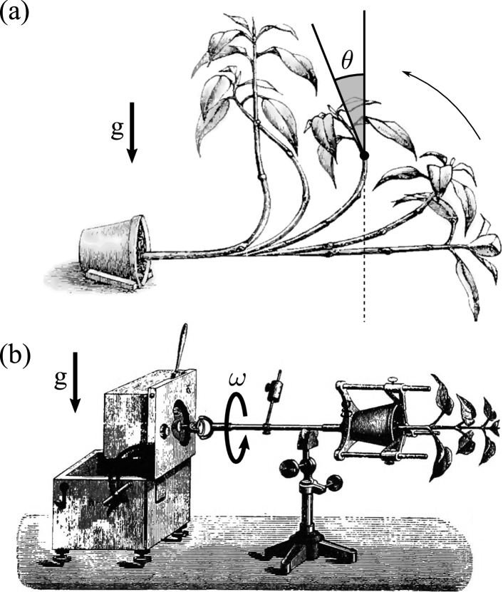
Figure 1: (a) A potted plant realigns itself with gravity when tilted horizontally. (b) In a clinostat, the effect of gravity is nullified at sufficient angular speed. In both cases, the plant’s axis lies in a plane. (Adapted from [10])

The first model for the gravitropic response of slender shoots was formulated by Sachs in 1879 [7]. The sine law states that the rate of change of curvature at a point is given by the sine of the inclination angle $\theta({s,t})$ between the tangent to the shoot centerline and the vertical direction, where $s$ is the arclength from the base and $t$ is the time [Fig. 1(a)]. Recalling that the curvature is the arclength derivative of this angle, the sine law can be expressed as

$$\dot{\theta}^{\prime}+\alpha\sin\theta=0,$$ (1)

with $\alpha$ a rate constant; and where $(\ )^{\prime}$ and $\dot{(\ )}$ denote differentiation w.r.t. $s$ and $t$, respectively. Notably, unbeknownst to Sachs and his successors, the sine law is an instance of the celebrated sine-Gordon equation, a fully integrable system with a conservative structure [11]; in fact, the sine law is the earliest appearance of this equation as a physical model. While the sine law is the starting point of many augmented models [9, 12, 13, 14, 15, 16], it is restricted to planar motion and does not include autotropism, which is necessary for shoots to eventually straighten [9, 17].

Here, we follow the plant tropism framework developed in [1] to model the clinostatting plant in three dimensions as an unshearable and inextensible morphoelastic rod [18, 19] of length $\ell$. We neglect self-weight and centrifugal effects, which is valid for small shoots and slow rotation (i.e. $\rho g\ell^{3}\ll B$ and $\rho\omega^{2}\ell^{4}\ll B$, with $B$ and $\rho$ denoting the bending stiffness and the linear density, respectively). In this case, the shoot assumes its stress-free shape. In the first scenario studied here, we also neglect the axial growth of the shoot and focus on curvature generation through tissue growth and remodeling. Thus, the shoot has a constant length (we address elongation at a later stage).

Model. –

The centerline of a rod is a spatial curve $\mathbf{r}({s,t})=x({s,t})\mathbf{i}+y({s,t})\mathbf{j}+z({s,t})\mathbf{k}$, parameterized here by its arclength $s\in\left[0,\ell\right]$ ($s=0$ at the base) at time $t\geq 0$; where $\left\{\mathbf{i},\mathbf{j},\mathbf{k}\right\}$ is the canonical basis of $\mathbb{R}^{3}$, with $\mathbf{k}$ pointing upward against the gravity direction (Fig. 2). The Frenet-Serret frame $\left\{\mathbf{t},\mathbf{n},\mathbf{b}\right\}$, is built from the tangent vector $\mathbf{t}\vcentcolon=\mathbf{r}^{\prime}$ and the unit normal and binormal vectors, $\mathbf{n}$ and $\mathbf{b}$, defined through

$$\mathbf{t}^{\prime}=\kappa\mathbf{n},\quad\mathbf{n}^{\prime}=\tau\mathbf{b}-\kappa\mathbf{t},\quad\mathbf{b}^{\prime}=-\tau\mathbf{n},$$ (2)

where $\kappa$ and $\tau$ are the curvature and torsion, respectively. In addition to its centerline, a rod is equipped with a right-handed orthonormal director basis $\mathbf{d}_{1}({s,t})$, $\mathbf{d}_{2}({s,t})$, and $\mathbf{d}_{3}({s,t})=\mathbf{t}({s,t})$ [19] that obeys

$$\mathbf{d}_{i}^{\prime}=\mathbf{u}\times\mathbf{d}_{i},\quad\mathbf{\dot{d_{\textit{i}}}}=\mathbf{w}\times\mathbf{d}_{i},\quad i=1,\,2,\,3.$$ (3)

The Darboux vector $\mathbf{u}$ and spin vector $\mathbf{w}$ obey the compatibility condition

$$\mathbf{\dot{u}}-\mathbf{w}^{\prime}=\mathbf{w}\times\mathbf{u}.$$ (4)

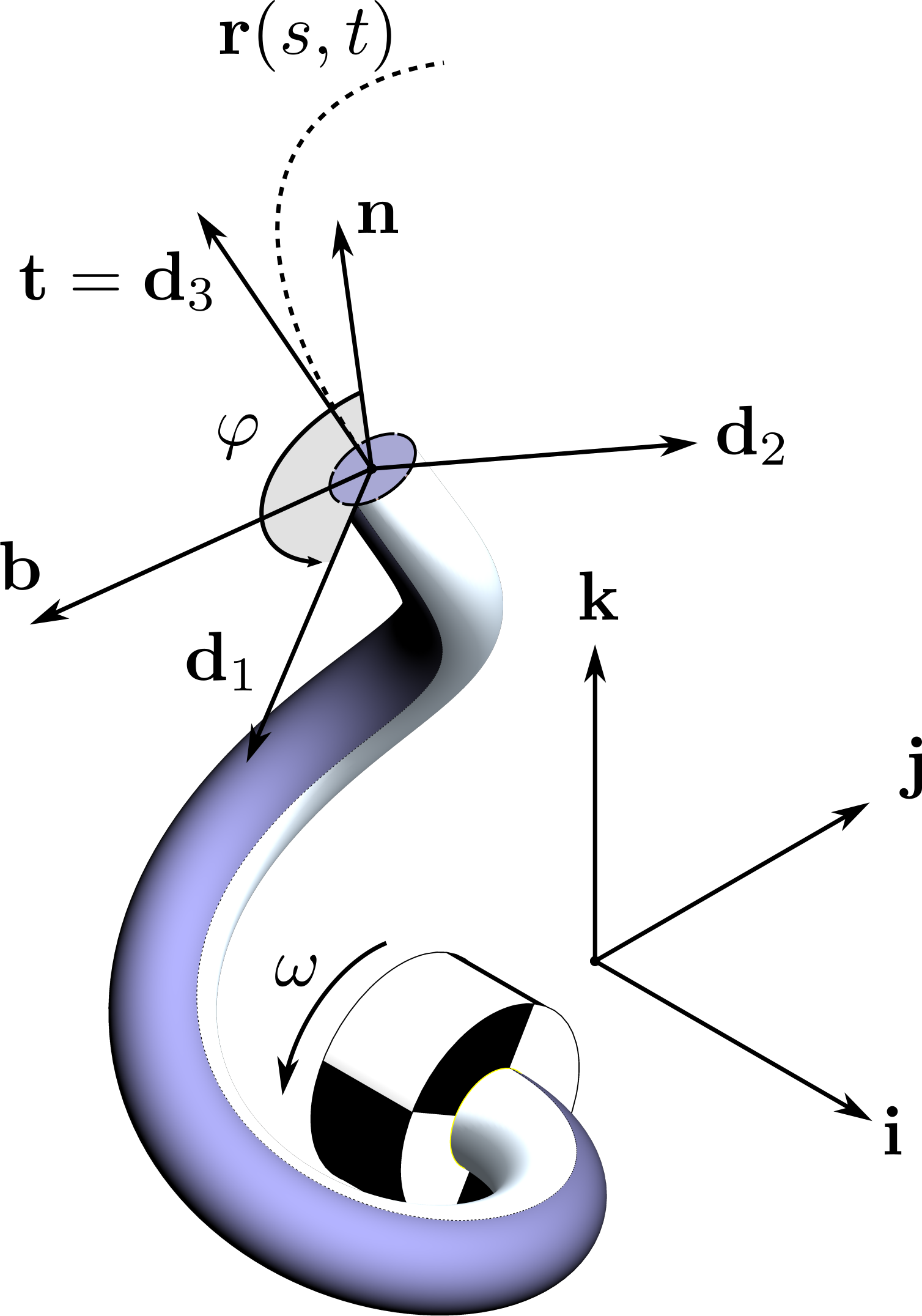
Figure 2: We model the shoot as a rod with centerline $\mathbf{r}$ and tangent $\mathbf{t}=\mathbf{d}_{3}$. At a given point at arclength $s$ from the base, the vectors $\mathbf{d}_{1}$ and $\mathbf{d}_{2}$ lie in the principal directions of the cross-section. At the base of the rod, $\mathbf{d}_{1}$ and $\mathbf{d}_{2}$ are rotating around $\mathbf{i}$ with angular speed $\omega$.

In gravitropism, gravisensing mechanisms activate pathways that result in differential growth of the cells [20, 21, 22, 23, 2, 24, 25, 16]. Changes in curvature then occur when cells on the bottom side of the shoot extend faster than those on the upper side [1, 26, 23]. Assuming local growth laws for both gravitropism and autotropism leads, through dimensional reduction [27, 1], to a generalization of the sine law that includes autotropism and three-dimensional effects (Appendix A):

$$\mathbf{\dot{u}}+\mathbf{u}\times\mathbf{w}=\alpha\,\mathbf{t}\times\mathbf{k}-\beta\,\mathbf{u}.$$ (5)

Here, $\mathbf{u}\times\mathbf{w}$ accounts for the passive advection of $\mathbf{u}$ by the spin vector $\mathbf{w}$. The first term in the r.h.s accounts for gravitropism with rate constant $\alpha$. The second term models autotropism, with rate constant $\beta$, and leads to an exponential decay in time of the curvature in the absence of other effects. This equation reduces to the sine law in the planar case when $\beta=0$ and no rotation is imposed. The relative strength of gravitropism and autotropism is captured by the dimensionless bending number $\lambda\vcentcolon=\alpha\ell/\beta$ [9, 14]. Moreover, given the constitutive hypothesis that the local growth of the cells is parallel to the axis, we have [27]

$$\mathbf{u}\cdot\mathbf{t}=0.$$ (6)

The evolution of the tangent vector along the shoot is given by Eq. 3:

$$\mathbf{t}^{\prime}=\mathbf{u}\times\mathbf{t}.$$ (7)

Eqs. 4, 5, 7 and 6 form a closed system for $\mathbf{u}$, $\mathbf{w}$ and $\mathbf{t}$ which, given appropriate initial and boundary conditions, fully captures the shape and evolution of the shoot. For comparison, our model is the three-dimensional, nonlinear generalization of the standard ‘AC model’, which has been validated experimentally in numerous genera [9]. In particular, our approach is general enough to include complex movements such as clinostatting, enforced through a non-zero spin $\mathbf{w}({0,t})\neq\mathbf{0}$ at the base.

Equilibria. –

We start our analysis by looking for equilibrium solutions in the absence of rotation, but for an arbitrary orientation of the base $\theta_{0}$ (Section B.1). In that case, the equilibrium solution is planar with the exact solution ${\tilde{z}\lambda}/{\ell}=\log(\sin\theta_{0})-\log(\sin(\theta_{0}-{\tilde{x}\lambda}/{\ell}))$, for $0\leq{\tilde{x}\lambda}/{\ell}<\theta_{0}$, with the tilde denoting quantities at equilibrium. We will establish that this solution is stable and gives the asymptotic shape of the shoot centerline when the base is tilted to an angle $\theta_{0}$ from the vertical, as shown in Fig. 3(a). On rescaling all lengths by the auto-gravitropic length $\ell_{\text{ag}}\vcentcolon=\ell/\lambda$, we obtain a universal curve [see Fig. 3(b)]:

$$\tilde{z}\!=\!\log(\sin\theta_{0})\!-\!\log(\sin(\theta_{0}\!-\!\tilde{x})),\ \quad 0\leq\tilde{x}<\theta_{0}.$$ (8)

We refer to this curve as the simple caulinoid (from Latin caulis, meaning stem).

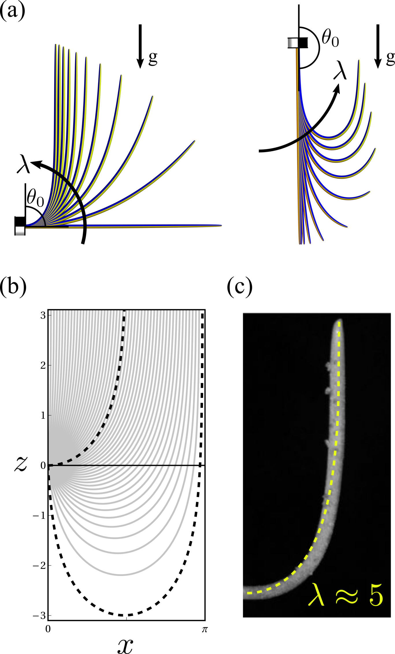
Figure 3: Steady solutions in the absence of clinostatting. (a) Horizontal clamp $\absolutevalue{\theta_{0}}=\pi/2$ and upside-down clamp $\absolutevalue{\theta_{0}}\rightarrow\pi^{-}$ for various $\lambda$. (b) The equilibrium solution is a simple caulinoid [Eq. 8] parameterized by $\theta_{0}$. Dashed lines show the horizontal and upside-down solutions. (c) Shape adopted by a wheat coleoptile (adapted from [9], with courtesy from B. Moulia) with overlaid caulinoid.

Next, we consider a clinostat imparting a counterclockwise rotation around the horizontal axis $\mathbf{i}$ with period $T=2\pi/\omega$. In this case, the boundary conditions are $\mathbf{t}({0,t})=\mathbf{i}$ and $\mathbf{w}({0,t})=\omega\mathbf{i}$. By definition, at equilibrium, we have $\mathbf{\dot{w}}=\mathbf{\dot{u}}=\mathbf{\dot{t}}=\mathbf{0}$, which gives $\mathbf{w}=\omega\mathbf{t}$. In this configuration, the shoot revolves at constant angular velocity $\omega$ about a fixed centerline [Fig. 3(a)] with tangent vector given by (Section B.2)

$$\mathbf{\tilde{t}}({s})= \frac{\cos\Lambda s}{\cosh\Theta s}\,\mathbf{i}-\frac{\sin\Lambda s}{\cosh\Theta s}\,\mathbf{j}+\tanh(\Theta s)\,\mathbf{k},$$ (9)

where $\Lambda\vcentcolon={\alpha\omega}/({\omega^{2}+\beta^{2}})$ and $\Theta\vcentcolon={\alpha\beta}/({\omega^{2}+\beta^{2}})$. The curvature, $\tilde{\kappa}({s})=\sqrt{\Theta^{2}+\Lambda^{2}}\,\sech\Theta s$, and torsion, $\tilde{\tau}({s})=-\Lambda\tanh\Theta s$, of this general caulinoid satisfy

$$\frac{\tilde{\kappa}^{2}}{\Theta^{2}+\Lambda^{2}}+\frac{\tilde{\tau}^{2}}{\Lambda^{2}}=1.$$ (10)

Thus, along an equilibrium solution, starting from $\tilde{\tau}({0})=0$ at the base, the torsion increases while the curvature decreases along an ellipse in the curvature-torsion plane. In physical space, the centerline follows a modulated left-handed helix that gradually uncoils away from the base towards the vertical, and we can interpret $\Lambda$ and $\Theta$ as the curve’s winding and rise densities [Fig. 4(b)]. In the limit $\omega\rightarrow 0$, we have $\Lambda=0$ and $\Theta=1/\ell_{\text{ag}}$, recovering the planar case discussed above. When $\omega\rightarrow\infty$, the plant remains straight with $\Lambda=\Theta=0$ [Fig. 4(c)]. The equilibrium curve is uniquely determined by $\Lambda$ and $\Theta$. Experimentally, given $\omega$, both parameters $\alpha$ and $\beta$ can thus be estimated uniquely from the centerline (unlike in the planar case), e.g. by using the height of the plant $H=\tilde{z}(1)=\log({\cosh\Theta})/\Theta$ and the radius of the caulinoid at the base $R=1/\Lambda$.

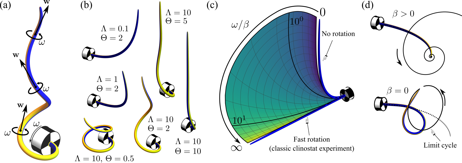
Figure 4: Dynamic equilibrium of a rotating plant. (a) The material revolves at angular speed $\omega$ around a fixed centerline. (b) Example equilibrium configurations obtained for various values of $\Lambda$ and $\Theta$. (c) Dependency of the equilibrium solution on $\omega$. Blue rods show the limits $\omega\rightarrow 0$ (no rotation) and $\omega\rightarrow\infty$ (standard clinostat experiment). The surface shows the set of equilibrium solutions obtained for finite values of $\omega/\beta$ ($\lambda=5$). (d) Course of the apex in two cases, $\beta>0$, with convergence to equilibrium ($\beta=\omega/5$), and $\beta=0$, after convergence to a limit cycle (in both cases $\alpha=\omega$). Dashed line shows the corresponding equilibrium solution.

A numerical linear stability analysis of the full system (Appendix D) conducted across a wide range of realistic parameters $\lambda\in\left[0.1,100\right]$ [Fig. 3(c)], consistent with reported values [9, 14, 28], reveals that, for $\beta>0$, the equilibrium solution is linearly stable. Further, the local dynamics near the base can be obtained asymptotically, showing that the Darboux vector spirals towards its equilibrium value with a typical exponential decay ${\text{e}}^{-\beta t}$ [see Fig. 4(d) and Movie 1]. In the limit case $\beta=0$ but with $\omega\not=0$ [1], the equilibrium solution is a segment of a horizontal circle of radius $\omega/\alpha$. Here, however, the previous stability result does not apply and the shoot orbits around the equilibrium [see Fig. 4(d) and Movie 2].

Shoot elongation. –

Plants also lengthen due to the coordinated expansion of the cells along the central axis. Generally, this primary growth is mostly confined to a region close to the apex [29]. To model elongation, including apical dominance, we assume that both the tropic response and axial growth gradually diminish as we move away from the apex with exponential decay of characteristic length $\delta$ and with growth $\Gamma_{0}$ and auto-gravitropic rates, $\beta$ and $\alpha$, at the tip (Appendix E). In this case, the system supports a traveling front solution connecting a flat base to a steady apical structure migrating forward at a speed $c=\Gamma_{0}\delta$ [see Fig. 5(a) and Movie 3]. The shape of this solitary wave can be described in terms of an initial value problem that can be integrated numerically. Fig. 5(b) shows example solutions obtained for various rotation speeds and bending numbers $\lambda$. An interesting limit is $\ell\ll\delta$ (uniform growth rates along the shoot). Assuming a timescale separation $\beta\gg\Gamma_{0}$, and noting that $\Lambda$ and $\Theta$ are independent of $\ell$, we see that the shoot’s shape will progress quasi-statically, spreading itself uniformly along a unique caulinoid [see Fig. 5(d) and Movie 4]. The existence of these solutions demonstrates that steady configurations are a robust property of the system that can persist even upon significant elongation.

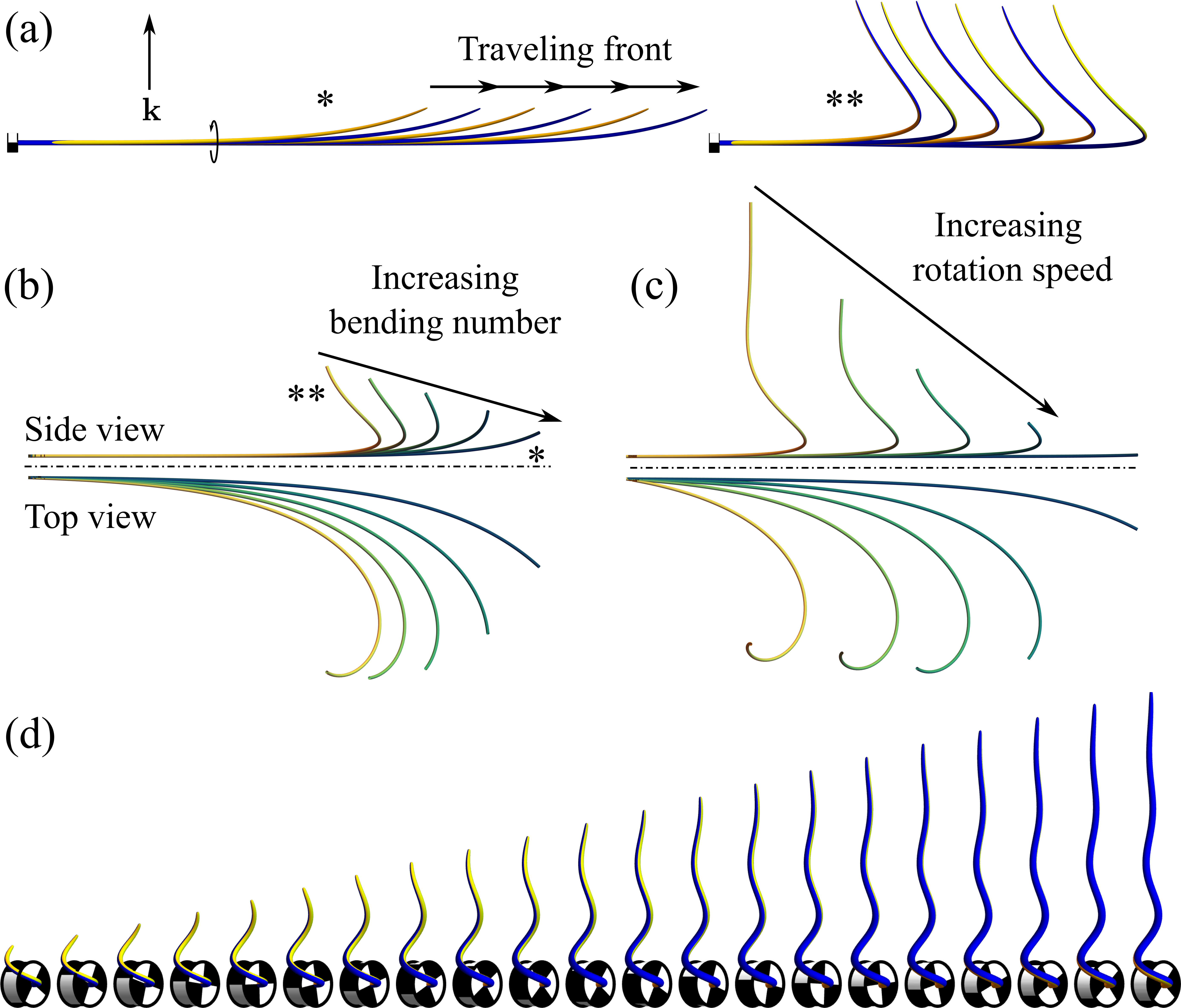
Figure 5: Growth. (a) Examples of simulated growing shoots (parameters: $\alpha=\omega$ and $5\omega$; $\beta=\omega$; $\delta=\ell$; $\Gamma_{0}=\omega/10$). (b, c) Solitary wave profiles computed for different (b) bending numbers $\lambda$; and (c) rotation speeds $\omega$. The labels $*$ and $**$ indicate corresponding sets of parameters between the simulation and the asymptotic profile. (d) Uniform growth rate ($\delta\gg\ell$): The plant spreads along a unique caulinoid (here, $\Lambda=5$, $\Theta=1$, $\Gamma_{0}=\omega/10$).

Discussion. –

The clinostat holds a significant place in plant physics, addressing a precise technical challenge: simulating weightlessness by effectively ‘confusing’ the plant through fast rotation. At lower speeds, the interaction between rotation, gravitropism, and autotropism reveals more subtle behaviors. A distinct property of this system is the universal existence of a dynamic equilibrium where the shoot revolves around a steady centerline, the caulinoid. This equilibrium is dynamic as it requires cyclic deformations in the material to maintain this configuration as rotation is applied. In contrast to the classic planar case, whose equilibrium is determined solely by $\lambda$ (Fig. 3), this solution is uniquely characterized through two dimensionless numbers $\alpha\ell/\omega$ and $\beta/\omega$. When the plant undergoes elongation, two distinct behaviors emerge: solitary waves when growth, autotropism and gravitropism are confined to the tip; or stationary elongation along a unique caulinoid when the shoot grows uniformly. In conclusion, we predict that a clinostatting shoot will naturally assume the sole shape that enables it to counterbalance rotation and minimize its overall movement in the laboratory frame, strikingly, even in the absence of a dedicated rotation-sensing mechanism.

The importance of proprioception in plant posture control is now well established [9, 3, 2, 30, 31, 31, 16]. We further showed that the role of proprioception, in the form of autotropism, is crucial in stabilizing the clinostatting shoot, as its absence would lead to non-steady behaviors [1]. Physically, autotropism acts as a damping mechanism in curvature space, hence providing a stabilization mechanism. The exact caulinoid solutions may be difficult to observe experimentally with precision as it would require pristine conditions. Further, in plants, heterogeneity, stochasticity and other tropic responses also play a role. Yet, these ideal solutions present a new paradigm for the study of plant shapes and the design of experiments. They can be further generalized to include other effects, such as light, or elasticity [1]. They demonstrate that the coupling of internal and external stimuli is key for shape control, a problem of general importance in biology with direct implications for non-living active materials.

A.G. acknowledges support from the Engineering and Physical Sciences Research Council of Great Britain under Research Grant No. EP/R020205/1. H.A.H. acknowledges support from the Royal Society under University Research Fellowship No. URF/R/211032. For the purpose of Open Access, the author has applied a CC BY public copyright license to any Author Accepted Manuscript (AAM) version arising from this submission.

Appendix A Kinetics of curvature evolution

The auto-gravitropic governing law, derived in [1], reads in vector form:

$$\boldsymbol{\dot{\sf u}}=\alpha\boldsymbol{\sf t}\times\boldsymbol{\sf k}-\beta\boldsymbol{\sf u}.$$ (11)

Here, we have used Antman’s sans-serif notations [32] to denote vector field attached to a curve and expressed in the local material frame $\mathbf{d}_{i}$, i.e. for a vector field $\mathbf{u}({s,t})$, we write

$$\mathbf{u}({s,t})=\sum_{i=1}^{3}{\sf u}_{i}({s,t})\mathbf{d}_{i}({s,t}),$$ (12)

and $\boldsymbol{\sf u}=({{\sf u}_{1},{\sf u}_{2},{\sf u}_{3}})$ then denotes the vector of local coordinates ${\sf u}_{i}=\mathbf{u}\cdot\mathbf{d}_{i}$ (in particular, $\mathbf{t}=\mathbf{d}_{3}$ implies $\boldsymbol{\sf t}=({0,0,1})$). Thus, Eq. 11 expresses the evolution of curvatures from a local point of view, i.e. in a reference frame attached to the material. In our case, since gravity is important, it is convenient to express the dynamics in the non-rotating, laboratory frame (indeed, the equilibrium solutions are naturally expressed in the laboratory frame). Therefore, we differentiate Eq. 12 with respect to time, and use $\mathbf{\dot{d}}_{i}=\mathbf{w}\times\mathbf{d}_{i}$ [Eq. 3], to obtain the kinematic relation

$$\mathbf{\dot{u}}+\mathbf{u}\times\mathbf{w}=\sum_{i=1}^{3}\dot{\sf u}_{i}\mathbf{d}_{i}.$$ (13)

Using the rotational invariance of the cross product, Eqs. 11 and 13 directly provide the expression given in Eq. 5 for $\mathbf{\dot{u}}$.

Appendix B Equilibrium solutions

B.1 Without rotation

We derive the equilibrium solutions for the non-rotating case ($\omega=0$). Here, we choose $\ell\equiv 1$ as a reference length unit. Setting $\mathbf{\dot{u}}=\mathbf{0}$ in Eq. 5 provides $\mathbf{\tilde{u}}=\lambda\mathbf{\tilde{t}}\times\mathbf{k}$, which can be substituted into Eq. 7 to obtain

$$\mathbf{\tilde{t}}^{\prime}=\lambda({\mathbf{\tilde{t}}\times\mathbf{k}})\times\mathbf{\tilde{t}}.$$ (14)

Provided an initial tilt $0\leq\theta_{0}<\pi$, such that $\mathbf{\tilde{t}}({0})=\sin\theta_{0}\,\mathbf{i}+\cos\theta_{0}\,\mathbf{k}$, we integrate this equation and derive the tangent

$$\mathbf{\tilde{t}}({s}) =\frac{\sin\theta_{0}}{\cos\theta_{0}\sinh\lambda s+\cosh\lambda s}\,\mathbf{i}$$

$$+{\frac{(\cos\theta_{0}+1){\text{e}}^{2\lambda s}-1+\cos\theta_{0}}{(\cos\theta_{0}+1){\text{e}}^{2\lambda s}+1-\cos\theta_{0}}}\,\mathbf{k}.$$ (15)

Integrating once more gives the position vector $\mathbf{\tilde{r}}({s})=\tilde{x}({s})\,\mathbf{i}+\tilde{z}({s})\,\mathbf{k}$:

$$\lambda\tilde{x}({s})={\theta_{0}-2\arccot\left({\text{e}}^{\lambda s}\cot\frac{\theta_{0}}{2}\right)},$$ (16a)

$$\lambda\tilde{z}({s})=\log\left[1+\cos^{2}({{\theta_{0}}/{2}})({{\text{e}}^{2\lambda s}-1})\right]-\lambda s.$$ (16b)

Inverting Eq. 16a and rescaling all lengths as $\tilde{x}\rightarrow\tilde{x}/\lambda$, $\tilde{z}\rightarrow\tilde{z}/\lambda$, we obtain an implicit relation between $\tilde{z}$ and $\tilde{x}$ [Eq. 8], which corresponds to a universal equilibrium shape for all orientations $\theta_{0}$ of the shoot.

B.2 With rotation

Next, we derive the equilibrium solution for a plant undergoing rotation ($\omega>0$). To determine the equilibrium shape, we posit $\mathbf{\dot{w}}=\mathbf{\dot{t}}=\mathbf{\dot{u}}=\mathbf{0}$. Eqs. 3 and 4 directly provide that $\mathbf{\tilde{w}}=\omega\mathbf{\tilde{t}}$. Substituting this ansatz into Eq. 5, we obtain

$$\beta\mathbf{\tilde{u}}=\mathbf{\tilde{t}}\times({\alpha\mathbf{k}+\omega\mathbf{\tilde{u}}}).$$ (17)

On inverting this identity, we can express $\mathbf{\tilde{u}}$ as an explicit function of $\mathbf{\tilde{t}}$, given by

$$\mathbf{\tilde{u}}=({\Lambda\tilde{t}_{1}\tilde{t}_{3}+\Theta\tilde{t}_{2}})\,\mathbf{i} +({\Lambda\tilde{t}_{2}\tilde{t}_{3}-\Theta\tilde{t}_{1}})\,\mathbf{j}$$

$$+\Lambda({\tilde{t}_{3}^{2}-1})\,\mathbf{k},$$ (18)

with $\mathbf{\tilde{t}}=\tilde{t}_{1}\,\mathbf{i}+\tilde{t}_{2}\,\mathbf{j}+\tilde{t}_{3}\,\mathbf{k}$. Substituting this last expression into Eq. 7 and integrating it, we obtain the expression for the tangent given by Eq. 9. Remarkably, we can integrate the tangent to obtain an exact parameterization of the centerline $\mathbf{\tilde{r}}$, in terms of the hypergeometric function ${}_{2}F_{1}$, the harmonic number $H_{n}$ and the polygamma function of order zero $\psi^{(0)}$:

$$\tilde{x}({s}) =\frac{{\text{e}}^{s(\Theta+{\text{i}}\Lambda)}}{\Theta+{\text{i}}\Lambda}\,_{2}F_{1}\left(1,\frac{\Theta+{\text{i}}\Lambda}{2\Theta};\frac{3\Theta+{\text{i}}\Lambda}{2\Theta};-{\text{e}}^{2s\Theta}\right)+\frac{{\text{e}}^{s(\Theta-{\text{i}}\Lambda)}\,}{\Theta-{\text{i}}\Lambda}\,_{2}F_{1}\left(1,\frac{\Theta-{\text{i}}\Lambda}{2\Theta};\frac{3\Theta-{\text{i}}\Lambda}{2\Theta};-{\text{e}}^{2s\Theta}\right)$$

$$-\frac{\pi}{2\Theta}\sech\left(\frac{\pi\Lambda}{2\Theta}\right),$$ (19a)

$$\tilde{y}({s}) =\frac{{\text{i}}}{4\Theta}\left[\psi^{(0)}\left(\frac{\Theta+{\text{i}}\Lambda}{4\Theta}\right)-\psi^{(0)}\left(\frac{3\Theta+{\text{i}}\Lambda}{4\Theta}\right)+H_{-\frac{\Theta+{\text{i}}\Lambda}{4\Theta}}-H_{-\frac{3\Theta+{\text{i}}\Lambda}{4\Theta}}\right]$$

$$+\frac{{\text{e}}^{s(\Theta+{\text{i}}\Lambda)}}{\Lambda-{\text{i}}\Theta}\,_{2}F_{1}\left(1,\frac{\Theta+{\text{i}}\Lambda}{2\Theta};\frac{3\Theta+{\text{i}}\Lambda}{2\Theta};-{\text{e}}^{2s\Theta}\right)+\frac{{\text{e}}^{s(\Theta-{\text{i}}\Lambda)}}{\Lambda+{\text{i}}\Theta}\,_{2}F_{1}\left(1,\frac{\Theta-{\text{i}}\Lambda}{2\Theta};\frac{3\Theta-{\text{i}}\Lambda}{2\Theta};-{\text{e}}^{2s\Theta}\right),$$ (19b)

$$\tilde{z}({s}) =\frac{\log(\cosh(\Theta s))}{\Theta}.$$ (19c)

Fig. 6 shows the set of solution shapes for different values of $\Lambda$ and $\Theta$. Inset shows the path of the solution in the $\kappa$-$\tau$ space, which follows the ellipse given by Eq. 10.

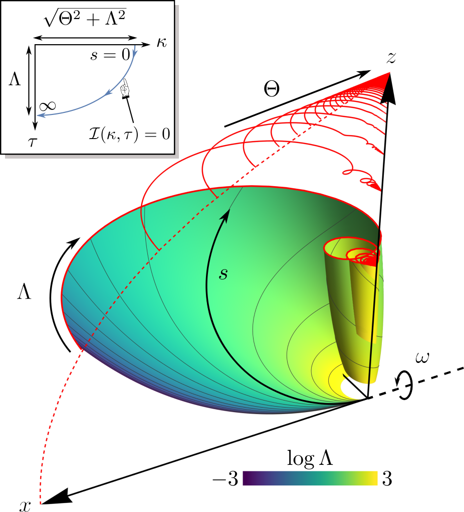
Figure 6: Set of equilibrium solutions. The colored surface plot sweeps solutions for a range of $\Lambda$ (with $\Theta=1$). Red solid lines show the course of the shoot tip $s=0$ as $\Lambda$ varies, and for different values of $\Theta>1$, with height given by $h({\Theta})=\log(\cosh\Theta)/\Theta$. Red dashed line shows the tip position for $\Lambda=0$ as a function of $\Theta$, given by $({x({\Theta}),z({\Theta})})=({\operatorname{gd}\Theta/\Theta,h({\Theta})})$. Inset shows the path of the solution in the $\kappa$–$\tau$ plane [Eq. 10].

Appendix C Numerical resolution of the nonlinear system

We use a method based on Chebyshev polynomials to integrate numerically the nonlinear system given by Eqs. 5, 7, 4 and 6. We first remark that the system, albeit originally defined for $s\in\left[0,1\right]$, can be extended naturally to $s\in\left[-1,1\right]$ (by considering two ‘twin’ shoots oriented opposite to each other with respect to the plane $y$-$z$). Here, the extended equilibrium solution is invariant with respect to the mirror symmetry $x\rightarrow-x$, $s\rightarrow-s$. This situation is ideal for using Chebyshev polynomials of the first kind $T_{n}$ [33] as they are defined canonically on $\left[-1,1\right]$. Thus, we consider the truncated Chebyshev expansions for the variables

$$\mathbf{t}\approx\sum_{n=0}^{N}\mathbf{T}^{n}T_{n},$$ (20a)

$$\mathbf{w}\approx\sum_{n=0}^{N}\mathbf{W}^{n}T_{n},$$ (20b)

$$\mathbf{u}\approx\sum_{n=0}^{N}\mathbf{U}^{n}T_{n},$$ (20c)

with $N$ a positive integer.

The formal solutions for $\mathbf{t}$ and $\mathbf{w}$,

$$\mathbf{t}=\mathbf{i}+\int_{0}^{s}\mathbf{u}\times\mathbf{t},$$ (21a)

$$\mathbf{w}=\omega\mathbf{i}+\alpha\int_{0}^{s}\mathbf{t}\times\mathbf{k}-\beta\int_{0}^{s}\mathbf{u},$$ (21b)

can be decomposed on the Chebyshev basis as follows. From the products $T_{n}T_{m}=({T_{n+m}+T_{\absolutevalue{n-m}}})/2$ [33], we derive the expansion of the cross products, i.e., for any vector field $\mathbf{a}$ and $\mathbf{b}$ with respective Chebyshev coefficients $\mathbf{A}^{n}$ and $\mathbf{B}^{n}$, we have

$$\mathbf{a}\times\mathbf{b}=\frac{1}{2}\sum_{p=0}^{\infty}({\mathbf{A}^{p}\times\mathbf{B}^{p}+\mathbf{A}^{p}\times\mathbf{B}^{-p}})T_{0}+\frac{1}{2}\sum_{n=1}^{\infty}\sum_{p=0}^{n}({\mathbf{A}^{p}\times\mathbf{B}^{n-p}+\mathbf{A}^{p}\times\mathbf{B}^{n+p}+\mathbf{A}^{n+p}\times\mathbf{B}^{p}})T_{n}.$$ (22)

For integration, we use the recurrence formulae [33]

$$\int T_{0}=T_{1};\quad\int T_{1}=\frac{1}{4}({T_{2}+T_{0}});$$ (23a)

$$\int T_{n}=\frac{1}{2}({\frac{T_{n+1}}{n+1}-\frac{T_{n-1}}{n-1}}),\quad\forall n\geq 2,$$ (23b)

to obtain

$$\int\mathbf{a}=\frac{\mathbf{A}^{1}}{4}T_{0}+\mathbf{A}^{0}T_{1}+\sum_{n=2}^{\infty}\frac{\mathbf{A}^{n-1}-\mathbf{A}^{n+1}}{2n}T_{n}.$$ (24)

Conveniently, integration corresponds to a linear operation on the $\mathbf{A}^{n}$, whose matrix can be precomputed.

Given the coefficients $\mathbf{U}^{n}$, the Chebyshev expansion of Eq. 21a yields a linear system that can be inverted to obtain the $\mathbf{T}^{n}$. Then, the $\mathbf{W}^{n}$ are obtained by direct integration, using Eq. 24. After expressing the $\mathbf{T}^{n}$ and $\mathbf{W}^{n}$ as functions of the $\mathbf{U}^{n}$, we obtain a dynamical system of the form

$${\dot{\mathbb{U}}}=\mathcal{F}({{\mathbb{U}}}),$$ (25)

where ${\mathbb{U}}$ is the $3({N+1})$-dimensional vector formed by the concatenation of the $\mathbf{U}^{n}$; and $\mathcal{F}$ is a second-degree polynomial vector that is evaluated numerically. Provided appropriate initial conditions, Eq. 25 can be integrated numerically using a standard IVP solver (here we used Mathematica’s built-in routine NDSolve).

A general problem is to find an initial condition for $\mathbf{u}$ that satisfies the orthogonality condition, Eq. 6. Indeed, by differentiating $\mathbf{u}\cdot\mathbf{t}$ with respect to time and using Eq. 5, we observe that

$$\frac{\partial{}}{\partial{t}}({\mathbf{u}\cdot\mathbf{t}})=-\beta\mathbf{u}\cdot\mathbf{t}.$$ (26)

Since $\beta>0$, Eq. 6 is a stable property, in particular, if Eq. 6 is satisfied at $t=0$, it will be automatically satisfied at all times $t$. Note that, if $\mathbf{u}\cdot\mathbf{t}=0$, then we have automatically

$$\mathbf{u}=\mathbf{t}\times\mathbf{t}^{\prime}$$ (27)

(the converse is trivial). Thus a suitable initial condition can always be found by first defining a curve and its tangent $\mathbf{t}$; and then obtaining $\mathbf{u}$ through Eq. 27. Once an initial configuration is defined, the initial Chebyshev coefficients for $\mathbb{U}({0})$ are computed efficiently by means of the discrete cosine transform [34].

Appendix D Stability

D.1 Asymptotic analysis near the base

To gain insight into the dynamics of the shoot and its stability, it is useful to first restrict our attention to the base of the plant, $s=0$, where $\mathbf{t}({0,t})=\mathbf{i}$ and $\mathbf{w}({0,t})=\omega\mathbf{i}$. Letting $\mathbf{U}({t})=\mathbf{u}({0,t})$, Eq. 5 reduces to

$$\dot{U}_{2}=-\alpha-\beta U_{2}-\omega U_{3},\quad\dot{U}_{3}=\omega U_{2}-\beta U_{3}.$$ (28)

with $\mathbf{U}=U_{2}\,\mathbf{j}+U_{3}\,\mathbf{k}$. We have $U_{1}=0$ by Eq. 6. The system admits a unique fixed point $({U_{2},U_{3}})=({-\Theta,-\Lambda})$ (this is simply the equilibrium curvatures at the origin derived in Section B.2), associated with a pair of conjugate eigenvalues $-\beta\pm\omega{\text{i}}$ with negative real part: The fixed point is a spiral sink associated with a decaying amplitude $\sim{\text{e}}^{-\beta t}$ and rotation speed $\omega$. When $\beta=0$ the fixed point is a center and the solution orbits around the fixed point.

We can extend this analysis to higher orders in $s>0$ in principle (that is, expanding all variables in orders of $s$ and performing a regular perturbation). For instance, Fig. 7 shows the second-order approximation of the solution taken at $s=0.25$. The second-order estimate converges towards equilibrium when $\beta>0$ and $s\ll 1$ (in the case $\beta=0$ however, there is a secular term that must be treated by a dedicated method, but we leave this problem outside the scope of this study, focusing on the physiologically relevant case $\beta>0$).

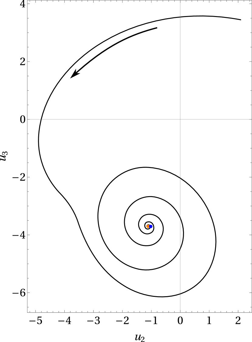
Figure 7: Example course of the Darboux vector $\mathbf{u}({t})$ in the plane $\mathbf{j}$-$\mathbf{k}$, computed asymptotically (to second order in $s$) near the base ($s=0.25$). The asymptotic solution spirals towards an equilibrium value ($\alpha=4\omega$, $\beta=0.2\omega$). Blue and orange dots show the exact value of $\mathbf{u}$ at equilibrium at $s$, and its second-order approximation, respectively.

D.2 Linear stability analysis

The previous analysis provides insight into the dynamics of the system; however, in principle, it is valid only near the base. To complement that approach, we perform a linear stability analysis of the equilibrium solution. Therefore, we take the first variation of Eqs. 5, 4, 7 and 6 around the base equilibrium solution derived in Section B.2. Rearranging the terms, we obtain:

$$\delta\mathbf{t}^{\prime}=\delta\mathbf{u}\times\mathbf{\tilde{t}}+\mathbf{\tilde{u}}\times\delta\mathbf{t},$$ (29a)

$$\delta\mathbf{w}^{\prime}=\alpha\,\delta\mathbf{t}\times\mathbf{k}-\beta\delta\mathbf{u},$$ (29b)

$$\delta\mathbf{\dot{u}}=\delta\mathbf{w}^{\prime}+\delta\mathbf{w}\times\mathbf{\tilde{u}}+\mathbf{\tilde{w}}\times\delta\mathbf{u},$$ (29c)

with the conditions

$$\mathbf{\tilde{u}}\cdot\delta\mathbf{t}=-\delta\mathbf{u}\cdot\mathbf{\tilde{t}},\quad\mathbf{\tilde{t}}\cdot\delta\mathbf{t}=0.$$ (30)

The boundary conditions at $s=0$ fix the values of $\mathbf{t}({0,t})$ and $\mathbf{w}({0,t})$, thus,

$$\delta\mathbf{t}({0,t})=\mathbf{0},\quad\delta\mathbf{w}({0,t})=\mathbf{0}.$$ (31)

We start by solving Eq. 29a. As can be seen, a linearly independent basis of solutions for the homogeneous part of Eq. 29a is provided by the $\mathbf{d}_{i}$ at equilibrium (defined up to an arbitrary rotation of the clinostat). A particular solution is then obtained by means of variation of constants. For a given $\delta\mathbf{u}$, the solutions to Eqs. 29a, 29b and 31 are:

$$\delta\mathbf{t}=\mathbf{d}_{1}\int_{0}^{s}\delta{\mathbf{u}}\cdot\mathbf{d}_{2}-\mathbf{d}_{2}\int_{0}^{s}\delta{\mathbf{u}}\cdot\mathbf{d}_{1},$$ (32a)

$$\delta\mathbf{w}=-\alpha\mathbf{k}\times\int_{0}^{s}\delta\mathbf{t}-\beta\int_{0}^{s}\delta\mathbf{u}.$$ (32b)

Lastly, we perform a Chebyshev spectral analysis of the linearized system. Namely, expanding Eqs. 32 and 29c as in Appendix C, we obtain a linear dynamical system

$$\delta\dot{\mathbb{U}}=\mathbf{L}\delta\mathbb{U}$$ (33)

for the Chebyshev coefficients $\delta\mathbb{U}$. Note that, since the orthogonality constraint, Eq. 30, is stable by Eq. 26, we need not consider it in the stability analysis, as coordinates orthogonal to the constraint surface will vanish. The complex eigenvalues of $\mathbf{L}$ can be computed numerically; specifically, the system is linearly stable if all the real parts $\omega_{i}\in\mathbb{R}^{3({N+1})}$ of these eigenvalues are negative. Here, the system appears to be stable for all values of $\lambda$ and $\omega$ tested. The results are consistent with the dynamics predicted in Section D.1, which is dominated by a decay rate of order ${\text{e}}^{-\beta t}$.

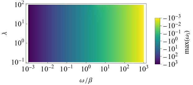
Figure 8: Numerical linear stability analysis. Density plot showing the value of the largest real part $\omega_{i}$ of the eigenvalues of Eq. 33 (to generate this plot, the system was re-expressed in terms of the dimensionless time $\omega t$). This shows that the dynamics is dominated by a decay rate of order ${\text{e}}^{-\beta t}$ as expected from Section D.1.

Appendix E Shoot elongation

E.1 General model

To model growth, we introduce the standard growth multiplier $\gamma\vcentcolon={\partial{s}}/{\partial{s_{0}}}$ which connects the arclength $s_{0}\in\left[0,\ell_{0}\right]$ in the initial configuration of the shoot, to the arclength $s\in\left[0,\ell({t})\right]$ in the current, grown configuration [19]. To account for apical dominance, we assume that growth and curvature generation mostly happen within a finite distal section of the stem of length $\delta$. Therefore, we introduce an activation function:

$$a({s_{0},t})=f({\ell({t})-s({s_{0},t})}),$$ (34)

with $f({\sigma})={\text{e}}^{-\sigma/\delta}$, modeling the slowing down of growths as we move away from the tip of the shoot, located at $\ell({t})=s({\ell_{0},t})$. Accordingly, we assume an exponential growth kinetics given by [19]

$$\Gamma\vcentcolon=\frac{\dot{\gamma}}{\gamma}=\Gamma_{0}\,a({s_{0},t}),$$ (35)

which captures a type of growth where all cells in a small portion of the tissue expand and proliferate at the same rate. Similarly, we define the rates of curvature generation $A({s_{0},t})=\alpha a({s_{0},t})$, and $B({s_{0},t})=\beta a({s_{0},t})$. Note that the model can be easily adapted to include richer apical growth models, e.g. sigmoids [35], however, we do not expect any significant qualitative change in the results.

On integrating the standard kinematic relation ${\partial{\dot{s}}}/{\partial{s}}=\Gamma$ using Eqs. 35 and 34, we obtain

$$\dot{s}=c{\text{e}}^{-\ell/\delta}({{\text{e}}^{s/\delta}-1}),$$ (36)

with $c\vcentcolon=\Gamma_{0}\delta$ a characteristic speed; and where $\ell$ is governed by

$$\dot{\ell}=c\left(1-{\text{e}}^{-\ell/\delta}\right),$$ (37)

as a particular case of Eq. 36. Provided the initial condition $\ell({0})=\ell_{0}\equiv 1$, the previous equation integrates as

$$\ell({t})=\delta\log({({\text{e}}^{{1}/{\delta}}-1)\,{\text{e}}^{\Gamma_{0}t}+1}).$$ (38)

Integrating Eq. 36 with Eq. 38 then gives

$$s({s_{0},t})=\delta\log\left[\frac{1}{2}-\frac{1}{2}\tanh\left(\frac{\Gamma_{0}t}{2}+\frac{1}{2\delta}+\arctan(1-2{\text{e}}^{s_{0}/\delta})-\frac{1}{2}\log\left(({\text{e}}^{1/\delta}-1){\text{e}}^{\Gamma_{0}t}+1\right)\right)\right].$$ (39)

Thus,

$$f({s_{0},t})=\left[\exp({\frac{ct+1-s_{0}}{\delta}})-{\text{e}}^{\Gamma_{0}t}+1\right]^{-1},$$ (40)

and

$$\gamma({s_{0},t})=\left[\left(1-{\text{e}}^{\Gamma_{0}t}\right)\exp({\frac{s_{0}-ct-1}{\delta}})+1\right]^{-1}.$$ (41)

In the context of a growing spatial domain, one must differentiate between the material (Lagrangian) derivative, denoted with an overdot $\mathbf{\dot{u}}$, and the Eulerian derivative denoted ${\partial{\mathbf{u}}}/{\partial{t}}$, and such that

$$\mathbf{\dot{u}}=\frac{\partial{\mathbf{u}}}{\partial{t}}+\dot{s}\frac{\partial{\mathbf{u}}}{\partial{s}}.$$ (42)

The vectors $\mathbf{u}$ and $\mathbf{w}$ are defined here in the Eulerian sense, namely such that

$$\frac{\partial{\mathbf{t}}}{\partial{s}}=\mathbf{u}\times\mathbf{t},\quad\frac{\partial{\mathbf{t}}}{\partial{t}}=\mathbf{w}\times\mathbf{t},$$ (43)

with the compatibility condition

$$\frac{\partial{\mathbf{u}}}{\partial{t}}-\frac{\partial{\mathbf{w}}}{\partial{s}}=\mathbf{w}\times\mathbf{u}.$$ (44)

In contrast, the Lagrangian spin vector, $\mathbf{p}=\mathbf{w}+\dot{s}\mathbf{u}$, is associated with

$$\mathbf{\dot{t}}=\mathbf{p}\times\mathbf{t}.$$ (45)

The revised governing equations, including growth, are then

$$\mathbf{t}^{\prime}=\gamma\mathbf{u}\times\mathbf{t},$$ (46a)

$$\mathbf{p}^{\prime}=\gamma({A\mathbf{t}\times\mathbf{k}-B\mathbf{u}}),$$ (46b)

$$\mathbf{\dot{u}}+\mathbf{u}\times\mathbf{p}+\Gamma\mathbf{u}=\mathbf{p}^{\prime}/\gamma,$$ (46c)

where $(\ )^{\prime}$ denotes a derivative with respect to the Lagrangian coordinate $s_{0}$. The extra term $\Gamma\mathbf{u}$ accounts for the passive decrease of curvature due to axial stretch. The presence of the factor $\gamma$ simply results from the chain rule, as we have expressed the system with respect to $s_{0}$.

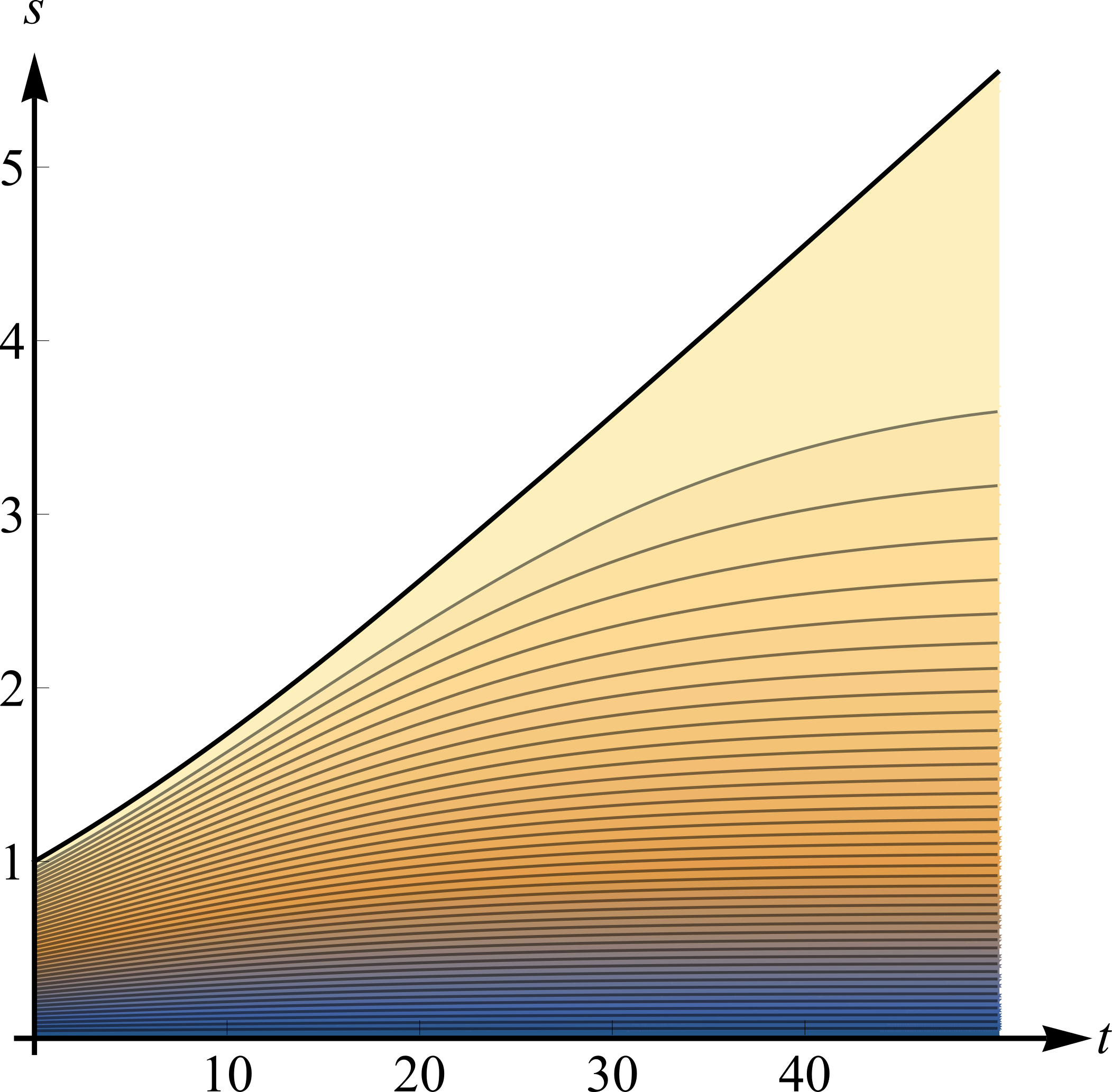
Figure 9: Kymograph showing the apical growth field. Lines show the trajectories of the material points with initial arclength emphasized by colors.

E.2 Solitary waves

To derive the shape of self-similar, traveling-front solutions we introduce the co-moving coordinate $\sigma\vcentcolon=\ell-s$, measuring the arclength from the apex, with the base located at $\sigma=\ell\rightarrow\infty$. Setting ${\partial{\mathbf{u}}}/{\partial{t}}=\mathbf{0}$, Eq. 46 becomes upon this change of coordinate:

$$\frac{\partial{\mathbf{t}}}{\partial{\sigma}}=\mathbf{t}\times\mathbf{u},$$ (47a)

$$\frac{\partial{\mathbf{p}}}{\partial{\sigma}}=f({\sigma})({\alpha\mathbf{k}\times\mathbf{t}+\beta\mathbf{u}}),$$ (47b)

$$cf({\sigma})\frac{\partial{\mathbf{u}}}{\partial{\sigma}}+\frac{\partial{\mathbf{p}}}{\partial{\sigma}}=\mathbf{p}\times\mathbf{u}-\Gamma\mathbf{u},$$ (47c)

with the conditions $\displaystyle\lim_{\sigma\rightarrow\infty}\mathbf{t}=\mathbf{i}$, $\displaystyle\lim_{\sigma\rightarrow\infty}\mathbf{p}=\omega\mathbf{i}$ and $\displaystyle\lim_{\sigma\rightarrow\infty}\mathbf{u}=\mathbf{0}$. In practice, the system can be integrated for $\sigma\in\left[0,\Sigma\right]$ with $\Sigma\gg\delta$, and with boundary conditions expressed at $\Sigma$. There is however a removable singularity at $\sigma\rightarrow\infty$, as $f({\sigma})$ is transcendentally small, which causes numerical difficulties in Eq. 47c. To alleviate this issue, we consider perturbed boundary conditions of the form $\mathbf{t}({\Sigma})=\mathbf{i}+\boldsymbol{\epsilon}_{t}({\Sigma})$, $\mathbf{p}({\Sigma})=\omega\mathbf{i}+\boldsymbol{\epsilon}_{p}({\Sigma}),$ and $\mathbf{u}({\Sigma})=\boldsymbol{\epsilon}_{u}({\Sigma})$, where $\boldsymbol{\epsilon}_{t}$, $\boldsymbol{\epsilon}_{p}$ and $\boldsymbol{\epsilon}_{u}$ denote small perturbations from the boundary conditions at $\sigma=\infty$. Expanding Eq. 47 and keeping only the higher order non-zero terms allows to solve for $\boldsymbol{\epsilon}_{t}$, $\boldsymbol{\epsilon}_{p}$ and $\boldsymbol{\epsilon}_{u}$, in order to express the perturbed boundary values [Fig. 5(b) is obtained with $\Sigma\approx 5\delta$].

Appendix F Code availability

All numerical methods were implemented in Wolfram Mathematica 13.0. Source code will be made publicly available upon acceptance of the manuscript for publication.

Appendix G Supplementary files

Movie 1. –

An example rotating shoot converging towards equilibrium [parameters as in Fig. 4(d), with $\beta=\omega/5$].

Movie 2. –

In the absence of autotropism, a shoot will orbit around a caulinoid [parameters as in Fig. 4(d), with $\beta=0$].

Movie 3. –

Example traveling solution [parameters as in Fig. 5(a), left-hand side simulation].

Movie 4. –

Uniform growth along a caulinoid [$\alpha=5\omega$, $\beta=\omega$, $\Gamma_{0}=\omega/10$, $\delta=100$].

References

- Moulton et al. [2020a] D. E. Moulton, H. Oliveri, and A. Goriely, Proceedings of the National Academy of Sciences 117, 32226 (2020a).
- Moulia et al. [2019] B. Moulia, R. Bastien, H. Chauvet-Thiry, and N. Leblanc-Fournier, Journal of Experimental Botany 70, 3467 (2019).
- Hamant and Moulia [2016] O. Hamant and B. Moulia, New Phytologist 212, 333 (2016).
- Moulia and Fournier [2009] B. Moulia and M. Fournier, Journal of experimental botany 60, 461 (2009).
- Johnsson [1971] A. Johnsson, Quarterly Reviews of Biophysics 4, 277 (1971).
- von Sachs [1882] J. von Sachs, Vorlesungen über Pflanzen-physiologie, Vol. 1 (W. Engelmann, 1882) Chap. 36.
- von Sachs [1879] J. von Sachs, Über orthotrope und plagiotrope Pflanzentheile, Arbeiten des botanischen Instituts in Würzburg, Vol. 2 (W. Engelmann, 1879) Chap. 10.
- Cook [1969] J. Cook, Mathematical Biosciences 5, 353 (1969).
- Bastien et al. [2013] R. Bastien, T. Bohr, B. Moulia, and S. Douady, Proceedings of the National Academy of Sciences 110, 755 (2013).
- Pfeffer [1904] W. F. P. Pfeffer, Pflanzenphysiologie: Ein Handbuch der Lehre vom Stoffwechsel und Kraftwechsel in der Pflanze. Kraftwechsel. II, Vol. 3 (W. Engelmann, 1904).
- Polyanin and Zaitsev [2003] A. D. Polyanin and V. F. Zaitsev, Handbook of nonlinear partial differential equations: exact solutions, methods, and problems (Chapman and Hall/CRC, 2003).
- Bastien et al. [2014] R. Bastien, S. Douady, and B. Moulia, Frontiers in plant science 5, 136 (2014).
- Bastien et al. [2015] R. Bastien, S. Douady, and B. Moulia, PLoS computational biology 11, e1004037 (2015).
- Chelakkot and Mahadevan [2017] R. Chelakkot and L. Mahadevan, Journal of The Royal Society Interface 14, 20170001 (2017).
- Agostinelli et al. [2020] D. Agostinelli, A. Lucantonio, G. Noselli, and A. DeSimone, Journal of the Mechanics and Physics of Solids 136, 103702 (2020).
- Moulia et al. [2022] B. Moulia, E. Badel, R. Bastien, L. Duchemin, and C. Eloy, New Phytologist 233, 2354 (2022).
- Dumais [2013] J. Dumais, Proceedings of the National Academy of Sciences 110, 391 (2013).
- Moulton et al. [2013] D. E. Moulton, T. Lessinnes, and A. Goriely, Journal of the Mechanics and Physics of Solids 61, 398 (2013).
- Goriely [2017] A. Goriely, The mathematics and mechanics of biological growth, 1st ed., edited by S. S. Antman, L. Greengard, and P. J. Holmes, Interdisciplinary applied mathematics, Vol. 45 (Springer-Verlag, New York, 2017).
- Kutschera [2001] U. Kutschera, Advances in Space Research 27, 851 (2001).
- Blancaflor and Masson [2003] E. B. Blancaflor and P. H. Masson, Plant physiology 133, 1677 (2003).
- Morita [2010] M. T. Morita, Annual review of plant biology 61, 705 (2010).
- Jonsson et al. [2023] K. Jonsson, Y. Ma, A.-L. Routier-Kierzkowska, and R. P. Bhalerao, Nature Plants 9, 13 (2023).
- Chauvet et al. [2019] H. Chauvet, B. Moulia, V. Legué, Y. Forterre, and O. Pouliquen, Journal of Experimental Botany 70, 1955 (2019).
- Levernier et al. [2021] N. Levernier, O. Pouliquen, and Y. Forterre, Frontiers in Plant Science 12, 651928 (2021).
- O’Reilly and Tresierras [2011] O. O’Reilly and T. Tresierras, International Journal of Solids and Structures 48, 1239 (2011).
- Moulton et al. [2020b] D. E. Moulton, T. Lessinnes, and A. Goriely, Journal of the Mechanics and Physics of Solids 142, 104022 (2020b).
- Tsugawa et al. [2023] S. Tsugawa, Y. Miyake, K. Okamoto, M. Toyota, H. Yagi, M. Terao Morita, I. Hara-Nishimura, T. Demura, and H. Ueda, Scientific Reports 13, 11165 (2023).
- Silk and Erickson [1979] W. K. Silk and R. O. Erickson, Journal of Theoretical Biology 76, 481 (1979).
- Rivière et al. [2020] M. Rivière, Y. Corre, A. Peaucelle, J. Derr, and S. Douady, Journal of Experimental Botany 71, 6408 (2020).
- Moulia et al. [2021] B. Moulia, S. Douady, and O. Hamant, Science 372, eabc6868 (2021).
- Antman [2005] S. S. Antman, Nonlinear Problems of Elasticity, 2nd ed., edited by S. S. Antman, J. E. Marsden, and L. Sirovich, Applied Mathematical Sciences (Springer, 2005).
- Hale [2015] N. Hale, Chebyshev polynomials, in Encyclopedia of Applied and Computational Mathematics, edited by B. Engquist (Springer Berlin Heidelberg, Berlin, Heidelberg, 2015) pp. 203–205.
- Press et al. [2007] W. H. Press, S. A. Teukolsky, W. T. Vetterling, and B. P. Flannery, Numerical recipes: The art of scientific computing, 3rd ed. (Cambridge University press, 2007) Chap. 5.
- Morris and Silk [1992] A. K. Morris and W. K. Silk, Bulletin of Mathematical Biology 54, 1069 (1992).