Machine-Learned Potential Energy Surfaces for Free Sodium Clusters with Density Functional Accuracy: Applications to Melting

Abstract

Gaussian Process Regression-based Gaussian Approximation Potential has been used to develop machine-learned interatomic potentials having density-functional accuracy for free sodium clusters. The training data was generated from a large sample of over 100,000 data points computed for clusters in the size range of $N=40-200$, using the density-functional method as implemented in the VASP package. Two models have been developed, model M1 using data for $N$=55 only, and model M2 using additional data from larger clusters. The models are intended for computing thermodynamic properties using molecular dynamics. Hence, particular attention has been paid to improve the fitting of the forces. Interestingly, it turns out that the best fit can be obtained by carefully selecting a smaller number of data points viz. 1,900 and 1,300 configurations, respectively, for the two models M1 and M2. Although it was possible to obtain a good fit using the data of Na₅₅ only, additional data points from larger clusters were needed to get better accuracies in energies and forces for larger sizes. Surprisingly, the model M1 could be significantly improved by adding about 50 data points per cluster from the larger sizes. Both models have been deployed to compute heat capacities of Na₅₅ and Na₁₄₇ and to obtain about 40 isomers for larger clusters of sizes $N=147,200,201$, and 252. There is an excellent agreement between the computed and experimentally measured melting temperatures. The geometries of these isomers when further optimized by DFT, the mean absolute error in the energies between DFT results and those of our models is about 7 meV/atom or less. The errors in the interatomic bond lengths are estimated to be below 2$\%$ in almost all the cases.

1 Introduction

Molecular dynamics (MD) has emerged as a powerful tool for investigating a wide variety of problems across different disciplines, including biology, chemistry, physics, material science and engineering [1, 2, 3, 4, 5, 6]. MD has gained popularity due to its conceptual simplicity and the availability of highly mature and developed codes [7, 8, 9]. The method allows researchers to simulate the motion of atoms and molecules over time, providing valuable insights into the dynamics and properties of systems by an accurate and detailed description at the microscopic level. By capturing atomic level details and dynamical behaviour, MD serves as a versatile and indispensable tool for understanding complex systems.

The density functional theory (DFT) is a powerful electronic structure method that can provide an accurate description of many-electron systems. DFT-based molecular dynamics simulations, such as the Born-Oppenheimer or Car-Parrinello dynamics are very successful in capturing the electronic structure and dynamics of materials [10, 11, 12]. The computational methods based on DFT are parameter-free and able to capture the changing nature of interatomic bonds as dynamics proceeds, on the fly. At every time step, the electrons in the system are maintained on the Born-Oppenheimer surface. However, these methods are computationally expensive and are not feasible for large systems containing more than 1000 electrons or for long time scales, on a routine basis, especially with limited computational resources.

To combine the advantages of classical MD, that is the speed and the accuracy of density-functional theory (DFT), machine learning approaches have emerged as a promising alternative for constructing highly accurate and computationally efficient potential energy surfaces (PES). During the last 15 years or so a number of techniques have been developed based on modern machine learning methods, and the field is still continuously evolving [13, 14, 15, 16, 17, 18, 19, 20, 21]. The readers are referred to a number of excellent reviews [18, 19, 22]. One of the most significant works of Behler and Parrinello presented a generalised neural network technique for modelling accurate PES [13, 14, 23]. The method decomposes total energy $E$ as a sum of atomic contributions and uses atom-centred symmetry functions as descriptors. Another powerful technique developed by Bartok and Coworker uses Gaussian Process Regression (GPR) [15]. It has been applied to a number of extended systems [24, 25]. Equivariant message passing network based on the popular Atomic Cluster Expansion (MACE) [26] have been proposed by Batatia and coworkers. It utilizes graph networks to construct highly accurate empirical potentials. It has been applied to a range of systems including organic molecules, nanoparticles, and crystalline materials [26, 27]. Zhang et. al. developed the DeePMD method based on deep neural network [17]. A number of successful applications have been reported for reaction dynamics, catalytic processes, and material properties [22, 28]. In fact, there are a variety of networks and models reported using different networks. The reader is referred to a number of reviews [21, 29].

Most of the interatomic potentials developed by machine learning potential (MLP) are centred around extended systems either periodic or otherwise including homogeneous, heterogeneous and multicomponent systems [17, 23, 30, 31, 32]. These applications demonstrated the efficiency of MLPs for computing a variety of material properties. They also demonstrated the ability to explore the phase space more efficiently, allowing for the identification of new phases and properties that were previously unknown [33]. However, very few studies have been reported on finite-size systems, viz., atomic clusters [28, 34, 35, 36, 37, 38]. Sun et al. [34] used the high-dimensional neural network potentials (HDNNP) to study the geometries of small platinum clusters in the size range of $N=6-20$. Chiriki [35] et. al. have used Monte Carlo (MC) simulations to study the thermodynamic properties of Na_N with $N=20-40$ using a neural network potential. The reported error in energy was 20 meV/atom on the training data set. For Na₄₀, the main melting peak agreed with experiments. There has also been a development of moment tensor potential (MTP) that has been successfully deployed to predict structures of a series of aluminium clusters in the range of cluster sizes $N=21-55$ [28, 36]. Shiranirad et. al. have used HDNNP to study the of argon clusters within the cluster size range $N=2-16$ using a training data set of 3483 configurations [37]. The accuracy and reliability of the DeePMD interatomic potential have been tested by Fronzi [38] et. al. to predict properties of gold nanoparticles within the particle size $N=20-147$. A different approach of targetting charge density instead of total energy has been proposed and applied successfully to ionic NaCl clusters by Godeckar and coworkers [16].

One of the most widely used MLPs that is known to give quantum accuracy is based on the Gaussian Process Regression (GPR) technique commonly known as the Gaussian Approximation Potential (GAP). This method, introduced by Bartók [24, 39] et al., requires a relatively small data set. It has been widely applied to a variety of systems [22, 40, 41], demonstrating impressive accuracy and efficiency in predicting atomic forces and energies [42]. The method has been used successfully to study chemical reactions, material properties, and phase transitions [41, 43, 44]. Sivaraman [45] et al. have used experimentally produced data sets to develop the GAP potential for HfO₂. The mean-absolute-error (MAE) in energies was 2.4 meV/atom. The availability of the experimental data was found to significantly reduce the model development time and human efforts. Another successful application of the GAP model was to study the $c$-Si/$a$-SiH interface system [46]. Here, the model was trained on a data set obtained from MD simulations carried out at different temperatures on the crystalline, amorphous phases of silicon and hydrogen, and their interface systems. The resultant GAP model was able to capture not only all the signatures of the DFT results but also accurately reproduce various structural features including partial pair correlation functions, bond angle distributions, etc. The model has also been applied successfully to investigate the structural properties of the LiCl-KCl mixture. Thus, the above studies clearly indicate the capabilities of the GAP model to accurately predict the properties of various systems. In the present work, we have developed interatomic potentials using the GAP model to investigate the structural and thermodynamic properties of sodium clusters in the size range of $55-252$.

Our choice of free sodium clusters is motivated by a number of attractive and interesting properties of sodium and its clusters. Sodium atoms have only one valence electron and therefore larger clusters are easily computable at the DFT level at least for fixed-point total energy calculation. Extensive experimental measurements on the melting of sodium clusters in the size range of $N=55-355$ have been reported by Haberland and coworkers [47, 48, 49]. Our earlier works demonstrated the necessity of DFT calculations for understanding the behaviour of melting temperatures [50, 51]. However, all the DFT studies were restricted to small sizes ($N\leq 142$) [51, 52], and with limited data. It may be noted that such thermodynamic studies need extensive finite temperatures MD simulations which require accurate force calculations at every step. Therefore, computing thermodynamic properties present an ideal playground for testing ML potentials. The clusters of sodium offer a class of systems for rigorously testing/comparing the model energies and forces with those of DFT even for larger sizes.

The remainder of this paper is organized as follows. In section 2, we describe the methodology and computational details. In section 3, we present the results on model generation, heat capacities for $N=55$ and 147, as well as geometric isomers of $N=147,200,201$ and 252. In section 4, we summarize our results along with some important concluding remarks.

2 Methodology and Computational Details

There are three essential ingredients required for the development of machine learning-based potential energy surfaces. The first one is the choice of a suitable machine learning model. The second one is the generation of data with sufficient accuracy and the third one is the training and validation of the model. As noted in the introduction, we have chosen the Gaussian Process Regression technique-based model commonly known as the Gaussian Approximation Potential [15, 24].

2.1 The GAP Model

We begin by giving a brief summary of the GAP model. Following Behler and coworkers [13], almost all the ML models for interatomic potentials use local neighbourhood approximation, where the total energy ($E$) of the system, is given by $E=\sum_{i}E_{i}$, where $E_{i}$ is effective atomic energy for the $i^{th}$ atom in the system. Thus, it is assumed that the contribution to $i^{th}$ atom sites for the energy and forces come from a neighbourhood within a sphere of radius $r_{cut}$. In fact, it is this approximation that enables these models to be deployed for larger sizes while training on small systems. Another crucial ingredient is the use of set of descriptors required to parameterize the total energy of the system. The descriptors are rotationally, translationally, and permutationally invariant and derived from the coordinates of the neighbourhood atoms for each atom in the cluster. A number of large sets of descriptors have been developed by various groups [19, 53].

We briefly summarize the Gaussian process regression method. For the sake of completeness, we briefly summarize Gaussian Process Regression method. GPR is a non-linear, non-parametric regression method based on Bayesian probability theory. Consider a smooth function Y(x), where x multidimensional vector. For a given x, ‘Y’ maps it onto a single real scalar value. Dataset consists of a number of samples Y_n, as a function of x_n. Obviously, the functional form of ‘Y’ is not known. We approximate Y(x) by $\bar{Y}$(x). The function $\bar{Y}$(x) is approximated by equation,

$$\bar{Y}({\bf x})=\sum_{m=1}^{M}c_{m}k({\bf{x},x_{m}})$$ (1)

where k(x, x_m) is the basis function located in input space of x_m. In the present case, set ‘x’ corresponds to all the coordinates of atoms in the system and ‘Y’ is the total interaction energy. The fitting of the model is carried out by minimizing the loss function ‘$L$’, with respect to the coefficient c_m,

$$L=\sum_{n=1}^{N}\frac{[Y_{n}-\bar{Y}({\bf x})]^{2}}{\sigma_{n}^{2}}+R$$ (2)

where ‘R’ is the regression term and $\sigma_{n}$ is called the relative hyperparameter. In practice, the basis function ‘k’ is taken as Gaussian,

$$k({\bf x,x_{m}})=exp({-\frac{|{{\bf x-x_{m}}}|^{2}}{\sigma_{length}^{2}}})$$ (3)

These basis functions capture the local atomic environment.

In the GAP implementation, we have used the following descriptors, viz., 2-body (2b), 3-body (3b), and smooth overlap of atomic positions (SOAP) [24]. The 2b and 3b descriptors are distance and angle-dependent respectively. For many body interactions, we have used the SOAP descriptor. The model has a number of hyperparameters which are fixed prior to the process of minimization. However, these parameters have also been optimized by carrying out several minimization runs till the desired accuracy is reached. As we shall see, apart from the hyperparameters, the choice of proper selection of data points also play a crucial role in the optimization process.

2.2 Generation of Data

For fitting the GAP model, input data points were generated within the the framework of DFT as implemented in the Vienna Ab Initio Simulation Package (VASP)  [54, 55]. We used force-consistent energy with entropy. Several thousand configurations spanning a large configuration space of interest is needed. Since we are dealing with free clusters, virials are not required. In addition, we also need isolated atom energy. The generalized gradient approximation (GGA) with Perdew, Burke, and Ernzerhof (PBE) functional [56] has been used for treating the exchange-correlation potential. All calculations have been performed within the projected augmented wavefunction method (PAW) All the configurations were generated using Born-Oppenheimer molecular dynamics (BOMD) simulations with an energy cut-off of 102 eV on the plane wave basis set. It is most convenient to generate the configurations by using BOMD in a range of temperatures covering the solid-like to the liquid-like region in the phase space of each cluster. For instance, we generated approximately 10,000 configurations for 11 temperatures each in a range of 50 K to 400 K for Na₅₅ cluster. In all the cases, the energy tolerance for the self-consistent field (SCF) calculations was kept at of 10^-5 eV for each BOMD iteration. Note that the purpose of BOMD was to generate the data points spanning a sufficient spread in the configuration space. This process generated over 100,000 configurations for Na₅₅ cluster having a total energy range of $\approx~{}6.0$ eV. Two points may be noted. First, it is not necessary to generate data points via a molecular dynamical simulation. Second, a large number of data points is not necessary for an accurate fit. Indeed, as we shall demonstrate, we have been able to generate a GAP model that can give results with quantum accuracy for a range of cluster sizes between 40 to 250 using less than a total of 1900 data points. This data set includes about 600 data points of Na₅₅ cluster augmented by small set generated for $N=60,70,80,90,92,116,138,147,178$ and 200. It is crucial to mention that these data points spanned the entire energy range of interest.

2.3 Training the GAP Model

To gain insight into the development of GAP models and their applicability to a wide range of sizes, we have developed two different models using data on single and multiple-size clusters respectively. A GAP model trained with sufficiently large data points of a single-size cluster augmented by smaller data points of other sizes is expected to be valid for larger cluster. Sodium clusters is homogeneous with just one electron per atom. Therefore, it was possible to generate a large number of configurations for different sizes. We developed two models - the first one trained on data points generated for Na₅₅, and the other one uses data points from clusters of other sizes. Now, we discuss the details of the methodology used for training the models.

The first model (M1) was trained using the data set for Na₅₅ only. Let us recall that one of our objectives is to deploy our model for thermodynamics properties namely heat capacity and melting temperature. Therefore, it is desirable to use a training set over a wide range of energies. The data obtained by BOMD first curated by removing the duplicate configurations that lie within $\Delta{E}$=10^-3 eV. The resulting configurations $\approx~{}22,000$ are arranged in an ascending order in energy. We first selected about 500 data points that were uniformly distributed over the above-mentioned energy range. The remaining ones were used for validation of the model. We used three classes of descriptors 2b, 3b and SOAP to fit the GAP model. Primarily, this data set was used for the optimization of hyperparameters such as $r_{cut}$, sparsification scheme $N_{sparse}$, etc. In some of the runs, the number of training data points was increased by a few hundred.

Table 1: Final optimized hyperparameters used for model M1 and M2. $\Delta{r}$ is transition width for SOAP, $\zeta$ denotes the dimensionality of the descriptor, $\sigma_{at}$ control the smoothness of the respective kernals, $\eta$, and $\it{l}$ are integer indices for orthonormal radial basis functions and N_sparse is number of sparse points for sparse kernal basis.

Parameters	Descriptors
	2-body	3-body	SOAP
$\delta$	0.001	0.001	0.040
rcut (Å)	12.9	3.5	12.9
$\Delta{r}$ (Å)			1.0
$\sigma_{at}$(Å)	0.6	0.6	0.6
$\eta$	-	-	12.0
$\it{l}$	-	-	6.0
$\zeta$	-	-	4.0
Sparsification	Uniform	Uniform	CUR
Nsparse	20	100	6000

Table 1 gives the final optimized parameters used. A high cut-off value of $r_{cut}$ and that of $N_{sparse}$ for the SOAP descriptor demands significantly large RAM, and become a limiting factor with machines having limited RAM. For example, the best results for this model require $\approx~{}180$ GB of memory across all nodes. It also may be noted that the RAM requirement increases significantly with the size of the clusters as well as the number of training data points.

The standard error analysis gives a root-mean-square-error (RMSE) in energies and forces as defined by the following equations:

$$E_{rmse}=\sqrt{\frac{1}{M}\sum_{k=1}^{M}\Big{(}E_{DFT}-E_{GAP}\Big{)}^{2}}$$ (4)

$$F_{rmse}=\sqrt{\frac{1}{M}\sum_{k=1}^{M}\left[\frac{1}{3N^{k}_{atom}}\sum_{i=1}^{N^{k}_{atom}}\sum_{\alpha}\Big{(}F_{k,i,\alpha}^{DFT}-F_{k,i,\alpha}^{GAP}\Big{)}^{2}\right]}$$ (5)

where, $M$ is the number of configurations, $N^{k}_{natoms}$ is the number of atoms in the $k^{th}$ configuration, and $\alpha=x,y,z$ corresponds to the three force components of each atom.

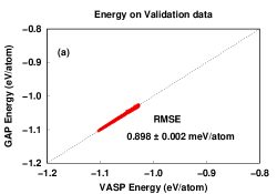
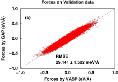
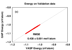
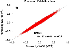
Figure 1: Comparison between DFT and GAP-predicted energy and forces for Model M1. Figure 1(a) and (b) corresponds to M1-1 and Figure 1(c) and (d) corresponds to M1-3.

It may be noted that the standard RMS values are averages. Since, we wish to carry out long MD simulations at temperature slightly above the melting temperatures, the errors in forces can become critical. Therefore, after examining the errors in the forces of individual atom along with errors in the energies, we augmented the training data set by adding the configurations near the points having absolute force above a certain value, leading to an increase of 100-150 data points in the training data set. In the present case, the errors turn out to be uniformily distributed (see Figure 1). Therefore, it was convenient to increase the number of data points uniformily over the entire energy range. The models were retrained, and this process was carried out iteratively until the maximum error in the forces was less than 0.1%. With this procedure, the final size of the training data set was about 1900 configurations. This is designated as model M1.

In Figure 1, we show the comparison between DFT quantities and GAP results of energies and forces for validation data. Figure 1(a) and Figure 1(b) correspond to M1-1 and Figure 1(c) and Figure 1(d) correspond to M1-3. It can be seen that there is dramatic improvement in the accuracy of the model. The RMS values for energy and forces for final model M1-3 are 0.438 meV/atom and 19.197 meV/$\AA$ respectively. As shown in the Table 2, the maximum error in the force is of the order of 0.1$\%$. In fact, we have examined the absolute error in energy and forces for the all the validation configurations. These plots are shown in supplementary information S5 and S6.

Table 2: Maximum percentage errors in energy and forces during training of Na₅₅. Out of several training sessions, three representative ones are shown. The maximum of all forces (3 $\times$ number of configuration $\times$ N) is noted.

Model	Configurations		Maximum percentage Error
	Training	Validation	Training	Validation	Training	Validation
M1-1	544	1899	0.532	0.938	0.509	0.562
M1-2	630	1101	0.033	0.353	0.096	0.108
M1-3	1945	4184	0.024	0.311	0.113	0.129

The model M1 was successfully used in computing the specific heat for Na₅₅. However, when the model was employed to test larger systems up to $N=250$, in some cases the errors in the energies and the percentage error in the forces increased up to about 32 meV and 40 $\%$, respectively. This impelled us to improve on model M1 by including data points from other cluster sizes. Typically, we included 20-50 data points for each cluster of sizes N=40-55, 60, 70, 80, 90, 92, 116, 138, 147, 178, and 200. The resultant model is designated model M2. The comparison between model M1 and M2 is given in Table 3. It is gratifying to see that the absolute errors in the energies reduce significantly to less than 0.94 meV. We also examine the maximum force for all the case and is found to less than 0.11$\%$. (see supplementary information S7 and S8.)

Table 3: Maximum absolute error in energy, Mean absolute error (MAE) and root mean square error (RMSE) for validation sets of various sodium clusters. The unit of energy is given in meV/atom.

System	No. of Configs	Error in Energy (meV/atom)
		Absolute		MAE		RMSE
		M1	M2	M1	M2	M1	M2
70	2541	28.729	4.76	24.563	0.828	24.614	1.062
80	6178	35.098	5.08	30.477	0.833	30.556	1.092
90	1355	49.752	2.79	44.868	0.644	44.960	0.849
92	2045	60.888	2.87	51.500	0.876	51.621	1.127
116	3556	59.536	1.61	56.576	0.391	56.593	0.488
138	4324	90.624	0.94	87.214	0.140	87.223	0.191
147	3672	82.865	1.16	80.778	0.170	80.784	0.229
178	1372	91.929	1.23	89.866	0.236	89.872	0.346
200	2148	99.451	1.53	95.815	0.217	95.821	0.296

For this final model M2, 1213 data points were used of which only 50 data points per cluster were used from the large size clusters. It is of some interest to point out that for the case of large cluster e.g. Na₂₀₀, each data point generates about 200 neighbourhoods or 200 finite-sized clusters which is nearly 4 times larger than those generated by the 55-atom cluster. Thus, adding only a few data points of clusters with a larger number of atoms, improves the quality of the model significantly (see supplementary information S9). Indeed, model M2 (the final best model) required a RAM of more than 650 GB.

3 Results and Discussion

We now employ these models to obtain the thermodynamics properties, specifically heat capacities of Na₅₅ and Na₁₄₇, as well as to obtain the isomers of Na₁₄₇, Na₂₀₀, Na₂₀₁, and Na₂₅₂ clusters. We start with a discussion of the thermodynamic properties.

3.1 Thermodynamics

We have used the well-established and well-tested multiple histogram methods for computing specific heat. For the multiple histogram method density of accessible states $\Omega(V,T)$, are required for a large range of temperatures. Care is taken to ensure that there is sufficient overlap between the adjacent histograms. This essentially decides the choice of temperature intervals. For more details of the multiple histogram method, the reader is referred to the articles [57, 58]. We have carried out molecular dynamics simulations using the LAMMPS package [7] with GAP models M1 and M2. We have computed the heat capacities for Na₅₅ and Na₁₄₇.

The multiple histograms are generated by performing MD simulations at 21 different temperatures ranging from 60 K to 330 K for both clusters, with a time step of  2 fs using Nosé-Hoover thermostat leading to a total simulation time of 400 ps per temperature. All simulations began with the lowest energy structure as obtained by our models. We have used the GAP model M1 for Na₅₅ and model M2 for Na₁₄₇. The lowest energy structures for Na₅₅ and Na₁₄₇ are icosahedra. The ground state structure of Na₁₄₇ is shown in Figure 4. It agrees very well with our earlier density-functional result [51]. Figure 4 also depicts the lowest energy structures of Na₂₀₀, Na₂₀₁ and Na₂₅₂ clusters. The multiple histogram obtained for Na₅₅ and Na₁₄₇ are shown in Figure 2. A clear separation of peaks between two temperatures 270 K and 290 K indicates the temperature range of melting. This feature should also be reflected in a peak in the heat capacity plot.

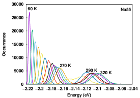
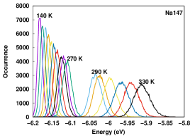
Figure 2: The multiple histograms showing the potential energy distribution for Na₅₅ and Na₁₄₇. At higher temperatures the histograms are much wider, indicating liquid-like behaviour.

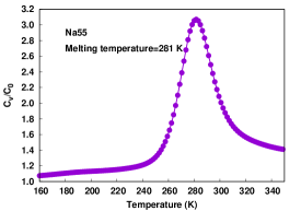
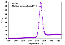
Figure 3: Heat capacity curves for Na₅₅ to Na₁₄₇ using MD simulation with GAP model. The heat capacity curves are scaled C₀, where C₀=(3N-9/2)k_B is the zero temperature classical limit of the rotational plus vibrational canonical specific heat.

The resulting heat capacities $C_{v}/C_{0}$, where C₀=(3N-9/2)k_B is the zero temperature classical limit of the rotational plus vibrational canonical specific heat as a function of temperature $T$ for Na₅₅ (model M1) and Na₁₄₇ (model M2) clusters are shown in Figure 3. It can be observed that the melting temperatures identified by the peaks in the heat capacities are 281 K ($\pm 10$ K) and 271 K ($\pm 10$ K), for Na₅₅ and Na₁₄₇, respectively. There is an excellent agreement between the melting temperatures obtained in this work with those measured experimentally by Haberland et. al. as well as with earlier reported density-functional calculations [50]. Note that the reported experimental values by Haberland et. al. are 290 K and 272 K for Na₅₅ and Na₁₄₇, respectively. This is the first reported result on specific heat calculations of Na₁₄₇ using machine learning potential with density-functional accuracy.

The above discussion clearly shows that the GAP models we developed are accurate enough for sodium clusters. As we shall see, the models can be extended to obtain isomers and even thermodynamics of clusters of sizes for $N=200,201$ and 252 sodium atoms. It may be noted that the time taken by the GAP model to carry out the MD simulation over that of the ab initio methods is tremendously decreased [59]. We have exploited this fact to obtain 40 isomers each for $N=147,200,201$ and 252.

3.2 Isomers using GAP Model M2

We now turn our attention to obtaining isomers of clusters of sizes of more than 150 atoms. Specifically, we present results for 40 isomers of sodium clusters of sizes $N=147,200,201$, and $252$. It may be noted that the previous density-functional studies on sodium clusters are mainly restricted to $\leq$ 150 atoms [51, 52], most of them being below 100 atoms [60].

Table 4: Percentage error in energies and bond length of few lowest energy isomers generated using GAP model M2. $n$ is the isomer number.

	Na147						Na200
	Energy (eV)			Bondlength (Å)			Energy (eV)			Bondlength (Å)
$n$	VASP	GAP	Error	VASP	GAP	Error	$n$	VASP	GAP	Error	VASP	GAP	Error
1	-170.6213	-170.9273	0.1793	3.493	3.494	0.0001	1	-234.8059	-235.1887	0.1630	3.366	3.360	0.165
2	-170.4499	-170.7899	0.1994	3.441	3.265	5.110	2	-234.2854	-234.6999	0.1769	3.336	3.289	1.399
3	-170.3532	-170.6974	0.2020	3.306	3.263	1.324	3	-234.3508	-235.2440	0.3811	3.339	3.315	0.732
4	-170.1236	-170.6238	0.2940	3.263	3.260	0.091	4	-233.2936	-234.4981	0.5163	3.280	3.276	0.137
5	-169.3874	-170.1951	0.4768	3.260	3.267	0.236	5	-233.2315	-234.3009	0.4584	3.292	3.289	0.098
6	-168.7203	-170.0023	0.7598	3.267	3.212	1.693	6	-231.7990	-233.3538	0.6707	3.313	3.284	0.883
7	-168.6236	-169.8945	0.7536	3.230	3.235	0.157	7	-232.4981	-233.6663	0.5024	3.255	3.278	0.722
8	-168.5279	-169.8162	0.7644	3.247	3.230	0.527	8	-232.0359	-233.4958	0.6291	3.279	3.292	0.396
9	-168.3992	-169.4272	0.6104	3.248	3.273	0.785	9	-232.2099	-233.3486	0.4903	3.311	3.294	0.527
10	-167.7377	-169.1585	0.8470	3.285	3.274	0.350	10	-232.3758	-233.4144	0.4469	3.226	3.204	0.665
	Na201						Na252
	Energy (eV)			Bondlength (Å)			Energy (eV)			Bondlength (Å)
$n$	VASP	GAP	Error	VASP	GAP	Error	$n$	VASP	GAP	Error	VASP	GAP	Error
1	-235.2917	-236.8940	0.6810	3.269	3.410	4.308	1	-296.6961	-298.5249	0.6164	3.332	3.363	0.924
2	-235.2835	-236.8564	0.6685	3.316	3.437	3.621	2	-296.6267	-298.5029	0.6324	3.370	3.379	0.264
3	-235.2445	-236.7578	0.6432	3.250	3.390	4.310	3	-296.6022	-298.4893	0.6362	3.413	3.379	0.991
4	-235.1744	-236.6899	0.6444	3.231	3.286	1.698	4	-296.6018	-298.4621	0.6272	3.383	3.270	3.336
5	-235.1206	-236.4845	0.5800	3.261	3.393	4.029	5	-296.5856	-298.4434	0.6263	3.398	3.341	1.677
6	-234.9514	-236.4387	0.6330	3.236	3.289	1.620	6	-296.5463	-298.4230	0.6328	3.402	3.337	1.886
7	-233.5629	-235.5166	0.8364	3.260	3.285	0.752	7	-296.5218	-298.4002	0.6335	3.383	3.342	1.198
8	-233.3826	-235.4676	0.8933	3.185	3.293	3.383	8	-296.4960	-298.3887	0.6383	3.386	3.329	1.702
9	-233.3317	-235.4161	0.8933	3.273	3.293	0.590	9	-296.4904	-298.3555	0.6290	3.364	3.326	1.114
10	-233.3260	-235.3186	0.8539	3.293	3.273	0.586	10	-296.4846	-298.3180	0.6183	3.291	3.292	0.014

First, let’s discuss the method of obtaining the isomeric structures. We have carried out extensive MD simulations of the order of 400 ps for each cluster at six temperatures in the range of 100 K-300 K. This gave a total of 1.2 million configurations, from which we choose every 100^th configurations for local minimization. The configurations were then sorted according to their energies, and only one in the set of all degenerate configurations that lay within $\Delta{E}~{}\leq~{}0.01eV$ were selected. This led to about 200 structures that were used for local minimization using the M2 model. These 200 structures were further scrutinized for any duplicates giving only about 40 distinct structures per cluster.

To assess the accuracy of the GAP model, the 20 lowest energy structures were further optimized using DFT. A comparison between the total energies and bond lengths, giving percentage error for the 10 lowest structures are presented in Table 4. In all the cases the error in energy is less than 0.9%. While the errors in bondlength for Na₁₄₇ and Na₂₀₀ are less than 1% (with four exceptions). The errors are slightly more for Na₂₀₁. The mean absolute error ($|E_{DFT}~{}-~{}E_{GAP}|$) is less than 7 meV/atom, the smallest and largest errors being 1.9 meV/atom and 10.3 meV/atom respectively. Thus, it can be observed that geometries obtained with the GAP models are in good agreement with those computed by DFT. It may be emphasize that only a few iterations by VASP were required to get equilibrium structures.

Figure 4: Ground state structures of Na₁₄₇, Na₂₀₀, Na₁₄₇, and Na₂₅₂ sodium clusters.

Figure 5: Lowest-energy structures of Na₁₄₇, Na₂₀₀, Na₁₄₇, and Na₂₅₂ sodium clusters.

In Figure 4, the lowest energy geometries for Na₁₄₇, Na₂₀₀, Na₂₀₁, and Na₂₅₂ are shown. Some representative geometries of low and high energy isomers are shown in Figure 5. We can see from Figure 4, the lowest-energy structure of Na₁₄₇ is complete icosahedron. The shapes of the 200 and 201 atoms clusters can be understood as distorted icosahedron surrounded by the remaining atoms, forming a partial third shell on one side. This gives these geometries a non-spherical shape. Interestingly, addition of extra atom to Na₂₀₀, changes the shape significantly. In Na₂₀₁, third shell is far more spherical than Na₂₀₀. From Figure 4, we see significant differences in the structural features of the Na₂₀₀ and Na₂₀₁ clusters. The geometries of both clusters are quite distorted. The 252-atom sodium cluster is also distorted, and yet very different from those of 200 and 201-atom clusters. Here, the shape is nearly spherical.

Figure 5 shows some of the high-energy structures of sodium clusters. In each of the cases, the first isomer shown is closest in energy to the gound state. The remaining high energy structures are randomly selected. It is observed that the high-energy structures are considerably distorted. The computing the ground state and equilibrium geometries are non-trivial, especially for for large clusters. A systematic understanding of evolution of geometries, ordering of isomers and nature of high energy isomers is beyond the scope of present work. In this work, we have developed machine learned model which is accurate enough to address some of these problems.

4 Summary and Conclusion

We have developed machine-learned Gaussian Approximation Potential models for constructing the potential energy surfaces for sodium clusters for a wide range of sizes. We demonstrate that about 1300 data points are sufficient to yield very accurate models. These models have been used to compute the thermodynamic properties of Na₅₅ and Na₁₄₇ using multiple histogram method. The results of the model are in excellent agreement with experimental heat capacity curves as well as DFT results. The models has enabled us to compute the heat capacity curve and melting temperature of Na₁₄₇ which has not been previously reported. In addition, up to 20 isomers of the larger cluster ($N\geq 200$) that were difficult to obtain with the accuracy of DFT have been reported with density-functional accuracy. Global optimization of cluster geometry of large sizes is known to be highly compute intensive. Our work demonstrates that ML model paves a way for obtaining several isomers of large clusters of sodium. Even without additional minimization by DFT, used in the present work, the total energy and geometries are fairly accurate. Having established the accuracy of GAP models, it is tempting to employ the models to explore several properties of much larger clusters which were not accessible with limited computational resources. We hope the availability of such models will open up a way to investigate physics of large clusters.

5 Acknowledgements

One of us (DGK) is pleased to acknowledge a number of useful discussions with Dr. Balchandra Pujari, Centre for Modeling and Simulation, SPPU, Pune and Dr Sandip De, BASF, Germany.

6 CRediT authorship contribution statement

All results have been obtained by equal contributions of the authors.

7 Declaration of competing interest

The authors declare that they have no known competing financial interests or personal relationships that could have appeared to influence the work reported in this paper.

8 Data Availability

The data used in training and validation as well as model parameters have been provided in the supplementary information. In addition, the coordinates of isomer geometries obtained with GAP and VASP are also available.

References

- [1] Daan Frenkel and Berend Smit. Understanding Molecular Simulation:From Algorithms to Applications. Elsevier, 2023.
- [2] Smith A., Jones B., and Doe C. Molecular dynamics simulations: A powerful tool for interdisciplinary research. J. Phys. Chem., 124(15):5678–5685, 2000.
- [3] Johnson D. and Brown E. Advancements in molecular dynamics codes: From theory to applications. Progess in Physics, 72(3):123–145, 2005.
- [4] Marco De Vivo, Matteo Masetti, Giovanni Bottegoni, and Andrea Cavalli. Role of molecular dynamics and related methods in drug discovery. J.Med, Chem., 59(9):4035, 2016.
- [5] G. Ciccotti, C. Dellago, M. Ferrario, E. R. Hernández, and M. E. Tuckerman. Molecular simulations: past, present, and future. Eur. Phys. J. B., 95:3:1–22, 2022.
- [6] S Gowthaman. A review on mechanical and material characterisation through molecular dynamics using large-scale atomic/molecular massively parallel simulator (lammps). Functional Composites and Structures, 5(1):012005, 2023.
- [7] S. Plimpton. Fast parallel algorithms for short-range molecular dynamics. J. Mole. Phys., 117:1–19, 1995.
- [8] Abraham M. Murtola, T Schulz R Páll, S Smith, and J. Hess B. Lindah E. Gromacs: High performance molecular simulations through multi-level parallelism from laptops to supercomputers. SoftwareX, 1-2:19–25, 2015.
- [9] J.D. Gale. GULP-a computer program for the symmetry adapted simulation of solids. JCS Faraday Trans., 93:629, 1997.
- [10] Jorge José Kohanoff. Electronic Structure Calculations for Solids and Molecules:Theory and Computational Methods. Cambridge University Press, 2006.
- [11] Richard M. Martin. Electronic Structure Basic Theory and Practical Methods. Cambridge University Press, 2020.
- [12] Car R. and Parrinello M. Unified approach for molecular dynamics and density-functional theory. Phys. Rev. Lett., 55(22):2471–2474, 1985.
- [13] Jórg Behler and Michele Parrinello. Generalized neural-network representation of high-dimensional potential-energy surfaces. Phys. Rev. Lett., 98:146401, 2007.
- [14] J’́org Behler. Neural network potential-energy surfaces in chemistry: a tool for large-scale simulations. Phys. Chem. Chem. Phys., 13:17930–17955, 2011.
- [15] Bartók A. P., Mike C. Payne, Kondor R, and Csányi G. Gaussian approximation potentials: The accuracy of quantum mechanics, without the electrons. Phys. Rev. Lett., 104:136403, 2010. https://github.com/libAtoms/GAP.
- [16] S. Alireza Ghasemi, Albert Hofstetter, Santanu Saha, and Stefan Goedecker. Interatomic potentials for ionic systems with density functional accuracy based on charge densities obtained by a neural network. Phys. Rev. B, 92:045131, 2015.
- [17] Zhang L., Han J., and Car R. Deep potential molecular dynamics: A scalable model with the accuracy of quantum mechanics. Phys. Rev. Lett., 120(14):143001, 2018. https://github.com/deepmodeling/deepmd-kit/tree/master.
- [18] Yunxing Zuo, Chi Chen, Xiangguo Li, Zhi Deng, Yiming Chen, Jórg Behler, Gábor Csányi, Alexander V. Shapeev, Aidan P. Thompson, Mitchell A. Wood, and Shyue Ping Ong. Performance and cost assessment of machine learning interatomic potentials. J. Phys. Chem. A, 124:731–745, 2020.
- [19] Max Pinheiro Jr, Fuchun Ge, Nicolas Ferré, Pavlo O. Dral, and Mario Barbatti. Choosing the right molecular machine learning potential. Chemical Science, 12:14296, 2021.
- [20] Ivan S Novikov, Konstantin Gubaev, Evgeny V Podryabinkin, and Alexander V Shapeev. The MLIP package: moment tensor potentials with mpi and active learning. Mach. Learn.:Sci. Technol., 2(2):025002, 2020.
- [21] A. Rohskopf, C. Sievers, N. Lubbers, N. Lubbers, M. A. Cusentino, J. Goff, J. Janssen, M. McCarthy, D. Montes de Oca Zapain, S. Nikolov, K. Sargsyan, D. Sema, E. Sikorski, L. Williams, A. P. Thompson, and M. A. Wood. FitSNAP: Atomistic machine learning with LAMMPS. Journal of Open Source Software, 8(84):5118, 2023.
- [22] Brown L, Chen X, and Lee J. Machine learning interatomic potentials for materials. Annu. Rev. Mater. Res., 49(1):463, 2019.
- [23] Jörg Behler and Gábor Csányi. Machine learning potentials for extended systems: a perspective. Eur. Phys. J. B., 94:142, 2021. https://www.uni-goettingen.de/de/560580.html.
- [24] Bartók A. P., Kondor R, and Csányi G. On representing chemical environments. Phys. Rev. B, 87(18):184115, 2013.
- [25] Albert P. Bartók and Gabor Csányi. Gaussian approximation potentials: A brief tutorial introduction. International Journal of Quantum Chemistry, 115:1051–1057, 2015.
- [26] Ilyes Batatia, David Peter Kovacs, Gregor N. C. Simm, Christoph Ortner, and Gabor Csanyi. MACE: Higher order equivariant message passing neural networks for fast and accurate force fields. In Alice H. Oh, Alekh Agarwal, Danielle Belgrave, and Kyunghyun Cho, editors, Advances in Neural Information Processing Systems, 2022. https://github.com/ACEsuit/mace.
- [27] Ilyes Batatia, Simon Batzner, Dávid Péter Kovács, Albert Musaelian, Gregor N. C. Simm, Ralf Drautz, Christoph Ortner, Boris Kozinsky, and Gábor Csányi. The design space of E(3)-equivariant atom-centered interatomic potentials, 2022.
- [28] Justin S. Smith, Benjamin Nebgen, Nithin Mathew, Jie Chen, Nicholas Lubbers, Leonid Burakovsky, Sergei Tretiak, Hai Ah Nam, Timothy Germann, Saryu Fensin, and Kipton Barros. Automated discovery of a robust interatomic potential for aluminum. Nature Communications, 12:1257, 2021.
- [29] Chen C. and Ong S. P. A universal graph deep learning interatomic potential for the periodic table. Nat. Comput. Sci., 2:718–728, 2022.
- [30] Y. Mishin. Machine-learning interatomic potentials for materials science. Acta Materialia, 214:116980, 2021.
- [31] Oliver T. Unke, Stefan Chmiela, Huziel E. Sauceda, Michael Gastegger, Igor Poltavsky, Kristof T. Schütt, Alexandre Tkatchenko, and Klaus-Robert Müller. Machine learning force fields. Chemical Reviews, 121:10142, 2021.
- [32] Tongqi Wen, Linfeng Zhang, Han Wang, Weinan, and David J. Srolovitz. Deep potentials for materials science. Materials Futures, 1(2):1–28, 2022.
- [33] Atsuto Seko. Machine learning potentials for multicomponent systems: The Ti-Al binary system. Phys. Rev. B, 102:174104, 2020.
- [34] Geng Sun and Philippe Sautet. Toward fast and reliable potential energy surfaces for metallic Pt clusters by hierarchical delta neural networks. J. Chem. Theory Comput., 15 (10):5614–5627, 2019.
- [35] Siva Chiriki and Satya S. Bulusu. Modeling of dft quality neural network potential for sodium clusters: Application to melting of sodium clusters (na20 to na40). Chem. Phys. Lett., 652:130–135, 2016.
- [36] Yunzhe Wang, Shanping Liu, Peter Lile, Sam Norwood, Alberto Hernandez, Sukriti Manna, and Tim Mueller. Accelerated prediction of atomically precise cluster structures using on-the-fly machine learning. npj Computational Materials, 8(173):1–10, 2022.
- [37] Mozhdeh Shiranirad, Christian J. Burnham, and Niall J. English. Machine-learning-based many-body energy analysis of Argon clusters: Fit for size? Chemical Physics, 552:111347, 2022.
- [38] Marco Fronzi, Roger D. Amos, and Rika Kobayashi. Evaluation of machine learning interatomic potentials for gold nanoparticles-transferability towards bulk. Nanomaterials, 13(12):1832, 2023.
- [39] Gunnar Schmitz and Ove Christiansen. Gaussian process regression to accelerate geometry optimizations relying on numerical differentiation. J. Chem. Phys., 148:241704, 2018.
- [40] G. Deringer, V. L. Csányi. Machine learning based interatomic potential for amorphous carbon. Phys. Rev. B, 95:094203, 2017.
- [41] Behler J. and Parrinello M. Gaussian approximation potentials: A brief overview. Springer, 2019.
- [42] Shapeev A. V. Moment tensor potentials: A class of systematically improvable interatomic potentials. Multiscale Model Simul., 14(3):1153–1173, 2016.
- [43] Kolb B., Lentz L. C., and Shah S. A. Machine learning based molecular dynamics for the mechanical response of metals. J. Mech. Phys. Solids, 137:103856, 2020.
- [44] Artrith N., Urban A., and Ceder G. Efficient and accurate machine-learning interpolation of atomic energies in compositions with many species. Phys. Rev. B, 95(1):014112, 2016.
- [45] Experimentally driven automated machine-learned interatomic potential for a refractory oxide.
- [46] Davis Unruh, Reza Vatan Meidanshahi, Stephen M. Goodnick, Gábor Csányi, , and Gergely T. Zimányi. Gaussian approximation potential for amorphous Si : H. Phys. Rev. Materials, 6:065603, 2022.
- [47] Martin Schmidt, Robert Kusche, Bernd von Issendorff, and Hellmut Haberland. Irregular variations in the melting point of size-selected atomic clusters. Nature, 393:238.
- [48] Martin Schmidt and Hellmut Haberland. Phase transitions in clusters. C. R. Physique, 3:327–340, 2002.
- [49] M. Schmidt and H. Haberland. C. R. Physique, 3:327–340, 2002.
- [50] S. Chacko, D. G. Kanhere, and S. A. Blundell. First principles calculations of melting temperatures for free na clusters. Phys. Rev. B, 71:155407, 2005.
- [51] Seyed Mohammad Ghazi, Shahab Zorriasatein, , and D. G. Kanhere. Building clusters atom-by-atom: From local order to global order. J. Phys. Chem. A, 113:2659–2662, 2009.
- [52] Melting in large sodium clusters: An orbital-free molecular dynamics study.
- [53] Qunchao Tong, Pengyue Gao, Hanyu Liu, Yu Xie, Jian Lv, Yanchao Wang, and Jijun Zhao. Combining machine learning potential and structure prediction for accelerated materials design and discovery. J. Phys. Chem. Lett., 11(20):8710–8720, 2020.
- [54] G. Kresse and J. Hafner. Ab initio molecular dynamics for liquid metals. Phys. Rev. B, 47:558, 1993. http://cms.mpi.univie.ac/at/vasp.
- [55] G. Kresse and D. Joubert. From ultrasoft pseudopotentials to the projector augmented-wave method. Phys. Rev. B, 59:1758, 1999.
- [56] J. P. Perdew, K. Burke, and M. Emzerhof. Generalized gradient approximation made simple. Phys. Rev. Lett., 77:3865, 1996.
- [57] A. M. Ferrenberg and R. H. Swendsen. New Monte Carlo technique for studying phase transitions. Phys. Rev. Lett., 61:2635, 1988.
- [58] Prachi Chandrachud, Kavita Joshi, and D. G. Kanhere. Thermodynamics of carbon-doped al and ga clusters: Ab initio molecular dynamics simulations. Phys. Rev. B, 76:235423, 2007.
- [59] In a test simulation for 10,000 MD steps with a timestep of 3 fs we got a scaling of about 300 times by LAMMPS over VASP.
- [60] Sukriti Manna, YunzheWang, Alberto Hernandez, Peter Lile, Shanping Liu1, and Tim Mueller. A database of low-energy atomically precise nanoclusters. Scientific Data, 10:308, 2023.