A Novel Neural-symbolic System under Statistical Relational Learning

Abstract

A key objective in field of artificial intelligence is to develop cognitive models that can exhibit human-like intellectual capabilities. One promising approach to achieving this is through neural-symbolic systems, which combine the strengths of deep learning and symbolic reasoning. However, current approaches in this area have been limited in their combining way, generalization and interpretability. To address these limitations, we propose a general bi-level probabilistic graphical reasoning framework called GBPGR. This framework leverages statistical relational learning to effectively integrate deep learning models and symbolic reasoning in a mutually beneficial manner. In GBPGR, the results of symbolic reasoning are utilized to refine and correct the predictions made by the deep learning models. At the same time, the deep learning models assist in enhancing the efficiency of the symbolic reasoning process. Through extensive experiments, we demonstrate that our approach achieves high performance and exhibits effective generalization in both transductive and inductive tasks.

Human cognitive systems consist of perception and reasoning. Specifically, perception is primarily responsible for recognizing information, while reasoning is responsible for thinking and logically deducing information. When humans process information, they combine both perception and reasoning to maximize their ability to comprehend and analyze information. Artificial intelligence (AI) systems already exist that possess either perception or reasoning capabilities. For instance, deep learning models excel at perception and have achieved remarkable performance in various perception tasks. They demonstrate inductive learning capabilities and computational efficiency. In contrast, symbolic logic is adept at logical reasoning and has yielded impressive results in reasoning tasks. It boasts deductive reasoning abilities, generalization, and interpretability. However, both types of models still have their limitations. Deep learning models often operate as black boxes, lacking interpretability, exhibiting weak generalization, and requiring large amounts of training data to perform satisfactorily. Conversely, symbolic logic relies on search algorithms to find solutions in the search space, which can result in slow reasoning when confronted with large search spaces. Hence, by combining and leveraging the strengths of both approaches, we can integrate the processes of perception and reasoning into a unified framework, mimicking the human cognitive system more effectively. Indeed, Leslie G. Valiant, the Turing Award winner, considers that reconciling the statistical nature of learning and the logical nature of reasoning to build a cognitive computing model that integrates concept learning and concept manipulation is one of the three fundamental problems and challenges of computer science valiant2003three .

The neural-symbolic system is a promising approach that successfully integrates perception and reasoning into a unified framework belle2020symbolic ; Hitzler2021NeuroSymbolicAI ; curry2022multimodal . Various neural-symbolic systems have emerged, which can be broadly classified into three categories yu2021recent : learning for reasoning methods, reasoning for learning methods, and learning-reasoning methods. Learning for reasoning methods qu2019probabilistic ; zhang2020efficient ; mao2019neuro primarily focus on symbolic reasoning. Reasoning for learning approaches xu2018semantic ; xie2019embedding ; luo2020context primarily emphasize the role of deep learning models. Only a few studies explore learning-reasoning methods to achieve a more comprehensive integration manhaeve2021neural ; zhou2019abductive . While these approaches has made significant progress in neural-symbolic systems field, it remains an open problem that requires further exploration and research.

This paper introduces a novel framework, called the general bi-level probabilistic graph reasoning framework (GBPGR), to integrate deep learning models with symbolic reasoning in a mutually beneficial manner. In GBPGR, symbolic reasoning assists the deep learning models by making their predictions more logical, consistent with common sense, and interpretable, thereby improving their generalization capabilities. On the other hand, the deep learning models aid symbolic reasoning by enhancing their efficiency and robustness to noise. Symbolic reasoning takes inputs from deep learning and learns a joint probability distribution based on first-order logic (FOL). This joint probability distribution is then used to infer the values of arbitrary variables. However, there are two challenges when building the two-layer structure: (1) how to combine both deep learning and symbolic reasoning to model a joint probability distribution with FOL; (2) how to train it in an end-to-end pose. Overcoming these challenges is crucial for successfully implementing the GBPGR framework.

The proposed GBPGR framework leverages the techniques of statistical relational learning (SRL) to address the challenge (1). SRL combines First-order logics (FOLs, relation models) and probabilistic graphical models (statistical models), serving as a bridge between relational and statistical learning getoor2007introduction . This integration provides logical semantics to probabilistic graphical models and effectively captures uncertainty. Specifically, FOLs are represented as undirected graphs using Markov Logic Networks (MLNs) richardson2006markov as the low-level layer of the GBPGR framework. MLNs enable the unification of FOLs and probabilistic graphical models into a single representation domingos2019unifying . The prediction results of the deep learning models serve as nodes in the high-level layer. To establish connections between the two layers of the framework, edges are created based on identifiers and the number of variables in the predicate. This process enables constructing a joint probability distribution involving both the probabilistic graphical model with FOLs and the deep learning models. By incorporating SRL techniques and building a joint probability distribution, the GBPGR enables the integration of symbolic reasoning and deep learning models, thereby facilitating a mutually beneficial interaction between perception and reasoning processes.

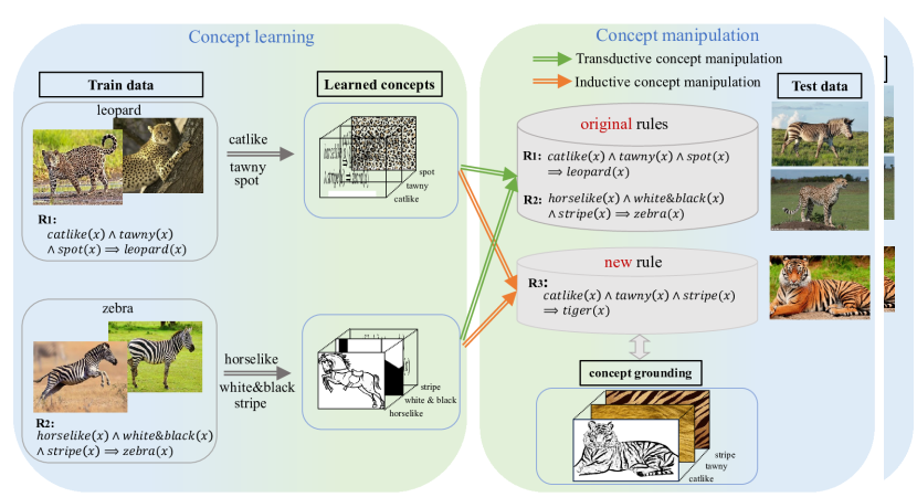
Figure 1: Overview of GBPGR. The concept learning aims to acquire fundamental concepts such as “catlike”, “tawny” and “spot” from train data. In transductive concept manipulation, the learned concepts and the original rules are employed to test data whose labels have occurred in the training sets. Incorporating these learned concepts endows GBPGR with interpretability, as it provides insights into how the prediction results are derived based on them in conjunction with the rules. Conversely, in inductive concept manipulation, the function of the learned concepts as the rule body, and new rules are introduced to reason the result when testing a new sample whose label has never appeared in the training set.

To address the challenge (2), we use the variational EM algorithm to train the model. Specifically, the workflow of GBPGR contains two steps: concept learning and concept manipulation, as shown in Fig. 1. During concept learning, the deep learning models learn a mapping function from the training data to concepts, such as “stripe”. Subsequently, these acquired concepts serve as elements for symbolic reasoning, allowing the model to learn a joint probability distribution and infer results. Once the model is trained, it can execute concept manipulations in both transductive and inductive scenarios. In the transductive settings, the model recognizes samples within the training data. In the inductive scenario, the model recognizes samples not encountered during the training process through symbolic reasoning. This capacity for symbolic reasoning enables the model to handle previously unseen data and extend its capabilities beyond the training set.

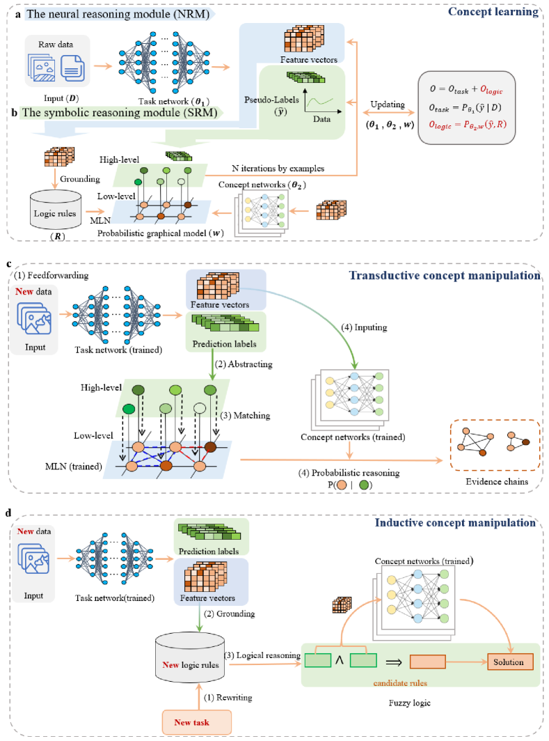
Figure 2: Illustration of concept learning and manipulation. a, NRM aims to predict labels for raw data and output pseudo-labels and feature vectors. b, SRM is a bi-level probabilistic graphical model, where the high-level layer represents the prediction results (pseudo-labels) generated by NRM. In contrast, the low-level layer consists of the ground atoms of logic rules, which are grounded by feature vectors and concept networks. The whole model is trained end-to-end, using backpropagation to revise pseudo-labels. c, Transductive manipulation. d, Inductive manipulation.

In our previous conference paper yu2022probabilistic , we provided an initial presentation and validation of the proposed idea on visual relationship detection. However, this current study significantly extends that work by including new tasks such as digit image addition and zero-shot image classification, new baseline models and extensive experimental validations and comparisons.

Results

Overview of GBPGR

An overview of GBPGR, consisting of two important phases (i.e., concept learning and concept manipulation), is shown in Fig. 1.

Concept learning focuses on acquiring fundamental concepts (e.g.,predicates in rules) from train data. For instance, we can learn fundamental concepts like “catlike”, “tawny” and “spot” from images containing leopards, and “horselike”, “white&black” and “stripe” from an image containing zebras, utilizing the rules R1 $\textsf{likecat}(x)\land\textsf{tawny}(x)\land\textsf{spot}(x)\Rightarrow\textsf{leopard}(x)$ and R2 $\textsf{horselike}(x)\wedge\textsf{white\& black}(x)\wedge\textsf{stripe}(x)\Rightarrow\textsf{zebra}(x)$, respectively. In this paper, we use FOLs such as rule body $\Rightarrow$ rule head as our rules.

Concept manipulation aims to infer results that can implement two manipulations such as transductive concept manipulation and inductive concept manipulation. In transductive concept manipulation, the learned concepts and the original rules are employed to test data whose labels have occurred in the training sets. Incorporating these learned concepts endows GBPGR with interpretability, as it provides insights into how the prediction results are derived based on them in conjunction with the rules. For example, the predicted label “leopard” can be attributed to the rule R1. Conversely, in inductive concept manipulation, the learned concepts and the new rules are employed to test data whose label has never appeared in the training set. More concretely, the learned concepts are regarded as the rule body of new rule to reason rule head as the result when testing a new sample. For instance, when an image containing a tiger is fed into the well-trained model, it can trigger the new rule R3 and obtain corresponding concept groundings such as “catlike”, “tawny” and “stripe”. By leveraging R3 and the concept groundings, the model performs reasoning to infer the new concept “tiger”. This approach enables the application of previously learned concepts to new tasks, facilitating reasoning and prediction in a more generalizable manner. Through this process, the model effectively learns, reasons, and generates interpretable results based on the acquired concepts, showcasing its ability to adapt to diverse problem domains and provide valuable insights into the reasoning behind its predictions.

Concept learning

Fig. 2a and Fig. 2b show concept learning. Concept learning includes a neural reasoning module (NRM) and a symbolic reasoning module (SRM). More specifically, NRM is a task network and aims to output pseudo-labels and feature vectors. SRM is a bi-level probabilistic graphical model that is accountable for reasoning results. In SRM, the high-level layer represents the prediction results (pseudo-labels) generated by NRM. In contrast, the low-level layer consists of the ground atoms of logic rules, which are grounded by feature vectors and concept networks. The whole model is trained end-to-end, using backpropagation to revise pseudo-labels. The revised labels from SRM are then adopted to replace pseudo-labels of NRM in the subsequent iteration. After $N$ iterations, the model outputs predicted results of NRM based on symbolic knowledge.

Concept manipulation

As mentioned above, two concept manipulations exist in GBPGR. Thus, we designed two corresponding methods. The first method is transductive, wherein a trained task network is utilized to predict results, and a probabilistic graphical model is employed to provide interpretation, as shown in Fig. 2c. In contrast, the second method is inductive. In this approach, fuzzy logic reasoning is employed to generate output results, accompanied by a reasoning path as the interpretation, as shown in Fig. 2d.

In Fig. 2c, it is worth noting that the training and test sets have overlapping classes such as “zebra”. Our learning process involves training on the training dataset and subsequently making predictions on the test set. More specifically, the steps of transductive manipulation are: (1) inputting new data and obtaining prediction labels through the trained task network; (2) identifying the nodes in the high-level layer based on the prediction labels; (3) matching the nodes in the high-level layer with the logical rules in the MLN to identify the candidate rules; (4) inputting feature vectors to the concept network, retrieving the scores of the concepts, and then applying probabilistic reasoning (Eq. (1)) and fuzzy logic reasoning to obtain the probability score of each rule is true. The rules with high scores are selected as the evidence chain, which interprets the prediction labels. In this paper, we match the prediction results with the low-level nodes to achieve interpretability. If a successful match is achieved, it indicates that the logic rules containing those nodes are triggered, and the corresponding clique composed of those nodes is selected. To quantify the likelihood that the candidate rule is true, we calculate the probability using t-norm fuzzy logic novak2012mathematical . This process enables us to obtain evidence in the form of logic rules that support the reasoning outcomes. To enhance interpretability, we select the most prominent piece of evidence based on the posterior probability $P(R\mid\hat{y})$ as follows.

$$P(R\mid\hat{y})=\prod_{A_{i}\in T_{r}}p({A_{i}}\mid\hat{y}),$$ (1)

where $T_{r}$ is the candidate logic rule here. $A_{i}$ represents grounding atom sets in $T_{r}$ and is a variable in the low-level layer. $\hat{y}$ represents pseudo-labels.

In Fig. 2d, it is important to note that there is no intersection between the training and test data. Specifically, there are three steps for inductive manipulation: (1) rewriting logic rules based on a new task to accommodate specific requirements; (2) grounding the logic rules using feature vectors from task network; (3) inputting the feature vector of the concept mentioned in the rule body of the candidate rules into the concept networks to obtain the labels of the concepts. Then, reason the solution for the new task based on both the rule head and the rule body together. This process can be seen as reprogramming for the new problem, utilizing the learned predicate concepts from the previous step to tackle more complex problem scenarios. For example, the model is trained on single-digit tasks and tested on multi-digit tasks. By adopting this approach, the model can adapt its knowledge and reasoning capabilities to address new problems, thereby showcasing the generalization capabilities of our approach.

Table 1: Test performance of visual relationship detection. The recall results for the top 50/100 in “ReD” and “PhD” are reported, respectively. The best result is highlighted in bold. “$-$” denotes the corresponding result is not provided.

Methods	ReD		PhD		ReD				PhD
	$free\ k$				$k=1$		$k=70$		$k=1$		$k=70$
Recall$@$	50	100	50	100	50	100	50	100	50	100	50	100
Lk distilationyu2017visual	22.7	31.9	26.5	29.8	19.2	21.3	22.7	31.9	23.1	24.0	26.3	29.4
Zoom-Netyin2018zoom	21.4	27.3	29.1	37.3	18.9	21.4	21.4	27.3	28.8	28.1	29.1	37.3
CAI+SCA-Myin2018zoom	22.3	28.5	29.6	38.4	19.5	22.4	22.3	28.5	25.2	28.9	29.6	38.4
MF-URLNzhan2019exploring	23.9	26.8	31.5	36.1	23.9	26.8	$-$	$-$	23.9	26.8	$-$	$-$
zhang2019large	27.0	32.6	32.9	39.6	23.7	26.7	27.0	32.6	28.9	32.9	32.9	39.6
GPS-Netlin2020gps	27.8	31.7	33.8	39.2	$-$	$-$	27.8	31.7	$-$	$-$	33.8	39.2
UVTransEhung2020contextual	27.4	34.6	31.8	40.4	25.7	29.7	27.3	34.1	30.0	36.2	31.5	39.8
NMPhu2022neural	21.5	27.5	$-$	$-$	20.2	24.0	21.5	27.5	$-$	$-$	$-$	$-$
GBPGR	29.4	35.3	36.2	43.0	26.2	29.4	29.4	35.3	32.3	36.4	36.2	43.0

Performance of the GBPGR

To validate the effectiveness of our GBPGR model on performance, generalization and interpretability, we conducted experiments on some challenge tasks, including visual relationship detection (supervised task, transductive concept manipulation) and digit image addition (weakly supervised task, transductive concept manipulation and inductive concept manipulation). In this section, the experimental setup includes datasets, metrics and implementation details, please refer to the section Methods for more information.

Visual relationship detection. In this task, the NRM component of our model follows the architecture described in zhang2019large , and it was trained on the VRD datasets. The experimental results of GBPGR and several state-of-the-art methods are presented in Table 1. We adopt evaluation metrics the same as zhang2019large , including Relationship detection (ReD) and Phrase detection (PhD). Note, $k$ represents candidate relations for each relationship proposal (or $k$ relationship predictions for each object box pair). Since not all state-of-the-art methods specified $k$ in their experiment, we use “$free\ k$” zhang2019large to report results when takes $k$ as a hyper-parameter.

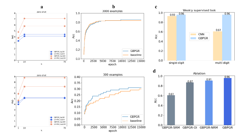
Figure 3: Performance, generalization and ablation results. a, Performance comparisons on digit image addition task (single-addition and multi-addition tasks). b, Performance comparisons with state-of-the-art models (SABR paul2019semantically , MLSE ding2019marginalized , AREN xie2019attentive , LFGAA liu2019attribute , DAZLE huynh2020fine , APN xu2020attribute , CF-ZSL Yang2021collaborative , DUET chen2023duet , MSDN chen2022msdn ) on image classification task (zero-shot learning). The horizontal coordinates indicate different models. c, Generalization comparisons on the visual relationship detection (VRD dataset). Zero-shot learning results of GBPGR and baselines LS-VRU. Larger ReD indicates better results. d, Generalization comparisons on digit image addition task. Quantitative results comparing the generalization performance of GBPGR with the baseline CNN on the test set, using random sampling 300 training samples to train the model. e, Ablation results on digit image addition task. Here is the performance of GBPGR with different loss components. f, Ablation results on the image classification task.

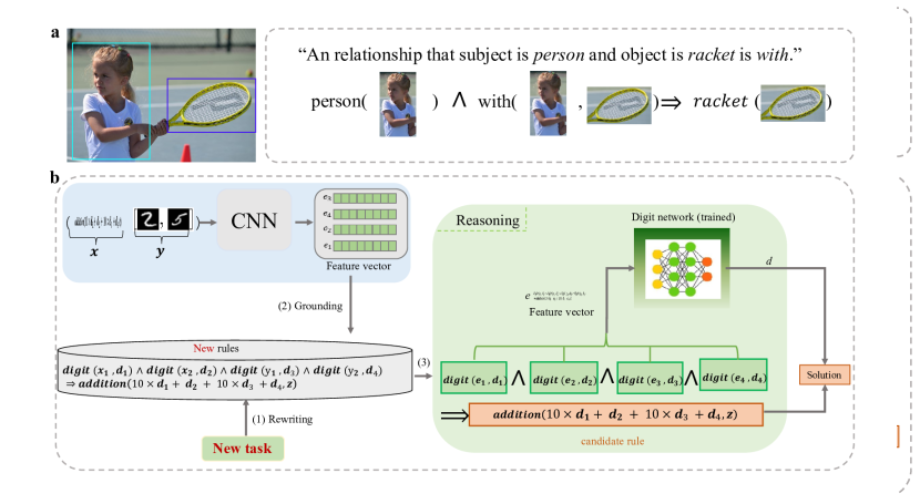
Figure 4: Interpretability analysis. a, An example that can show the interpretability of GBPGR. For example, why is a relationship “next to” between “laptop” and “keyboard” or “mouse” in an image? According to Eq. (1), the model can find the most confident logic rule is $\textsf{laptop}(x)\wedge\textsf{next to}(x,y)\Rightarrow\textsf{keyboard}(y)\vee\textsf{mouse}(y)$. This indicates that the reasoning results of GBPGR are consistent with commonsense. b, Reasoning process of the multi-digit addition. (1) Rewrite logic rules based on multi-digit addition (new task); (2) Grounding rules using feature vectors of $x$ and $y$ from CNN; (3) The process involves inputting the feature vectors associated with the concept mentioned in the candidate rule body into the concept network to obtain the corresponding concept labels. Ultimately, the solution for the new task is achieved by combining the information from both the rule head and rule body, allowing for reasoning and deduction. Note, the variables $x$ and $y$ represent the multi-digit numbers. The symbol $e_{i}$ denotes the feature vector associated with each digit image. Additionally, the variable $d_{i}$ represents the label for each individual digit image, while $z$ represents the label for the addition operation.

In Table 1, the results demonstrate that our GBPGR outperforms state-of-the-art methods in most cases. This can be attributed to the fact that GBPGR can leverage additional information from logic rules, such as the correlation between objects, to learn a more powerful model. Compared to the baseline method LS-VRU zhang2019large , GBPGR achieves significantly better performance. This suggests that the SRM component of GBPGR effectively acts as an error corrector, contributing to improved results.

GBPGR has achieved superior results compared to the baseline methods. The improvement provided by the SRM can be attributed to two key factors. First, the SRM is designed as a probabilistic graphical model that captures dependencies between variables, allowing for more accurate modeling of complex relationships. Second, our logic rules are constructed based on the co-occurrence relationships between predicates, indicating that when one object appears, another object is likely to appear as well. By maximizing the joint probability of the probabilistic graphical model, we effectively maximize the co-occurrence probability during the training phase.

Digit image addition. To evaluate the performance of GBPGR on weakly supervised tasks, we conducted experiments on single-digit addition and multi-digit addition. In this experiment, we input two digit images to GBPGR, and its output is the predicted addition result. The accuracy (Acc) of GBPGR and the CNN baseline on the test set are shown in Fig. 3a. Comparing the results of GBPGR with the CNN baseline, we can observe that GBPGR achieves decent performance. This demonstrates the feasibility of GBPGR in bypassing the need for strong supervised information typically required in pure deep learning approaches. By integrating symbolic knowledge, GBPGR is able to leverage additional supervision signals, such as data labels or relations between data, which leads to improved model performance.

Generalizaton of the GBPGR

We conducted experiments to assess the generalization capabilities of GBPGR. In this study, generalization has two meanings. First, it refers to how well GBPGR performs when it is tested on a new task. For example, the labels of the testing samples are rarely even not contained in the training sets. We validate this generalization in visual relationship detection, image classification and digit image addition. Second, it demonstrates how GBPGR performs once tested on challenging tasks after being trained on easy ones. To verify the second generalizability, we implement experiment on digit image addition task.

Visual relationship detection. we examined the performance of our GBPGR model compared to the baseline LS-VRU in a zero-shot environment. In this scenario, the training and testing data consisted of disjoint sets of relationships from the VRD dataset, as depicted in Fig. 3c. The results indicate that our GBPGR outperforms LS-VRU across different recalls. This highlights the limitations of LS-VRU in handling sparse relationships. In contrast, GBPGR effectively incorporates symbolic knowledge from logic rules and language priors, enabling it to be less affected by sparse relationships and achieve better performance.

Image classification. To evaluate the performance of GBPGR on zero-shot learning, we conducted an experiment on image classification. Fig. 3b presents the results. From the results, we can observe that our GBPGR achieves the best accuracy. This shows that GBPGR can capture common attributes and relationships from seen categories for recognizing unseen categories. In addition, this experiment also illustrates symbolic reasoning with logic rules making the model more robust.

Digit image addition. We proceeded to assess the generalization capability of GBPGR in weakly supervised tasks by comparing it to the baseline CNN. In this context, we validate the generalization performance under various scenarios, including limited training data and learning in a simple task while testing in a more complex task.

In a limited training data scenario, we measured the performance using Acc on the test set with random sampling 300 training samples. As depicted in Fig. 3d, GBPGR consistently achieved higher Acc compared to the CNN. This is because the baseline CNN solely relies on digit image features as input and struggles to train a sufficiently robust model. In contrast, GBPGR leverages both digit image features and the relationships between digit images, such as the relationships encoded in logic rules, enabling it to learn a more effective model.

To validate the learned model in sigle-digit addition can generalize complex task, we introduce multi-digit addition task. In multi-digit addition, the input comprises two lists of images, where each element represents a digit. Each list represents a multi-digit number. The label corresponds to the sum of the two numbers. We visualize this reasoning process in Fig. 4b. In Fig. 3a multi-digit, the result has successfully demonstrated the enhanced prediction accuracy of our multi-digit addition task by leveraging the predicate concepts acquired during the single-digit addition task. Our results show a significant improvement compared to the baseline method. This highlights the flexibility of our model, which is capable of generalizing from simple tasks to more complex ones by modifying the logic rules. Notably, this generalization is achieved due to the shared learnable basic concepts (predicates) between the two tasks.

Interpretibility of the GBPGR

To assess the interpretability of our proposed model, we devised a quantitative method (Eq. (1)) to identify evidence (i.e., the rules) supporting the prediction results. In the case of the supervised and weakly supervised tasks, we visualized the detection results and the interpretability process in Fig. 4a and Fig. 4b, respectively. For instance, the logic rule $\textsf{laptop}(x)\wedge\textsf{next to}(x,y)\Rightarrow\textsf{keyboard}(y)\vee\textsf{mouse}(y)$ makes Eq. (1) get high value, thus this rule is confident for the relationship “next to” in the VRD task Fig. 4a. Fig. 4b shows how GBPGR works with the new rules when dealing with challenging tasks after training on the simple tasks. The simple task involves single-digit addition, represented as $\textsf{digit}(x,d_{1})\wedge\textsf{digit}(y,d_{2})\Rightarrow\textsf{addition}(d_{1}+d_{2},z)$. On the other hand, the challenging task refers to multi-digit addition, represented as $\textsf{digit}(x_{1},d_{1})\wedge\textsf{digit}(x_{2},d_{2})\wedge\textsf{digit}(y_{1},d_{3})\wedge\textsf{digit}(y_{2},d_{4})\Rightarrow\textsf{addition}(10\times d_{1}+d_{2}+10\times d_{3}+d_{4},z)$. By learning the basic concept of “digit” in single-digit addition, we can then generalize this knowledge to the multi-digit addition task through rule reasoning. Based on these figures, we can conclude that our model possesses the capability of self-reasoning, offering commonsense and easily understandable evidence to support its prediction results.

Ablation studies on GBPGR

To investigate how the model trade-off affects reasoning performance, we design three variants to verify the effect of individual components on GBPGR. Specifically, we obtain different variants for optimized objection Eq. (10) (Please refer to Methods) by setting values of the trade-off factors. The three variants are as follows: (1) GBPGR-SRM ($\alpha=1,\beta=0,\gamma=0$): removing symbolic reasoning module. (2) GBPGR-NRM ($\alpha=1/2,\beta=1,\gamma=1$): removing a half of visual reasoning module. (3) GBPGR-OI ($\alpha=1,\beta=1,\gamma=0$): removing crossentropy of observed variables.

We conducted experiments on the MNIST and AwA2 datasets to evaluate the performance of GBPGR and its variants. The results are presented in Fig. 3e and Fig. 3f, respectively. For Fig. 3e, we observe that the performance of the GBPGR-NRM variant is higher compared to its GBPGR-SRM counterparts, which differs from the results on the VRD dataset. This can be attributed to the fact that weakly supervised tasks, such as the MNIST dataset, have limited supervised information. In the case of weakly supervised tasks, the input images do not have their own individual labels, but only the labels for addition. This might result in the NRM module playing a more limited role in the task. Moreover, this finding indicates that leveraging symbolic knowledge is even more important for weakly supervised tasks compared to supervised tasks.

From Fig. 3f, we observe that the correlations among the components of SRM, VRM, and OI have a significantly positive impact on image classification in zero-shot learning. Additionally, we notice that the performance of our model is notably improved when the SRM module is applied. This validates the effectiveness of the logic rules incorporated in our model, as it aligns with our theoretical analysis suggesting that symbolic knowledge in logic rules can rectify the results of the NRM.

Conclusion

In this study, we introduce GBPGR as a general model based on neural-symbolic systems. Our objective is to enhance the performance and generalization of the model, as well as provide interpretability of the results. Additionally, we propose a novel evaluation metric to measure the interpretability of the deep model. Based on our experimental results, we demonstrate that GBPGR surpasses state-of-the-art methods in various reasoning tasks, including supervised and weakly supervised scenarios and zero-shot learning in terms of performance and generalization. Moreover, we emphasize the interpretability aspect of GBPGR by providing visualizations that enhance the understanding of the reasoning process.

Methods

Model definition

We define our model as a function $F$ that takes the raw input $D$ and the pre-defined limited set of logic rules $R$ and maps them to the output $y$ (i.e., $y=F(D,R)$). More specifically, $y=F(D,R)$ can be further simplified as computing a posterior probability $P(y|D,R)$ when provided with input data $D$ and logic rules $R$. Therefore, the learning process of the model can be formulated as a posterior computation problem, which can be defined as follows:

$$\small\forall(D,y)\max P(y|D,R).$$ (2)

In object detection tasks, the input data $D$ represents images, and the output $y$ represents the corresponding labels of objects present in those images. For instance, $D$ could consist of a set of images, and $y$ would contain the object labels such as “cat”,“dog”, etc., indicating the objects recognized in each image. In single-digit addition tasks, the input data $D$ includes pairs of digit images and their corresponding addition operations, while the output $y$ represents the labels for the addition results. For example, $D$ could consist of digit images of “2” and “3”, and $y$ would contain the label “5” as the addition result.

Statistic relation learning

Many tasks in real-world application domains are characterized by the presence of both uncertainty and complex relational structure. Statistical learning focuses on the former, and relational learning on the latter. Statistical relational learning (SRL) seeks to combine the power of both getoor2007introduction .

In this study, we leverage SRL to integrate first-order logic (FOL) and probabilistic graphical models, creating a unified framework that enables probabilistic inference for reasoning problems. To achieve this integration, we employ Markov logic network (MLN) domingos2019unifying , which is a well-known SRL model, to represent logic rules as undirected graphs representing joint probability distributions. In the constructed undirected graph, nodes are generated based on all ground atoms, which are logical predicates with their arguments replaced by specific constants. An edge is established between two nodes if the corresponding ground atoms co-occur in at least one ground FOL. Consequently, a ground MLN can be formulated as a joint probability distribution, capturing the dependencies and correlations among the ground atoms. Thus, a ground MLN can be defined as a joint probability distribution:

$$\small P(A)=\frac{1}{Z(w)}\exp\{\sum_{r\in R}w_{r}\sum_{A_{r}}\phi(A_{r})\},$$ (3)

where $Z(w)$ is the partition function summing overall ground atoms. $A$ is all ground atoms in the knowledge base. $R$ is the set of logic rules and $r$ is a logic rule. $A_{r}$ is ground atom sets in $r$. $\phi$ is a potential function in terms of the number of times the logic rule is true. $w$ is the weight sets of all logic rules. $w_{r}$ represents the weight of a logic rule $r$. The greater weight, the greater confidence of logic rules.

To fully leverage the benefits of deep learning and symbolic reasoning, the GBPGR model needs to fulfill two essential requirements. Firstly, it should be capable of fitting labeled data and enabling joint training, allowing it to learn from both data and symbolic knowledge. Secondly, the model’s predictions should align with symbolic knowledge, indicating that the model’s output should activate relevant logic rules. To address these requirements, we utilize statistical relational learning (SRL) as an interface to connect deep learning and symbolic reasoning in a mutually beneficial manner.

GBPGR includes a neural reasoning module (NRM, it is Fig 2a) and a symbolic reasoning module (SRM, it is Fig 2b). During training, information is propagated from the task network to the SRM fitting labeled data and symbolic knowledge. Therefore, the overall learning objective of the GBPGR is defined as $O$ in Eq. (4).

$$\small O=O_{task}+O_{logic},$$ (4)

where ${O}_{task}$ represents the learning objective of a specific task (objective of the task network), characterizing how well the model’s predictions fit the data. ${O}_{logic}$ is a symbolic reasoning objective (regularization loss), characterizing how well the model’s predictions fit the symbolic knowledge.

Neural reasoning module

A neural reasoning module (NRM, Fig. 2a) is implemented as a deep neural network, where the specific architecture depends on the task at hand, such as visual relationship detection in this paper. The NRM is responsible for predicting labels and outputs feature vectors. The architecture of the NRM may vary depending on the specific task requirements. Considering the previous analysis and Eq. (4) in the paper, the learning objective function of the NRM can be formulated as follows:

$$\small O_{task}=P_{\theta_{1}}(y|D),$$ (5)

where $\theta_{1}$ is the learnable parameter of the NRM.

Symbolic reasoning module

To connect deep learning models with symbolic logic, we utilize SRL to build a probabilistic graphical model in the symbolic reasoning module (SRM). This module consists of a double-layer probabilistic graph, as shown in Fig. 2b, with two types of nodes: the reasoning results of the NRM in the high-level layer and the ground atoms of logic rules grounded by feature vectors in the low-level layer. The high-level layer represents the prediction results of the NRM, while the low-level layer represents MLN. In the low-level layer, MLN is used to connect observed predicates (labeled or appearing in the training data) and unobserved predicates (unlabeled), representing them as a joint probability distribution to infer the probability of unobserved predicates. Between the two layers, we align the prediction results of deep learning models with the ground atoms in logic rules to revise errors. This demonstrates that GBPGR fits both labeled data and symbolic knowledge. Furthermore, MLN plays a crucial role in fitting symbolic knowledge by utilizing joint probabilistic distribution values to quantify the degree of fit for logic rules. The objective of SRM is to use SRLs to learn variables and guide the reasoning of the NRM in the right direction, acting as an error corrector. Our SRM is task-agnostic, and once the probabilistic graphical model is constructed, it can be performed accordingly in the variational expectation-maximization (EM) framework.

Logic rules are a type of commonsense knowledge that is easily understood by humans. In this paper, we consider the FOL language as a means to describe knowledge in the form of logic rules, which offers a strong expressive ability enderton2001mathematical . FOL allows for the definition of any predicates and the description of any relations. In Fig. 2b, the SRM consists of two types of nodes (random variables) and cliques (potential functions). Let $y$ represent the set of high-level nodes, and let $A$ represent the set of low-level nodes, which consist of the ground atoms in the logic rules. A clique $\{\hat{y_{i}},A_{j}\}$ expresses the correlation between the levels. Additionally, subset $A_{r}=\{A_{1},\cdots,A_{m}\}$ represents a clique composed of the ground atoms corresponding to a logic rule $r$, achieved by assigning constants to its arguments. In this study, to obtain the low-level nodes, we need to perform grounding of the logic rules, meaning that predicates are instantiated by constants (which are feature vectors in this paper). To accomplish this, we employ fuzzy logic techniques such as t-norm novak2012mathematical for instantiation. However, if we were to perform grounding for all logic rules in the database, the number of variables would become excessively large, increasing the complexity of the models. Therefore, during training, the model can identify logic rules that are strongly related to the data, such as predicates that contain the same labels as the data in a logic rule. The optimization goal of the SRM is defined as $O_{logic}$ in Eq. (6), which is to maximize a joint probability distribution over all variables,

$$\small\begin{split}O_{logic}=P_{\theta_{2},w}(\hat{y},R)=\frac{1}{Z(w)}\exp\{\sum_{\hat{y_{i}}\in\hat{y},A_{j}\in A}\phi_{b}(\hat{y_{i}},A_{j})\\ +\sum_{r\in R}w_{r}\sum_{A_{r}}\phi_{l}(A_{r})\},\end{split}$$ (6)

where $\phi_{b}$ is the potential function between levels and implies a distribution that encourages the connected high-level nodes and low-level nodes to take the same values, and it is formalized as $\phi_{b}(\hat{y_{i}},A_{j})=\|\hat{y_{i}}-A_{j}\|_{2}$ and $\phi_{l}$ is the potential function of the low-level layer and represents the time of the logic rules are true.

In the high-level layer, the nodes represent the preliminary reasoning results, and there are no edges connecting these nodes. To form the cliques $\{\hat{y_{i}},A_{j}\}$ between the high-level and low-level nodes, we establish connections based on identifiers that nodes with the same identifier are connected. Additionally, to incorporate error correction, we utilize the $L_{2}$ norm between the high-level and low-level nodes as a potential function $\phi_{b}$ to align them in the joint probability distribution. During training, the $L_{2}$ norm decreases, indicating that the SRM acts as a regularization mechanism for error correction. Moreover, the decrease in the $L_{2}$ norm signifies that the NRM learns more information from symbolic knowledge.

The low-level layer is MLNs, where nodes are ground atoms in FOLs, and edges are the relations that nodes co-occur in at least one ground FOL. To show the construction process, we use an example to illustrate. Constant set is $C=\{c_{1},c_{2}\}$ from the NRM and FOL is $\textsf{likecat}(x)\land\textsf{tawny}(x)\land\textsf{spot}(x)\Rightarrow\textsf{leopard}(x)$. First, we can get ground atoms by instantiation such as $A_{r}=${likecat($c_{1}$), likecat($c_{2}$), tawny($c_{1}$), tawny($c_{2}$), spot($c_{1}$), spot($c_{2}$), leopard($c_{1}$), leopard($c_{2}$)}; Second, ground atoms are combined according to FOL, which attains two ground FOLs $\textsf{likecat}(c_{1})\land\textsf{tawny}(c_{1})\land\textsf{spot}(c_{1})\Rightarrow\textsf{leopard}(c_{1})$ and $\textsf{likecat}(c_{2})\land\textsf{tawny}(c_{2})\land\textsf{spot}(c_{2})\Rightarrow\textsf{leopard}(c_{2})$; Finally, we construct ground FOLs via MLN, e.g., Eq. (3).

Optimization

The GBPGR model consists of two neural networks: the NRM (Neural Reasoning Module) and the concept network, as well as a probabilistic graphical model known as the SRM (Symbolic Reasoning Module). The NRM is responsible for predicting data labels, while the concept network aims to infer the labels of hidden variables, which are variables present in logical rules but not in the dataset. The SRM learns a joint distribution to perform reasoning.

To achieve end-to-end training, the GBPGR model utilizes the variational EM algorithm. The training process involves iteratively optimizing the parameters of the NRM, SRM and concept network. In the E-step, the posterior distribution of the latent variables is inferred, while in the M-step, the weights of the logic rules are learned. The training phase continues until the model reaches convergence, meaning that no further improvement is observed. The parameters of the NRM are denoted as $\theta_{1}$, the parameters of the concept network as $\theta_{2}$, and $w$ represents the weights of the logic rules in the SRM.

We need to maximize $O$ to train the whole model. However, due to the requirement of computing the partition function $Z(w)$ in $P_{\theta_{2},w}(\hat{y},R)$, it is intractable to optimize this objective function directly. Therefore, we introduce the variational EM algorithm and optimize the variational evidence lower bound (ELBO):

$$\small\begin{split}ELBO=E_{Q_{\theta_{2}}}[\log P_{w}(\hat{y},R)]-E_{Q_{\theta_{2}}}[\log Q_{\theta_{2}}(\hat{y}\mid R)],\end{split}$$ (7)

where $Q_{\theta_{2}}(\hat{y}|R)$ is the variational posterior distribution.

In general, we can use the variational EM algorithm to optimize the ELBO. That is, we minimize KL divergence between the variational posterior distribution $Q_{\theta_{2}}(\hat{y}|R)$ and the true posterior distribution $P_{w}(\hat{y}|R)$ during the E-step. Due to the complicated graph structure among variables, the exact inference is computationally intractable. Therefore, we adopt a mean-field distribution to approximate the true posterior. The variables are independently inferred as follows:

$$Q_{\theta_{2}}(\hat{y}|R)=\prod_{A_{i}\in A}Q_{\theta_{2}}(A_{i}).$$ (8)

For the convenience of calculation, traditional variational methods need a predefined distribution such as Dirichlet distribution. Unlike them, we use neural networks to parameterize the variational calculation in Eq. (8). Consequently, the variational process becomes a process of learning parameters of neural networks. We use a tensor network as our concept network to model $Q_{\theta_{2}}(A_{i})$.

To attain predicate labels of the hidden variables, we first need to feed data features into concept networks. Then, the concept network outputs a binary predicate label if it is fed two feature vectors. Otherwise, it outputs the unary predicate label. For example, we input feature vector of the zebra into concept network, and concept network can output predicate “zebra”. Additionally, to improve performance of the concept network by supervised information, we introduce a cross-entropy to optimization:

$$\small L_{cro}=\sum_{A_{i}\in A}Q_{\theta_{2}}(A_{i})\log\hat{y_{i}}.$$ (9)

Thus, in the E-step, Eq. (4) is rewritten as

$$\small O=\alpha O_{task}+\beta O_{logic}-\gamma L_{cro},$$ (10)

where $\alpha$, $\beta$ and $\gamma$ are trade-off factor whose domains are in the interval $[0,1]$.

In the E-step, we maximize Eq. (10) to learn a joint probability distribution $P_{\theta 2,w}$ and infer the posterior distribution of the latent variables in this paper.

In the M-step, we learn the weights of the logic rules. As we need to optimize weights, the partition function $Z(w)$ in Eq. (6) is not a constant anymore, and $Q_{\theta 2}$ will be fixed. The partition function $Z(w)$ has an exponential number of terms, which makes it intractable to optimize ELBO directly. To solve the above problem, we use pseudo-log-likelihood richardson2006markov to approximate ELBO, which is defined as:

$$\small P_{w}(y,R)\simeq E_{Q_{\theta_{2}}}[\sum_{A_{i}\in A}\log P_{w}(A_{i}|{MB}_{A_{i}})],$$ (11)

where ${MB}_{A_{i}}$ is Markov blanket of the ground atom $A_{i}$. For each rule $r$ that connects $A_{i}$ to its Markov blanket, we optimize the weights $w_{r}$ by gradient descent, the derivative is the following:

$$\small\bigtriangledown_{w_{r}}E_{Q_{\theta_{2}}}[\log P_{w}(A_{i}|{MB}_{A_{i}})]\simeq\hat{y_{i}}-P_{w}(A_{i}|{MB}_{A_{i}}),$$ (12)

where $\hat{y_{i}}$ = 0 or 1 if $A_{i}$ is an observed variable, and $\hat{y_{i}}=Q_{\theta_{2}}(A_{i})$ otherwise.

Experimental setup

Tasks and datasets. For the supervised task, we use two classical datasets: Visual Relationship Detection(VRD) lu2016visual . For the weakly supervised task, we adopt a handwritten digit dataset MNIST. In the zero-shot learning task, we use AwA2 8413121 dataset.

The VRD contains 5,000 images, with 4,000 images as training data and 1,000 images as testing data. There are 100 object classes and 70 predicates (relations). The VRD includes 37,993 relation annotations with 6,672 unique relations and 24.25 relationships per object category. This dataset contains 1,877 relationships in the test set never occur in the training set, thus allowing us to evaluate the generalization of our model in zero-shot prediction.

The MNIST is a handwritten digit dataset and includes 0-9 digit images. In this paper, the task is to learn the “single-digit addition” formula given two MNIST images and a “addition” label. To implement the experiment on single-digit addition, we randomly choose the initial feature of two digits to concat a tuple and take their addition as their labels. MNIST has 60,000 train sets and 10,000 test sets.

The AwA2 consists of 50 animal classes with 37,322 images. Training data contains 40 classes with 30,337 images and test data has 10 classes with 6,985 images. Additionally, AwA2 provides 85 numeric attribute values for each class.

The logic rules. In this paper, logic rules encode relationships between a subject and multiple objects for supervised tasks. Thus, we build logic rules through an artificial way for VRD. That is, we take relationship annotations together with their subjects and objects to construct a logic rule according to the annotation file in the dataset. For example, we can obtain a logic rule as $\textsf{laptop}(x)\wedge\textsf{next to}(x,y)\Rightarrow\textsf{keyboard}(y)\vee\textsf{mouse}(y)$ by the above method. As a result, the numbers of logic rules are 1,642 and 3,435 on VRD and VG200 datasets, respectively. Unlike VRD and VG200 datasets, MNIST dataset has no relationship annotation. To adapt to our weakly supervised task, we define corresponding logic rules, e.g., combining two one-digit labels and their addition label as logic rule. For example, $\textsf{digit}(x,d_{1})\wedge\textsf{digit}(y,d_{2})\Rightarrow\textsf{addition}(d_{1}+d_{2},z)$, where the head of the logic rules is the addition label, and the body is two one-digit labels. In zero-shot learning, we design 50 logic rules for AwA2 dataset, where rule head is animal categories and rule body consists of their attributes. For instance, $\textsf{catlike}(x)\wedge\textsf{tawny}(x)\wedge\textsf{spot}(x)\Rightarrow\textsf{leopard}(x)$.

Metrics. For VRD, we adopt evaluation metrics same as zhang2019large , which runs Relationship detection (ReD) and Phrase detection (PhD) and shows recall rates (Recall$@$) for the top 50 /100 results, with $k=1,70$ candidate relations per relationship proposal (or $k$ relationship predictions for per object box pair) before taking the top 50/100 predictions. ReD is to input an image and output labels of triples and boxes of the objects. PhD is to input an image and output labels and boxes of triples.

For MNIST and AwA2, we adopt accuracy(Acc) to evaluate the performance of the model. They are defined as Eq. (13).

$$\small\begin{split}Acc=\frac{TP+TN}{TP+TN+FP+FN},\end{split}$$ (13)

where $TP$ denotes true positive, $TN$ denotes true negative, $FP$ indicates false positive, and $FN$ is false negative.

For the logic rule, we compute the probability of a logic rule that is true as evaluation of logic rules. Here, we adopt Łukaseiwicz of t-norm fuzzy logic novak2012mathematical .

Implementation details. For VRD and VG200, we use a published LS-VRU zhang2019large as NRM. LS-VRU includes a CNN o2015introduction , Region Proposal Network (RPN), and two Fully connected layers (FCs). Before training, we use pre-trained weights on COCO lin2014microsoft dataset to initialize each branch and adopt word2vec mikolov2013distributed as the word vector in the experiment. During training, the basic setting is the same as zhang2019large . More specifically, we train our model for 7 epochs on VRD and VG200. We set the learning rate as $1e$-2 for the first 5 epochs and $1e$-4 for the rest 2 epochs. Dimension of object feature is $D=512$.

For MNIST, the NRM of the weakly supervised task uses a CNN as an encoder where two linear layers as the classifier, and the activation function adopt ReLU and Softmax. MNIST includes 0-9 digits, so the classifier outputs a vector of 10 dimensions, and each dimension means the number of two digits. Our learning rate and epoch are $1e$-4 and 15,000, respectively. Additionally, we set batch as 64 during training and batch as 1000 during the test.

For AwA2, we design our NRM based on LFGAA liu2019attribute method, which adds attribute align loss. More specifically, we first use ResNet101 as our backbone network to extract image feature, and images are randomly cropped to the corresponding size. Second, we select four feature mapping functions to learn attribute attention in different visual level. Finally, we use Adam optimizer and set 15 epoch, 64 as batch and learning rate are 1e-5.

References

- \bibcommenthead
- (1) Valiant, L.G.: Three problems in computer science. In: JACM, vol. 50, pp. 96–99 (2003)
- (2) Belle, V.: Symbolic logic meets machine learning: A brief survey in infinite domains. In: SUM, pp. 3–16 (2020)
- (3) Hitzler, P., Sarker, M.K.: Neuro-symbolic artificial intelligence: The state of the art. In: Neuro-Symbolic Artificial Intelligence (2021)
- (4) Curry, E., Salwala, D., Dhingra, P., Pontes, F.A., Yadav, P.: Multimodal event processing: A neural-symbolic paradigm for the internet of multimedia things. IOTJ 9(15), 13705–13724 (2022)
- (5) Yu, D., Yang, B., Liu, D., Wang, H., Pan, S.: A survey on neural-symbolic systems. NN (2022)
- (6) Qu, M., Tang, J.: Probabilistic logic neural networks for reasoning. NIPS 32 (2019)
- (7) Zhang, Y., Chen, X., Yang, Y., Ramamurthy, A., Li, B., Qi, Y., Song, L.: Efficient probabilistic logic reasoning with graph neural networks. ICLR (2020)
- (8) Mao, J., Gan, C., Kohli, P., Tenenbaum, J.B., Wu, J.: The neuro-symbolic concept learner: Interpreting scenes, words, and sentences from natural supervision. In: arXiv Preprint arXiv:1904.12584 (2019)
- (9) Xu, J., Zhang, Z., Friedman, T., Liang, Y., Broeck, G.: A semantic loss function for deep learning with symbolic knowledge. In: ICML, pp. 5502–5511 (2018)
- (10) Xie, Y., Xu, Z., Kankanhalli, M.S., Meel, K.S., Soh, H.: Embedding symbolic knowledge into deep networks. NIPS (2019)
- (11) Luo, R., Zhang, N., Han, B., Yang, L.: Context-aware zero-shot recognition. In: AAAI, vol. 34, pp. 11709–11716 (2020)
- (12) Manhaeve, R., Dumančić, S., Kimmig, A., Demeester, T., De Raedt, L.: Neural probabilistic logic programming in deepproblog. AI 298, 103504 (2021)
- (13) Zhou, Z.-H.: Abductive learning: towards bridging machine learning and logical reasoning. SCIS 62(7), 1–3 (2019)
- (14) Getoor, L., Taskar, B.: Introduction to Statistical Relational Learning, (2007)
- (15) Richardson, M., Domingos, P.: Markov logic networks. ML 62(1), 107–136 (2006)
- (16) Domingos, P., Lowd, D.: Unifying logical and statistical ai with markov logic. Communications of the ACM 62(7), 74–83 (2019)
- (17) Yu, D., Yang, B., Wei, Q., Li, A., Pan, S.: A probabilistic graphical model based on neural-symbolic reasoning for visual relationship detection. In: CVPR, pp. 10609–10618 (2022)
- (18) Novák, V., Perfilieva, I., Mockor, J.: Mathematical Principles of Fuzzy Logic vol. 517, (2012)
- (19) Yu, R., Li, A., Morariu, V.I., Davis, L.S.: Visual relationship detection with internal and external linguistic knowledge distillation. In: ECCV, pp. 1974–1982 (2017)
- (20) Yin, G., Sheng, L., Liu, B., Yu, N., Wang, X., Shao, J., Loy, C.C.: Zoom-net: Mining deep feature interactions for visual relationship recognition. In: ECCV, pp. 322–338 (2018)
- (21) Zhan, Y., Yu, J., Yu, T., Tao, D.: On exploring undetermined relationships for visual relationship detection. In: CVPR, pp. 5128–5137 (2019)
- (22) Zhang, J., Kalantidis, Y., Rohrbach, M., Paluri, M., Elgammal, A., Elhoseiny, M.: Large-scale visual relationship understanding. In: AAAI, vol. 33, pp. 9185–9194 (2019)
- (23) Lin, X., Ding, C., Zeng, J., Tao, D.: Gps-net: Graph property sensing network for scene graph generation. In: CVPR, pp. 3746–3753 (2020)
- (24) Hung, Z.-S., Mallya, A., Lazebnik, S.: Contextual translation embedding for visual relationship detection and scene graph generation. TPAMI 43(11), 3820–3832 (2020)
- (25) Hu, Y., Chen, S., Chen, X., Zhang, Y., Gu, X.: Neural message passing for visual relationship detection. arXiv preprint arXiv:2208.04165 (2022)
- (26) Paul, A., Krishnan, N.C., Munjal, P.: Semantically aligned bias reducing zero shot learning. In: CVPR, pp. 7056–7065 (2019)
- (27) Ding, Z., Liu, H.: Marginalized latent semantic encoder for zero-shot learning. In: CVPR, pp. 6191–6199 (2019)
- (28) Xie, G.-S., Liu, L., Jin, X., Zhu, F., Zhang, Z., Qin, J., Yao, Y., Shao, L.: Attentive region embedding network for zero-shot learning. In: CVPR, pp. 9384–9393 (2019)
- (29) Liu, Y., Guo, J., Cai, D., He, X.: Attribute attention for semantic disambiguation in zero-shot learning. In: ECCV, pp. 6698–6707 (2019)
- (30) Huynh, D., Elhamifar, E.: Fine-grained generalized zero-shot learning via dense attribute-based attention. In: CVPR, pp. 4483–4493 (2020)
- (31) Xu, W., Xian, Y., Wang, J., Schiele, B., Akata, Z.: Attribute prototype network for zero-shot learning. NIPS 33, 21969–21980 (2020)
- (32) Yang, B., Zhang, Y., Peng, Y., Zhang, c., Hang, J.: Collaborative filtering based zero-shot learning. Journal of Software 32(9), 2801–2815 (2021)
- (33) Chen, Z., Huang, Y., Chen, J., Geng, Y., Zhang, W., Fang, Y., Pan, J.Z., Chen, H.: Duet: Cross-modal semantic grounding for contrastive zero-shot learning. In: AAAI, vol. 37, pp. 405–413 (2023)
- (34) Chen, S., Hong, Z., Xie, G.-S., Yang, W., Peng, Q., Wang, K., Zhao, J., You, X.: Msdn: Mutually semantic distillation network for zero-shot learning. In: CVPR, pp. 7612–7621 (2022)
- (35) Enderton, H.B.: A Mathematical Introduction to Logic, (2001)
- (36) Lu, C., Krishna, R., Bernstein, M., Fei-Fei, L.: Visual relationship detection with language priors. In: ECCV, pp. 852–869 (2016)
- (37) Xian, Y., Lampert, C.H., Schiele, B., Akata, Z.: Zero-shot learning—a comprehensive evaluation of the good, the bad and the ugly. In: TPAMI, vol. 41, pp. 2251–2265 (2019)
- (38) O’Shea, K., Nash, R.: An introduction to convolutional neural networks. arXiv preprint arXiv:1511.08458 (2015)
- (39) Lin, T.-Y., Maire, M., Belongie, S., Hays, J., Perona, P., Ramanan, D., Dollár, P., Zitnick, C.L.: Microsoft coco: Common objects in context. In: ECCV, pp. 740–755 (2014)
- (40) Mikolov, T., Sutskever, I., Chen, K., Corrado, G.S., Dean, J.: Distributed representations of words and phrases and their compositionality. In: NIPS, pp. 3111–3119 (2013)