: Motion-Aware Fast And Robust Camera
Localization for Dynamic NeRF

Abstract

Dynamic reconstruction with neural radiance fields (NeRF) requires accurate camera poses. These are often hard to retrieve with existing structure-from-motion (SfM) pipelines as both camera and scene content can change. We propose DynaMoN that leverages simultaneous localization and mapping (SLAM) jointly with motion masking to handle dynamic scene content. Our robust SLAM-based tracking module significantly accelerates the training process of the dynamic NeRF while improving the quality of synthesized views at the same time. Extensive experimental validation on TUM RGB-D, BONN RGB-D Dynamic and the DyCheck’s iPhone dataset, three real-world datasets, shows the advantages of DynaMoN both for camera pose estimation and novel view synthesis.

I INTRODUCTION

Enabling novel view synthesis on dynamic scenes often requires multi-camera setups [1, 2]. However, everyday dynamic scenes are often captured by a single camera, restricting the field of view [1]. Deep learning’s success in novel view synthesis has the potential to transcend these restrictions. In comparison to the commonly used voxel, surfel or truncated signed distance fields (TSDF) output of Simultaneous Localization and Mapping (SLAM) approaches, neural radiance fields (NeRF) can address incomplete 3D reconstructions and enable novel view synthesis from new, reasonable camera positions [3]. The success in dynamic NeRFs [4, 5, 6, 7] allows novel view synthesis not only for static captures but also for dynamic ones.

To enable novel view synthesis using a NeRF, accurate camera poses, usually retrieved via COLMAP [8] or the Apple ARKit, are essential. The structure-from-motion (SfM)-based approach often demands hours of computation to estimate reasonable camera poses and is challenged by large scale dynamic scenes.

To overcome the limitation of slow SfM approaches, recent works combined SLAM and NeRF [9, 10, 11, 3]. SLAM provides faster results for the camera trajectory than classic SfM. However, by nature, scenes are more often dynamic than static. Existing NeRF-SLAM [9, 10, 11, 3] methods assume a static scene, making them challenged by dynamic ones, see Fig 1.

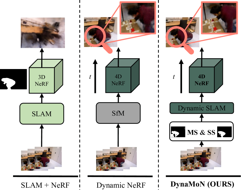
Figure 1: NeRF-SLAM approaches rely on static scenes (left). However, approaches like InstantNGP [12] used for visualization in NeRF-SLAM [3] or Orbeez-SLAM [11] enable masking out dynamic pixels (left). Still when using the masking the scene representation lacks in quality (left). Dynamic NeRF approaches rely on SfM which are offline and sometimes not successful on highly dynamic scenes (center). Considering dynamics already in the SLAM approach (right) enables better camera tracking and enables novel view synthesis with higher quality.

In this paper, we present DynaMoN, a motion-aware camera localization and visualization approach which can handle highly dynamic scenes. We utilize motion and semantic segmentation during our dynamic camera localization process to enable a robust tracking of the camera path in a dynamic environment. We combine our camera localization approach with a dynamic NeRF to enable a decent visualization of novel views of the scenes. To demonstrate our robustness we evaluate our approach on three challenging datasets, namely the dynamic subset of the TUM RGB-D [13] dataset, the BONN RGB-D Dynamic [14] dataset and the DyCheck’s iPhone [15] dataset.

In summary we contribute:

• DynaMoN, a motion-aware fast and robust camera localization approach for dynamic novel view synthesis.

• State-of-the-art camera localization and novel view synthesis results on TUM RGB-D, BONN RGB-D Dynamic and the DyCheck’s iPhone dataset.

II RELATED WORKS

Our approach DynaMoN combines a dynamic NeRF with a fast and robust motion-aware camera localization, thus, our related works are grouped under the topics of camera localization, their employment for novel view synthesis and neural representation for dynamic scenes.

II-A Camera Localization and Scene Dynamics

SfM and SLAM [16, 17, 18, 19] are the two most common approaches for robust camera localization. More specifically, SLAM often targets real-time localization of a camera coupled with mapping. In addition to the visual information, some approaches can utilize additional sensory signals like depth and IMU to further improve the accuracy. A common branch of work employs ORB descriptors to build and track on sparse 3D maps [16, 19, 17].

In addition to classical or partially learnable SLAM approaches, Teed and Deng [18] introduce the end-to-end learnable DROID-SLAM. DROID-SLAM consists of a Dense Bundle Adjustment layer enabling recurrent iterative updates of camera poses and pixel-wise depth.

Initial camera localization approaches rely on static scenes. However, natural scenes are dynamic [20, 21, 22, 23]. To address this, Yu et al. [20] introduce a dynamic SLAM approach building upon ORB-SLAM2 [19]. Their DS-SLAM integrates a semantic segmentation network and a moving consistency check in the tracking process.

Rünz et al. [24] enrich RGB-D SLAM with object-awareness and semantic segmentation capabilities. DynaSLAM [25] combines geometric and deep learning-based segmentation techniques to effectively mask out dynamic objects.

Dai et al. [22] build upon ORB-SLAM2 [19] and introduce the use of semantic segmentation using point correlation to split dynamic and static points. Ye et al. [23] divide the scene representation in a static flow field and a dynamic flow field.

II-B Camera Localization and NeRF

Using the retrieved camera poses, a captured environment can be represented as a 3D scene representation. One possible scene representation is the use of a multilayer perceptron (MLP) [26]. Mildenhall et al. [26] introduce the use of a MLP as neural representation for novel view synthesis, denoted as NeRF. A NeRF relies on accurate camera poses, typically captured with COLMAP [8]. However, this slows down the overall pipeline. An alternative to SfM is the use of SLAM to retrieve the camera poses.

Sucar et al. [27] introduce the use of an MLP as scene representation in a SLAM approach. Building upon the use of a single MLP, Zhu et al. [9] introduce the use of multiple NeRFs in a hierarchical feature grid to learn the camera pose and scene representation. NICER-SLAM [10] introduces a similar approach for RGB input including depth estimation.

Other approaches purely relying on RGB and combining SLAM and NeRF [3, 11] utilize the well-known hash-based InstantNGP [12] for the scene representation. While NeRF-SLAM [3] builds upon an adaption of Droid-SLAM [18], Orbeez-SLAM [11] leverages visual odometry [19].

II-C Neural Representation of Dynamic Scenes

In real-world, scenes are inherently dynamic in contrast to the assumptions of the more common static representation [9, 10, 27, 11, 3, 12, 26]. To represent dynamics in a NeRF, the use of grid structures has been a popular approach [4, 5]. HexPlane [4] utilizes a 4D space-time grid divided into six feature planes. The feature vector is a 4D point in space-time which is projected onto each feature plane. Similarly, Tensor4d [5] builds upon a 4D tensor field using time-aware volumes projected onto nine 2D planes. TiNeuVox [7] represents dynamic scenes using time-aware voxel features and enables faster training.

Optimizing the camera poses and the view synthesis has been explored in static scenes [28, 29, 30, 31, 32] and often improved the novel view synthesis. Liu et al. [33] introduce this optimization to a dynamic NeRF. To model the dynamic scene, they use one static and one dynamic NeRF, where the static NeRF is optimized using the camera poses.

III Method

In our setup we consider our input to be a video captured in a dynamic environment using a moving camera without knowing its poses. This leads to two objectives: first, to estimate the camera poses along the dynamic input, and second, to build a 4D representation enabling novel views using the input images and predicted camera poses.

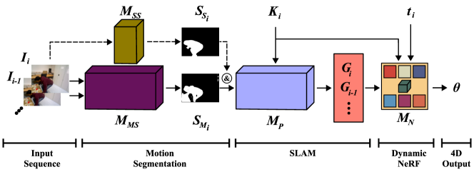
Figure 2: Our DynaMoN architecture. We utilize segmentation ($M_{ss}\rightarrow S_{S_{i}}$) and motion masks ($M_{MS}\rightarrow S_{M_{i}}$) on the input images ($I$) to enable a motion-aware fast and robust camera localization. Based on the predicted camera poses $G_{i},G_{i-1,...}$ and the camera intrinsic ($K_{i}$) we produce a 4D output ($\Theta$) using dynamic NeRF ($M_{N}$).

III-A Camera Localization

Our work builds upon DROID-SLAM [18]. To enhance its capacity of coping with highly dynamic scenes, we take advantage of motion and semantic segmentation, see Figure 2. Our underlying architecture [18] solves a dense bundle adjustment problem in every iteration for a set of keyframes to acquire their corresponding poses G and depths d. It is weighted by the confidences $w_{ij}$ of the optical flow calculation by RAFT [34]:

$$\textbf{E}(\textbf{G},\textbf{d})=\sum_{(i,j)\in\epsilon}\left\|p_{ij}^{*}-\Pi_{C}(G_{ij}\circ\Pi_{C}^{-1}(p_{i},d_{i}))\right\|^{2}_{\Sigma_{ij}},$$ (1)

where $\Sigma_{ij}=diag(w_{ij})$, $p_{ij}^{*}$ is the estimated optical flow, $G_{ij}$ is the motion between the poses $G_{i}$ and $G_{j}$ and $p_{i}$ as well as $d_{i}$ represent the pixel grid and inverse depth map of frame $i$ [18]. $(i,j)\in\epsilon$ means that there exists an edge between the images $i$ and $j$ in the frame graph of the SLAM method, i.e. they have overlapping fields of view. $\circ$ represents the retraction on the SE3 manifold and $\Pi_{C}$ as well as $\Pi_{C}^{-1}$ the projection function from 3D to the image plane and inverse projection function, respectively. The remaining poses that do not belong to keyframes are filled in with a motion-only bundle adjustment in the end. To introduce our proposed masking of dynamics, we set the weight $w_{ij}$ equal to $0$, wherever one of the motion ($M_{MS}$) or the segmentation mask ($M_{SS}$) evaluates to true. Due to the nature of the Mahalanobis distance, potentially dynamic pixels will then not be considered for optimization.

Our semantic segmentation module predicts masks for the predefined classes person, cat and dog, since these appear in the used datasets. We use a pre-trained version of the state-of-the-art semantic segmentation network DeepLabV3 [35] with a ResNet50-backbone [36]. Additionally, we utilize a motion-based filtering of pixels belonging to dynamic objects to enhance the segmentation of dynamics ($M_{MS}$). This enables our approach to deal with a greater variety of dynamics independent of previously known categories. We refine the motion mask and the estimated camera movement between two adjacent frames twice with an incremental increase of the segmentation threshold [37].

III-B Dynamic Scene Representation

While our dynamic camera localization module enables the retrieval of camera poses in dynamic scenes, a 4D scene representation and novel view generation is achieved with dynamic NeRF. To represent a scene in 4D (3D$+t$) we follow the combination of implicit and explicit representation presented by Cao and Johnson [4]. Our NeRF consists of six features planes, each pair for one coordinate axis (e.g. XY, XZ, YT) [4].

The 3D scene is represented as a 4D feature volume $V\in\mathbf{R}^{X\times Y\times Z\times T\times F}$ [4]:

$$\begin{split}\sum_{r=1}^{R_{1}}\mathbf{M}_{r}^{X\times Y}\otimes\mathbf{M}_{r}^{Z\times T}\otimes\mathbf{v}_{r}^{1}&+\sum_{r=1}^{R_{2}}\mathbf{M}_{r}^{X\times Z}\otimes\mathbf{M}_{r}^{Y\times T}\otimes\mathbf{v}_{r}^{2}\\ &+\sum_{r=1}^{R_{3}}\mathbf{M}_{r}^{Y\times Z}\otimes\mathbf{M}_{r}^{X\times T}\otimes\mathbf{v}_{r}^{3},\end{split}$$ (2)

where each $\textbf{M}_{r}^{A\times B}\in\mathbf{R}^{A\times B}$ is one of the six learned feature planes, $\mathbf{v}_{r}^{i}$ are vectors along the $F$ axis and $\otimes$ represents the outer product. Each pair of feature planes (e.g. $\textbf{M}_{r}^{X\times Y},\textbf{M}_{r}^{Z\times T}$) has one spatial and one spatio-temporal plane. Color and density features acquired from the feature planes are fed into tiny MLPs to yield the final density and RGB color values.

To optimize our NeRF module we sample batches of rays $\mathcal{R}$ for which we compute the mean squared error between the rendered RGB values $C$ and the ground truth $\hat{C}$:

$$L_{RGB}=\frac{1}{|\mathcal{R}|}\sum_{r\in\mathcal{R}}\left\|C(r)-\hat{C}(r)\right\|_{2}^{2}.$$ (3)

In addition, we apply the Total Variation (TV) loss [38, 4] as regularization term for the features $x$ of each feature plane. For the multi-spatial planes this results in

$$\begin{split}L_{TV,s}&=\frac{2}{b}\sum_{i,j}(\frac{1}{N}\left(x_{i,j}-x_{i+1,j}\right)^{2}\\ &+\frac{1}{M}\left(x_{i,j}-x_{i,j+1}\right)^{2})\end{split}$$ (4)

and for the spatio-temporal planes in

$$\begin{split}L_{TV,ts}&=\frac{2}{b}\sum_{i,j}(\frac{1}{N}\left(x_{i,j}-x_{i+1,j}\right)^{2}\\ &+\frac{\lambda_{ts}}{M}\left(x_{i,j}-x_{i,j+1}\right)^{2}).\end{split}$$ (5)

Here, $N$ is the total number of differences in the first plane dimension, $M$ is the total number of differences in the second dimension and b is the batch size. In total, $L_{TV,\sigma}$ is the sum of the TV losses over all feature planes for the density and $L_{TV,RGB}$ the same for the color. Thus, the overall loss function for training the NeRF, which is done in a coarse-to-fine manner, is characterized by the following:

$$L_{NeRF}=L_{RGB}+\lambda_{TV}(L_{TV,\sigma}+wL_{TV,RGB}).$$ (6)

TABLE I: Absolute Trajectory Error (RMS) [m] on TUM RGB-D [13].

	Sequences		RGB-D					Monocular
		DVO-SLAM  [39]	ORB-SLAM2 [19]	PointCorr [22]		DytanVO [37]	DeFlowSLAM [23]	DROID-SLAM [18]	OURS (MS&SS)	OURS (MS)
slightly dynamic	fr2/desk-person	0.104	0.006	0.008		1.166	0.013	0.006	0.007	0.006
	fr3/sitting-static	0.012	0.008	0.010		0.016	0.007	0.005	0.005	0.005
	fr3/sitting-xyz	0.242	0.010	0.009		0.260	0.015	0.009	0.010	0.009
	fr3/sitting-rpy	0.176	0.025	0.023		0.046	0.027	0.022	0.024	0.021
	fr3/sitting-halfsphere	0.220	0.025	0.024		0.310	0.025	0.014	0.023	0.019
highly dynamic	fr3/walking-static	0.752	0.408	0.011		0.021	0.007	0.012	0.007	0.014
	fr3/walking-xyz	1.383	0.722	0.087		0.028	0.018	0.016	0.014	0.014
	fr3/walking-rpy	1.292	0.805	0.161		0.155	0.057	0.040	0.031	0.039
	fr3/walking-halfsphere	1.014	0.723	0.035		0.385	0.420	0.022	0.019	0.020
	Mean/Max	0.577/1.383	0.304/0.805	0.041/0.161		0.265/1.166	0.065/0.420	0.016/0.040	0.016/0.031	0.016/0.039

TABLE II: Absolute Trajectory Error (RMS) [m] on DyCheck’s iPhone [15]. The - denotes that the camera pose could not be regressed.

Sequences	COLMAP [8]		DROID-SLAM [18]	OURS	OURS
				(MS&SS)	(MS)
Apple	-		0.004	0.007	0.004
Backpack	-		0.008	0.006	0.008
Block	-		0.052	0.005	0.005
Creeper	0.031		0.004	0.004	0.004
Handwavy	-		0.002	0.001	0.001
Haru	-		0.008	0.007	0.008
Mochi	-		0.002	0.002	0.002
Paper Windmill	0.012		0.002	0.002	0.002
Pillow	-		0.058	0.020	0.023
Space Out	0.057		0.008	0.008	0.008
Spin	0.015		0.005	0.004	0.004
Sriracha	-		0.002	0.002	0.002
Teddy	-		0.015	0.011	0.010
Wheel	-		0.005	0.004	0.063
Mean/Max	-		0.013/0.058	0.006/0.020	0.010/0.063

IV Evaluation

DynaMoN is assessed on three tough datasets, examining camera localization and novel view synthesis quality.

TABLE III: Absolute Trajectory Error (RMS) [m] on BONN RGB-D [14]

Sequences			RGB-D				Monocular
	ReFusion [14]	StaticFusion [40]	DynaSLAM (G) [25]	DynaSLAM (N+G) [25]		DROID-SLAM [18]	OURS (MS&SS)	OURS (MS)
balloon	0.175	0.233	0.050	0.030		0.075	0.028	0.068
balloon2	0.254	0.293	0.142	0.029		0.041	0.027	0.038
balloon_tracking	0.302	0.221	0.156	0.049		0.035	0.034	0.036
balloon_tracking2	0.322	0.366	0.192	0.035		0.026	0.032	0.028
crowd	0.204	3.586	1.065	0.016		0.052	0.035	0.061
crowd2	0.155	0.215	1.217	0.031		0.065	0.028	0.056
crowd3	0.137	0.168	0.835	0.038		0.046	0.032	0.055
kidnapping_box	0.148	0.336	0.026	0.029		0.020	0.021	0.020
kidnapping_box2	0.161	0.263	0.033	0.035		0.017	0.017	0.017
moving_no_box	0.071	0.141	0.317	0.232		0.023	0.013	0.014
moving_no_box2	0.179	0.364	0.052	0.039		0.040	0.027	0.026
moving_o_box	0.343	0.331	0.544	0.044		0.177	0.152	0.167
moving_o_box2	0.528	0.309	0.589	0.263		0.236	0.175	0.176
person_tracking	0.289	0.484	0.714	0.061		0.043	0.148	0.024
person_tracking2	0.463	0.626	0.817	0.078		0.054	0.022	0.035
placing_no_box	0.106	0.125	0.645	0.575		0.078	0.021	0.018
placing_no_box2	0.141	0.177	0.027	0.021		0.030	0.020	0.020
placing_no_box3	0.174	0.256	0.327	0.058		0.025	0.022	0.022
placing_o_box	0.571	0.330	0.267	0.255		0.127	0.172	0.117
removing_no_box	0.041	0.136	0.016	0.016		0.016	0.015	0.015
removing_no_box2	0.111	0.129	0.022	0.021		0.020	0.019	0.021
removing_o_box	0.222	0.334	0.362	0.291		0.189	0.177	0.181
synchronous	0.441	0.446	0.977	0.015		0.006	0.007	0.006
synchronous2	0.022	0.027	0.887	0.009		0.012	0.006	0.011
Mean/Max	0.232/0.571	0.412/3.586	0.428/1.217	0.095/0.575		0.061/0.236	0.052/0.177	0.051/0.181

IV-A Datasets

To assess DynaMoN, we compare both the camera localization and the novel view synthesis part with state-of-the-art approaches on three challenging datasets.

TUM RGB-D - Dynamic subset [13]: The TUM RGB-D dataset has a resolution of $640\times 480$. While the dataset mainly focuses on static parts, five sequences were rated slightly dynamic and four highly dynamic.

BONN RGB-D Dynamic [14]: The BONN RGB-D Dynamic consists of 24 dynamic sequences and 2 static sequences. The number of recordings per scene varies. The images have a resolution of $640\times 480$.

DyCheck’s iPhone [15]: The iPhone dataset consists of 14 scenes, seven captured with multi cameras and another seven scenes captured with a single camera. The sequences are taken with an iPhone including a lidar scanner for depth. The resolution of the images is $720\times 960$.

For the novel view synthesis results we use every 8th frame of the TUM RGB-D dataset and BONN RGB-D Dynamic dataset for testing. On the iPhone dataset we follow the official evaluation split.

IV-B Implementation Details

We implemented our approach in Python using PyTorch [41] as the deep learning framework. While we use the reported image sizes for the novel view synthesis experiments, we use half of the resolution for the camera localization to be consistent with existent trajectory evaluations of [18]. For our motion mask module we introduce a threshold to avoid false positives. We set the initial threshold to 0.95 and increase it to 0.98 throughout the motion mask refinement. For cases where the camera motion is higher than in the training sequences, the motion segmentation module results in an increase of false positives, as a counter-measurement we introduce a thresholding for the number of pixels that contain motion. Consequently, masks exceeding this threshold are discarded. This ensures that there is always enough pixels for the dense bundle adjustment.

For the loss functions we set $w$ for $L_{NeRF}$ to 0.1, $\lambda_{ts}$ to 20 and $\lambda_{TV}$ initially to 0.005.

To compare our camera pose retrieval with the classic way of using COLMAP, we followed the implementation of InstantNGP [12] to retrieve the COLMAP ground truth.

Besides the COLMAP comparison, we compare our approach with RoDynRF [33]. For the TUM RGB-D dataset, we train their approach on a NVIDIA RTX 3090 with 24GB of VRAM. We follow their training guideline and do not employ prior pose initialization.

TABLE IV: Novel view synthesis results on TUM RGB-D [13]. The - denotes that the camera pose could not be regressed.

Sequences		PSNR$\uparrow$/SSIM$\uparrow$
		RoDynRF [33]	Ours (COLMAP)	Ours (SLAM)
slightly dynamic	fr2/desk-person	5.87 / 0.018	-	23.04 / 0.680
	fr3/sitting-static	9.43 / 0.151	-	28.55 / 0.899
	fr3/sitting-xyz	11.26 / 0.213	19.98 / 0.589	25.90 / 0.848
	fr3/sitting-rpy	8.94 / 0.197	16.63 / 0.472	25.76 / 0.843
	fr3/sitting-halfsphere	8.07 / 0.216	24.25 / 0.793	24.05 / 0.792
highly dynamic	fr3/walking-static	5.99 / 0.009	20.27 / 0.650	25.84 / 0.849
	fr3/walking-xyz	10.07 / 0.183	-	24.05 / 0.797
	fr3/walking-rpy	10.08 / 0.207	-	24.18 / 0.790
	fr3/walking-halfsphere	9.60 / 0.253	22.01 / 0.692	24.05 / 0.781
Mean		8.81 / 0.161	-	25.05 / 0.809

IV-C Evaluation Metrics

To evaluate our approach, we consider two aspects. First, we consider the translational trajectory error using RMS in meters. Second, we analyze the rendering quality of the novel dynamic views by reporting PSNR and SSIM [42] values.

TABLE V: Novel view synthesis results on BONN RGB-D Dynamic [14]. The - denotes that the camera pose could not be regressed.

Sequences	PSNR$\uparrow$/SSIM$\uparrow$
	Ours (COLMAP)	Ours (SLAM)
balloon	-	29.83 / 0.868
balloon2	-	27.61 / 0.841
balloon_tracking	-	29.27 / 0.847
balloon_tracking2	-	29.68 / 0.860
crowd	-	27.92 / 0.831
crowd2	-	26.68 / 0.825
crowd3	-	26.57 / 0.815
kidnapping_box	-	30.43 / 0.870
kidnapping_box2	30.87 / 0.881	30.28 / 0.860
moving_no_box	30.67 / 0.881	30.32 / 0.866
moving_no_box2	31.14 / 0.890	30.57 / 0.874
moving_o_box	29.21 / 0.889	30.26 / 0.884
moving_o_box2	-	29.82 / 0.875
person_tracking	26.57 / 0.808	27.78 / 0.843
person_tracking2	-	27.47 / 0.837
placing_no_box	25.73 / 0.780	30.94 / 0.869
placing_no_box2	-	31.18 / 0.885
placing_no_box3	-	30.79 / 0.879
placing_o_box	-	30.42 / 0.886
removing_no_box	-	30.66 / 0.879
removing_no_box2	31.13 / 0.887	30.73 / 0.871
removing_o_box	31.13 / 0.887	30.30 / 0.880
synchronous	-	28.42 / 0.835
synchronous2	-	28.85 / 0.887
Mean	-	29.45 / 0.861

IV-D Camera Localization Quality

Our results on all datasets show a lower trajectory error compared to the state-of-the-art approaches. For the TUM RGB-D dataset, the camera trajectory error is denoted in Table I. We compare RGB-D-based and monocular SLAM approaches with our proposed camera retrieval method using only motion masks (MS) as well as using motion and semantic segmentation masks in combination (MS&SS). For the mean value of the trajectory error, our approach performs equally compared to DROID-SLAM. However, for the maximum error value our approach performs best among the compared results.

Additionally, we evaluate our approach on the BONN RGB-D Dynamic dataset in Table III. This dataset contains more dynamic scenes compared to the dynamic sequences of the TUM RGB-D dataset. On this dataset, our approach outperforms the state-of-the-art approaches in terms of mean and max trajectory error.

Testing our approach on camera localization datasets we compare our method with DROID-SLAM and COLMAP on the DyCheck’s iPhone dataset [15], see Table II. DynaMoN outperforms DROID-SLAM on the iPhone dataset. COLMAP fails to generate camera poses for the majority of the sequences.

TABLE VI: Novel view synthesis results on the iPhone dataset [15]

Sequences	PSNR$\uparrow$/SSIM$\uparrow$
	RoDynRF [33]	Ours (SLAM)
Apple	18.73 / 0.722	15.92 / 0.694
Block	18.73 / 0.634	17.17 / 0.655
Paper Windmill	16.71 / 0.321	18.28 / 0.380
Space Out	18.56 / 0.594	17.08 / 0.590
Spin	17.41 / 0.484	15.94 / 0.544
Teddy	14.33 / 0.536	13.56 / 0.544
Wheel	15.20 / 0.449	14.81 / 0.532
Mean	17.09 / 0.534	16.11 / 0.563

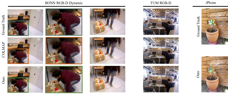
Figure 3: Novel views from DynaMoN (Ours) compared to the Ground Truth and COLMAP-based dynamic NeRF on the BONN RGB-D dynamic dataset (left). On the TUM RGB-D dataset we compare DynaMoN (Ours) and the ground truth.

IV-E Novel View Synthesis Quality

To evaluate our approach from a NeRF perspective we consider two aspects. First, the classic way of generating camera ground truth when using NeRF is the use of COLMAP. Thus, we compare our DynaMoN using the same dynamic NeRF but with camera poses from COLMAP. Second, we compare our approach with RoDynRF [33] which regresses the camera pose along with a dynamic NeRF.

The results for the TUM RGB-D dataset, denoted in Table IV show that DynaMoN leads to a higher novel view synthesis quality compared to RoDynRF or when using the classic COLMAP for the camera poses. Examples of our renderings can be found in Fig. 3.

On the BONN RGB-D dataset, see Table V, COLMAP is challenged on several sequences. First, our DynaMoN can retrieve all camera poses, see Table III, and second, our approach performs well on all sequences of the BONN RGB-D dataset for the novel view synthesis. Examples can be seen in Fig. 3. However, if COLMAP was successful, the accurate camera poses also lead to decent novel view synthesis results.

In addition to the SLAM datasets, we compare our approach with the most similar NeRF approach RoDynRF [33] on the multi-camera scenes of the DyCheck’s iPhone dataset, see Table VI. We achieve similar but slightly worse performance on this dataset in PSNR. However, for SSIM our approach shows better results.

V DISCUSSION

In comparison to more sparse reconstructions, our approach addresses camera localization and novel view synthesis in combination. While this leads to more pleasing 3D visualizations and novel views, the computing time is higher compared to traditional camera localization and 3D representation methods.

Our evaluation considers two aspects, the robustness of the camera pose estimation and the novel view synthesis results. For the camera pose estimation, our approach shows an improved performance compared to the state-of-the-art approaches. Furthermore, our used motion masks already provide an improved performance. However, on scenes with large motions the combination with semantic segmentation masks provide an improved camera localization result. Moreover, we demonstrate that our approach also achieve a robust performance on scenes with less camera motion, normally used for novel view synthesis, see Table II.

According to the results in Table IV, existing camera regression and novel view synthesis results are challenged by more dynamic camera motions and dynamic scenes.

Although our approach has demonstrated competitive results on the TUM RGB-D and BONN RGB-D datasets, it faced challenges when applied to the multi-camera iPhone dataset due to its narrower field of view. Additionally, on the BONN RGB-D Dynamic dataset, our approach struggled with handling strong light influences near the camera, as illustrated in Fig. 4. Future work could focus on enhancing motion mask prediction by eliminating the need for predefined classes.

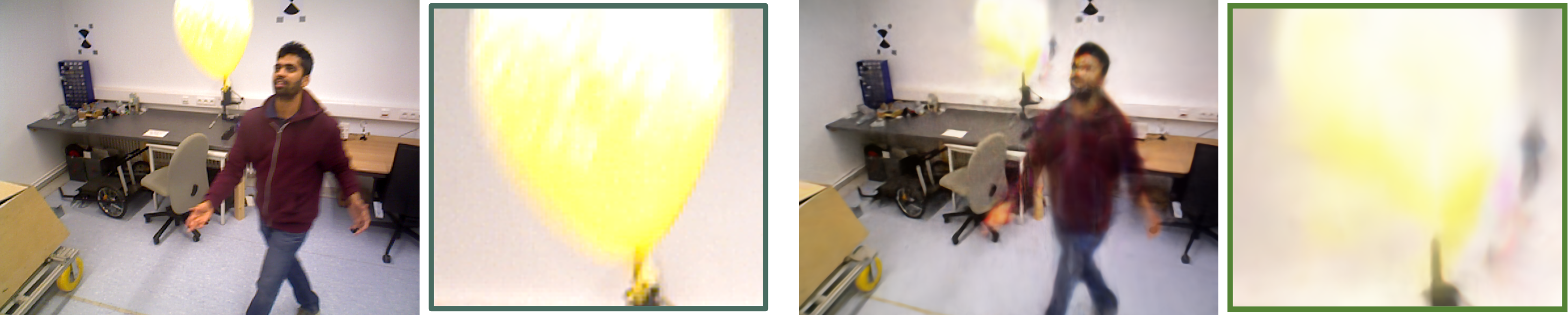
Figure 4: Failure cases. Our DynaMoN (center and right bottom) is challenged by dynamics with a high light influence.

VI CONCLUSION

We present DynaMoN, a motion aware fast and robust camera localization approach for novel view synthesis. DynaMoN can handle not only the motion of known objects using semantic segmentation masks but also that of unknown objects using a motion segmentation mask. Furthermore, it retrieves the camera poses faster and more robust compared to classical SfM approaches enabling a more accurate 4D scene representation. Compared to the state-of-the-art, DynaMoN outperforms other dynamic camera localization approaches and shows better results for novel view synthesis.

References

- [1] M. Broxton, J. Flynn, R. Overbeck, D. Erickson, P. Hedman, M. Duvall, J. Dourgarian, J. Busch, M. Whalen, and P. Debevec, “Immersive light field video with a layered mesh representation,” ACM Trans. Graph., vol. 39, no. 4, aug 2020. [Online]. Available: https://doi.org/10.1145/3386569.3392485
- [2] S. Orts-Escolano, C. Rhemann, S. Fanello, W. Chang, A. Kowdle, Y. Degtyarev, D. Kim, P. L. Davidson, S. Khamis, M. Dou et al., “Holoportation: Virtual 3d teleportation in real-time,” in Proceedings of the 29th annual symposium on user interface software and technology, 2016, pp. 741–754.
- [3] A. Rosinol, J. J. Leonard, and L. Carlone, “Nerf-slam: Real-time dense monocular slam with neural radiance fields,” arXiv preprint arXiv:2210.13641, 2022.
- [4] A. Cao and J. Johnson, “Hexplane: A fast representation for dynamic scenes,” in Proceedings of the IEEE/CVF Conference on Computer Vision and Pattern Recognition, 2023, pp. 130–141.
- [5] R. Shao, Z. Zheng, H. Tu, B. Liu, H. Zhang, and Y. Liu, “Tensor4d: Efficient neural 4d decomposition for high-fidelity dynamic reconstruction and rendering,” in Proceedings of the IEEE/CVF Conference on Computer Vision and Pattern Recognition, 2023, pp. 16 632–16 642.
- [6] L. Song, A. Chen, Z. Li, Z. Chen, L. Chen, J. Yuan, Y. Xu, and A. Geiger, “Nerfplayer: A streamable dynamic scene representation with decomposed neural radiance fields,” IEEE Transactions on Visualization and Computer Graphics, pp. 2732–2742, 2023.
- [7] J. Fang, T. Yi, X. Wang, L. Xie, X. Zhang, W. Liu, M. Nießner, and Q. Tian, “Fast dynamic radiance fields with time-aware neural voxels,” in SIGGRAPH Asia 2022 Conference Papers, 2022.
- [8] J. L. Schonberger and J.-M. Frahm, “Structure-from-motion revisited,” in Proceedings of the IEEE conference on computer vision and pattern recognition, 2016, pp. 4104–4113.
- [9] Z. Zhu, S. Peng, V. Larsson, W. Xu, H. Bao, Z. Cui, M. R. Oswald, and M. Pollefeys, “Nice-slam: Neural implicit scalable encoding for slam,” in Proceedings of the IEEE/CVF Conference on Computer Vision and Pattern Recognition, 2022, pp. 12 786–12 796.
- [10] Z. Zhu, S. Peng, V. Larsson, Z. Cui, M. R. Oswald, A. Geiger, and M. Pollefeys, “Nicer-slam: Neural implicit scene encoding for rgb slam,” arXiv preprint arXiv:2302.03594, 2023.
- [11] C.-M. Chung, Y.-C. Tseng, Y.-C. Hsu, X.-Q. Shi, Y.-H. Hua, J.-F. Yeh, W.-C. Chen, Y.-T. Chen, and W. H. Hsu, “Orbeez-slam: A real-time monocular visual slam with orb features and nerf-realized mapping,” in 2023 IEEE International Conference on Robotics and Automation (ICRA). IEEE, 2023, pp. 9400–9406.
- [12] T. Müller, A. Evans, C. Schied, and A. Keller, “Instant neural graphics primitives with a multiresolution hash encoding,” ACM Transactions on Graphics (ToG), vol. 41, no. 4, pp. 1–15, 2022.
- [13] J. Sturm, N. Engelhard, F. Endres, W. Burgard, and D. Cremers, “A benchmark for the evaluation of rgb-d slam systems,” in Proc. of the International Conference on Intelligent Robot Systems (IROS), Oct. 2012.
- [14] E. Palazzolo, J. Behley, P. Lottes, P. Giguère, and C. Stachniss, “ReFusion: 3D Reconstruction in Dynamic Environments for RGB-D Cameras Exploiting Residuals,” in 2019 IEEE/RSJ International Conference on Intelligent Robots and Systems (IROS). IEEE, 2019, pp. 7855–7862.
- [15] H. Gao, R. Li, S. Tulsiani, B. Russell, and A. Kanazawa, “Monocular dynamic view synthesis: A reality check,” Advances in Neural Information Processing Systems, vol. 35, pp. 33 768–33 780, 2022.
- [16] R. Mur-Artal, J. M. M. Montiel, and J. D. Tardos, “Orb-slam: a versatile and accurate monocular slam system,” IEEE transactions on robotics, vol. 31, no. 5, pp. 1147–1163, 2015.
- [17] C. Campos, R. Elvira, J. J. G. Rodríguez, J. M. Montiel, and J. D. Tardós, “Orb-slam3: An accurate open-source library for visual, visual–inertial, and multimap slam,” IEEE Transactions on Robotics, vol. 37, no. 6, pp. 1874–1890, 2021.
- [18] Z. Teed and J. Deng, “Droid-slam: Deep visual slam for monocular, stereo, and rgb-d cameras,” Advances in neural information processing systems, vol. 34, pp. 16 558–16 569, 2021.
- [19] R. Mur-Artal and J. D. Tardós, “Orb-slam2: An open-source slam system for monocular, stereo, and rgb-d cameras,” IEEE transactions on robotics, vol. 33, no. 5, pp. 1255–1262, 2017.
- [20] C. Yu, Z. Liu, X.-J. Liu, F. Xie, Y. Yang, Q. Wei, and Q. Fei, “Ds-slam: A semantic visual slam towards dynamic environments,” in 2018 IEEE/RSJ international conference on intelligent robots and systems (IROS). IEEE, 2018, pp. 1168–1174.
- [21] M. Henein, J. Zhang, R. Mahony, and V. Ila, “Dynamic slam: The need for speed,” in 2020 IEEE International Conference on Robotics and Automation (ICRA). IEEE, 2020, pp. 2123–2129.
- [22] W. Dai, Y. Zhang, P. Li, Z. Fang, and S. Scherer, “Rgb-d slam in dynamic environments using point correlations,” IEEE Transactions on Pattern Analysis and Machine Intelligence, vol. 44, no. 1, pp. 373–389, 2020.
- [23] W. Ye, X. Yu, X. Lan, Y. Ming, J. Li, H. Bao, Z. Cui, and G. Zhang, “Deflowslam: Self-supervised scene motion decomposition for dynamic dense slam,” arXiv preprint arXiv:2207.08794, 2022.
- [24] M. Runz, M. Buffier, and L. Agapito, “Maskfusion: Real-time recognition, tracking and reconstruction of multiple moving objects,” in 2018 IEEE International Symposium on Mixed and Augmented Reality (ISMAR). IEEE, 2018, pp. 10–20.
- [25] B. Bescos, J. M. Fácil, J. Civera, and J. Neira, “Dynaslam: Tracking, mapping, and inpainting in dynamic scenes,” IEEE Robotics and Automation Letters, vol. 3, no. 4, pp. 4076–4083, 2018.
- [26] B. Mildenhall, P. P. Srinivasan, M. Tancik, J. T. Barron, R. Ramamoorthi, and R. Ng, “Nerf: Representing Scenes as Neural Radiance Fields for View Synthesis,” in European Conference on Computer Vision. Springer, 2020, pp. 405–421.
- [27] E. Sucar, S. Liu, J. Ortiz, and A. J. Davison, “imap: Implicit mapping and positioning in real-time,” in Proceedings of the IEEE/CVF International Conference on Computer Vision, 2021, pp. 6229–6238.
- [28] Z. Wang, S. Wu, W. Xie, M. Chen, and V. A. Prisacariu, “NeRF–: Neural radiance fields without known camera parameters,” arXiv preprint arXiv:2102.07064, 2021.
- [29] Q. Meng, A. Chen, H. Luo, M. Wu, H. Su, L. Xu, X. He, and J. Yu, “GNeRF: GAN-Based Neural Radiance Field Without Posed Camera,” in Proceedings of the IEEE/CVF International Conference on Computer Vision (ICCV), Oct. 2021, pp. 6351–6361.
- [30] L. Yen-Chen, P. Florence, J. T. Barron, A. Rodriguez, P. Isola, and T.-Y. Lin, “iNeRF: Inverting Neural Radiance Fields for Pose Estimation,” in 2021 IEEE/RSJ International Conference on Intelligent Robots and Systems (IROS), 2021, pp. 1323–1330.
- [31] W. Bian, Z. Wang, K. Li, J. Bian, and V. A. Prisacariu, “NoPe-NeRF: Optimising Neural Radiance Field with No Pose Prior,” in CVPR.
- [32] H. Schieber, F. Deuser, B. Egger, N. Oswald, and D. Roth, “Nerftrinsic four: An end-to-end trainable nerf jointly optimizing diverse intrinsic and extrinsic camera parameters,” 2023.
- [33] Y.-L. Liu, C. Gao, A. Meuleman, H.-Y. Tseng, A. Saraf, C. Kim, Y.-Y. Chuang, J. Kopf, and J.-B. Huang, “Robust dynamic radiance fields,” in Proceedings of the IEEE/CVF Conference on Computer Vision and Pattern Recognition, 2023, pp. 13–23.
- [34] Z. Teed and J. Deng, “Raft: Recurrent all-pairs field transforms for optical flow,” in Computer Vision–ECCV 2020: 16th European Conference, Glasgow, UK, August 23–28, 2020, Proceedings, Part II 16. Springer, 2020, pp. 402–419.
- [35] L.-C. Chen, G. Papandreou, F. Schroff, and H. Adam, “Rethinking atrous convolution for semantic image segmentation,” arXiv preprint arXiv:1706.05587, 2017.
- [36] K. He, X. Zhang, S. Ren, and J. Sun, “Deep residual learning for image recognition,” in Proceedings of the IEEE conference on computer vision and pattern recognition, 2016, pp. 770–778.
- [37] S. Shen, Y. Cai, W. Wang, and S. Scherer, “Dytanvo: Joint refinement of visual odometry and motion segmentation in dynamic environments,” in 2023 IEEE International Conference on Robotics and Automation (ICRA). IEEE, 2023, pp. 4048–4055.
- [38] A. Chen, Z. Xu, A. Geiger, J. Yu, and H. Su, “Tensorf: Tensorial radiance fields,” in European Conference on Computer Vision. Springer, 2022, pp. 333–350.
- [39] C. Kerl, J. Sturm, and D. Cremers, “Robust odometry estimation for rgb-d cameras,” in 2013 IEEE international conference on robotics and automation. IEEE, 2013, pp. 3748–3754.
- [40] R. Scona, M. Jaimez, Y. R. Petillot, M. Fallon, and D. Cremers, “Staticfusion: Background reconstruction for dense rgb-d slam in dynamic environments,” in 2018 IEEE international conference on robotics and automation (ICRA). IEEE, 2018, pp. 3849–3856.
- [41] A. Paszke, S. Gross, S. Chintala, G. Chanan, E. Yang, Z. DeVito, Z. Lin, A. Desmaison, L. Antiga, and A. Lerer, “Automatic differentiation in pytorch,” 2017.
- [42] Z. Wang, A. C. Bovik, H. R. Sheikh, and E. P. Simoncelli, “Image quality assessment: from error visibility to structural similarity,” IEEE transactions on image processing, vol. 13, no. 4, pp. 600–612, 2004, publisher: IEEE.