DOMAIN: MilDly COnservative Model-BAsed OfflINe Reinforcement Learning

Abstract

Model-based reinforcement learning (RL), which learns environment model from offline dataset and generates more out-of-distribution model data, has become an effective approach to the problem of distribution shift in offline RL. Due to the gap between the learned and actual environment, conservatism should be incorporated into the algorithm to balance accurate offline data and imprecise model data. The conservatism of current algorithms mostly relies on model uncertainty estimation. However, uncertainty estimation is unreliable and leads to poor performance in certain scenarios, and the previous methods ignore differences between the model data, which brings great conservatism. Therefore, this paper proposes a milDly cOnservative Model-bAsed offlINe RL algorithm (DOMAIN) without estimating model uncertainty to address the above issues. DOMAIN introduces adaptive sampling distribution of model samples, which can adaptively adjust the model data penalty. In this paper, we theoretically demonstrate that the Q value learned by the DOMAIN outside the region is a lower bound of the true Q value, the DOMAIN is less conservative than previous model-based offline RL algorithms and has the guarantee of security policy improvement. The results of extensive experiments show that DOMAIN outperforms prior RL algorithms on the D4RL dataset benchmark, and achieves better performance than other RL algorithms on tasks that require generalization.

I Introduction

Reinforcement learning (RL) aims to maximize user-defined rewards and acquire optimal behavioral skill. Since the 1970s, RL research has attracted widespread attention, and the advent of deep neural networks has greatly facilitated its development. Today, RL has been applied in various fields, including robot control [1, 2], autonomous driving [3], recommendation systems [4], and resource scheduling [5].

The paradigm of online RL involves an agent interacting with environment directly through trial-and-error[6]. However, online RL suffers from low sampling efficiency and high costs, making it impractical in certain scenarios [7]. For instance, in situations such as surgery and autonomous driving, real-time interaction between the agent and the environment may pose a threat to human safety. Since the robot may damage its components or surrounding objects, the cost of trial-and-error can be prohibitive in robot control [8]. Offline RL can effectively address these issues by learning policy from a static dataset without direct interaction with the environment.

Offline RL faces a significant challenge due to distribution shift, which is caused by differences between the policies in offline dataset and those learned by the agent. The selection of out-of-distribution (OOD) actions introduces extrapolation errors that may lead to unstable training of the agent [9]. To address the above issue, two types of methods have been developed: policy constraints [10, 11, 12] and value penalization [13, 14]. The goal of the above methods is to minimize the discrepancy between the learned policy and that in the dataset. While they achieve remarkable performance, these methods fail to consider the effects of OOD actions, hampering the exploration and performance improvement. In contrast, Lyu et al. [15] proved that the agent performance can be effectively enhanced by exploring OOD region.

The aforementioned offline RL methods are model-free, which constrains exploration in OOD region, hindering performance improvements for agents. In contrast, model-based offline RL enables agents to continually interact with a trained environment model, generating data with broader coverage, thereby enhancing exploration in OOD region [16]. Moreover, agents acquire imaginative abilities through environmental modeling, enabling effective planning and improving control efficacy [17, 18].

Due to the uncertainty of environment model, exploration by agents also carries risks. Therefore, it is critical to strike a balance between return and risk. Scholars [19, 20] have proposed various algorithms that estimate model uncertainty or penalize state-action pairs with high uncertainty during training to incorporate conservatism. Experimental results have shown that model-based offline RL methods outperform most current model-free offline RL methods. However, measuring model uncertainty through neural networks results in prediction errors and low reliability. To address this issue, Yu et al. [21] proposed the COMBO algorithm based on CQL [13], which regularizes model data to suppress unreliable data and enhance reliable offline data. Rigter et al. [24] and Bhardwaj et al. [25] used an adversarial training framework, forcing the agent to act conservatively in OOD region.

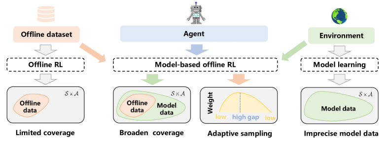
Figure 1: Illustration of mildly conservative model-based offline RL framework. This method integrates offline RL with model-based RL, aiming to leverage the model to broaden data coverage. The key lies in designing a model data adaptive sampling distribution based on the magnitude of model errors, enabling adaptive adjustment of model data penalty.

However, the above methods ignore differences between the model data and are overly conservative. Therefore, we design an adaptive sampling distribution of model data, and propose a mildly conservative model-based offline RL algorithm (DOMAIN) without estimating model uncertainty (as illustrated in Fig. 1). Here, the mildly conservatism is reflected in the following: higher exploration in OOD region and better performance of the agent. This algorithm imposes heavier penalties on model data with high errors while reducing the penalty for accurate model data to alleviate conservatism. Our main contributions are summarized as follows:

1. A new model-based offline RL method is proposed that adaptively adjusts the model data penalty, named DOMAIN, where the adaptive sampling distribution of model samples is designed. To our best knowledge, this is the first to incorporate adaptive sampling distribution to conservative value estimation in model-based offline RL.

2. Theoretical analyses demonstrate that the value function learned by the DOMAIN in the OOD region is a lower bound of the true value function, the DOMAIN is less conservative than previous offline model-based RL algorithms, and DOMAIN has a safety policy improvement guarantee.

3. Extensive experiments indicate that DOMAIN outperforms prior RL algorithms on the D4RL dataset benchmark, and achieves the best performance than other RL algorithms on tasks that require generalization.

The framework of this paper is as follows: Section 2 introduces the fundamental theory of RL. Section 3 shows the framework and implementation details of the DOMAIN algorithm. Section 4 gives some relevant theoretical analysis. Section 5 presents the algorithm performance on D4RL and generalization tasks. Finally, Section 6 summarizes the entire work and provides directions for future research.

II Preliminaries and related works

II-A Reinforcement Learning

The framework of RL is based on the Markov Decision Process (MDP) $\mathcal{M}=\left(\mathcal{S},\mathcal{A},r,T_{\mathcal{M}},\rho_{0},\gamma\right)$, where $\mathcal{S}$ is the set of states, $\mathcal{A}$ is the set of actions, $r(s,a)$ is the reward function, $T_{\mathcal{M}}\left(s^{\prime}\mid s,a\right)$ represents the dynamic system under $\mathcal{M}$, $\rho_{0}$ is the initial state distribution, and $\gamma\in(0,1)$ is the discount factor [8]. The goal of RL is to learn a policy that maximizes the cumulative reward $J(\mathcal{M},\pi)=\mathbb{E}_{(s,a)\sim d_{\mathcal{M}}^{\pi}(s,a)}[r(s,a)]/1-\gamma$, where $d_{\mathcal{M}}^{\pi}(s,a)=d_{\mathcal{M}}^{\pi}(s)\pi(a\mid s)$ is the marginal distribution of states and actions under the learned policy $\pi$, and $d_{\mathcal{M}}^{\pi}(s)$ is the discounted marginal state distribution under the learned policy $\pi$.

Considering the Bellman operator $\mathcal{T}^{\pi}Q(s,a):=r(s,a)+\gamma\mathbb{E}_{s^{\prime}\sim T_{\mathcal{M}}\left(s^{\prime}\mid s,a\right),a^{\prime}\sim\pi\left(\cdot\mid s^{\prime}\right)}\left[Q^{\pi}\left(s^{\prime},a^{\prime}\right)\right]$, its sample-based counterpart is $\hat{\mathcal{T}}^{\pi}Q(s,a):=r(s,a)+\gamma Q\left(s^{\prime},a^{\prime}\right)$[21]. The Actor-Critic algorithm minimizes the Bellman error to learn the $Q$-function and maximizes the $Q$-function to optimize the policy $\pi$. The formulas are expressed as follows:

$$\hat{Q}\leftarrow\arg\min_{Q}\mathbb{E}_{s,a,s^{\prime}\sim\mathcal{D}}\left[\left(Q(s,a)-\hat{\mathcal{T}}^{\pi}\hat{Q}(s,a)\right)^{2}\right]$$ (1)

$$\hat{\pi}\leftarrow\arg\max_{\pi}\mathbb{E}_{s\sim\mathcal{D},a\sim\pi}[\hat{Q}(s,a)]$$

where $\mathcal{D}$ can be a fixed offline dataset or replay buffer generated by the current policy $\hat{\pi}$ interacting with the environment.

II-B Offline RL

The goal of offline RL is to learn a policy $\pi_{\theta}(\cdot\mid s)$ from an offline dataset $\mathcal{D}=\left\{\left(s_{i},a_{i},r_{i},s_{i}^{\prime}\right)\right\}_{i=1}^{n}$ without interacting with the environment, to maximize the expected discounted reward. However, there exists the distribution shift between the learned policy $\pi_{\theta}(\cdot\mid s)$ and the behavioral policy $\pi_{b}(\cdot\mid s)$ of the dataset, leading to unstable training of the agent [8]. To alleviate this issue, previous studies [10, 11, 12, 13, 14] have introduced regularization on the value function of OOD actions to reduce the probability of selecting OOD actions. Here primarily focuses on CQL[13]. The formulas for policy improvement and policy evaluation are as follows:

$$\hat{Q}\leftarrow \arg\min_{Q}\frac{1}{2}\mathbb{E}_{s,a,s^{\prime}\sim\mathcal{D}}\left[\left(Q(s,a)-\hat{\mathcal{T}}^{\pi}\hat{Q}(s,a)\right)^{2}\right]$$ (2)

$$+\beta\bigg{\{}\mathbb{E}_{s\sim\mathcal{D},a\sim\mu(\cdot\mid s)}\left[Q(s,a)\right]-\mathbb{E}_{s,a\sim\mathcal{D}}\left[Q(s,a)\right]\bigg{\}}$$

$$\hat{\pi}\leftarrow \arg\max_{\pi}\mathbb{E}_{s\sim\mathcal{D},a\sim\pi_{k}}[\hat{Q}(s,a)]$$

where $\beta$ represents the regularization coefficient, $\mu(\cdot\mid s)$ denotes the distribution from which actions are sampled, which can be a uniform distribution or a learned policy. CQL effectively penalizes the $Q$-values in the OOD region, providing a conservative estimate of the value function and alleviating the challenges of overestimation and distribution shift.

II-C Model-based Offline RL

Model-based offline RL refers to training an environment model $\hat{T}_{\phi}\left(s^{\prime},r\mid s,a\right)$ using the offline dataset, where the model is typically parameterized as gaussian distribution $\hat{T}_{\phi}(s^{\prime},r\mid s,a)=\mathcal{N}[\mu_{\phi}(s,a),\Sigma_{\phi}(s,a)]$. The loss function for training the environment model employs maximum likelihood estimation as: $\mathcal{L}_{\mathcal{M}}(\phi)=-\mathbb{E}_{\left(s,a,r,s^{\prime}\right)\sim\mathcal{D}}[\log\hat{T}_{\phi}(s^{\prime},r\mid s,a)]$. With this learned model, an estimated MDP $\hat{\mathcal{M}}$ can be obtained. Subsequently, the agent interacts with the learned policy $\hat{\pi}$ and the environment model $\hat{T}_{\phi}$ to generate model data $\mathcal{D}_{\text{model }}$ through $H$-step rollouts. The policy learning is then performed using the combined dataset $\mathcal{D}_{\text{offline }}\cup\mathcal{D}_{\text{model }}$, where the data is sampled from model data $\mathcal{D}_{\text{model }}$ with the probability $f,f\in[0,1]$, and from the offline data $\mathcal{D}_{\text{offline }}$ with the probability $1-f$.

However, offline dataset fails to cover the entire state-action space, resulting in disparities between the learned environment model $\hat{T}_{\phi}\left(s^{\prime},r\mid s,a\right)$ and the actual environment model $T\left(s^{\prime},r\mid s,a\right)$, which leads to prediction errors in the model. To address these challenges, Janner et al. [23] employed a model ensemble approach to reduce biases introduced by probabilistic networks. Yu et al. [19] proposed the MOPO algorithm, which used model uncertainty as reward penalizes. The MOReL algorithm [20], similar to MOPO, incorporated penalty terms in rewards for OOD region data. Furthermore, Yu et al. [21] considered the estimation errors of neural networks for model uncertainty and proposed the COMBO algorithm. This method utilizes value function regularization, aiming to push down unreliable model data and push up reliable offline data.

III Methodology

Incorporating model uncertainty as a penalty in reward can alleviate the impact of imprecise model data. However, accurately estimating model uncertainty remains a challenging task. The COMBO algorithm effectively achieves a balance between return and risk by incorporating regularization based on CQL without estimating model uncertainty. Nonetheless, prevailing methodologies ignore differences between the model data, disregarding the correlation between the magnitude of model errors and the sampling distribution. Consequently, such approaches tend to adopt overly conservative strategies. Therefore, based on COMBO, a mildly conservative algorithm for model-based offline RL (DOMAIN) is proposed in this study.

III-A Mildly Conservative Value Estimation

Conservative policy evaluation within the framework of DOMAIN algorithm can be described as follows: Given an offline dataset $\mathcal{D}_{\text{offline }}=\left\{\left(s_{i},a_{i},r_{i},s_{i}^{\prime}\right)\right\}_{i=1}^{n}$, a learned policy $\hat{\pi}$, and a learned environmental model $\hat{T}_{\phi}$, the primary goal is to obtain a conservative estimation of $Q(s,a)$. To accomplish this, the policy evaluation step in the DOMAIN employs the CQL framework (see Equation (2)). This principle can be mathematically expressed as follows:

$$\min_{Q}\max_{\rho}\mathcal{L}_{\beta}\left(Q,\hat{\mathcal{T}}^{\pi}\hat{Q}\right)+\lambda\bigg{\{}\mathbb{E}_{s,a\sim\rho(s,a)}[Q(s,a)]$$ (3)

$$-\mathbb{E}_{s,a\sim\mathcal{D}_{\text{offline }}}[Q(s,a)]+\mathcal{H}(\rho)\bigg{\}}$$

where $\lambda$ is a scaling factor used to adjust the weight of the regularization term, $\rho(s,a)$ denotes the sampling distribution of the model data, and $\mathcal{H}(\rho)$ is a constraint term for $\rho(s,a)$. The term $\mathbb{E}_{s,a\sim\rho(s,a)}[Q(s,a)]$ is employed to penalize unreliable model data, while $\mathbb{E}_{s,a\sim\mathcal{D}_{\text{offine }}}[Q(s,a)]$ is used to reward reliable offline data. The term $\mathcal{L}_{\beta}(Q,\hat{\mathcal{T}}^{\pi}\hat{Q})$ represents the Bellman error. In the Actor-Critic framework, the goal of policy evaluation is to minimize the Bellman error [26]. In the DOMAIN algorithm, the Bellman error consists of two components: the Bellman error from the offline data and the model data. It can be expressed as follows:

$$\mathcal{L}_{\beta}\left(Q,\hat{\mathcal{T}}^{\pi}\hat{Q}\right)$$ (4)

$$= \frac{1}{2}\bigg{\{}f\mathbb{E}_{s,a,s^{\prime}\sim\mathcal{D}_{\text{model }}}\left[\left(Q-\mathcal{T}_{\hat{\mathcal{M}}}^{\pi}\hat{Q}\right)(s,a)\right]^{2}$$

$$+(1-f)\mathbb{E}_{s,a,s^{\prime}\sim\mathcal{D}_{\text{offline }}}\left[\left(Q-\mathcal{T}_{\bar{\mathcal{M}}}^{\pi}\hat{Q}\right)(s,a)\right]^{2}\bigg{\}}$$

In the above equation, the value function $Q$ and the policy $\pi$ can be approximated using neural networks, denoted as $Q_{\omega}$ and $\pi_{\theta}$, respectively. $\hat{\mathcal{T}}^{\pi}$ represents the actual Bellman operator used in the algorithm, while $\mathcal{T}_{\bar{\mathcal{M}}}^{\pi}$ and $\mathcal{T}_{\hat{\mathcal{M}}}^{\pi}$ represent the operator applied under the empirical MDP and the learned model, respectively. The value function update follows the SAC framework [27], and thus the Bellman operator can be further expressed as:

$$\hat{\mathcal{T}}^{\pi}\hat{Q}(s,a)\approx r(s,a)+\gamma[\min_{i=1,2}Q_{\omega_{i}}(s^{\prime},a^{\prime})-\alpha\log\pi_{\theta}(a^{\prime}\mid s^{\prime})]$$ (5)

where $\alpha$ is the entropy regularization coefficient, determining the relative importance of entropy. By employing a mildly conservative policy evaluation, the policy improvement scheme can be obtained:

$$\pi_{\theta}=\arg\max_{\theta}\mathbb{E}_{s\sim\mathcal{D},a\sim\pi_{\theta}}[\min_{i=1,2}Q_{\omega_{i}}(s,a)-\alpha\log\pi_{\theta}(a\mid s)]$$ (6)

Here, entropy regularization is employed to prevent policy degradation. The two $Q$ value networks are utilized to select the minimum value to address overestimation in agent updates[38]. In Equation (3), the constraint term $\mathcal{H}(\rho)$ for $\rho(s,a)$ is typically approximated using KL divergence to approach the desired sampling distribution $\omega(s,a)$, i.e., $\mathcal{H}(\rho)=-D_{KL}(\rho\|\omega)$. Thus, the following optimization problem can be formulated:

$$\max_{\rho}\mathbb{E}_{s,a\sim\rho(s,a)}[Q(s,a)]-D_{KL}(\rho\|\omega)$$ (7)

$$\text{ s.t. }\sum_{s,a}\rho(s,a)=1,\rho(s,a)\geq 0\quad\forall(s,a)$$

The above optimization problem can be solved using the Lagrange method [13], yielding the following solution:

$$\rho^{*}(s,a)=\omega(s,a)\exp[Q(s,a)]/Z$$ (8)

where $Z$ is the normalization factor. Substituting the solution obtained from solving Equation (7) back into Equation (3), the following expression can be obtained:

$$\min_{Q}\mathcal{L}_{\beta}\left(Q,\hat{\mathcal{T}}^{\pi}\hat{Q}\right)+\lambda\bigg{\{}\log\mathbb{E}_{s,a\sim\omega(s,a)}\exp\left[Q(s,a)\right]$$ (9)

$$-\mathbb{E}_{s,a\sim\mathcal{D}}\left[Q(s,a)\right]\bigg{\}}$$

By optimizing Equation (9), a mildly conservative value estimation can be achieved, and if the sampling distribution of model data $\omega(s,a)$ is known, the above expression can be optimized directly. Moreover, $\omega(s,a)$ reflects the degree of penalization for model data. The following provides further derivation for model data sampling distribution.

III-B Adaptive Value Regularization on Model Data

When performing policy evaluation, we want to assign higher penalty coefficients to larger error model data, thereby yielding an increased value for $\omega(s,a)$. Drawing inspiration from [28, 29], the KL divergence is employed to quantify the extent of model data errors:

$$g(s,a)=\mathbb{E}_{s^{\prime}\sim T_{\hat{\mathcal{M}}}\left(s^{\prime}\mid s,a\right)}\left[\frac{T_{\hat{\mathcal{M}}}\left(s^{\prime}\mid s,a\right)}{T_{\mathcal{M}}\left(s^{\prime}\mid s,a\right)}\right]$$ (10)

where $T_{\hat{\mathcal{M}}}$ represents the state transition model in the learned environment $\hat{\mathcal{M}}$, while $T_{\mathcal{M}}$ corresponds to that in the true environment $\mathcal{M}$. Since the sampling distribution needs to satisfy the equation: $\sum_{s,a}\omega(s,a)=1$, the sampling distribution $\omega(s,a)$ is denoted as:

$$\omega(s,a)=g(s,a)/\sum_{s^{\prime},a^{\prime}}g\left(s^{\prime},a^{\prime}\right)$$ (11)

Hence, to design an accurate sampling distribution, it is crucial to compute the dynamic ratio value $T_{\hat{\mathcal{M}}}/T_{\mathcal{M}}$ accurately. Following [28], the following equation can be derived by applying Bayes theorem:

$$\frac{T_{\hat{\mathcal{M}}}\left(s^{\prime}~{}|~{}s,a\right)}{T_{\mathcal{M}}\left(s^{\prime}~{}|~{}s,a\right)}=\frac{p\left(\text{ model }{~{}|~{}}s,a,s^{\prime}\right)p\left(\text{ offline }{~{}|~{}}s,a\right)}{p\left(\text{ offline }{~{}|~{}}s,a,s^{\prime}\right)p\left(\operatorname{model}{~{}|~{}}s,a\right)}$$ (12)

As shown in the above equation, it is easy to find the probabilities of the data pair $\left(s,a,s^{\prime}\right)$ and $\left(s,a\right)$ being model data and offline data, respectively, are the key factors. To estimate these probabilities, two discriminators are constructed, namely $D_{\Phi_{sas}}\left(\cdot\mid s,a,s^{\prime}\right)$ and $D_{\Phi_{sa}}\left(\cdot\mid s,a\right)$, which approximate the probabilities using parameters $\Phi_{sas}$ and $\Phi_{sa}$, respectively. The network loss function employed for training the discriminators is the cross-entropy loss [30]:

$$\mathcal{L}(\Phi_{sas})= -\mathbb{E}_{\mathcal{D}_{\text{offine }}}[\log D_{\Phi_{sas}}\text{ (offline }\mid s,a,s^{\prime})]$$ (13)

$$-\mathbb{E}_{\mathcal{D}_{\text{model }}}[\log D_{\Phi_{sas}}(\text{ model }\mid s,a,s^{\prime})]$$

$$\mathcal{L}(\Phi_{sa})= -\mathbb{E}_{\mathcal{D}_{\text{offline }}}[\log D_{\Phi_{sa}}(\text{ offline }\mid s,a)]$$

$$-\mathbb{E}_{\mathcal{D}_{\text{model }}}[\log D_{\Phi_{sa}}(\text{ model }\mid s,a)]$$

By training the discriminator networks, the gap between the learned and the actual environment can be estimated, leading to the estimation of the sampling distribution. Based on this, the different sampling probabilities among model data lead to adaptive value regularization for the model data.

0:  offline dataset $\mathcal{D}_{\text{offline}}$, critic $Q_{\omega_{1}}$, $Q_{\omega_{2}}$, policy $\pi_{\theta}$, discriminator $D_{\Phi_{sas}},D_{\Phi_{sa}}$, environment model $\hat{T}_{\phi}$, rollout policy $\mu(\cdot\mid s)$ and rollout length $H$.

10:  learned policy $\pi_{\theta}(\cdot\mid s)$.

21:  Initialization: target network $Q_{\bar{\omega}_{1}}\leftarrow Q_{\omega_{1}}$ , $Q_{\bar{\omega}_{2}}\leftarrow Q_{\omega_{2}}$, model dataset $\mathcal{D}_{\text{model }}=\varnothing$.

32:  Use $\mathcal{D}_{\text{offline}}$ to train $N$ environment model $\{\hat{T}_{\phi}^{i}=\mathcal{N}[\mu_{\phi}^{i}(s,a),\sum_{\phi}^{i}(s,a)]\}_{i=1}^{N}$.

3:  for $t=1,2,3\cdots,T$ do

4:     Collect model date: rollout $(\mu(\cdot\mid s),\hat{T}_{\phi},H)$, and add rollout date into $\mathcal{D}_{\text{model}}$ ;

5:     Update discriminator $D_{\Phi_{sas}},D_{\Phi_{sa}}$ according to Eq. (13), and calculate adaptive sampling distribution;

6:     Update policy network $\pi_{\theta}$ according to Eq. (6);

7:     Update critic network $Q_{\omega_{1}},Q_{\omega_{2}}$ according to Eq. (9);

8:     if $t$ % update period = 0:

9:      Soft update periodically:

10:      $\bar{\omega}_{1,2}\leftarrow\tau\omega_{1,2}+(1-\tau)\bar{\omega}_{1,2}$;

11:     end if

12:  end for

Algorithm 1 Mildly Conservative Model-Based Offline Reinforcement Learning

III-C Algorithm Details of DOMAIN

Our algorithm DOMAIN, summarized in algorithm 1, is based on SAC[27] and MOPO[19]. The training approach for the environment model closely resembles that of MOPO, employing a maximum likelihood estimation approach. $N$ dynamic environment models are trained and denoted as $\{\hat{T}_{\phi}^{i}=\mathcal{N}[\mu_{\phi}^{i}(s,a),\sum_{\phi}^{i}(s,a)]\}_{i=1}^{N}$. Subsequently, a subset of $M$ models with superior training accuracy is selected, and their predicted values are aggregated to yield the final prediction. Equations (5) and (6) adhere to the well-established SAC framework, with the parameter $\alpha$ being automatically adapted throughout the training procedure [27].

It employs Equation (9) to perform mildly conservative policy evaluation, Equation (6) for policy improvement, and Equation (13) to train the discriminator. Here, $g(s,a)=\mathbb{E}_{s^{\prime}\sim\hat{T}_{\hat{\mathcal{M}}}}\left[T_{\hat{\mathcal{M}}}\left(s^{\prime}\mid s,a\right)/T_{\mathcal{M}}\left(s^{\prime}\mid s,a\right)\right]$ represents the expectation of the dynamic ratio. This expectation is estimated by sampling $m$ states from a Gaussian distribution $\hat{T}_{\phi}\left(s^{\prime},r\mid s,a\right)=\mathcal{N}[\mu_{\phi}(s,a),\sum_{\phi}(s,a)]$ obtained from the trained model. The weight $\lambda$ of the regularization term and the rolling horizon $H$ exert a substantial influence on the agent training.

IV Theoretical Analysis of DOMAIN

In this section, we analyze DOMAIN algorithm and demonstrate that the adaptive sampling distribution of model data is equivalent to the adaptive adjustment of penalties for rewards. Furthermore, we prove that the learned value function in DOMAIN serves as a lower bound for the true value function in OOD region, effectively suppressing the value function in highly uncertain region. In comparison to COMBO, DOMAIN exhibits weaker conservatism. By employing a lower bound optimization strategy, DOMAIN guarantees safety policy improvement.

IV-A Adaptive Adjustment of Penalties for Rewards

Assuming the $Q$-value function is tabular, the equation (9) follows dynamic programming principles. By setting the derivative of the aforementioned objective concerning $Q^{k}$ to zero during the $k$-th iteration, the equation can be obtained:

$$\hat{Q}^{k+1}(s,a)=\left(\hat{\mathcal{T}}^{\pi}\hat{Q}^{k}\right)(s,a)-\lambda\left[\frac{\omega(s,a)-d(s,a)}{d_{\beta}(s,a)}\right]$$ (14)

Here, the distribution for offline data sampling, denoted as $d(s,a)$, is commonly defined as $d(s,a)=d^{\pi_{b}}(s,a)=d^{\pi_{b}}(s)\pi_{b}(a|s)$, where $d^{\pi_{b}}(s,a)$ represents the marginal distribution of states and actions under the behavioral policy $\pi_{b}$. On the other hand, the data sampling distribution used for computing the Bellman error, denoted as $d_{\beta}(s,a)$, is defined as $d_{\beta}(s,a)=(1-f)d^{\pi_{b}}(s,a)+fd_{\hat{\mathcal{M}}}^{\pi}(s,a)$. Here, $d_{\hat{\mathcal{M}}}^{\pi}(s,a):=d_{\hat{\mathcal{M}}}^{\pi}(s)\pi(a|s)$ represents the marginal distribution of states and actions under the learning policy $\pi$, and $d_{\hat{\mathcal{M}}}^{\pi}(s)$ represents the discounted marginal state distribution when executing policy $\pi$ in the learned model $\hat{\mathcal{M}}$.

Let us designate the second term in Equation (14) as $\eta(s,a)$, which serves as the adjustment of penalties for rewards. When the model data $(s,a)$ exhibits high errors, the value of the designed sampling distribution $\omega(s,a)$ increases. This indicates that the data point $(s,a)$ either resides in the OOD region or a region with a relatively low density of offline dataset, implying that $d(s,a)$ approaches zero. Consequently, $\omega(s,a)>d(s,a)$, resulting in $\eta(s,a)>0$ that serves as a penalty term. Moreover, the magnitude of penalization in the Q value increases with larger errors in the model data. In contrast, when the model data error is small, suggesting that the data is situated in a region proximal to the true environment, it is possible for $\omega(s,a)$ to be smaller than $d(s,a)$, leading to $\eta(s,a)<0$ which acts as a reward term. This encourages exploration in regions with accurate model data during the training process.

The adaptive adjustment of reward is reflected as follows: During the value iteration process, the adjustment term for reward, $\eta(s,a)$, adapts the rewards based on the magnitude of $\omega(s,a)$ (assuming the offline data set is fixed and thus $d(s,a)$ can be considered fixed as well). This adaptive adjustment allows for penalizing model data with high errors and reduces the conservatism of the algorithm.

IV-B DOMAIN Optimizes a Low Bound Value

Considering the influence of sampling errors and model errors, we present the conditions for the existence of a lower bound on the value function in the DOMAIN, demonstrating that DOMAIN does not underestimate the value function for all states. Additionally, we discuss a sufficient condition under which the lower bound of DOMAIN is tighter than that of COMBO, indicating that DOMAIN exhibits weaker conservatism on offline dataset.

Theorem 1

The value function learned using Equation (9) serves as a lower bound on the true value function, i.e. $V^{\pi}(s)\geq\hat{V}^{\pi}(s)$, given that the following conditions are satisfied: $\sum_{a}\omega(s,a)>\xi(s)\sum_{a}d(s,a)$ and $\lambda\geq\delta_{l}$, where the state coefficient $\xi(s)$ and $\delta_{l}$ are defined as:

$$\xi(s)=\frac{(1-f)d^{\pi_{b}}(s)\max\limits_{a}\left[\pi_{b}(a\mid s)/\pi(a\mid s)\right]+fd_{\hat{\mathcal{M}}}^{\pi}(s)}{(1-f)d^{\pi_{b}}(s)\min\limits_{a}\left[\pi_{b}(a\mid s)/\pi(a\mid s)\right]+fd_{\hat{\mathcal{M}}}^{\pi}(s)}\geq 1$$ (15)

$$\delta_{l}=\frac{(1-f)\frac{C_{r,T,\delta}R_{\max}}{(1-\gamma)\min_{s,a}\{\sqrt{|\mathcal{D}|}\}}}{\min_{s}\left\{\frac{(\xi(s)-1)\sum_{a}d(s,a)}{\left[(1-f)d^{\pi_{b}}(s)\max_{a}\left\{\frac{\pi_{b}(a\mid s)}{\pi(a\mid s)}\right\}+fd_{\hat{\mathcal{M}}}^{\pi}(s)\right]}\right\}}$$

$$+\frac{f[\max\limits_{s,a}\left\{\left|r_{\mathcal{M}}-r_{\mathcal{M}}\right|\right\}+\frac{2\gamma R_{\max}}{1-\gamma}\max\limits_{s,a}\left\{D_{TV}\left(T_{\mathcal{M}},T_{\hat{\mathcal{M}}}\right)\right\}]}{\min_{s}\left\{\frac{(\xi(s)-1)\sum_{a}d(s,a)}{\left[(1-f)d^{\pi_{b}}(s)\max_{a}\left\{\frac{\pi_{b}(a\mid s)}{\pi(a\mid s)}\right\}+fd_{\hat{\mathcal{M}}}^{\pi}(s)\right]}\right\}}$$

The detailed proof can be found in Appendix A. From the theorem, it can be concluded that for a sufficiently large $\lambda$ and when the aforementioned conditions are met, $V^{\pi}(s)\geq\hat{V}^{\pi}(s)$ holds. When there is a sufficient amount of data, $\delta_{l}$ primarily stems from model errors, $C_{r,T,\delta}R_{\max}/((1-\gamma)\min_{s,a}\{\sqrt{|\mathcal{D}|}\})$ approaching zero. Therefore, when the model error is small and the model data ratio $f$ is appropriately set, a sufficiently small $\lambda$ can ensure $V^{\pi}(s)\geq\hat{V}^{\pi}(s)$.

Furthermore, DOMAIN does not underestimate the value function for all states $s$. It can be inferred that the value function is underestimated only when the condition in Equation (15) is satisfied. However, there is a possibility of overestimating the data with high probabilities in the distribution $d(s,a)$ of the offline data set. Since the data points $(s,a)$ with a higher frequency of occurrence in the region $\mathcal{D}_{\text{offline }}$ are considered as in-distribution data, the learned environment model $\hat{T}_{\phi}$ exhibits smaller prediction errors for such data, resulting in smaller values of $\omega(s,a)$. As a result, it becomes challenging to satisfy the condition $\sum_{a}\omega(s,a)>\xi(s)\sum_{a}d(s,a)$, leading to overestimation. This aligns with the adaptive adjustment of penalties for reward.

Theorem 2

Let $\kappa_{1}$ and $\kappa_{2}$ denote the average value functions of DOMAIN and COMBO methods respectively. Specifically, $\kappa_{1}=\mathbb{E}_{s\sim d(s),a\sim\pi(a\mid s)}[\hat{Q}_{1}^{\pi}]$, $\kappa_{2}=\mathbb{E}_{s\sim d(s),a\sim\pi(a\mid s)}[\hat{Q}_{2}^{\pi}]$. It holds that $\kappa_{1}>\kappa_{2}$ if the following condition is satisfied:

$$\mathbb{E}_{s\sim d(s)}\left[d_{\hat{\mathcal{M}}}^{\pi}(s)\right]\geq\mathbb{E}_{s\sim d(s),a\sim\pi(a\mid s)}[\omega(s,a)]$$ (16)

where $\hat{Q}_{1}^{\pi}$ and $\hat{Q}_{2}^{\pi}$ are the $Q$-value function of DOMAIN and COMBO in learned policy $\pi$ respectively. $d(s)$ represents the state distribution of any data set, and $d_{\hat{\mathcal{M}}}^{\pi}(s)$ represents the distribution of states under the learned model. The detailed proof of this theorem can be found in Appendix B. When the data set corresponds to an offline dataset, the data points $(s,a)$ with higher densities in $d(s,a)$ exhibit smaller model prediction errors, implying $w(s,a)$ approaches zero. The generated model data is more likely to be concentrated in-distribution region, indicating $d_{\hat{\mathcal{M}}}^{\pi}(s)$ is large. Hence, Equation (16) is readily satisfied, indicating that the conservatism of DOMAIN is weaker than that of COMBO.

IV-C DOMAIN Guarantees the Safety of Policy Improvement

The goal of DOMAIN is to learn an optimal policy $\pi^{*}(a\mid s)$ in the actual MDP $\mathcal{M}$, maximizing the cumulative return $J(\mathcal{M},\pi):=\mathbb{E}_{(s,a)\sim d_{\mathcal{M}}^{\pi}(s,a)}[r(s,a)]/1-\gamma$. Building upon previous works [15, 21, 32, 33], we prove that the DOMAIN provides a $\zeta$-safe policy improvement for the behavioral policy $\pi_{b}(a\mid s)$.

Theorem 3

Let $\pi^{*}(a\mid s)$ be the policy optimized by DOMAIN. Then, $\pi^{*}(a\mid s)$ represents a $\zeta$ -safe policy improvement over $\pi_{b}(a\mid s)$ in the actual MDP $\mathcal{M}$, satisfying $J\left(\mathcal{M},\pi^{*}\right)-J\left(\mathcal{M},\pi_{b}\right)\geq\zeta$ with high probability $1-\delta$. The value of $\zeta$ is given by:

$$\zeta= \underbrace{\frac{\lambda}{1-\gamma}\left[\varpi\left(\pi^{*},f\right)-\varpi\left(\pi_{b},f\right)\right]}_{:=\mu_{1}}$$ (17)

$$-\underbrace{2\frac{1-f}{1-\gamma}\mathbb{E}_{(s,a)\sim d_{\mathcal{M}}^{*}}\left[\frac{C_{r,\delta}+R_{\max}C_{T,\delta}}{\sqrt{|\mathcal{D}(s,a)|}}\right]}_{:=\mu_{2}}$$

$$-\underbrace{2\frac{f}{1-\gamma}\mathbb{E}_{(s,a)\sim d_{\mathcal{M}}^{\pi^{*}}}\left[\varepsilon_{r}(s,a)+R_{\max}D(s,a)\right]}_{:=\mu_{3}}$$

The proof of this theorem can be found in Appendix C. Here, $\mu_{2}$ represents the sampling error term, which becomes negligible when the data volume is sufficiently large. $\mu_{3}$ denotes the model error term, with a larger value indicating a larger discrepancy between the trained environment model $\hat{T}_{\phi}$ and the true model $T$. The term $\varpi(\pi,f)=\mathbb{E}_{(s,a)\sim d_{\mathcal{M}_{f}(s,a)}^{\pi}}[\eta(s,a)]$ measures the expected rewards and penalties under a specific policy and model data ratio, capturing the difference in the expected penalty between different policies. Therefore, $\mu_{1}$ represents the discrepancy in the expected penalties under different policies.

Due to the fact that the environment model is trained using an offline dataset $\mathcal{D}_{\text{offline }}$ generated by the behavioral policy $\pi_{b}(a\mid s)$, the learned model approximates the model data distribution $d_{\hat{\mathcal{M}}}^{\pi_{b}}$ generated by the interaction between the behavioral policy and the environment, which is close to the distribution $d^{\pi_{b}}$ of the offline dataset. Consequently, the generated model data exhibits high precision, resulting in smaller values of $\omega(s,a)$. Considering that the value of $D_{KL}\left(\pi^{*}\|\pi_{b}\right)$ is not expected to be large, the distributions $d_{\hat{\mathcal{M}}}^{\pi_{b}}$ and $d_{\mathcal{M}}^{\pi_{b}}$ can be approximated as equal, leading to a higher expected value of $\varpi\left(\pi^{*},f\right)-\varpi\left(\pi_{b},f\right)>0$ with high probability. Thus, by selecting a sufficiently large $\lambda$, it can be ensured that $\zeta>0$. Furthermore, by choosing an appropriate value for $f$, even a smaller $\lambda$ can guarantee the safety improvement of the behavioral policy.

V Experiments

This section aims to address the following questions: 1) How does the DOMAIN method compare to state-of-the-art RL algorithms in standard offline RL benchmarks? 2) Can the DOMAIN method handle tasks that require generalization to OOD behaviors?

V-A The Implementation Details of Experiments

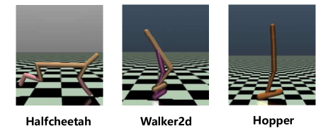
Figure 2: Description of MuJoCo Tasks. The ultimate goal of this task is to utilize algorithms to control the robot’s joints, aiming to make it run as fast and stable as possible.

Experimental Datasets. We employ benchmark tasks commonly studied in OpenAI Gym [35], simulated using the MuJoCo physics engine. The tasks include Halfcheetah-v2, Hopper-v2, and Walker2d-v2, as depicted in Fig. 2. In these MuJoCo environments, the goal is to control the robot’s various joints to achieve faster and more stable locomotion. By applying RL to robot control, the agent observes the state of the MuJoCo environment and controls the robot’s joints based on its learned policy.

For each environment, three types of recorded datasets are considered: Medium, Medium-replay, and Medium-expert. These datasets are based on the work of Fu et al. [36] and the D4RL dataset. The “Medium” dataset is generated by collecting 1 million samples from a policy that undergoes early stopping during online training using SAC [27]. The “Medium-replay” dataset records all samples during the training process, reaching a medium level. The “Medium-expert” dataset is a combination of expert and suboptimal data [36].

Practical algorithm implementation details. Fig. 3 gives the network composition of the algorithm, including environment, discriminator, critic and policy network. Through the discriminator network, the model data sampling probability is calculated for the critic network update; the critic network guides the policy network update; the actions generated on the strategy network generate more model data through the environment model. Table I provides the hyperparameters for network model. The detailed parameter settings for each network update are given below:

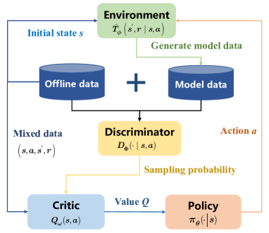
Figure 3: Network composition of the DOMAIN algorithm. The network is composed of four parts: environment, discriminator, critic, and policy.

TABLE I: Base hyperparameter configuration of DOMAIN.

			Parameter	Value
Shared	Parameter		Number of hidden units per layer	256/200
			Number of iterations	1M
			Batch size	256
			Optimizer	Adam
Environment	Model		Model learning rate	1e-4
			Number of hidden layers	4
			Number of model networks $N$	7
			Number of elites $M$	5
			Ratio of model date $f$	0.5
Policy	Learning		Learning rate (policy/critic)	1e-4/3e-4
			Number of hidden layers	2
			Discount factor $\gamma$	0.99
			Soft update parameter $\tau$	5e-3
			Target entropy	-dim(A)
Discriminator	Training		Discriminator learning rate	3e-4
			Number of hidden layers	1
			KL Divergence clipping range	$[10^{-45},10]$
			Dynamics ratio clipping range	$[10^{-45},1]$
			Output layer	2$\times$ Tanh

1) Model Training: The environment model is approximated using a probabilistic network that outputs a Gaussian distribution to obtain the next state and reward. Similar to the approach in [19], we set $N$ as 7 and select the best 5 models. Each model consists of a 4-layer feedforward neural network with 200 hidden units. The model training employs maximum likelihood estimation with a learning rate of 1e-4 and Adam optimizer. The 256 data samples are randomly drawn from the offline dataset $\mathcal{D}_{\text{offline }}$ to calculate the maximum likelihood term.

2) Discriminator Training: Two discriminator networks, $D_{\Phi_{sas}}\left(\cdot\mid s,a,s^{\prime}\right)$ and $D_{\Phi_{sa}}\left(\cdot\mid s,a\right)$, are trained to approximate the probabilities $p\left(\cdot\mid s,a,s^{\prime}\right),p\left(\cdot\mid s,a\right)$. The networks use the prediction “$2\times$ Tanh” activation function to map the output values to the range $[-2,2]$, and then pass the clipped results through a softmax layer to obtain the final probabilities.

3) Policy Optimization: Policy optimization is based on the SAC framework. The critic network $Q_{\omega}$ and the policy network $\pi_{\theta}$ adopt a 2-layer feedforward neural network with 256 hidden units. The learning rates for them are set to 3e-4 and 1e-4 respectively. The ratio of model data in the dataset is $f=0.5$. The entropy regularization coefficient $\alpha$ in Equation (5) is automatically adjusted, with the entropy target set to -dim(A), and the learning rate for the self-tuning network is set to 1e-4.

In practical policy optimization, the obtained adaptive sampling distribution is utilized to select data with high uncertainty and penalize their $Q$-values. Following [13, 21], we sample 10 actions in every high uncertainty state based on the uniform policy Unif(a) and the learned policy $\pi(a\mid s)$, and then estimate the log-sum-exp term in (9) using importance sampling.

Parameter Tuning. The quality of model data is influenced by the environment model $\hat{T}_{\phi}$, the rollout policy $\mu(\cdot\mid s)$, and the rollout horizon $H$. The weight coefficient $\lambda$ of the regularization term significantly affects the stability of agent training. The current learned policy is selected as a rollout policy in all environments. The other parameter tuning results in different environments are as follows (Table III gives the results of D4RL task for different parameters. )

1) Rollout horizon $H$ : Similar to [19, 24], a short-horizon model rollout is performed. The rollout horizon $H$ is chosen from the set $\{1,5\}$. We ues $H=1$ for Walker2d-v2 tasks, and $H=5$ for Hopper-v2 and Halfcheetah-v2 following [21].

2) Weight coefficient $\lambda$ : The parameter $\lambda$ is chosen from the set $\{0.5,5\}$, corresponding to different strengths of regularization. A larger $\lambda$ is needed in narrower data distribution. For medium-replay datasets and halfcheetah-medium datasets, $\lambda$ is chosen as 0.5 , while for the remaining datasets, $\lambda$ is chosen as 5.

V-B Experimental Results

Results on environment model prediction. This section first analyzes and visualizes the accuracy of trained dynamic model prediction before answering the above questions. Fig. 4 gives the prediction results of cumulative error in rollout lengths 1,3,5,7 for different tasks and datasets. In this figure, the predicted errors of four distinct datasets for tasks halfcheetah, hopper and walker2d are arranged from left to right. The prediction error of the trained environmental model exhibits an increasing trend with the increment of steps across all datasets, and the model exhibits the largest prediction error in three walker2d tasks. Therefore, the rollout length is set to 1 in the walker2d task to ensure the stability of the agent.

Results on the D4RL tasks. To answer question 1, this section compares recent model-free algorithms, such as IQL [37], BEAR [9], BRAC [11], and CQL [13], as well as model-based algorithms, including ARMOR [25], MOReL [20], COMBO [21], and RAMBO [24]. The performance of these algorithms is evaluated based on the cumulative return in the robot motion tasks within the MuJoCo environment. A higher score indicates better performance in terms of more stable and faster locomotion control. For comparison, the scores are normalized between 0 (random policy score) and 100 (expert policy score) [36].

Table II presents the normalized scores of different methods. The reported scores are the normalized scores of the learned policies during the last 5 iterations, averaged over 5 random seeds. The results for the model-based methods are obtained from the original papers [20, 21, 24, 25], while the results for the model-free methods are obtained from article [36, 37]. The table shows that the DOMAIN method achieves the best performance in three out of the nine datasets, comparable results in three out of the remaining six settings, and slight poor performance in the three medium settings. Overall, compared to other RL algorithms, the DOMAIN algorithm achieves the best average performance across multiple datasets. Corresponding learning curves are shown in Fig. 5.

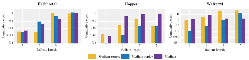
Figure 4: Quantitative analysis of the cumulative model errors. We compare the trained model with the actual MuJoCo environment, with the latter remaining unknown throughout the policy learning process. The initial state is initialized randomly within the MuJoCo environment, and the rollout policy is based on the final learned policy. To facilitate visualization, the logarithmic transformation is employed on the accumulated errors.

TABLE II: Results for the D4RL tasks during the last 5 iterations of training averaged over 5 seeds. $\pm$ captures the standard deviation over seeds. Bold indicates the highest score. Highlighted numbers indicate results within 2% of the most performant algorithm.

Type		Environment	Ours	Model-based baseline				Model-free baseline
			DOMAIN	ARMOR	RAMBO	COMBO	MOReL	CQL	IQL	BRAC-p	BEAR
Medium		Halfcheetah	$72.69\pm 4.66$	$54.2$	$\mathbf{77.6}$	$54.2$	$42.1$	$44.4$	$47.4$	$43.8$	$41.7$
		Hopper	$70.29\pm 8.86$	$\mathbf{101.4}$	$92.8$	$94.9$	$95.4$	$86.6$	$66.3$	$32.7$	$52.1$
		Walker2d	$81.46\pm 0.96$	$\mathbf{90.7}$	$86.9$	$75.5$	$77.8$	$74.5$	$78.3$	$77.5$	$59.1$
Medium	Replay	Halfcheetah	$67.75\pm 3.86$	$50.5$	$\mathbf{68.9}$	$55.1$	$40.2$	$46.2$	$44.2$	$45.4$	$38.6$
		Hopper	$\mathbf{102.68\pm 2.30}$	$97.1$	$96.6$	$73.1$	$93.6$	$48.6$	$94.7$	$0.6$	$33.7$
		Walker2d	$\mathbf{90.36\pm 3.57}$	$85.6$	$85.0$	$56.0$	$49.8$	$32.6$	$73.9$	$73.9$	$19.2$
Medium	Expert	Halfcheetah	$\mathbf{97.74\pm 0.70}$	$93.5$	$93.7$	$90.0$	$53.3$	$62.4$	$86.7$	$44.2$	$53.4$
		Hopper	$109.67\pm 2.18$	$103.4$	$83.3$	$\mathbf{111.1}$	$108.7$	$111.0$	$91.5$	$1.9$	$96.3$
		Walker2d	$110.12\pm 0.12$	$\mathbf{112.2}$	$68.3$	$96.1$	$95.6$	$98.7$	$109.6$	$76.9$	$40.1$
Average Score			$\mathbf{89.20\pm 3.02}$	$87.62$	$83.68$	$78.44$	$72.94$	$67.22$	$76.96$	$35.86$	$48.24$

TABLE III: The results of D4RL task for different parameters. Bolded and highlighted numbers indicate the best performance

Type		Environment	$\lambda=0.5$		$\lambda=5$
			$H=1$	$H=5$	$H=1$	$H=5$
Medium		Halfcheetah	$68.49$	$\mathbf{72.69}$	$51.12$	$49.08$
		Hopper	$0.85$	$69.94$	$64.62$	$\mathbf{70.29}$
		Walker2d	$37.44$	$78.57$	$\mathbf{81.46}$	$-0.10$
Medium	Replay	Halfcheetah	$54.40$	$\mathbf{67.75}$	$50.00$	$46.18$
		Hopper	$84.35$	$\mathbf{102.68}$	$90.53$	$100.6$
		Walker2d	$\mathbf{90.36}$	$85.08$	$87.35$	$52.69$
Medium	Expert	Halfcheetah	$33.24$	$50.31$	$87.82$	$\mathbf{97.74}$
		Hopper	$1.84$	$55.50$	$101.1$	$\mathbf{109.67}$
		Walker2d	$10.72$	$105.78$	$\mathbf{110.12}$	$109.02$

Results on tasks that require generalization. To answer question 2, similar to [21], the halfcheetah-jump environment constructed by [19] is introduced, which requires the agent to solve a task different from the behavioral policy. In the original halfcheetah environment, the objective is to maximize the robot’s running speed, with the reward defined as $r(s,a)=\max\left\{v_{x},3\right\}-0.1\|a\|_{2}^{2}$, where $v_{x}$ denotes the robot’s velocity along the $x$-axis. In the halfcheetah-jump environment, the goal is to make the robot jump as high as possible, and the states of jumping highly are rarely seen in offline states. The rewards in the offline dataset are redefined as $r(s,a)=\max\left\{v_{x},3\right\}-0.1\|a\|_{2}^{2}+15(z-$ init $z)$, where $z$ represents the robot’s position along the $z$-axis and init$z$ denotes the initial position along the $z$-axis.

The datasets used in both cases are collected by training the SAC algorithm for 1 million steps and are similar to the “Medium-expert” dataset in D4RL. Therefore, this dataset serves as the foundation dataset, and the rewards are appropriately modified to obtain the final dataset for training. Table IV presents the normalized scores of different algorithms in the halfcheetah-jump environment. The results for model-based algorithms are sourced from the work of [21], while the results for model-free algorithms are obtained from [19]. It can be observed that the DOMAIN algorithm performs the best, demonstrating stronger generalization capabilities and robustness.

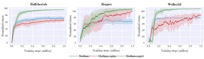
Figure 5: Corresponding learning curves for Table II. Each figure shows the training curve for a specific task under different datasets, where the shaded area represents the standard variance of the return.

TABLE IV: Results for tasks that require generalization during the last 5 iterations of training.

Environment	DOMAIN	COMBO	MoReL	MOPO	MBPO	CQL	SAC	BRAC-p	BEAR
Halfcheetah-jump	$\mathbf{93.65\pm 3.02}$	$45.02$	$28.26$	$34.61$	$26.19$	$8.23$	$-26.64$	$10.87$	$2.39$

TABLE V: The parameter configuration of our designed simple MDP.

Parameter	Designed Dynamic Model							Offline Dataset
	$a$	$[-1,-0.6)$	$[-0.6,-0.2)$	$[-0.2,0.2)$	$[0.2,0.6)$	$[0.6,1]$		Behavioral Policy	Dataset Size
Value	$\mu$	$-a+0.2$	$5(a+0.4)^{2}+0.6$	$-5a^{2}+1$	$10(a-0.4)^{2}+0.4$	$a+0.2$		Random Policy	$1000$
	$\sigma$	$0.06$	$0.04$	$0.02$	$0.04$	$0.06$

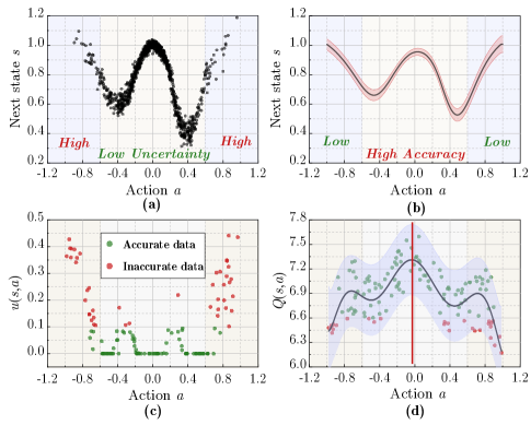
Figure 6: The visualization results of the DOMAIN algorithm on designed MDP. (a) illustrates the distribution of collected offline data. The intermediate color region represents the low uncertainty area, while the region on both sides represents high uncertainty area; (b) presents the prediction results of the trained dynamic model under the initial state ${s=0}$. The red area represents the range of variance predicted by ensemble models; (c) depicts the error distribution of model data. The green color represents precise model data, while the red color represents imprecise model data; (d) illustrates the distribution of $Q$-values of model data. The black curve is the high-order fitting curve of the data. The red line indicates the optimal action, i.e. ${a\approx 0}$.

V-C Visualisation of DOMAIN Performance

Due to the high dimension of states and actions in the D4RL tasks, visualizing the performance is greatly challenging. Therefore, a simple example MDP is defined for illustrative purposes following [24]. For this MDP, both the state space $\mathcal{S}$ and action space $\mathcal{A}\in[-1,1]$ are one-dimensional. The reward is defined as $R(s,a)=s$, where a larger value of state $s$ leads to a higher reward. The dynamic transition model is given by $T(s^{\prime}\mid s,a)=\mathcal{N}(\mu,\sigma)$ with the parameters shown in Table V, indicating that the next state depends on the current action, independent of the initial state. To visualize the DOMAIN exploration in OOD region, we sample actions from $\mathcal{N}(\mu=0,\sigma=0.35)$, which means that the behavioral policy for the offline dataset is random policy.

Fig. 6(a) gives the collected offline data distribution for the above MDP, which illustrates that the actions do not cover all regions. Fig. 6(b) presents the prediction results of trained dynamic model. It can conclude that the dynamic model shows higher prediction accuracy in-distribution region (low uncertain area) but lower prediction accuracy in the OOD region (high uncertain area). Fig. 6(c) displays the model data error after 3000 iterations. It can be observed that the model data within the region exhibits relatively low errors, while the data outside the region shows larger errors. This result is consistent with the prediction results of trained dynamic model. Fig. 6(d) shows the model data $Q$-value curve in state ${s=0}$ after 3000 iterations. We can find that DOMAIN algorithm does not universally underestimate all model data. Instead, it is more prone to underestimating inaccurate model data. Moreover, the value of the optimal action, i.e.,$\arg\max_{a}Q(s,a)$, is approximately equal to zero, which aligns with the selection of the offline dataset. This is because the reward is solely dependent on the state, and the state value is maximized when ${a\approx 0}$ in-distribution region. The consistency between model data and offline data in selecting the optimal actions contributes to enhancing the stability of agent training.

VI Conclusion

This paper proposes a mildly conservative model-based offline RL (DOMAIN) algorithm in this paper. By designing a model data adaptive sampling distribution, this algorithm can dynamically adjust the model data penalties, increasing the penalty for model data with larger errors while reducing the penalty for accurate model data, thereby reducing its conservatism. Moreover, DOMAIN avoids unreliable estimation of model uncertainty. Theoretical analysis demonstrates that DOMAIN can guarantee safe policy improvements and $Q$-values learned by DOMAIN outside the region are lower bounds of the true $Q$-values. Experimental results on the D4RL benchmark show that DOMAIN outperforms previous RL algorithms on most datasets and achieves the best generalization performance in tasks that require adaptation to unseen behaviors. However, since incorporating conservatism during the training process constrains the improvement of agent performance, future efforts can focus on optimizing the environment model itself to further enhance the overall performance.

Appendix A Proof of Relevant Theorems

A-A Proof of Theorem 1

Before proof, we provide a notation clarification. Let $\mathcal{T}^{\pi}$ denote the ideal Bellman operator, and $\hat{\mathcal{T}}^{\pi}$ represents the actual Bellman operator. $\mathcal{M}$ refers to the true MDP, $\hat{\mathcal{M}}$ represents the learned MDP model, and $\bar{\mathcal{M}}$ denotes the empirical MDP, where “empirical” refers to operations based on samples. $\mathcal{T}_{\mathcal{M}}^{\pi},T_{\mathcal{M}}$, and $r_{\mathcal{M}}$ denote the Bellman operator, state transition, and reward under the true $\mathrm{MDP}\mathcal{M}$, respectively. $\mathcal{T}_{\hat{\mathcal{M}}}^{\pi},T_{\hat{\mathcal{M}}}$, and $r_{\hat{\mathcal{M}}}$ represent the corresponding operators under the learned MDP $\hat{\mathcal{M}}$, while $\mathcal{T}_{\bar{\mathcal{M}}}^{\pi},T_{\bar{\mathcal{M}}}$ and $r_{\bar{\mathcal{M}}}$ denote the operators under the empirical MDP $\bar{\mathcal{M}}$. It should be noted that $\mathcal{T}^{\pi}=\mathcal{T}_{\mathcal{M}}^{\pi}$ and $\hat{\mathcal{T}}^{\pi}=(1-f)\mathcal{T}_{\hat{\mathcal{M}}}^{\pi}+f\mathcal{T}_{\hat{\mathcal{M}}}^{\pi}$. Considering the sampling error of the empirical MDP, we make the following assumptions, following prior works [13, 21, 31, 34] :

Assumption 1

For $\forall s,a\in\mathcal{D}$, the following inequality holds with a probability greater than $1-\delta$, where $\delta\in(0,1)$:

$$\left|r_{\mathcal{M}}(s,a)-r_{\bar{\mathcal{M}}}(s,a)\right|<\frac{C_{r,\delta}}{\sqrt{|\mathcal{D}(s,a)|}}$$ (18)

$$\left|T_{\mathcal{M}}\left(s^{\prime}\mid s,a\right)-T_{\bar{\mathcal{M}}}\left(s^{\prime}\mid s,a\right)\right|_{1}<\frac{C_{T,\delta}}{\sqrt{|\mathcal{D}(s,a)|}}$$

where $|\mathcal{D}(s,a)|$ represents the cardinality (number of occurrences) of a specific state-action pair $(s,a)$ in the dataset $\mathcal{D}$. For $(s,a)\notin\mathcal{D}$, we assume $|\mathcal{D}(s,a)|$ to be less than 1. The reward is bounded within a certain range, given by $\left|r_{\mathcal{M}}(s,a)\right|<R_{\max}$.

Lemma 1

For any policy $\pi$, the disparity between the actual Bellman operator $\mathcal{T}_{\mathcal{M}}^{\pi}$ and the Bellman operators $\mathcal{T}_{\bar{\mathcal{M}}}^{\pi}$ under the empirical MDP, as well as the disparity between the actual Bellman operator $\mathcal{T}_{\mathcal{M}}^{\pi}$ and the Bellman operators $\mathcal{T}_{\hat{\mathcal{M}}}^{\pi}$ under the learned MDP can be expressed as, respectively:

$$\left|\left(\mathcal{T}_{\mathcal{M}}^{\pi}\hat{Q}^{k}\right)-\left(\mathcal{T}_{\bar{\mathcal{M}}}^{\pi}\hat{Q}^{k}\right)\right|<\frac{C_{r,T,\delta}R_{\max}}{(1-\gamma)\sqrt{|\mathcal{D}(s,a)|}}$$ (19)

$$\left|\left(\mathcal{T}_{\mathcal{M}}^{\pi}\hat{Q}^{k}\right)-\left(\mathcal{T}_{\hat{\mathcal{M}}}^{\pi}\hat{Q}^{k}\right)\right|<\varepsilon_{r}+D\left(T_{\mathcal{M}},T_{\hat{\mathcal{M}}}\right)\frac{2\gamma R_{\max}}{1-\gamma}$$

Proof. The difference between the Bellman operator $\mathcal{T}_{\hat{\mathcal{M}}}^{\pi}$ under the empirical MDP and the actual Bellman operator $\mathcal{T}_{\mathcal{M}}^{\pi}$ is given by:

$$\left|\left(\mathcal{T}_{\mathcal{M}}^{\pi}\hat{Q}^{k}\right)-\left(\mathcal{T}_{\bar{\mathcal{M}}}^{\pi}\hat{Q}^{k}\right)\right|$$ (20)

$$\leq \left|r_{\mathcal{M}}(s,a)-r_{\bar{\mathcal{M}}}(s,a)\right|+\gamma\left|\sum_{s^{\prime}}(T_{\mathcal{M}}\left(s^{\prime}\mid s,a\right)\right.$$

$$\left.-T_{\bar{\mathcal{M}}}\left(s^{\prime}\mid s,a\right))\mathbb{E}_{a^{\prime}\sim\pi}\left[\hat{Q}^{k}\left(s^{\prime},a^{\prime}\right)\right]\right|$$

$$\leq \frac{(1-\gamma)C_{r,\delta}+\gamma C_{T,\delta}2R_{\max}}{(1-\gamma)\sqrt{|\mathcal{D}(s,a)|}}=\frac{C_{r,T,\delta}R_{\max}}{(1-\gamma)\sqrt{|\mathcal{D}(s,a)|}}$$

Here, $C_{r,T,\delta}$ is a function representing a combination of $C_{r,\delta}$ and $C_{T,\delta}$. Similarly, the difference between the Bellman operator $\mathcal{T}_{\hat{\mathcal{M}}}^{\pi}$ under the learned MDP and the actual Bellman operator $\mathcal{T}_{\mathcal{M}}^{\pi}$ can be derived as:

$$\left|\left(\mathcal{T}_{\mathcal{M}}^{\pi}\hat{Q}^{k}\right)-\left(\mathcal{T}_{\hat{\mathcal{M}}}^{\pi}\hat{Q}^{k}\right)\right|$$ (21)

$$\leq \left|r_{\mathcal{M}}(s,a)-r_{\hat{\mathcal{M}}}(s,a)\right|+\gamma\left|\sum_{s^{\prime}}(T_{\mathcal{M}}\left(s^{\prime}\mid s,a\right)\right.$$

$$\left.-T_{\hat{\mathcal{M}}}\left(s^{\prime}\mid s,a\right))\mathbb{E}_{a^{\prime}\sim\pi}\left[\hat{Q}^{k}\left(s^{\prime},a^{\prime}\right)\right]\right|$$

$$\leq \left|r_{\mathcal{M}}(s,a)-r_{\hat{\mathcal{M}}}(s,a)\right|+D\left(T_{\mathcal{M}},T_{\hat{\mathcal{M}}}\right)\frac{2\gamma R_{\max}}{1-\gamma}$$

where $\varepsilon_{r}(s,a)$ represents the error between the learned reward and the actual reward, and $D\left(T_{\mathcal{M}},T_{\hat{\mathcal{M}}}\right)$ denotes the discrepancy between the transitions of the learned model and the true model. Lemma 1 is thus proven.

The proof derivation of Theorem 1 is presented below. First, we introduce the following notation: Let $\mathcal{T}^{\pi}Q=r+\gamma P^{\pi}Q$, where $P^{\pi}Q(s,a)=\mathbb{E}_{s^{\prime}\sim T(\cdot\mid s,a),a^{\prime}\sim\pi(\cdot\mid s^{\prime})}[Q^{\pi}(s^{\prime},a^{\prime})]$. Based on Equation (14) and the Lemma 1, it can obtain:

$$\hat{Q}^{k+1}=(1-f)\mathcal{T}_{\bar{\mathcal{M}}}^{{\pi}}\hat{Q}^{k}+f\hat{\mathcal{T}}_{\hat{\mathcal{M}}}^{\pi}\hat{Q}^{k}-\lambda\eta(s,a)$$ (22)

$$\leq \mathcal{T}_{\mathcal{M}}^{\pi}\hat{Q}^{k}+(1-f)\underbrace{\frac{C_{r,T,\delta}R_{\max}}{(1-\gamma)\sqrt{|\mathcal{D}(s,a)|}}}_{:=\Delta_{1}(s,a)}-\lambda\eta(s,a)$$

$$+f(\underbrace{\left|r_{\mathcal{M}}-r_{\hat{\mathcal{M}}}\right|+D\left(T_{\mathcal{M}},T_{\hat{\mathcal{M}}}\right)\frac{2\gamma R_{\max}}{1-\gamma}}_{:=\Delta_{2}(s,a)})$$

$$= \mathcal{T}^{\pi}\hat{Q}^{k}+\underbrace{(1-f)\Delta_{1}(s,a)+f\Delta_{2}(s,a)-\lambda\eta(s,a)}_{:=\Delta(s,a)})$$

By applying the fixed-point theorem, the above equation leads to:

$$\hat{Q}^{\pi} \leq\mathcal{T}^{\pi}\hat{Q}^{\pi}+\Delta=r+\gamma P^{\pi}\hat{Q}^{\pi}+\Delta$$ (23)

$$\Rightarrow\hat{Q}^{\pi} \leq\left(I-\gamma P^{\pi}\right)^{-1}(r+\Delta)$$

$$=\left(I-\gamma P^{\pi}\right)^{-1}r+\left(I-\gamma P^{\pi}\right)^{-1}\Delta$$

Since $\mathcal{T}^{\pi}Q:=Q=r+\gamma P^{\pi}Q\Rightarrow Q=\left(I-\gamma P^{\pi}\right)^{-1}r$, the above equation can be further derived as:

$$\hat{Q}^{\pi}(s,a)\leq Q^{\pi}(s,a)+\left(I-\gamma P^{\pi}\right)^{-1}\Delta(s,a)$$ (24)

Based on the value function $V^{\pi}(s)=\mathbb{E}_{a\sim\pi(a\mid s)}\left[Q^{\pi}(s,a)\right]$, it can derive:

$$\hat{V}^{\pi}(s)\leq V^{\pi}(s)+\left(I-\gamma P^{\pi}\right)^{-1}\mathbb{E}_{a\sim\pi(a\mid s)}[\Delta(s,a)]$$ (25)

To ensure the lower bound, $\lambda$ can be chosen to avoid overestimation. Moreover, since the expression $\left(I-\gamma P^{\pi}\right)^{-1}$ is positive semi-definite, as long as $\mathbb{E}_{a\sim\pi(a\mid s)}[\Delta(s,a)]<0$, the choice of $\lambda$ can be controlled by the following condition:

$$\lambda\cdot\min_{s}\mathbb{E}_{a\sim\pi(a\mid s)}[\eta(s,a)]$$ (26)

$$\geq \max_{s}\mathbb{E}_{a\sim\pi(a\mid s)}\left[(1-f)\Delta_{1}(s,a)+f\Delta_{2}(s,a)\right]$$

Since $\Delta_{1}(s,a)>0,\Delta_{2}(s,a)>0,\lambda>0$, in order for Equation (26) to satisfy the condition, it is a prerequisite that the term $\min\mathbb{E}_{a\sim\pi(a\mid s)}[\eta(s,a)]>0$ holds, leading to:

$$\mathbb{E}_{a\sim\pi(a\mid s)}[\eta(s,a)]$$ (27)

$$= \mathbb{E}_{a\sim\pi(a\mid s)}\left[\frac{\omega(s,a)-d(s,a)}{(1-f)d^{\pi_{b}}(s,a)+fd_{\hat{\mathcal{M}}}^{\pi}(s,a)}\right]$$

$$= \sum_{a}\frac{\omega(s,a)}{(1-f)d^{\pi_{b}}(s)\frac{\pi_{b}(a\mid s)}{\pi(a\mid s)}+fd_{\mathcal{\hat{\mathcal{M}}}}^{\pi}(s)}$$

$$-\sum_{a}\frac{d(s,a)}{(1-f)d^{\pi_{b}}(s)\frac{\pi_{b}(a\mid s)}{\pi(a\mid s)}+fd_{\hat{\mathcal{M}}}^{\pi}(s)}$$

$$\geq \frac{\sum_{a}\omega(s,a)}{(1-f)d^{\pi_{b}}(s)\max_{a}\left\{\frac{\pi_{b}(a\mid s)}{\pi(a\mid s)}\right\}+fd_{\hat{\mathcal{M}}}^{\pi}(s)}$$

$$-\frac{\sum_{a}d(s,a)}{(1-f)d^{\pi_{b}}(s)\min_{a}\left\{\frac{\pi_{b}(a\mid s)}{\pi(a\mid s)}\right\}+fd_{\hat{\mathcal{\mathcal{M}}}}^{\pi}(s)}$$

Consequently, the condition for $\min\mathbb{E}_{a\sim\pi(a\mid s)}[\eta(s,a)]>0$ to hold is derived as follows:

$$\sum_{a}\omega(s,a)$$ (28)

$$> \frac{(1-f)d^{\pi_{b}}(s)\max_{a}\left\{\frac{\pi_{b}(a\mid s)}{\pi(a\mid s)}\right\}+fd_{\hat{\mathcal{M}}}^{\pi}(s)}{(1-f)d^{\pi_{b}}(s)\min_{a}\left\{\frac{\pi_{b}(a\mid s)}{\pi(a\mid s)}\right\}+fd_{\hat{\mathcal{M}}}^{\pi}(s)}\sum_{a}d(s,a)$$

$$= \xi(s)\sum_{a}d(s,a)$$

Substituting Equation (28) into (26), it can further derive:

$$\lambda\cdot\min_{s}\frac{(\xi(s)-1)\sum_{a}d(s,a)}{(1-f)d^{\pi_{b}}(s)\max_{a}\left\{\frac{\pi_{b}(a\mid s)}{\pi(a\mid s)}\right\}+fd_{\hat{\mathcal{M}}}^{\pi}(s)}$$ (29)

$$\geq (1-f)\frac{C_{r,T,\delta}R_{\max}}{(1-\gamma)\min_{s,a}\{\sqrt{|\mathcal{D}(s,a)|}\}}$$

$$+f\left[\max_{s,a}\left\{\left|r_{\mathcal{M}}-r_{\hat{\mathcal{M}}}\right|\right\}+\frac{2\gamma R_{\max}}{1-\gamma}\max_{s,a}\left\{D\left(T_{\hat{\mathcal{M}}},T_{\mathcal{M}}\right)\right\}\right]$$

$$\Rightarrow \lambda\geq\frac{(1-f)\frac{C_{r,T,\delta}R_{\max}}{(1-\gamma)\min_{s,a}\{\sqrt{|\mathcal{D}|}\}}}{\min_{s}\left\{\frac{(\xi(s)-1)\sum_{a}d(s,a)}{\left[(1-f)d^{\pi_{b}}(s)\max_{a}\left\{\frac{\pi_{b}(a\mid s)}{\pi(a\mid s)}\right\}+fd_{\hat{\mathcal{M}}}^{\pi}(s)\right]}\right\}}$$

$$+\frac{f[\max\limits_{s,a}\left\{\left|r_{\mathcal{M}}-r_{\mathcal{M}}\right|\right\}+\frac{2\gamma R_{\max}}{1-\gamma}\max\limits_{s,a}\left\{D_{TV}\left(T_{\mathcal{M}},T_{\hat{\mathcal{M}}}\right)\right\}]}{\min_{s}\left\{\frac{(\xi(s)-1)\sum_{a}d(s,a)}{\left[(1-f)d^{\pi_{b}}(s)\max_{a}\left\{\frac{\pi_{b}(a\mid s)}{\pi(a\mid s)}\right\}+fd_{\hat{\mathcal{M}}}^{\pi}(s)\right]}\right\}}$$

Thus, Theorem 1 is proved.

A-B Proof of Theorem 2

Yu et al. [21] give expression: $\hat{Q}^{k+1}(s,a)=(\hat{\mathcal{T}}^{\pi}\hat{Q}^{k})(s,a)-\lambda[\frac{\rho(s,a)-d(s,a)}{(1-f)d(s,a)+f\rho(s,a)}]$. Assuming DOMAIN and COMBO methods have the same sampling and model errors, we have:

$$\kappa_{1}-\kappa_{2}$$ (30)

$$= \mathbb{E}_{s\sim d(s),a\sim\pi(a\mid s)}\left[\hat{Q}_{1}^{\pi}(s,a)-\hat{Q}_{2}^{\pi}(s,a)\right]$$

$$= \mathbb{E}_{s\sim d(s)}\left[\sum_{a}\frac{\pi(a\mid s)\left[\rho(s,a)-\omega(s,a)\right]}{(1-f)d^{\pi_{b}}(s)\pi_{b}(a\mid s)+fd_{\hat{\mathcal{M}}}^{\pi}(s)\pi(a\mid s)}\right]$$

$$\geq \mathbb{E}_{s\sim d(s)}\left[\frac{\sum_{a}(\rho(s,a)-\omega(s,a))}{(1-f)d^{\pi_{b}}(s)\max_{a}\left\{\frac{\pi_{b}(a\mid s)}{\pi(a\mid s})\right\}+fd_{\hat{\mathcal{M}}}^{\pi}(s)}\right]$$

$$\geq \underbrace{\frac{\mathbb{E}_{s\sim d(s)}\left[d_{\hat{\mathcal{M}}}^{\pi}(s)\right]-\mathbb{E}_{s\sim d(s),a\sim\pi(a\mid s)}[\omega(s,a)]}{\max_{s}\left\{(1-f)d^{\pi_{b}}(s)\max_{a}\left\{\frac{\pi_{b}(a\mid s)}{\pi(a\mid s)}\right\}+fd_{\hat{\mathcal{M}}}^{\pi}(s)\right\}}}_{>0}$$

where $d(s)$ represents the state distribution of the dataset, which can be an offline dataset, a model dataset, or the overall dataset. When $\mathbb{E}_{s\sim d(s)}[d_{\hat{\mathcal{M}}}^{\pi}(s)]\geq\mathbb{E}_{s\sim d(s),a\sim\pi(a\mid s)}[\omega(s,a)]$, the average value function of the DOMAIN method on the dataset is greater than that of COMBO. In other words, under the aforementioned condition, DOMAIN is less conservative than COMBO. Thus, Theorem 2 is proved.

A-C Proof of Theorem 3

RL aims to maximize the cumulative return, denoted as $\pi^{*}=\max_{\pi}J(\mathcal{M},\pi):=\frac{1}{1-\gamma}\mathbb{E}_{(s,a)\sim d_{\mathcal{M}}^{\pi}(s,a)}[r(s,a)]$. Before proving Theorem 3, we present two lemmas.

Lemma 2

For any $\mathcal{M}$ and the experience $\bar{\mathcal{M}}$ generated by sampling according to the behavioral policy $\pi_{b}$, the performance of both $\mathcal{M}$ and $\bar{\mathcal{M}}$ under policy $\pi$ satisfies:

$$|J(\mathcal{M},\pi)-J(\bar{\mathcal{M}},\pi)|$$ (31)

$$\leq \frac{1}{1-\gamma}\mathbb{E}_{(s,a)\sim d_{\bar{\mathcal{M}}}^{\pi}(s,a)}\left[\frac{C_{r,\delta}+R_{\max}C_{T,\delta}}{\sqrt{|\mathcal{D}(s,a)|}}\right]$$

Proof. The proof follows a similar approach to Kumar et al. [13]. Firstly, we employ the triangle inequality to separate the reward return and the dynamic properties:

$$|J(\mathcal{M},\pi)-J(\bar{\mathcal{M}},\pi)|$$ (32)

$$= \frac{1}{1-\gamma}\left|\sum_{s,a}d_{\bar{\mathcal{M}}}^{\pi}(s)\pi(a\mid s)r_{\bar{\mathcal{M}}}-d_{\mathcal{M}}^{\pi}(s)\pi(a\mid s)r_{\mathcal{M}}\right|$$

$$\leq \frac{1}{1-\gamma}\left|\sum_{s,a}d_{\bar{\mathcal{M}}}^{\pi}(s)\pi(a\mid s)\left[r_{\bar{\mathcal{M}}}(s,a)-r_{\mathcal{M}}(s,a)\right]\right|$$

$$+\frac{1}{1-\gamma}\left|\sum_{s,a}\left(d_{\bar{\mathcal{M}}}^{\pi}(s)-d_{\mathcal{M}}^{\pi}(s)\right)\pi(a\mid s)r_{\mathcal{M}}(s,a)\right|$$

Based on Assumption 1, it can express the first term above as:

$$\left|\sum_{s,a}d_{\bar{\mathcal{M}}}^{\pi}(s)\pi(a\mid s)\left[r_{\bar{\mathcal{M}}}-r_{\mathcal{M}}\right]\right|\leq\mathbb{E}_{(s,a)\sim d_{\bar{\mathcal{M}}}^{\pi}}\left[\frac{C_{r,\delta}}{\sqrt{|\mathcal{D}(s,a)|}}\right]$$ (33)

Following the proof of Kumar et al. [13] on the upper bound of $\left|d_{\bar{\mathcal{M}}}^{\pi}(s)-d_{\mathcal{\mathcal{M}}}^{\pi}(s)\right|$, we have:

$$\left|d_{\bar{\mathcal{M}}}^{\pi}(s)-d_{\mathcal{M}}^{\pi}(s)\right|$$ (34)

$$\leq \sum_{s,s^{\prime}}\left|\sum_{a}\left(T_{\bar{\mathcal{M}}}\left(s^{\prime}\mid s,a\right)-T_{\mathcal{M}}\left(s^{\prime}\mid s,a\right)\right)\pi(a\mid s)\right|d_{\bar{\mathcal{M}}}^{\pi}(s)$$

From Assumption 1, it can deduce that $\left|d_{\bar{\mathcal{M}}}^{\pi}(s)-d_{\mathcal{M}}^{\pi}(s)\right|\leq\mathbb{E}_{(s,a)\sim d_{\mathcal{M}}^{\pi}(s,a)}\left[\frac{C_{T,\delta}}{\sqrt{|\mathcal{D}(s,a)|}}\right]$, resulting in an upper bound for the second term in Equation (32):

$$\left|\sum_{s,a}\left(d_{\bar{\mathcal{M}}}^{\pi}(s)-d_{\mathcal{M}}^{\pi}(s)\right)\pi(a\mid s)r_{\mathcal{M}}(s,a)\right|$$ (35)

$$\leq \mathbb{E}_{(s,a)\sim d_{\mathcal{\bar{\mathcal{M}}}}^{\pi}(s,a)}\left[\frac{R_{\max}C_{T,\delta}}{\sqrt{|\mathcal{D}(s,a)|}}\right]$$

Further derivation leads to:

$$|J(\mathcal{M},\pi)-J(\bar{\mathcal{M}},\pi)|$$ (36)

$$\leq \frac{1}{1-\gamma}\mathbb{E}_{(s,a)\sim d_{\bar{\mathcal{M}}}^{\pi}(s,a)}\left[\frac{C_{r,\delta}+R_{\max}C_{T,\delta}}{\sqrt{|\mathcal{D}(s,a)|}}\right]$$

Lemma 2 is thus proven.

Lemma 3

For any $\mathcal{M}$ and an MDP $\hat{\mathcal{M}}$ learned on the offline dataset, their performance on policy $\pi$ satisfies:

$$|J(\mathcal{M},\pi)-J(\hat{\mathcal{M}},\pi)|$$ (37)

$$\leq \frac{1}{1-\gamma}\mathbb{E}_{(s,a)\sim d_{\hat{\mathcal{M}}}^{\pi}(s,a)}\left[\varepsilon_{r}(s,a)+R_{\max}D(s,a)\right]$$

Proof. The proof follows a similar process as in Lemma 2. First, it can deduce:

$$|J(\mathcal{M},\pi)-J(\hat{\mathcal{M}},\pi)|$$ (38)

$$\leq \frac{1}{1-\gamma}\left|\sum_{s,a}d_{\hat{\mathcal{M}}}^{\pi}(s)\pi(a\mid s)\left[r_{\hat{\mathcal{M}}}(s,a)-r_{\mathcal{M}}(s,a)\right]\right|$$

$$+\frac{1}{1-\gamma}\left|\sum_{s,a}\left(d_{\hat{\mathcal{M}}}^{\pi}(s)-d_{\mathcal{M}}^{\pi}(s)\right)\pi(a\mid s)r_{\mathcal{M}}(s,a)\right|$$

Let $\left|r_{\hat{\mathcal{M}}}(s,a)-r_{\mathcal{M}}(s,a)\right|=\varepsilon_{r}(s,a)$ denote the reward prediction error, and $\left|\left(T_{\bar{\mathcal{M}}}\left(s^{\prime}\mid s,a\right)-T_{\mathcal{M}}\left(s^{\prime}\mid s,a\right)\right)\right|_{1}=D(s,a)$ denote the state transition prediction error. Consequently, it can obtain:

$$|J(\mathcal{M},\pi)-J(\hat{\mathcal{M}},\pi)|$$ (39)

$$\leq \frac{1}{1-\gamma}\mathbb{E}_{(s,a)\sim d_{\hat{\mathcal{M}}}^{\pi}(s,a)}\left[\varepsilon_{r}(s,a)+R_{\max}D(s,a)\right]$$

Lemma 3 is thus proven. Let $\hat{Q}^{\pi}(s,a)$ denote the fixed point of Equation (14). The policy update for the DOMAIN method is expressed as follows:

$$\pi^{*}=\max_{\pi}\left[J\left(\mathcal{M}_{f},\pi\right)-\frac{\lambda}{1-\gamma}\mathbb{E}_{(s,a)\sim d_{\mathcal{M}_{f}}^{\pi}}[\eta(s,a)]\right]$$ (40)

where $J\left(\mathcal{M}_{f},\pi\right)=(1-f)J(\bar{\mathcal{M}},\pi)+fJ(\hat{\mathcal{M}},\pi)$, $\mathcal{M}_{f}:=(1-f)\bar{\mathcal{M}}+f\hat{\mathcal{M}}$, and $\eta(s,a)=(\omega(s,a)-d(s,a))/d_{\beta}(s,a)$. Since $\pi^{*}$ represents the optimal value in Equation (40), and let $\varpi(\pi,f)=\mathbb{E}_{(s,a)\sim d_{\mathcal{M}_{f}}^{\pi}}[\eta(s,a)]$, we have:

$$J\left(\mathcal{M}_{f},\pi^{*}\right)-\frac{\lambda\varpi\left(\pi^{*},f\right)}{1-\gamma}\geq J\left(\mathcal{M}_{f},\pi_{b}\right)-\frac{\lambda\varpi\left(\pi_{b},f\right)}{1-\gamma}$$ (41)

In order to compare the performance of the learned policy $\pi^{*}$ and the behavioral policy $\pi_{b}$ on the actual MDP, Theorem 3 employs the triangle inequality to deduce:

$$\left|J\left(\mathcal{M}_{f},\pi\right)-J(\mathcal{M},\pi)\right|$$ (42)

$$= |(1-f)J(\bar{\mathcal{M}},\pi)+fJ(\hat{\mathcal{M}},\pi)-J(\mathcal{M},\pi)|$$

$$\leq (1-f)|J(\mathcal{M},\pi)-J(\bar{\mathcal{M}},\pi)|+f|J(\mathcal{M},\pi)-J(\hat{\mathcal{M}},\pi)|$$

By utilizing Lemma 2 and 3, it can infer:

$$\left|J\left(\mathcal{M}_{f},\pi\right)-J(\mathcal{M},\pi)\right|$$ (43)

$$\leq (1-f)|J(\mathcal{M},\pi)-J(\bar{\mathcal{M}},\pi)|+f|J(\mathcal{M},\pi)-J(\hat{\mathcal{M}},\pi)|$$

$$\leq \frac{1-f}{1-\gamma}\mathbb{E}_{(s,a)\sim d_{\mathcal{M}}^{\pi}(s,a)}\left[\frac{C_{r,\delta}+R_{\max}C_{T,\delta}}{\sqrt{|\mathcal{D}(s,a)|}}\right]$$

$$+\frac{f}{1-\gamma}\mathbb{E}_{(s,a)\sim d_{\mathcal{M}}^{\pi}(s,a)}\left[\varepsilon_{r}(s,a)+R_{\max}D(s,a)\right]$$

Substituting Equation (43) into (41), it can further derive:

$$J\left(\mathcal{M},\pi^{*}\right)-J\left(\mathcal{M},\pi_{b}\right)$$ (44)

$$\geq \frac{\lambda}{1-\gamma}\left[\varpi\left(\pi^{*},f\right)-\varpi\left(\pi_{b},f\right)\right]$$

$$-\frac{1-f}{1-\gamma}\left\{\mathbb{E}_{(s,a)\sim d_{\mathcal{M}}^{*}}\left[\frac{C_{r,\delta}+R_{\max}C_{T,\delta}}{\sqrt{|\mathcal{D}(s,a)|}}\right]\right.$$

$$\left.+\mathbb{E}_{(s,a)\sim d_{\mathcal{M}}^{\pi_{b}}}\left[\frac{C_{r,\delta}+R_{\max}C_{T,\delta}}{\sqrt{|\mathcal{D}(s,a)|}}\right]\right\}$$

$$-\frac{f}{1-\gamma}\left\{\mathbb{E}_{(s,a)\sim d_{\mathcal{M}}^{\pi^{*}}}\left[\varepsilon_{r}(s,a)+R_{\max}D(s,a)\right]\right.$$

$$\left.+\mathbb{E}_{(s,a)\sim d_{\mathcal{M}}^{\pi_{b}}}\left[\varepsilon_{r}(s,a)+R_{\max}D(s,a)\right]\right\}$$

The behavioral policy $\pi_{b}$ is obtained from the offline dataset $\mathcal{D}_{\text{offline }}$, resulting in a larger $\sqrt{|\mathcal{D}(s,a)|}$ under the distribution $d_{\bar{\mathcal{M}}}^{\pi_{b}}$, indicating smaller sampling errors. Additionally, since the environment model is trained using $\mathcal{D}_{\text{offline }}$, the model error is smaller under the distribution $d_{\hat{\mathcal{M}}}^{\pi_{b}}$. Therefore, Equation (44) can be further simplified as:

$$J\left(\mathcal{M},\pi^{*}\right)-J\left(\mathcal{M},\pi_{b}\right)$$ (45)

$$\geq \frac{\lambda}{1-\gamma}\left[\varpi\left(\pi^{*},f\right)-\varpi\left(\pi_{b},f\right)\right]$$

$$-2\frac{1-f}{1-\gamma}\mathbb{E}_{(s,a)\sim d\pi_{\mathcal{M}}^{*}}\left[\frac{C_{r,\delta}+R_{\max}C_{T,\delta}}{\sqrt{|\mathcal{D}(s,a)|}}\right]$$

$$-2\frac{f}{1-\gamma}\mathbb{E}_{(s,a)\sim d_{\mathcal{M}}^{\pi^{*}}}\left[\varepsilon_{r}(s,a)+R_{\max}D(s,a)\right]$$

Theorem 3 is proved.

References

• [1] D. Kalashnikov et al., “Scalable deep reinforcement learning for vision-based robotic manipulation,” in Conf. Robot Learn., 2018, pp. 651-673.
• [2] Y. Wen, J. Si, A. Brandt, X. Gao, and H. H. Huang, “Online reinforcement learning control for the personalization of a robotic knee prosthesis,” IEEE Trans. Cybern., vol. 50, no. 6, pp. 2346-2356, 2019.
• [3] F. Yu et al., “Bdd100k: A diverse driving dataset for heterogeneous multitask learning,” in Proc. IEEE Conf. Comput. Vis. Pattern Recognit., 2020, pp. 2636-2645.
• [4] A. Swaminathan and T. Joachims, “Batch learning from logged bandit feedback through counterfactual risk minimization,” J. Mach. Learn. Res., vol. 16, no. 1, pp. 1731-1755, 2015.
• [5] H. Mao, M. Schwarzkopf, S. B. Venkatakrishnan, Z. Meng, and M. Alizadeh, “Learning scheduling algorithms for data processing clusters,” in Pro. ACM Special Interest Group Data Commun., 2019, pp. 270-288.
• [6] T. T. Nguyen, N. D. Nguyen, and S. Nahavandi, “Deep Reinforcement Learning for Multiagent Systems: A Review of Challenges, Solutions, and Applications,” IEEE Trans. Cybern., vol. 50, no. 9, pp. 3826-3839, 2020.
• [7] J. Chen, and W. Xu, “Policy Gradient From Demonstration and Curiosity,” IEEE Trans. Cybern., vol. 53, no. 8, pp. 4923-4933, 2023.
• [8] S. Levine, A. Kumar, G. Tucker, and J. Fu, “Offline reinforcement learning: Tutorial, review, and perspectives on open problems,” 2020. [Online]. Available: arXiv:2005.01643.
• [9] A. Kumar, J. Fu, M. Soh, G. Tucker, and S. Levine, “Stabilizing off-policy q-learning via bootstrapping error reduction,” in Proc. Adv. Neural Inf. Process. Syst., 2019, pp. 11784-11794.
• [10] S. Fujimoto, D. Meger, and D. Precup, “Off-policy deep reinforcement learning without exploration,” in Int. Conf. Mach. Learn., 2019, pp. 2052-2062.
• [11] Y. Wu, G. Tucker, and O. Nachum, “Behavior regularized offline reinforcement learning,” 2019. [Online]. Available: arXiv:1911.11361.
• [12] C. Zhang, S. Kuppannagari, and P. Viktor, “Brac+: Improved behavior regularized actor critic for offline reinforcement learning,” in Asian Conf. Mach. Learn., 2021, pp. 204-219.
• [13] A. Kumar, A. Zhou, G. Tucker, and S. Levine, “Conservative q-learning for offline reinforcement learning,” in Proc. Adv. Neural Inf. Process. Syst., 2020, pp. 1179-1191.
• [14] S. Fujimoto and S. S. Gu, “A minimalist approach to offline reinforcement learning,” in Proc. Adv. Neural Inf. Process. Syst., 2021, pp. 20132-20145.
• [15] J. Lyu, X. Ma, X. Li, and Z. Lu, “Mildly conservative Q-learning for offline reinforcement learning,” in Proc. Adv. Neural Inf. Process. Syst., 2022, pp. 1711-1724.
• [16] L. Kaiser et al., “Model Based Reinforcement Learning for Atari,” in Int. Conf. Learn. Represent., 2019.
• [17] F.-M. Luo, T. Xu, H. Lai, X.-H. Chen, W. Zhang, and Y. Yu, “A survey on model-based reinforcement learning,” 2022. [Online]. Available: arXiv:2206.09328.
• [18] W.-C. Jiang, V. Narayanan, and J.-S. Li, “Model learning and knowledge sharing for cooperative multiagent systems in stochastic environment,” IEEE Trans. Cybern., vol. 51, no. 12, pp. 5717-5727, 2020.
• [19] T. Yu et al., “Mopo: Model-based offline policy optimization,” in Proc. Adv. Neural Inf. Process. Syst., 2020, pp. 14129-14142.
• [20] R. Kidambi, A. Rajeswaran, P. Netrapalli, and T. Joachims, "Morel: Model-based offline reinforcement learning," in Proc. Adv. Neural Inf. Process. Syst., 2020, pp. 21810-21823.
• [21] T. Yu, A. Kumar, R. Rafailov, A. Rajeswaran, S. Levine, and C. Finn, “Combo: Conservative offline model-based policy optimization,” in Proc. Adv. Neural Inf. Process. Syst., 2021, pp. 28954-28967.
• [22] O. Kroemer, S. Niekum, and G. Konidaris, “A review of robot learning for manipulation: Challenges, representations, and algorithms,” J. Mach. Learn. Res., vol. 22, no. 1, pp. 1395-1476, 2021.
• [23] M. Janner, J. Fu, M. Zhang, and S. Levine, “When to trust your model: Model-based policy optimization,” in Proc. Adv. Neural Inf. Process. Syst., 2019, pp. 12519-12530.
• [24] M. Rigter, B. Lacerda, and N. Hawes, “Rambo-rl: Robust adversarial model-based offline reinforcement learning,” in Proc. Adv. Neural Inf. Process. Syst., 2022, pp. 16082-16097.
• [25] M. Bhardwaj, T. Xie, B. Boots, N. Jiang, and C.-A. Cheng, “Adversarial model for offline reinforcement learning,” 2023. [Online]. Available: arXiv:2302.11048, 2023.
• [26] R. SUTTON, “Policy gradient method for reinforcement learning with function approximation,” in Proc. Adv. Neural Inf. Process. Syst., 2000, pp. 1057-1063.
• [27] T. Haarnoja et al., “Soft actor-critic algorithms and applications,” 2018. [Online]. Available: arXiv:1812.05905.
• [28] H. Niu, Y. Qiu, M. Li, G. Zhou, J. HU, and X. Zhan, “When to trust your simulator: Dynamics-aware hybrid offline-and-online reinforcement learning,” in Proc. Adv. Neural Inf. Process. Syst., 2022, pp. 36599-36612.
• [29] H. Li, X.-H. Zhou, X.-L. Xie, S.-Q. Liu, Z.-Q. Feng, and Z.-G. Hou, “CASOG: Conservative Actor-critic with SmOoth Gradient for Skill Learning in Robot-Assisted Intervention,” 2023. [Online]. Available: arXiv:2304.09632.
• [30] B. Eysenbach, S. Asawa, S. Chaudhari, S. Levine, and R. Salakhutdinov, “Off-dynamics reinforcement learning: Training for transfer with domain classifiers,” 2020. [Online]. Available: arXiv:2006.13916.
• [31] J. Li, C. Tang, M. Tomizuka, and W. Zhan, “Dealing with the unknown: Pessimistic offline reinforcement learning,“ in Conf. Robot Learn., 2022, pp. 1455-1464.
• [32] R. Laroche, P. Trichelair, and R. T. Des Combes, “Safe policy improvement with baseline bootstrapping,“ in Int. Conf. Mach. Learn., 2019, pp. 3652-3661.
• [33] M. Ghavamzadeh, M. Petrik, and Y. Chow, “Safe policy improvement by minimizing robust baseline regret,“ in Proc. Adv. Neural Inf. Process. Syst., 2016, pp. 2306-2314.
• [34] I. Osband and B. Van Roy, “Why is posterior sampling better than optimism for reinforcement learning?,“ in Int. Conf. Mach. Learn., 2017, pp. 2701-2710.
• [35] G. Brockman et al., “Openai gym,” 2016. [Online]. Available: arXiv:1606.01540.
• [36] J. Fu, A. Kumar, O. Nachum, G. Tucker, and S. Levine, “D4rl: Datasets for deep data-driven reinforcement learning,” 2020, [Online]. Available: arXiv:2004.07219.
• [37] I. Kostrikov, A. Nair, and S. Levine, “Offline Reinforcement Learning with Implicit Q-Learning,” in Int. Conf. Learn. Represent., 2021.
• [38] H. Van Hasselt, A. Guez, and D. Silver, “Deep reinforcement learning with double q-learning,” in Proc. AAAI Conf. Artif. Intell., 2016, pp. 2094-2100.