BGGAN: Generative AI Enables Representing Brain Structure-Function Connections for Alzheimer’s Disease

Abstract

The relationship between brain structure and function is critical for revealing the pathogenesis of brain disease, including Alzheimer’s disease (AD). However, it is a great challenge to map brain structure-function connections due to various reasons. In this work, a bidirectional graph generative adversarial networks (BGGAN) is proposed to represent brain structure-function connections. Specifically, by designing a module incorporating inner graph convolution network (InnerGCN), the generators of BGGAN can employ features of direct and indirect brain regions to learn the mapping function between structural domain and functional domain. Besides, a new module named Balancer is designed to counterpoise the optimization between generators and discriminators. By introducing the Balancer into BGGAN, both the structural generator and functional generator can not only alleviate the issue of mode collapse but also learn complementarity of structural and functional features. Experimental results using ADNI datasets show that the both the generated structure connections and generated function connections can improve the identification accuracy of AD. More importantly, based the proposed model, it is found that the relationship between brain structure and function is not a complete one-to-one correspondence. Brain structure is the basis of brain function. The strong structural connections are almost accompanied by strong functional connections.

I Introduction

Alzheimer’s Disease has been bringing huge burden to patients’ family and the whole human society. The symptoms of AD are mainly manifested in memory impairment, aphasia, apraxia, cognition, impairment of visual spatial skills, executive dysfunction, and personality and behavior changes. Although most people experience some degree of memory loss in old age, memory loss is much higher in people with Alzheimer’s disease than normal people. The term Mild Cognitive Impairment (MCI) is created to differentiate them. Some MCI patients can remain stable for years, while some subjects with AD-like brains change inevitably progress to AD. The prevalence of AD is increasing rapidly due to the fact that the proportion of the population aged 65 and over is growing faster than any other age group in the world in these years. Current drugs can relieve symptoms, but don’t have significant therapeutic effect. Learning the relationship between brain structure and function can help doctors diagnose between AD patients and normal people. And it can also help researchers to figure out the cause of the worsening condition[1, 2, 3, 4, 5, 6].

Recent studies have shown that neuroimaging analysis is more reliable and sensitive than traditional cognitive assessment in detecting AD. Images of different modalities, such as structural Magnetic Resonance Imaging (sMRI), functional Magnetic Resonance Imaging (fMRI), diffusion tensor imaging (DTI) and so on, are well suited to assist physicians in diagnosing patients with the disease [7, 8, 9, 10, 11]. Moreover, with the advantage of high temporal and spatial resolution, each of these tools can identify differences between AD patients and normal individuals well. Individual modality is used to study diagnosis between AD and MCI. Some used sMRI brain neuroimages to classify AD and NC [12, 13, 14, 15, 16, 17, 18, 19]. Some used fMRI data [20, 21, 22] and some used DTI data [23, 24]. Due to the limitations of computing power and algorithm at that time, they couldn’t utilize the complementary information between multiple modalities’ data. The complex relationships between brain structure and function could not be discovered clearly. The results of diagnosis are not so good as the current methods using multiple modalities images.

Recently, generative artificial intelligence (AI) has experienced a substantial growth. Generative AI can offer a powerful tool for brain imaging and brain network computing. By reconstructing brain networks, generative AI can detect new neurological biomarkers for various brain disorders. The current generative models mainly include Variational Autoencoders (VAEs), Denoising Diffusion Probabilistic Models (DDPMs), Generative Adversarial Networks and Flow Models. Especially, Generative Adversarial Networks have found useful applications in brain imaging and network analysis.

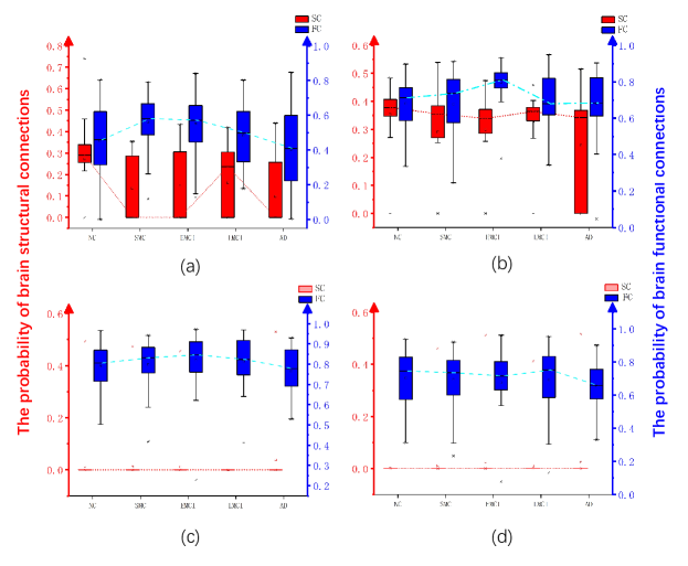
II Related Works

In recent years, more and more researchers have begun to use images of multiple modalities to explore the potential relationship between structure and function, especially how the emergence and disappearance of functional and structural connections interact each other. To tackle above difficulties, many models have been proposed to study AD-related knowledge with data of multiple modalities. Some models have been developed to learn the relationship between structure and function to explore the reason why a person’s brain structure is fixed in a certain period of time, but it can perform different functions.

Zhang et al. [25] recovered the structural connectivity via Multi-GCN from functional connectivity. The recovered result that functional information can predict structural information, revealed that functional information contains all the structural information. Wang et al. [26] proposed an algorithm called CDA and the empirical structural connections (SC) can be reliably predicted based on the direct anatomical relationships, indirect pathways, and module topology interact with one another forming temporally dependent functional connections (FC). Based on the fact that related brain regions with strong functional connectivity can exist without structural connectivity, but the strong functional connectivity can be observed in the brain regions with the strong structural connectivity, there is a many-to-one functional-structural mode.

However, it is not all researchers that agree with above views. Abdelnour et al [27] tried to use mathematical methods to derive a relationship between SC from DTI and FC from fMRI and found that using the approach via (structural) Laplacian spectral, FC and SC shared eigenvectors and their eigenvalues are exponentially related. Honey et al [28] believed that although resting state functional connectivity is variable, its strength, persistence and spatial statistics are constrained by the large-scale anatomical structure. Messé et al [29] explored the spatial consistency of the relationship between the structure and function of the human brain. The result showed that brain regions can affect the relationship between structural and functional connections. Different division methods will affect the relationship between structure and function. Simon et al [30] discussed the influence of different brain regions on structure and function and proved its effectiveness. Koch et al. [31] examined the correlation of spontaneous fluctuations of brain voxel BOLD signals in the cortical gyrus of the same hemisphere and found that there is a positive correlation between function and structure. Annen et al. [32] explore the relationship of function fluorodeoxyglucose FDG-PET metabolism and structure MRI-diffusion-weighted images (DWI). The fact that the patients’ local metabolism and white matter integrity were significantly reduced, showed that a stronger relationship of function-structure exists in most areas of Default mode network (DMN). Straathof et al. [33] combined multiple articles and draw a conclusion: the structural and functional connection strength of the mammalian brain is positively correlated with the connection strength of the diffuse structure on the macroscopic scale, and positively correlated with the connection strength of the neuron trace structure on the mesoscale.

Based on above analysis, the following simple assumption can be summarized: there is indeed a relationship between the structure and function. However, few people study the relationship between structure and function by employing complementary features between brain structure and function.

III Contributions

In this paper, a novel end-to-end framework named BGGAN is proposed where latent vector and graph information are effectively utilized and jointly optimized in both brain structural domain and functional domain. A hypothesis that there is some potential relationship between brain structure and function is proposed. To verify the validity of this hypothesis, a series of experiments are conducted to demonstrate the mapping from structural connection networks (SCN) to functional connection networks (FCN) and from FCN to SCN at the same time. Then the classification experiments are implemented to compare the classification results based on the data generated by BGGAN and the data generated by third-party software. Large differences between structure and function are found when conducting comparison experiments. Brain structure is relatively stable, and some structural abnormal brain connections are present in several comparison experiments. But it’s difficult to identify brain abnormal connections for brain function existing in above comparison experiments. Some brain regions obtained from the comparison experiments appeared multiple times.

The main contributions of this paper can be summarized as following:

• A novel framework called BGGAN is proposed by introducing the bidirectional mapping mechanism. Features of brain structure and brain function can be extracted mutually. Both the structural generator and functional generator can learn the complementary features between brain structure and brain function, which play a vital role in analyzing the relationship of brain structure-function.

• A new form of graph convolution named InnerGCN is designed. By extending graph convolution, the developed InnerGCN can deal with the third-order tensor while the traditional graph convolution can only process the brain connectivity matrix of a certain modality, namely second-order tensor. By extracting the features of different modalities using circle convolution mechanism, the InnerGCN can learn the brain structure-function features which are more close to the distribution of source domain.

• A new module named Balancer is proposed. By introducing the Balancer into BGGAN, the proposed model can not only alleviate the issue of mode collapse but also efficiently learn complementarity of structural and functional features. The generated connection with Balancer are more detailed and stable than that without Balancer.

The rest of this paper is organized as follows. In section IV, BGGAN is reviewed and the corresponding details for constructing the model are presented. In section V, the ADNI dataset is used to train the BGGAN model and perform bidirectional experiments between structure and function. The generated data is analyzed to reflect the changes of brain structure and function.

Figure 1: The proposed BGGAN involves two domain: structural domain and functional domain. BGGAN contains two extractors, two generators, two discriminators and two Balancer modules. The training steps are as following: (1) Firstly, extract the brain structural features based on sMRI and DTI data with structural extractor, and extract the functional features based on fMRI data with functional feature’s extractor. (2) Secondly, input the structural and functional features to structural and functional classifiers. The classification results are used to reflect the ability of the feature extractor and guide the learning of the extractors. (3) Thirdly, the structural and functional generators use the structural and functional feature matrices from the first step to perform bidirectional mapping between structural and functional domain. (4) Fourthly, the module Balancer merges the structural and functional connection matrices to reduce the gap between the source data and the target data. (5) Fifthly, structural and functional discriminators evaluate the differences between the generated data and the source data. The above steps describe the process from structure to function, and then reverse the generated function back to the structure. In fact, there is also the process of generating from function to structure, and then from structure to function, which is the same as before.

IV Method

IV-A Overview

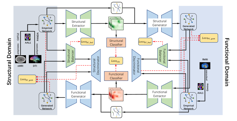
As show in Fig.1, the proposed framework consists of three modules: the Generator modules, the Discriminator modules and the Balancer modules. Generators contain feature extractors and brain connection generators. Feature extractors try to learn ninety brain regions’ features with multiple modalities. InnerGCN layers first utilize multiple modalities’ information more comprehensively. And then, the fully connected layers and the soft-max layers are appended behind the feature extractors to combine the multiple modalities’ features for classification. Good classification results can demonstrate that the InnerGCN layers can map the characteristics of different categories of subjects to corresponding areas in the latent space. The brain connection generators are then able to perform a bidirectional mapping between brain structure and function based on the features in the latent space. Discriminators are used to detect the authenticity between the generated data and the source data. The output of the discriminators is used to guide the generators to make the generated data distribution close to the source data distribution. The Balancer modules try to reduce the performance gap between the generators and the discriminators. The source data of the discriminator is doped with the information of empirical data from another domain through the Balancer module. Based on this, the gap between the generated data and the source data can be reduced, and the generators can learn the details of the source data distribution more smoothly.

The BGGAN can not only increase the model’s generalization effect, but also alleviate the modal crash issue. Unlike the traditional GAN model, BGGAN can generate the structural and functional connections at the same time. The Balancer designed in the BGGAN can assist them to balance the performance of the generators and discriminators in a more reasonable growth. The details of BGGAN are told in Section IV-B .

IV-B BGGAN for mapping domain

Generative adversarial networks [34, 35, 36, 37, 38] commonly consist of two modules: the module generator and the module discriminator. The generator tries to map latent features $z\sim p(z)$ from the noise or from the prior distribution to the distribution of the real domain. The discriminator aims to distinguish between the real data and the fake data. They are trained by the following min-max optimization Equation 1:

$$\begin{split}\min\limits_{G}\max\limits_{D}V(D,G)=\mathbb{E}_{x\sim p_{data}(x)}[logD(x)]+\\ \mathbb{E}_{z\sim p_{z}(z)}[log(1-D(G(z)))].\end{split}$$ (1)

Compared with traditional GAN framework using image convolution form, BGGAN in this paper uses the graph convolution as the calculation method. Just as shown in Fig.1, the input of generators is the brain connection matrices of multiple modalities, denoted as $\mathcal{G}=\{V,E\}$. $V\in\mathcal{R}^{N\times D\times R}$ and $E\in\mathcal{R}^{N\times N\times R}$. Here, $N$ is the number of brain regions, $D$ is the dimension of feature matrix and $R$ is the number of modalities. However, the traditional GCN method can not make full use of the information of multiple modal data. The input of traditional GCN can only be a matrix. When the input is multiple modalities data, parts of the information will be discarded. The traditional GCN method doesn’t take into account the relationship of different modalities. InnerGCN can utilize the relationship of multiple modalities and extract more comprehensive information. The details of InnerGCN will be introduced in section IV-C.

In addition, because of the instability of the traditional GAN framework and the unsmoothness of training process, the results of generators are very poor. The generated data are quite different with the source data. In view of above problems, the Balancer modules are add between the source data and the real input of discriminators, which can be seen in section IV-D in details. The loss function of the model can not only calculate the differences in brain region level, but also take into account the overall differences. The details of Balancer modules can be seen in section IV-E.

Based on above changes, BGGAN in this paper can realize the bidirectional mapping between structure and function at the same time by two generators and discriminators. The equations of BGGAN can be expressed in Eq.2.

$$\begin{split}\mathcal{L}_{GAN}=\mathcal{L}_{SC2FC}+\mathcal{L}_{FC2SC}+\mathcal{L}_{recon}\times\lambda\end{split}$$ (2)

Here, the $\mathcal{L}_{SC2FC}$ can be represented in Eq.3:

$$\begin{split}\mathcal{L}_{SC2FC}=\mathcal{L}_{cla}^{sc}+\mathcal{L}_{cons}^{fc}+\mathcal{L}_{recons}^{sc}+\mathcal{L}_{dis}^{fc}+\mathcal{L}_{dis}^{s}\\ =-\sum_{i=1}^{K}[y_{i}log(\hat{y_{i}}+(1-y_{i})\log(1-\hat{y_{i}}))]\\ +mse(real_{fc},gen_{fc})+mse(real_{sc},gen_{sc})\\ +dis(gen_{fc})+dis(gen_{sc}).\end{split}$$ (3)

and the $\mathcal{L}_{FC2SC}$ is same with the $\mathcal{L}_{SC2FC}$. $\mathcal{L}_{cla}^{sc}$ is the result of the classifier whose input is the generated data. $\mathcal{L}_{cons}^{fc}$ is the construction loss of the generator from SC to FC and $\mathcal{L}_{recons}^{sc}$ is the reconstruction loss of the generator from FC to SC. $\mathcal{L}_{dis}^{fc}$ is the output of the discriminator whose input is the generated and real brain functional networks, while $\mathcal{L}_{dis}^{sc}$ is the output of the discriminator whose input is the regenerated and real brain structural networks.

IV-C InnerGCN for extracting graphic features

Because of the topology of the brain, graph convolution networks have been widely used and achieved great results. Given a graph $G$ with an adjacency matrix $A\in\mathbb{R}^{N\times N}$, its diagonal degree matrix is represented as $D_{ii}=\sum_{j}A_{ij}$ and its normalized graph Laplacian can be denoted as $L=D^{-\frac{1}{2}}\hat{A}D^{-\frac{1}{2}}=I-D^{-\frac{1}{2}}AD^{-\frac{1}{2}}$, where $I$ is the identity matrix and $\hat{A}$ is the adjacency matrix $A$ with self-loop. And the realization of graph convolution can be expressed as the Eq.4:

$$\begin{split}X^{l+1}=\sigma(D^{-\frac{1}{2}}\hat{A}D^{-\frac{1}{2}}X^{l}W^{l}).\end{split}$$ (4)

where $H^{l}$ represents the input of the layer $l$ and $W^{l}$ is the weight matrix of layer $l$.

But traditional GCN can only use the single modal or utilize one modal as the connection matrix and the other as the feature matrix. Based on these methods, information of the modal cannot be made full use. Tensor product, referring to a multiple dimensional array of numbers, is a powerful tool to analyze multidimensional data[39, 40, 41]. Inspired from [42, 43, 44], we extend the input of graph convolution to high dimension space, which can utilize the features and connections of all modals at the same time.

First, some variables are defined first. $\mathcal{A}\in\mathbb{R}^{R\times N\times N}$ is the networks’ adjacency tensor, and features tensors of the brain networks can be defined as $X\in\mathbb{R}^{R\times N\times D}$. Here, $R$ is the modalities’ number of the input, $N$ is the brain regions’ number used in this paper and $D$ is the dimension of the features’ matrix. Due to the need of the formula below, we define $A(i)$ as $A(i)=A(i,:,:)$. And then the InnerGCN is as following:

$$\begin{split}x\star g=U^{H}\diamond((U\diamond x)\odot(U\diamond g)).\end{split}$$ (5)

where $x$ is the features’ tensor of the input and $g$ is the convolution kernel.

Next, we will introduce how to get $U$ in next steps: 1) get the Laplace tensor $L$, where $L(i)=I-D(i)^{-1/2}A(i)D(i)^{-1/2}$; 2) get the $L_{dft}$ from the $L$ in the Fourier form; 3) get the singular values matrix of each dimension of the tensor $[u(i),s(i)]=EVD(L_{dft}(i))$; 4) map the data in the Fourier data back to the original space $U=IDFT(u),\Lambda=IDFT(s)$. $U^{H}$ is the Hermitian matrix of $U$. $U\diamond x$ is the $U$ of Fourier form, and same as convolution filter $g$.

The third-order tensor can be considered as matrix with each element to be a vector. Same with matrix multiplication based on vector multiplication, matrix-matrix interaction is realized through circular convolution based on matrix multiplication. We defined $A,B$ as $A\in\mathbb{R}^{n_{1}\times n_{2}\times 3}$ and $B\in\mathbb{R}^{n_{2}\times n_{3}\times 3}$ and fold1(…), fold2(…), unfold(…) in Eq (6-9):

$$\begin{split}fold1(A)=\left[\begin{array}[]{cc}A_{1}\\ A_{2}\\ A_{3}\\ \end{array}\right]\end{split}$$ (6)

$$\begin{split}fold2(B)=\left[\begin{array}[]{ccc}B_{11}&B_{12}&B_{13}\\ B_{21}&B_{22}&B_{23}\\ B_{31}&B_{32}&B_{33}\\ \end{array}\right]\end{split}$$ (7)

$$\begin{split}unfold(\left[\begin{array}[]{ccc}B_{11}&B_{12}&B_{13}\\ B_{21}&B_{22}&B_{23}\\ B_{31}&B_{32}&B_{33}\\ \end{array}\right])=B\end{split}$$ (8)

$$\begin{split}A\diamond B=\mathcal{F}^{-1}(unfold(fold1(\mathcal{F}(A))\times fold2(\mathcal{F}(B))))\end{split}$$ (9)

In short, the process of InnerGCN is to Fourier transform the node features and the convolution kernel into the Fourier domain, and then let the two matrix multiply slice-by-slice in the Fourier domain, and finally inverse Fourier transform the result into the original space. It is circular convolution that makes the InnerGCN can nicely utilize relation correlations.

IV-D Balancer for smoothing training process of BGGAN

The basic idea of GAN is to train a nonlinear function, which can map the brain network from one domain to the other. To achieve this goal, the discriminator is trained to measure the distance of distribution between source and target data. The feedback of generators and discriminators can make generators learn mapping function from source domain to target domain.

In this paper, structural and functional brain networks are too distant from each other. Even if there is a similar mapping function between structural and functional domain, generators can not learn mapping function very well and details of the output can’t be generated. To decrease the distance between structural and functional domain, the Balancer is added between the real data of discriminator and the source data. The main idea of Balancer is to blur the real data of the discriminator and create a hyper-parameter to control the blurring level. As the epoch of training iterations increases, the generators of BGGAN gradually learn mapping function from the source domain to the target domain. Besides, since the ability of the discriminator is limited by the generator and the epoch of training epoch, the generators can gradually learn the details of the source data, making the output of the generator with Balancer much better than that without Balancer.

A neural network is utilized as Balancer, which is comprised of several convolution networks, a step connection combined the high order information and the low order information from the Balancer. Its loss function contains two parts: an adversarial loss $\mathcal{L}_{B}^{adv}$ and a reconstruction loss $\mathcal{L}_{B}^{recon}$. The function of the adversarial loss is to try fool the discriminator and slow down the discriminators’ learning process. The reconstruction loss is to limit the output similar to real sample and avoid the discriminator learn incorrect distribution too much. The Balancer is trained as following loss:

$$\begin{split}\mathcal{L}_{L}=\mathcal{L}_{L}^{adv}+\mathcal{L}_{L}^{recon}=-\mathcal{L}_{D}+\mathcal{L}_{L}^{recon}\\ =-D(\mathcal{X})+||\mathcal{X}-\mathcal{Y}||^{2}_{2}.\end{split}$$ (10)

where $\mathcal{X}$ is the input of Balancer, $\mathcal{Y}$ is the output of Balancer and $\mathcal{D}$ is a discriminator in the model.

To accelerate the training process, $\lambda$ is added in the loss function of Balancer. To have a smooth training procedure, $\lambda$ should be decreased gradually and the curve of $\lambda$’s values should be relatively smooth curve. After a certain training epochs, generators and discriminators have learned the relationship between the input and the output, Balancer should be deleted and make the model learn the details of the input. Considering above situation, the $\lambda$ is designed as shown in Eq(8):

$$\begin{split}\lambda=\left\{\begin{matrix}e^{-0.01t}&t\leq K\\ 0&t>K\end{matrix}\right.\end{split}$$ (11)

The $\lambda_{p}$ is obtained from the training procedure to normalize the $\lambda$ to between 1 and 2. Therefore, the overall loss of Balancer should be:

$$\begin{split}\mathcal{L}_{L}=\mathcal{L}_{L}^{adv}+\mathcal{L}_{L}^{recon}=-\lambda\mathcal{L}_{D}+\mathcal{L}_{L}^{recon}.\end{split}$$ (12)

In order to achieve above goals, we will design a new module named Balancer. It is mainly composed of convolution layers and ReLU activation layers. Because the input contains structural and functional information, the output of the balancer will contain both structural and functional information. Based on this, generators can learn structural and functional information at the same time.

IV-E Loss function for model

The loss function are composed by the following modules: 1) Classifier; 2) Generators; 3) Discriminators; 4) Balancers.

The overall loss function of the framework can be expressed as the following form:

$$\begin{split}\mathcal{L}=\mathcal{L}_{gan}+\mathcal{L}_{cons}+\mathcal{L}_{recon}+\mathcal{L}_{inden}+\mathcal{L}_{cla}.\end{split}$$ (13)

The $\mathcal{L}_{gan}$ is the output of the discriminator through calculating the distribution gap between generated and the source brain connections. The $\mathcal{L}_{cons}$ is the difference between generated data and the real data of source domain. The $\mathcal{L}_{recon}$ is the difference between reversely generated results and the real data of same domain. By means of calculating the generated results and real brain matrices of the original domain, the gap can be obtained and expressed as $\mathcal{L}_{index}$. The $\mathcal{L}_{cla}$ is obtained by the classifier to reflect the degree to which different types of features are mapped to different areas in the latent space.

Based on loss function 13, the model is gradually improved after each training epoch. Both the generated results and the classification results are optimized at the same time.

Algorithm 1 Bidirectional Inference algorithm on BGGAN

Input: each modalities’ feature information $F$, adjacency matrix $G$, subjects’ label $y$, maximum iterative number $EPOCH$ and hyperparameters $\lambda_{sc}$, $\lambda_{fc}$
  Output: structural and functional generated connections $G^{\prime}$ and model’s parameters $\Theta$

1:initialize model’s parameters $\Theta$, hyperparameters $\lambda_{sc}$, $\lambda_{fc}$ and $EPOCH$ = k, epoch = 0

2:for epoch $<$ EPOCH do

3:     epoch $\leftarrow$ epoch + 1

4:     update $\lambda$: $\lambda=e^{-0.01\times epoch}$ before epoch $<$ k

5:     combine structural and functional features and

6:          connectivity matrices($F_{sc}$, $E_{sc}$), ($F_{fc}$, $E_{fc}$)

7:     compute the latent feature of structure and function

8:          ($F^{\prime}_{sc}$, $F^{\prime}_{fc}$) by Equation: $U^{T}(Ux\odot Ug)$

9:     classify the subjects’ category based on ($F^{\prime}_{sc}$, $F^{\prime}_{fc}$)

10:     generate the structural and functional adjacency

11:          matrices: $E^{\prime}=F^{\prime}\times T(F^{\prime})$

12:     discriminate the generated structural and functional

13:          adjacency matrices:

14:          $\mathcal{L}^{\prime}_{gan}=Loss^{\prime}_{gen}+Loss^{\prime}_{dis}$

15:     recompute the latent feature of structure and function

16:          ($F^{\prime\prime}_{sc}$, $F^{\prime\prime}_{fc}$) by Equation: $U^{T}(Ux\odot Ug)$

17:     regenerate the structural and functional adjacency

18:          matrices : $E^{\prime\prime}=F^{\prime\prime}\times T(F^{\prime\prime})$

19:     rediscriminate the generated structural and

20:          functional adjacency matrices:

21:          $\mathcal{L}^{\prime\prime}_{gan}=Loss^{\prime\prime}_{gen}+Loss^{\prime\prime}_{dis}$

22:     compute the loss in the whole model:

23:          $\mathcal{L}_{cons}=||E,E^{\prime}||_{2}$

24:          $\mathcal{L}_{recon}=||E^{\prime},E^{\prime\prime}||_{2}$

25:          $\mathcal{L}_{inden}=||E,E^{\prime\prime}||_{2}$

26:          $\mathcal{L}_{gan}=L^{\prime}_{gan}+\mathcal{L}^{\prime\prime}_{gan}$

27:          $\mathcal{L}=\mathcal{L}_{gan}+\mathcal{L}_{cons}+\mathcal{L}_{recon}+\mathcal{L}_{inden}+\mathcal{L}_{cla}$

28:     update the parameters of the model:

29:          $\theta_{module}=\theta_{module}-\alpha\bigtriangledown_{\theta_{module}}L_{module}$

30:return generated brain functional and structural adjacency matrices

V Experiments

V-A Datasets

In this subsection, a series of experiments are conducted based on the Alzheimer’s Disease Neuroimaging Initiative (ADNI) datasets. ADNI began in 2004 under the leadership of Dr.Michael W.Weiner, funded as a private-public partnership with $27 million contributed by 20 companies and two foundations through the Foundation for the National Institutes of Health and $40 million from the National Institute on Aging. In our experiments, we used 80% subjects as training dataset, used 20% subjects as testing dataset. All experimental results are based on the testing dataset. The details of the datasets used in this paper are shown in Tab.I.

TABLE I: The situation of data used in the experiment

category	NC	SMC	EMCI	LMCI	AD
Number	153	94	135	63	64
Gender	81/72	35/59	86/49	35/28	39/25
Age	73.5$\pm$8.0	76.2$\pm$5.1	75.7$\pm$6.8	75.8$\pm$6.1	74.7$\pm$7.6
Weight	74.7$\pm$16.5	79.7$\pm$16.1	80.0$\pm$13.0	76.9$\pm$16.6	74.2$\pm$14.1

• The values are denoted as mean $\pm$ standard deviation. Categories contains Normal Control(NC), Significant Memory Concern(SMC), Early Mild Cognitive Impairment(EMCI), Late Mild Cognitive Impairment(LMCI) and Alzheimer’s Disease(AD).

V-B The effectiveness of InnerGCN

In this subsection, several comparison experiments are conducted to evaluate the effectiveness of InnerGCN. In order to control the redundant variables causing changes in the experimental results, we utilize the optimized parameters set and only change the InnerGCN to the rest graph convolution methods in this subsection. The hyperparameters of the model used in this section are defined in Tab.II.

TABLE II: The optimal parameters settings of the Model

parameter name	parameter value
Optimizer	Adaptive Moment Estimation(Adam)
Learning rate of Generators	0.0005
Learning rate of Discriminators	0.0005
Batch size	8
Stop Strategy	the early stop strategy
Number of ROIs	90
Types of Modality	sMRI,DTI,fMRI

Based on the above settings, three other comparison graph convolution methods, including GCN[45], GAE[46] and GAT[47] methods, are used to illustrate the effectiveness of InnerGCN. The classification indicators are used to assess these graph convolution methods’ performance.

Multiple sets of comparison experiments are used to validate the results achieved by InnerGCN in multiple modalities. Classification experiments are performed using multiple modalities’ fusion of fMRI and DTI data. For methods GCN, GAE and GAT, the node features are derived from the time series of fMRI, while the edge connection matrix are from the data of DTI. In addition, the InnerGCN takes both node features and edge connectivity information from fMRI and DTI data as model’s input.

The classification indicators $ACC$, $Recall$, $Precision$ and $F1\_score$ are used to evaluate the performance advantages and disadvantages with these different classification methods. These computational indicators are shown in Eq.(14-17).

• TP: Number of instances that are actually positive instances and classified as such by the classifier

• FP: Number of instances that are actually negative instances but classified as positive by the classifier

• FN: Number of instances that are actually positive but classified as negative by the classifier

• TN: Number of instances that are actually negative instances and classified as such by the classifier

$$\begin{split}ACC=\frac{TP+TN}{P+N}\end{split}$$ (14)

$$\begin{split}Recall=\frac{TP}{TP+FN}=\frac{TP}{P}\end{split}$$ (15)

$$\begin{split}Precision=\frac{TP}{TP+FP}\end{split}$$ (16)

$$\begin{split}F_{1}\_score=\frac{2\times Precision\times Recall}{Precision+Recall}\end{split}$$ (17)

Figure 2: Classification performance based on different graph convolution methods. GCN, GAE and GAT set the brain structural information as the edges of graph and the brain functional information as the node features of graph. The classification result based on our method reaches best.

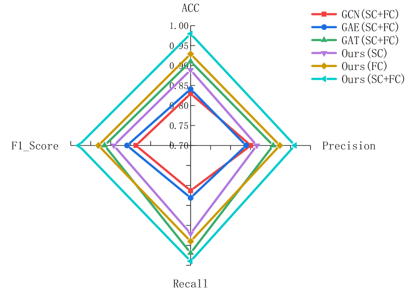
As shown in Fig.2, both GAT and InnerGCN show a great improvement in classification results compared with other graph convolution methods. However, InnerGCN can better utilize the complementary information between these two multiple modal data, which improves the classification accuracy greatly and proves the validity of the InnerGCN.

V-C The effectiveness of the Balancer

In fact, generative adversarial networks are subject to significant instabilities. In the models like ours, discriminators tend to reach the optimal case more quickly than generators, which leaves a great performance divide between discriminators and generators in same model.

To tackle this problem, the training speed of the discriminator need to slow down and the gap between source domain and target domain should be reduced. In other words, retarding the optimization process of the discriminator makes the generator’s training more stable.

To weight these important factors above, a new module named Balancer is proposed and added between source data and discriminators. Before adding the module, the source data is directly inputted to the discriminator. In order to retard the learning speed of the discriminator and try to improve the performance of the generator step by step, the source domain and target domain are integrated together into the input of the discriminator until multiple epochs pasted.

Figure 3: (a) shows the MSE loss between the target and the source domain connections. The orange curve is the loss outputted by the generator without module Balancer, while the green curve is the loss with module Balancer. (b) shows the generated structural connections from the functional generator. The top five pictures are the results from the generator without module Balancer and the bottom five are the results from the generator with module Balancer.

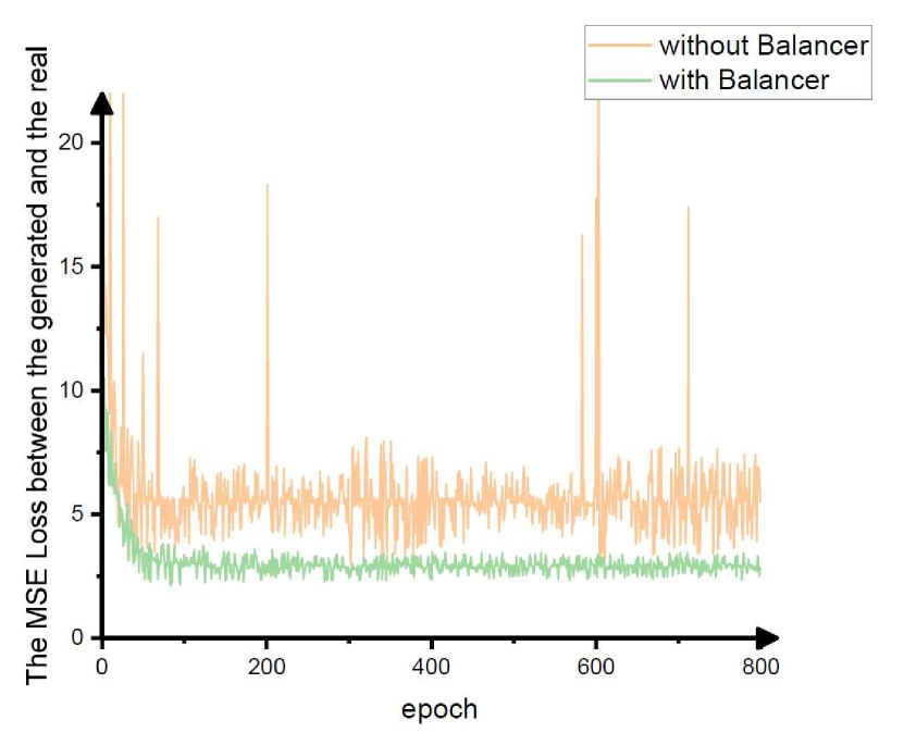
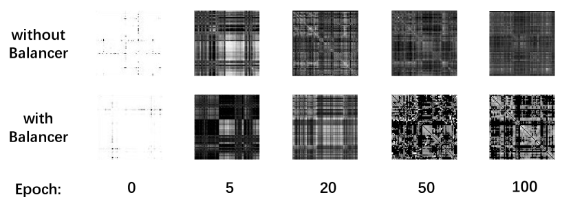
Here we conduct two sets of comparison experiments, one without Balancer and one with Balancer. From Fig.3, it is clear that there is a large difference in the loss of the functional generator in two cases. The generator with module Balancer has better training results and the training process is more stable, while the generator without module Balancer can reach a better level faster at the beginning of training. Based on the model without module Balancer, the discriminator reaches a better level soon. As a result, although discriminators’ grade is more accurate, the generators’ next training will be more difficult instead. When the training process reaches a certain level, the generator has learned some distributions. The training of the discriminator should also change with the training process of the generator. Just as shown in Fig.3, the top five pictures show generated brain functional connections without module Balancer and the bottom five pictures are the generated brain functional connections with the module Balancer. Although good results can be achieved regardless of whether the module Balancer is used or not, the results tell us that the generated results with the Balancer get more realistic details as well.

V-D The connection number changes from NC and AD in structural and functional domain

Although many articles have stated that structure is the basis of function, there is actually a huge difference between structure and function in terms of brain analysis performance.

In this section, we will discuss differences of brain structure and function in terms of the number of brain connections. In order to reflect the relationships between brain structure and function, we compared the brain connection number changes in structure and function from NC to AD.

Figure 4: Statistical analysis for structural and functional brain connections under each category. The figure (a) shows the number trend of structural connections and the figure (b) shows the number trend of functional connections.

Figure 5: Similarities and differences between brain structural connections and brain functional connections in each category. The brighter the plot, the higher the probability of presence of brain connections. The yellow areas indicate a higher likelihood of brain connections, while the rest of the purple colors indicate that brain connections are less likely to be present. Top five figures show brain connections where structural connections usually exist but functional connections do not. The five figures in the middle show the brain connections that have a high probability of function but rarely structure. And the bottom five show brain connections that both exist multiple times in structure and function.

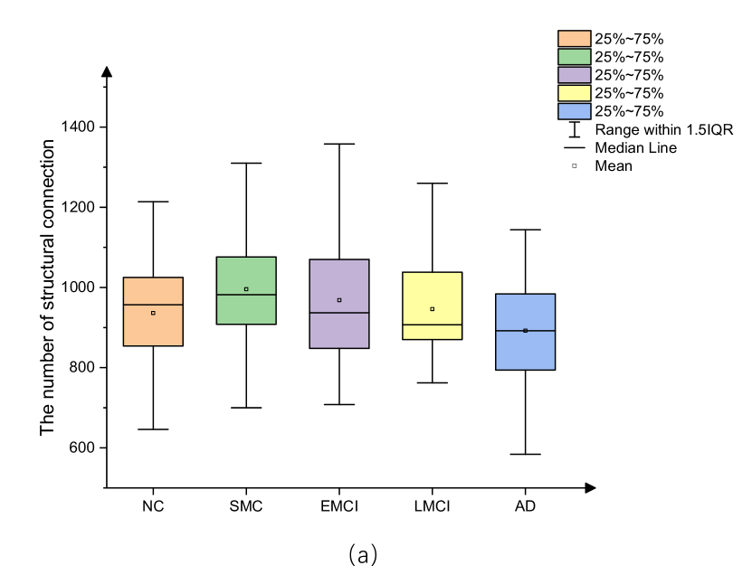
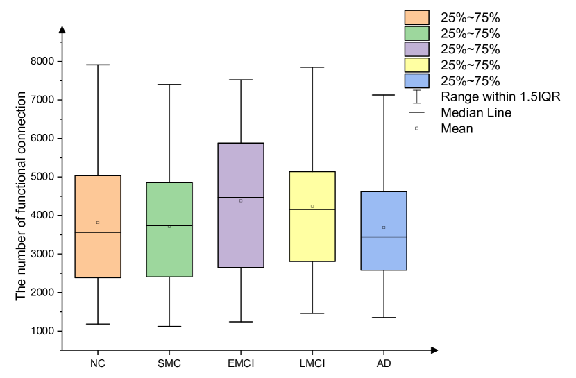
Then structural and functional brain connections are compared in the large aspect of the same category. 60 subjects in each category are identified for generating structural and functional brain connections. Then the number of structural connections and the number of functional connections are counted. The statistical results are shown in Fig.4. As shown in Fig.4 and Fig.4, the number of structural brain connections increased first and then decreased. This situation is same as the functional brain connections. This also confirms that Alzheimer’s disease does have a strong relationship with the number of brain structural and functional connections. The difference is that the start of the decline in the number of structural brain connections occurs at SMC, whereas the decline in the number of functional brain connections occurs at the EMCI stage, a later stage of SMC. Maybe, the greater coordination of the functional brain domains and the relatively more stable structure of the brain allowed the growth of functional brain connectivity to not begin to decline until the EMCI stage.

V-E The brain adjacency changes from NC to AD

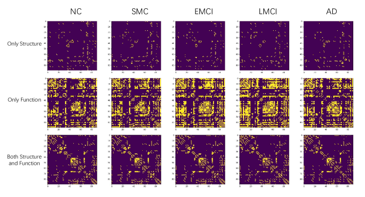
Then, we compared the differences in brain structure and function under the perspective of brain regions. Here, we performed multiple comparison experiments using the averaging method, including {NC vs. SMC, NC vs. EMCI, NC vs. LMCI, NC vs. AD}. Fig.5 shows the comparative results of these experiments.

The results in Fig.5 are calculated in Independent Samples t-Test method based on brain generated structural and functional connections which are synthesized by trained generators above. The top five diagrams show brain connections where structure is often present but function is infrequent; the middle five diagrams show brain connections where function occurs many times but structure rarely; and the bottom five diagrams show brain connections where both structure and function occur with high probability. The brighter the plot, the higher the probability of the presence of brain connections. There are similarities in the data distribution in each row as a whole, but there are huge differences in some regions.

Based on above comparison experiments, functional brain connections tend to occur between brain regions that are directly connected to brain structures, and conversely, brain regions with functional brain connections are not necessarily directly connected to each other by structural brain connections. However, the fact is that the number of brain functional connections is much larger than that of brain structural connections. There are also brain functional connections between many brain regions that do not have brain structural connections. We can reasonably speculate that functional brain connections may be the result of multiple brain regions acting together to achieve the corresponding functions.

To further prove the above conclusion, three subjects’ structural and functional brain connections from each category are selected to obtain the similarities and differences between structural and functional brain connections.

Figure 6: This figure shows the similarities and differences of five categories at the individual level. The red indicates brain connections with a high probability of both structure and function, the green indicates brain connections with frequent function but little structure, and the blue is brain connections with frequent structure but little function, and white indicates a small probability of both structure and function.

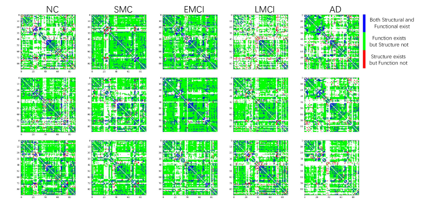
In Fig.6, it is clear that even within the same category, there are large differences between structure and function, but most of them have the following conclusions: 1) there are fewer brain connections where both brain structure and brain function are present, and their locations are more fixed; 2) there are relatively few regions where only brain structure connections are present, and some of them are present in all categories; 3) the regions where only brain function connections are present occupy a larger area.

Comparing the above two figure, there is a one-to-one correspondence between structure and function in some connections, but on a larger scale there is not a one-to-one correspondence between structural and functional brain connections. Brain structure is the basis of brain function, demonstrating that there are complex relationships in the brain that allow information transfer between brain regions without structural connections to perform the corresponding functions.

V-F Differences of brain adjacency matrices in different categories compared with NC

In this section, 60 subjects’ data from each category are randomly selected in this experiment. The brain structural and functional adjacency matrices based on the Independent Samples t-Test method is conducted to obtain the difference in haunting relationships between patients and normal subjects.

Figure 7: The p-value results based on the Independent Samples t-Test of structure and function under adjacent categories compared with normal control. The top four images are structural comparison results and the bottom four images are functional comparison results.

According to Fig.7, the more yellow the color, the greater the p-value, which means that adjacent categories will have brain connections present between these two brain regions. It can be clearly seen that the structural changes are less than the functional during the progression of the disease. But the changes of structure and function are almost in similar adjacent brain regions.

Figure 8: (a) shows the brain abnormal connection between brain region 85 and 87, (b) shows the brain abnormal connection between brain region 52 and 54; while (c) shows the brain normal connection between brain region 83 and 84, (d) is the brain normal connection between brain region 85 and 86.

TABLE III: Top 30 abnormal brain connections obtained using Independent Samples t-Test experiments compared to normal subjects. The numbers in this table represent brain area number.

SMC vs. NC		EMCI vs. NC		LMCI vs. NC		AD vs. NC
SC	FC	SC	FC	SC	FC	SC	FC
40-56	56-88	6-31	50-87	40-56	37-61	85-87	28-76
46-47	55-88	4-30	49-76	6-27	6-25	52-86	69-75
73-82	41-88	46-47	50-76	6-31	14-23	37-82	20-75
47-48	76-77	14-78	58-87	6-25	3-76	65-85	28-75
85-87	44-75	29-71	87-90	12-62	63-65	37-87	2-17
47-68	68-76	86-88	50-80	4-30	30-72	7-83	49-65
19-29	43-76	85-87	5-70	5-6	57-61	39-87	8-61
60-62	51-76	38-43	5-38	4-73	2-76	53-89	34-45
52-54	41-53	30-72	60-65	4-75	23-29	41-87	75-76
48-54	41-55	6-32	51-76	38-55	69-76	63-85	2-75
38-82	43-75	88-90	57-87	41-71	36-53	7-23	6-75
33-73	44-76	41-87	44-87	77-78	9-38	48-54	79-90
2-30	47-76	14-77	49-87	23-51	63-69	52-54	29-64
44-47	75-77	8-24	30-71	58-59	56-88	38-88	49-66
9-31	67-76	34-77	16-69	85-87	22-76	35-85	16-76
44-86	46-76	40-56	14-60	25-71	38-62	7-31	31-35
48-67	41-89	6-76	43-87	30-62	50-62	47-50	52-75
36-48	16-41	4-76	59-65	30-31	38-61	53-55	54-62
38-84	42-88	32-78	54-87	4-68	43-57	77-78	5-15
30-72	50-55	14-24	52-76	7-78	58-62	55-87	17-58
1-29	25-27	32-33	4-69	59-82	1-76	40-88	2-64
41-87	51-87	80-86	52-87	22-78	2-36	35-81	2-62
33-82	56-87	1-83	6-44	2-86	43-69	42-88	72-89
29-68	15-56	34-37	44-76	10-73	2-3	29-34	35-44
29-33	52-55	40-88	9-55	30-73	57-89	52-90	58-64
43-74	43-87	39-78	17-58	35-74	61-69	72-88	1-75
78-84	9-75	87-89	30-65	4-77	4-76	29-57	35-47
37-78	42-54	52-54	49-80	5-78	1-43	60-78	57-75
52-60	42-51	33-51	15-56	29-68	10-23	10-42	52-65
74-77	49-87	7-78	51-87	25-78	1-44	4-19	25-35

Based on above four comparison results, we further counted the first 30 abnormal brain connections lower than 0.05 in these experiments compared to normal subjects, and the results are shown in the Tab.III. From the table, a clear phenomenon can be found: there were multiple abnormal brain connections in the structural experiments, and these brain connections appeared many times in these four groups of experiments, while there were no such abnormal brain connections in the functional experiments, or at most in two groups of experiments. This proves that the deterioration of brain structure is gradual, but through its coordination mechanism, the brain can skip the original abnormal brain connections, use other connections to achieve the same task, which are different with the brain connections of NC.

By comparing these first 30 brain connections, just shown in Tab.III, it was found that the structural data is relatively stable, such as the brain connections between brain region Occipital_Mid_R and Occipital_Inf_R or brain region Temporal_Mid_L and Temporal_Pole_Mid_L, appeared many times in these four groups of experiments. For this reason, we utilized 60 subjects and counted the connection strength of their brain connections between brain region Temporal_Mid_L and Temporal_Pole_Mid_L, and between brain region Occipital_Mid_R and Occipital_Inf_R. The statistical result is shown in Fig.8. Fig.8(a) and Fig.8(b) are the abnormal brain connections’ results, while Fig.8(c) and Fig.8(d) are the normal brain connections’ results. Abnormal brain connections exhibit more instability than normal brain connections in structure domain. Different with the brain normal connections, the curves of the abnormal connection between brain region Occipital_Mid_R and Occipital_Inf_R, or brain region Temporal_Mid_L and Temporal_Pole_Mid_L show a large degree of amplitude change. And it demonstrates that the abnormal situation got from the experiments are much different with the normal connection. The abnormal brain connections in {40-56, 85-87, 52-54, 30-72, 41-87} have the same change trend.

However, compared with structural data, functional data showed more abnormal results in some brain regions. Among all brain regions, brain regions {76, 87, 75, 44, 43, 69, 2, 49, 65} appeared with much frequency. We used BrainNetViewer[48] to organize all these abnormal brain connections and brain regions in Fig.9 and in Fig.10.

Figure 9: Abnormal brain structural and functional connections that are present in these comparison experiments.

Figure 10: Abnormal brain structural and functional regions that are present multiple times in these comparison experiments.

VI Discussion

In the above experiments, we compared the differences between structural and functional connections. When comparing brain structural and functional connection matrices at the individual level, there is not a simple one-to-one correspondence between brain structural and functional connections. There is a high probability that the brain regions with structural connections also have functional connections. However, the brain regions with functional connections do not necessarily have structural connections. It indicates that direct brain structural connectivity does not necessarily have to exist between brain regions that can transmit information and multiple direct brain structural connections can assist in forming indirect brain structure connections to achieve the corresponding functions.

When comparing brain structural and functional connection matrices at the category level, there are large differences in the abnormalities obtained in structure and function. Structural abnormalities were relatively stable. There are some abnormal brain connections existing in all comparative experiments, but there is no function. There are no abnormal brain connections mentioned above, but there are many abnormal brain regions existing in these comparative experiments.

There are still some problems that are not solved in this paper. Although the correspondence between structure and function can be imitated by generators, the specific correspondence between the structure and function, i.e., the coordination mechanism of the brain, remains ungraspable. Some subjects have large differences compared to the same category of subjects, and how they should go about the diagnosis.

VII Conclusion

In this paper, we proposed a new graph convolution method, called InnerGCN, to map the structural and functional brain networks of human brain to each other. And two generators and discriminators learn the structure-to-function and function-to-structure mapping function, respectively. However, direct comparison of structure and function doesn’t not reveal similarities between structure and function, suggesting that there is not a one-to-one correspondence between structure and function, but rather a complex coordination mechanism. In addition, we compared the structural and functional connectivity of the patients during the deterioration of the disease AD. The structural data yielded more stable abnormal brain connections, while the functional data yielded abnormal brain connections that were difficult to detect as such, but many of these connections were connected to some specified brain regions.

References

- [1] Liana G Apostolova. Alzheimer disease. Continuum: Lifelong Learning in Neurology, 22(2 Dementia):419, 2016.
- [2] Martin Citron. Alzheimer’s disease: strategies for disease modification. Nature reviews Drug discovery, 9(5):387–398, 2010.
- [3] Michel Goedert and Maria Grazia Spillantini. A century of alzheimer’s disease. science, 314(5800):777–781, 2006.
- [4] Zaven S Khachaturian. Diagnosis of alzheimer’s disease. Archives of neurology, 42(11):1097–1105, 1985.
- [5] Mark P Mattson. Pathways towards and away from alzheimer’s disease. Nature, 430(7000):631–639, 2004.
- [6] Lennart Mucke. Alzheimer’s disease. Nature, 461(7266):895–897, 2009.
- [7] Tong Tong, Katherine Gray, Qinquan Gao, Liang Chen, Daniel Rueckert, Alzheimer’s Disease Neuroimaging Initiative, et al. Multi-modal classification of alzheimer’s disease using nonlinear graph fusion. Pattern recognition, 63:171–181, 2017.
- [8] Prashanthi Vemuri and Clifford R Jack. Role of structural mri in alzheimer’s disease. Alzheimer’s research & therapy, 2(4):1–10, 2010.
- [9] D Zhang and D Shen. Alzheimer’s disease neuroimaging i. multi-modal multi-task learning for joint prediction of multiple regression and classification variables in alzheimer’s disease. NeuroImage, 59(2):895–907, 2012.
- [10] Shuqiang Wang, Hongfei Wang, Yanyan Shen, and Xiangyu Wang. Automatic recognition of mild cognitive impairment and alzheimers disease using ensemble based 3d densely connected convolutional networks. In 2018 17th IEEE International conference on machine learning and applications (ICMLA), pages 517–523. IEEE, 2018.
- [11] Shuqiang Wang, Yanyan Shen, Wei Chen, Tengfei Xiao, and Jinxing Hu. Automatic recognition of mild cognitive impairment from mri images using expedited convolutional neural networks. In International Conference on Artificial Neural Networks, pages 373–380. Springer, 2017.
- [12] Karim Aderghal, Jenny Benois-Pineau, and Karim Afdel. Classification of smri for alzheimer’s disease diagnosis with cnn: single siamese networks with 2d+? approach and fusion on adni. In Proceedings of the 2017 ACM on International Conference on Multimedia Retrieval, pages 494–498, 2017.
- [13] Abol Basher, Byeong C Kim, Kun Ho Lee, and Ho Yub Jung. Volumetric feature-based alzheimer’s disease diagnosis from smri data using a convolutional neural network and a deep neural network. IEEE Access, 9:29870–29882, 2021.
- [14] Baiying Lei, Mengya Yang, Peng Yang, Feng Zhou, Wen Hou, Wenbin Zou, Xia Li, Tianfu Wang, Xiaohua Xiao, and Shuqiang Wang. Deep and joint learning of longitudinal data for alzheimer’s disease prediction. Pattern Recognition, 102:107247, 2020.
- [15] Hongfei Wang, Yanyan Shen, Shuqiang Wang, Tengfei Xiao, Liming Deng, Xiangyu Wang, and Xinyan Zhao. Ensemble of 3d densely connected convolutional network for diagnosis of mild cognitive impairment and alzheimer’s disease. Neurocomputing, 333:145–156, 2019.
- [16] Shuqiang Wang, Hongfei Wang, Albert C Cheung, Yanyan Shen, and Min Gan. Ensemble of 3d densely connected convolutional network for diagnosis of mild cognitive impairment and. Deep learning applications, 1098:53, 2020.
- [17] Senrong You, Baiying Lei, Shuqiang Wang, Charles K Chui, Albert C Cheung, Yong Liu, Min Gan, Guocheng Wu, and Yanyan Shen. Fine perceptive gans for brain mr image super-resolution in wavelet domain. IEEE transactions on neural networks and learning systems, 2022.
- [18] Shuqiang Wang, Xiangyu Wang, Yong Hu, Yanyan Shen, Zhile Yang, Min Gan, and Baiying Lei. Diabetic retinopathy diagnosis using multichannel generative adversarial network with semisupervision. IEEE Transactions on Automation Science and Engineering, 18(2):574–585, 2020.
- [19] Wen Yu, Baiying Lei, Shuqiang Wang, Yong Liu, Zhiguang Feng, Yong Hu, Yanyan Shen, and Michael K Ng. Morphological feature visualization of alzheimer’s disease via multidirectional perception gan. IEEE Transactions on Neural Networks and Learning Systems, 2022.
- [20] MM Machulda, HA Ward, B Borowski, JL Gunter, RH Cha, PC O’brien, RC Petersen, BF Boeve, D Knopman, DF Tang-Wai, et al. Comparison of memory fmri response among normal, mci, and alzheimer’s patients. Neurology, 61(4):500–506, 2003.
- [21] Liang Wang, Yufeng Zang, Yong He, Meng Liang, Xinqing Zhang, Lixia Tian, Tao Wu, Tianzi Jiang, and Kuncheng Li. Changes in hippocampal connectivity in the early stages of alzheimer’s disease: evidence from resting state fmri. Neuroimage, 31(2):496–504, 2006.
- [22] Junren Pan, Baiying Lei, Shuqiang Wang, Bingchuan Wang, Yong Liu, and Yanyan Shen. Decgan: Decoupling generative adversarial network detecting abnormal neural circuits for alzheimer’s disease. arXiv preprint arXiv:2110.05712, 2021.
- [23] Talia M Nir, Neda Jahanshad, Julio E Villalon-Reina, Arthur W Toga, Clifford R Jack, Michael W Weiner, Paul M Thompson, Alzheimer’s Disease Neuroimaging Initiative (ADNI, et al. Effectiveness of regional dti measures in distinguishing alzheimer’s disease, mci, and normal aging. NeuroImage: clinical, 3:180–195, 2013.
- [24] Kenichi Oishi, Michelle M Mielke, Marilyn Albert, Constantine G Lyketsos, and Susumu Mori. Dti analyses and clinical applications in alzheimer’s disease. Journal of Alzheimer’s Disease, 26(s3):287–296, 2011.
- [25] Lu Zhang, Li Wang, and Dajiang Zhu. Recovering brain structural connectivity from functional connectivity via multi-gcn based generative adversarial network. In International Conference on Medical Image Computing and Computer-Assisted Intervention, pages 53–61. Springer, 2020.
- [26] Yanjiang Wang, Xue Chen, Baodi Liu, Weifeng Liu, and Richard Martin Shiffrin. Understanding the relationship between human brain structure and function by predicting the structural connectivity from functional connectivity. IEEE Access, 8:209926–209938, 2020.
- [27] Farras Abdelnour, Michael Dayan, Orrin Devinsky, Thomas Thesen, and Ashish Raj. Functional brain connectivity is predictable from anatomic network’s laplacian eigen-structure. NeuroImage, 172:728–739, 2018.
- [28] Christopher J Honey, Olaf Sporns, Leila Cammoun, Xavier Gigandet, Jean-Philippe Thiran, Reto Meuli, and Patric Hagmann. Predicting human resting-state functional connectivity from structural connectivity. Proceedings of the National Academy of Sciences, 106(6):2035–2040, 2009.
- [29] Arnaud Messé. Parcellation influence on the connectivity-based structure–function relationship in the human brain. Human brain mapping, 41(5):1167–1180, 2020.
- [30] Andrew F Leuchter, Ian A Cook, Sebastian HJ Uijtdehaage, Jennifer Dunkin, Robert B Lufkin, Catherine Anderson-Hanley, Michelle Abrams, Susan Rosenberg-Thompson, Ruth O’Hara, Sara L Simon, et al. Brain structure and function and the outcomes of treatment for depression. Journal of Clinical Psychiatry, 58(16):22–31, 1997.
- [31] Martin A Koch, David G Norris, and Margret Hund-Georgiadis. An investigation of functional and anatomical connectivity using magnetic resonance imaging. Neuroimage, 16(1):241–250, 2002.
- [32] Jitka Annen, Lizette Heine, Erik Ziegler, Gianluca Frasso, M Bahri, Carol Di Perri, Johan Stender, Charlotte Martial, Sarah Wannez, Kevin D’ostilio, et al. Function–structure connectivity in patients with severe brain injury as measured by mri-dwi and fdg-pet. Human brain mapping, 37(11):3707–3720, 2016.
- [33] Milou Straathof, Michel RT Sinke, Rick M Dijkhuizen, and Willem M Otte. A systematic review on the quantitative relationship between structural and functional network connectivity strength in mammalian brains. Journal of Cerebral Blood Flow & Metabolism, 39(2):189–209, 2019.
- [34] Wen Yu, Baiying Lei, Michael K Ng, Albert C Cheung, Yanyan Shen, and Shuqiang Wang. Tensorizing gan with high-order pooling for alzheimer’s disease assessment. IEEE Transactions on Neural Networks and Learning Systems, 2021.
- [35] Shengye Hu, Wen Yu, Zhuo Chen, and Shuqiang Wang. Medical image reconstruction using generative adversarial network for alzheimer disease assessment with class-imbalance problem. In 2020 IEEE 6th International Conference on Computer and Communications (ICCC), pages 1323–1327. IEEE, 2020.
- [36] Shuangzhi Yu, Shuqiang Wang, Xiaohua Xiao, Jiuwen Cao, Guanghui Yue, Dongdong Liu, Tianfu Wang, Yanwu Xu, and Baiying Lei. Multi-scale enhanced graph convolutional network for early mild cognitive impairment detection. In International Conference on Medical Image Computing and Computer-Assisted Intervention, pages 228–237. Springer, Cham, 2020.
- [37] Qiankun Zuo, Baiying Lei, Yanyan Shen, Yong Liu, Zhiguang Feng, and Shuqiang Wang. Multimodal representations learning and adversarial hypergraph fusion for early alzheimer’s disease prediction. In PRCV2021, number 13021, pages 479–490, 2021.
- [38] Junren Pan, Baiying Lei, Yanyan Shen, Yong Liu, Zhiguang Feng, and Shuqiang Wang. Characterization multimodal connectivity of brain network by hypergraph gan for alzheimer’s disease analysis. In PRCV2021, number 13021, pages 467–478, 2021.
- [39] Michaek Kwok-Po Ng, Xutao Li, and Yunming Ye. Multirank: co-ranking for objects and relations in multi-relational data. In Proceedings of the 17th ACM SIGKDD international conference on Knowledge discovery and data mining, pages 1217–1225, 2011.
- [40] Xutao Li, Michael K Ng, and Yunming Ye. Multicomm: Finding community structure in multi-dimensional networks. IEEE Transactions on Knowledge and Data Engineering, 26(4):929–941, 2013.
- [41] Xutao Li, Yunming Ye, and Xiaofei Xu. Low-rank tensor completion with total variation for visual data inpainting. In Proceedings of the AAAI Conference on Artificial Intelligence, volume 31, 2017.
- [42] Zhichao Huang, Xutao Li, Yunming Ye, and Michael K Ng. Mr-gcn: Multi-relational graph convolutional networks based on generalized tensor product. In IJCAI, pages 1258–1264, 2020.
- [43] Misha E Kilmer and Carla D Martin. Factorization strategies for third-order tensors. Linear Algebra and its Applications, 435(3):641–658, 2011.
- [44] Guangjing Song, Michael K Ng, and Xiongjun Zhang. Robust tensor completion using transformed tensor singular value decomposition. Numerical Linear Algebra with Applications, 27(3):e2299, 2020.
- [45] Thomas N Kipf and Max Welling. Semi-supervised classification with graph convolutional networks. arXiv preprint arXiv:1609.02907, 2016.
- [46] Thomas N Kipf and Max Welling. Variational graph auto-encoders. arXiv preprint arXiv:1611.07308, 2016.
- [47] Petar Veličković, Guillem Cucurull, Arantxa Casanova, Adriana Romero, Pietro Lio, and Yoshua Bengio. Graph attention networks. arXiv preprint arXiv:1710.10903, 2017.
- [48] M. Xia, J. Wang, and H. Yong. Brainnet viewer: A graph-based brain network mapping tool. 2011.