Stochastic Schrödinger equation approach to real-time dynamics of Anderson-Holstein impurities: an open quantum system perspective

Zhen Huang Department of Mathematics, University of California, Berkeley, CA 94720, USA    Limin Xu Department of Mathematical Sciences, Tsinghua University, Beijing 100084, China    Zhennan Zhou zhennan@bicmr.pku.edu.cn Beijing International Center for Mathematical Research, Peking University, Beijing, 100871, China
Abstract

We develop a stochastic Schrödinger equation (SSE) framework to simulate real-time dynamics of Anderson-Holstein (AH) impurities coupled to a continuous fermionic bath. The bath degrees of freedom are incorporated through fluctuating terms determined by exact system-bath correlations, which is derived in an ab initio manner. We show that such an SSE treatment provides a middle ground between numerically expansive microscopic simulations and macroscopic master equations. Computationally, the SSE model enables efficient numerical methods for propagating stochastic trajectories. We demonstrate that this approach not only naturally provides microscopically-detailed information unavailable from reduced models, but also captures effects beyond master equations, thus serves as a promising tool to study open quantum dynamics emerging in physics and chemistry.

I Introduction

Real-time dynamics of quantum impurity systems with fermionic baths have been a central topic in condensed matter physics for the past few decades. It is used to model a wide range of systems, such as magnetic impurities in metals [1], quantum dot systems [2], atom adsorption onto surface [3]. Among various types of quantum impurity models, the Anderson-Holstein (AH) model [4, 5] is of critical importance, since it is directly related to chemisorption [4], electrochemistry [6], heterogeneous catalysis [7] and molecular junctions [8].

The Anderson-Holstein model comprises of a molecular system as the impurity part and the continuous heat bath equilibrated at a certain temperature as the environment. For example, when modeling molecule-metal interfaces, the bath part is made up of metal orbitals of a continuum of spectra [4, 5]. The most straightforward simulation strategy would be a direct discretization of the bath orbitals (for example, see [9, 10]), and then propagate the many-body Schrödinger equation for the entire extended system. However, such calculations are often so expensive that either one is only capable of studying a model with a very small number of bath orbitals [11], or one makes crude single-particle approximations [12]. These treatments are far from exact and are only effective in limited scenarios.

The impurities could be viewed as a fermionic open quantum system due to the influence of the infinite bath. To incorporate the open-system effects with a manageable computational cost, various master equations are developed based on different physical approximations. This is generally seen in the study of molecular-metal interfaces. Treating the nuclei of the molecular system as classical particles, classical master equations (CME) [13, 14] are proposed along with surface hopping technique [15, 16] to efficiently sample the ensemble at equilibrium. However, due to the breakdown of the Born-Oppenheimer approximation, it is necessary to capture the nuclear quantum effects and nonadiabatic dynamics simultaneously. This is often achieved by quantum master equations (QME), which describe the dynamics for the reduced density matrix by tracing out the electronic degree of freedom. Lindblad master equations [17, 18] are used when one makes the Markovian approximation. To capture the memory effects, Nakajima-Mori-Zwanzig equations [19, 20], Redfield equations [21, 22] and other non-Markovian equations [23, 24, 25] are proposed as effective models. QME is widely used to model realistic systems [25, 26, 24, 27]. The hierarchy quantum master equation (HQME) [28, 29, 27], also known as the hierarchy equation of motion (HEOM), is a nonperturbative alternative but is often computationally too expensive.

However, there is another widely-used approach, namely Stochastic Schrödinger equations (SSE), for studying open quantum systems. By incorporating stochastic fluctuations arising from interactions with the external environment, SSE has been successfully used in modeling quantum decoherence[30, 31], quantum measurement [32, 33, 34], quantum jumps [35, 36] and so on. It is found to be consistent with QME calculations in many cases [37, 38, 39, 40], and in the meantime has the following additional advantages: on the one hand, SSE provides an ensemble of time-dependent quantum trajectories, and therefore is very convenient for studying the statistical and nonequilibrium properties of the open system; on the other hand, the numerical methods for simulating stochastic differential equations have already been studied extensively [41, 42], and as a result the above trajectories could be obtained effectively with a Monte-Carlo sampling scheme. However, the success of SSE models highly relies on the accurate modeling of the environment, i.e. obtaining the exact time-correlation function of the noise term in SSE.

Even though SSE is a very powerful tool in the modeling of open quantum systems, it has not been applied to study the real-time dynamics of quantum impurities with fermionic bath, to the best of our knowledge. On the one hand, SSE approaches are mostly developed for bosonic heat bath in different regimes. On the other hand, although there are attempts of using SSE to study fermionic bath effects [37, 43], there lacks an ab initio treatment of the stochastic and non-Markovian effects, therefore not applicable to general chemical systems such as molecule-metal interfaces.

The purpose of this article is two-fold. On the one hand, we aim to fill in a gap in the study of Anderson-Holstein models as an open quantum system: the time-correlation function of the noise term in SSE is obtained directly from the Anderson-Holstein Hamiltonian. On the other hand, we emphasize the following hierarchy of modeling: SSE is at an intermediate level of approximation, right between the atomic-level AH model and the QME model:

Anderson-HolsteinSSEQME.Anderson-HolsteinSSEQME\text{Anderson-Holstein}\rightarrow{\mathrm{SSE}}\rightarrow\mathrm{QME}.

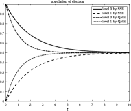
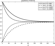
For a detailed description of this modeling hierarchy, please see Fig. 1. Although every SSE is associated with a corresponding QME, SSEs are able to encapsulate many intricate microscopic details, while QMEs merely describe the statistical averages of the SSE trajectories. This is also seen in our numerical experiments Section V. In other words, QME should be viewed as a further approximation on top of SSE.

The rest of this article is organized as follows. In Section II, we derive the stochastic Schrödinger equations from the Anderson-Holstein model. After introducing the problem setup in Section II.1, we review the Bogoliubov transformation in Section II.2, and then derive the time correlation function in Section II.3. We finally arrive at the non-Markovian SSE model in Section II.4 and its wide band limit in Section II.5. In Section III.1, we discuss how to obtain quantum master equations from SSE by taking expectation values of density matrices. In Section III.2, we show how different approximations would lead to different versions of QME, and demonstrate the hierarchy of modeling in detail. In Section IV, we discuss the numerical methods for trajectory-based SSE simulations. We introduce how to generate time-correlated noise in Section IV.1, and how to do time evolution in Section IV.2. We show numerical experiments in Section V. We demonstrate that SSE offers directly an ensemble of particle trajectories with microscopic details, and compare its results to QME.

II From AH model to SSE

II.1 Setup

In the Anderson-Holstein model [5], the total Hamiltonian consists of three parts: the system Hamiltonian H^Ssubscript^𝐻𝑆\hat{H}_{S}, the bath Hamiltonian H^Bsubscript^𝐻𝐵\hat{H}_{B}, and the system-bath interaction λH^SB𝜆subscript^𝐻𝑆𝐵\lambda\hat{H}_{S-B}:

H^=H^S+H^B+λH^SB.^𝐻subscript^𝐻𝑆subscript^𝐻𝐵𝜆subscript^𝐻𝑆𝐵\hat{H}=\hat{H}_{S}+\hat{H}_{B}+\lambda\hat{H}_{S-B}. (1)

Here H^Ssubscript^𝐻𝑆\hat{H}_{S} is the system Hamiltonian, H^Bsubscript^𝐻𝐵\hat{H}_{B} is the bath Hamiltonian, and λH^SB𝜆subscript^𝐻𝑆𝐵\lambda\hat{H}_{S-B} is the Hamiltonian of the interaction between the system and bath where λ𝜆\lambda is the interaction strength. The system Hamiltonian H^Ssubscript^𝐻𝑆\hat{H}_{S} consists of the kinetic and potential energy of the nuclei:

H^S=p^22mn+U0(x^)+h(x^)d^d^,subscript^𝐻𝑆superscript^𝑝22subscript𝑚nsubscript𝑈0^𝑥^𝑥superscript^𝑑^𝑑\hat{H}_{S}=\frac{\hat{p}^{2}}{2m_{\mathrm{n}}}+U_{0}(\hat{x})+h(\hat{x})\hat{d}^{\dagger}\hat{d}, (2)

where p^^𝑝\hat{p} and x^^𝑥\hat{x} are the momentum operator and the position operator for the nuclei, mnsubscript𝑚nm_{\text{n}} is the mass of the nuclei, d^^𝑑\hat{d} and d^superscript^𝑑\hat{d}^{\dagger} are the fermionic annihilation and creation operators corresponding to the ground state electronic orbital. Here we are considering a two-level nuclei: when the molecule is neutral, d^d^=0superscript^𝑑^𝑑0\hat{d}^{\dagger}\hat{d}=0, and the nuclear potential is U0(x^)subscript𝑈0^𝑥U_{0}(\hat{x}); when the molecule is charged, d^d^=1superscript^𝑑^𝑑1\hat{d}^{\dagger}\hat{d}=1, and the potential is U1(x)=U0(x^)+h(x^)subscript𝑈1𝑥subscript𝑈0^𝑥^𝑥U_{1}(x)=U_{0}(\hat{x})+h(\hat{x}).

The system’s Hamiltonian represents a two-level electronic system and therefore could be rewritten in the following matrix form:

H^Ssubscript^𝐻𝑆\displaystyle\hat{H}_{S} =(h^0(x)h^1(x))absentsubscript^0𝑥missing-subexpressionmissing-subexpressionsubscript^1𝑥\displaystyle=\left(\begin{array}[]{cc}\hat{h}_{0}(x)&\\ &\hat{h}_{1}(x)\end{array}\right) (3)
=(ε22Δ+U0(x)ε22Δ+U1(x)).absentsuperscript𝜀22Δsubscript𝑈0𝑥missing-subexpressionmissing-subexpressionsuperscript𝜀22Δsubscript𝑈1𝑥\displaystyle=\left(\begin{array}[]{cc}-\frac{\varepsilon^{2}}{2}\Delta+U_{0}(x)&\\ &-\frac{\varepsilon^{2}}{2}\Delta+U_{1}(x)\end{array}\right).

Here ε𝜀\varepsilon is the ratio between the energy scale we are interested in and the macroscopic energy scale, which is a moderately small non-dimensionalized constant but fixed in the derivation, and it is also known as the semiclassical parameter [44]. The system wavefunction is

𝝍(x)=(ψ0(x)ψ1(x))𝕃2(n)2,𝝍𝑥subscript𝜓0𝑥subscript𝜓1𝑥tensor-productsuperscript𝕃2superscript𝑛superscript2\bm{\psi}(x)=\left(\begin{array}[]{c}\psi_{0}(x)\\ \psi_{1}(x)\end{array}\right)\in\mathbb{L}^{2}(\mathbb{R}^{n})\otimes\mathbb{C}^{2},

where ψ0(x)subscript𝜓0𝑥\psi_{0}(x) is the nuclei wavefunction when the molecule is neutral (i.e. under potential U0(x)subscript𝑈0𝑥U_{0}(x)), while ψ1(x)subscript𝜓1𝑥\psi_{1}(x) is the nuclei wavefunction when the molecule is charged (i.e. under potential U1(x)subscript𝑈1𝑥U_{1}(x)). We also introduce the following Dirac notation, as it is widely used in literature:

|Ψ=|Ψ0|0+|Ψ1|1,ketΨketsubscriptΨ0ket0ketsubscriptΨ1ket1|\Psi\rangle=|\Psi_{0}\rangle|0\rangle+|\Psi_{1}\rangle|1\rangle,

and in this notation, d^^𝑑\hat{d} and d^superscript^𝑑\hat{d}^{\dagger} acts as d^|1=|0,d^|0=|1,d^|0=0,d^|1=0formulae-sequence^𝑑ket1ket0formulae-sequencesuperscript^𝑑ket0ket1formulae-sequence^𝑑ket00superscript^𝑑ket10\hat{d}|1\rangle=|0\rangle,\hat{d}^{\dagger}|0\rangle=|1\rangle,\hat{d}|0\rangle=0,\hat{d}^{\dagger}|1\rangle=0, and we have

d^|Ψ^𝑑ketΨ\displaystyle\hat{d}|\Psi\rangle =d^|Ψ0|0+d^|Ψ1|1=|Ψ1|0absent^𝑑ketsubscriptΨ0ket0^𝑑ketsubscriptΨ1ket1ketsubscriptΨ1ket0\displaystyle=\hat{d}|\Psi_{0}\rangle|0\rangle+\hat{d}|\Psi_{1}\rangle|1\rangle=|\Psi_{1}\rangle|0\rangle (4)
d^|Ψsuperscript^𝑑ketΨ\displaystyle\hat{d}^{\dagger}|\Psi\rangle =d^|Ψ0|0+d^|Ψ1|1=|Ψ0|1.absentsuperscript^𝑑ketsubscriptΨ0ket0superscript^𝑑ketsubscriptΨ1ket1ketsubscriptΨ0ket1\displaystyle=\hat{d}^{\dagger}|\Psi_{0}\rangle|0\rangle+\hat{d}^{\dagger}|\Psi_{1}\rangle|1\rangle=|\Psi_{0}\rangle|1\rangle.

In Eq. 4, when acting on |Ψ𝕃2(n)2ketΨtensor-productsuperscript𝕃2superscript𝑛superscript2|\Psi\rangle\in\mathbb{L}^{2}(\mathbb{R}^{n})\otimes\mathbb{C}^{2}, d^^𝑑\hat{d} acts as I^d^tensor-product^𝐼^𝑑\hat{I}\otimes\hat{d} (so is d^superscript^𝑑\hat{d}^{\dagger}).

The heat bath is formed by non-interacting metal orbitals |Eket𝐸|E\rangle with energy E[E,E+]𝐸subscript𝐸subscript𝐸E\in[E_{-},E_{+}], where Esubscript𝐸E_{-} and E+subscript𝐸E_{+} are the lower and upper bound of the spectrum of the metal continuum band. As a result, the bath Hamiltonian is

H^B=EE+(Eμ)c^Ec^EdE.subscript^𝐻𝐵superscriptsubscriptsubscript𝐸subscript𝐸𝐸𝜇superscriptsubscript^𝑐𝐸subscript^𝑐𝐸differential-d𝐸\hat{H}_{B}=\int_{E_{-}}^{E_{+}}(E-\mu)\hat{c}_{E}^{\dagger}\hat{c}_{E}\mathrm{d}E. (5)

Here c^Esubscript^𝑐𝐸\hat{c}_{E} and c^Esuperscriptsubscript^𝑐𝐸\hat{c}_{E}^{\dagger} are the annihilation and creation operators for the metal electronic orbital |Eket𝐸|E\rangle, and μ𝜇\mu is the chemical potential. For formal simplicity, μ𝜇\mu is chosen to be zero unless otherwise specified, but all of our derivations naturally apply to any choice of μ𝜇\mu. For the sake of practical calculations, the continuous band [E,E+]subscript𝐸subscript𝐸[E_{-},E_{+}] could be discretized using equidistant grid point [10]:

Ek=E+(k12)hN,hN=E+EN.formulae-sequencesubscript𝐸𝑘subscript𝐸𝑘12subscript𝑁subscript𝑁subscript𝐸subscript𝐸𝑁E_{k}=E_{-}+{(k-\frac{1}{2})}h_{N},\quad h_{N}=\frac{E_{+}-E_{-}}{N}. (6)

or using Gaussian quadrature [9]. After discretization, the bath Hamiltonian becomes:

H^B=k=1NEkc^kc^k.subscript^𝐻𝐵superscriptsubscript𝑘1𝑁subscript𝐸𝑘superscriptsubscript^𝑐𝑘subscript^𝑐𝑘\hat{H}_{B}=\sum_{k=1}^{N}E_{k}\hat{c}_{k}^{\dagger}\hat{c}_{k}. (7)

For now, we will proceed our discussion using the discretized metal orbitals. However, as we will show later, after deriving the nMSSE model, we will consider the continuous band limit by letting the number of metal orbitals N𝑁N go to infinity, through which we recover the metal continuum and thus eliminate the quadrature error of continuous band discretization.

The system-bath interaction H^SBsubscript^𝐻𝑆𝐵\hat{H}_{S-B}, which describes the interaction between the molecule and metal continuum, is as follows:

λH^SB=λ(dEV(E,x^)c^Ed^+V¯(E,x^)d^c^E).𝜆subscript^𝐻𝑆𝐵𝜆differential-d𝐸𝑉𝐸^𝑥superscriptsubscript^𝑐𝐸^𝑑¯𝑉𝐸^𝑥superscript^𝑑subscript^𝑐𝐸\lambda\hat{H}_{S-B}=\lambda\left(\int\mathrm{d}E\,V(E,\hat{x})\hat{c}_{E}^{\dagger}\hat{d}+\bar{V}(E,\hat{x})\hat{d}^{\dagger}\hat{c}_{E}\right). (8)

Here V(E,x)𝑉𝐸𝑥V(E,x) describes the interaction strength between the molecule and the bath orbital with energy E𝐸E while the nuclei is at x𝑥x, and V¯(E,x)¯𝑉𝐸𝑥\bar{V}(E,x) is its complex conjugate. With the same discretization orbitals {Ek}k=1Nsuperscriptsubscriptsubscript𝐸𝑘𝑘1𝑁\{E_{k}\}_{k=1}^{N} chosen as above, we have

λH^SB=λ(k=1NVk(x^)c^kd^+V¯k(x^)d^c^k)𝜆subscript^𝐻𝑆𝐵𝜆superscriptsubscript𝑘1𝑁subscript𝑉𝑘^𝑥superscriptsubscript^𝑐𝑘^𝑑subscript¯𝑉𝑘^𝑥superscript^𝑑subscript^𝑐𝑘\lambda\hat{H}_{S-B}=\lambda\left(\sum_{k=1}^{N}V_{k}(\hat{x})\hat{c}_{k}^{\dagger}\hat{d}+\bar{V}_{k}(\hat{x})\hat{d}^{\dagger}\hat{c}_{k}\right) (9)

where Vk(x^)=hNV(E,x)subscript𝑉𝑘^𝑥subscript𝑁𝑉𝐸𝑥V_{k}(\hat{x})=\sqrt{h_{N}}V(E,x). We refer to [9] for the derivation of Eq. 9. Without loss of generality, let us assume that Vk(x)subscript𝑉𝑘𝑥V_{k}(x) is real-valued.

II.2 Bogoliubov transformation of the system-bath coupling

For clarity in the derivation, we adopt the Bogoliubov transformations, which were introduced for studying weakly interacting He4superscriptHe4\text{He}^{4} superfluid [45] and solving Bardeen–Cooper–Schrieffer theory [46] to understand superconductivity. Let us define the following pairs of Bogoliubov operators:

B^1k=c^k+c^k,subscript^𝐵1𝑘subscript^𝑐𝑘superscriptsubscript^𝑐𝑘\displaystyle\hat{B}_{1k}=\hat{c}_{k}+\hat{c}_{k}^{\dagger}, B^2k=i(c^kc^k),subscript^𝐵2𝑘isubscript^𝑐𝑘superscriptsubscript^𝑐𝑘\displaystyle\quad\hat{B}_{2k}=\mathrm{i}(\hat{c}_{k}-\hat{c}_{k}^{\dagger}), (10)
g^1=d^+d^,subscript^𝑔1^𝑑superscript^𝑑\displaystyle\hat{g}_{1}=\hat{d}+\hat{d}^{\dagger}, g^2=i(d^d^).subscript^𝑔2i^𝑑superscript^𝑑\displaystyle\quad\hat{g}_{2}=\mathrm{i}(\hat{d}-\hat{d}^{\dagger}).

Note that B^1k,B^2k,g^1,g^2subscript^𝐵1𝑘subscript^𝐵2𝑘subscript^𝑔1subscript^𝑔2\hat{B}_{1k},\hat{B}_{2k},\hat{g}_{1},\hat{g}_{2} are all Hermitian operators, and we have

c^k=B^1kiB^2k2subscript^𝑐𝑘subscript^𝐵1𝑘isubscript^𝐵2𝑘2\displaystyle\hat{c}_{k}=\frac{\hat{B}_{1k}-\mathrm{i}\hat{B}_{2k}}{2} ,c^k=B^1k+iB^2k2\displaystyle,\quad\hat{c}_{k}^{\dagger}=\frac{\hat{B}_{1k}+\mathrm{i}\hat{B}_{2k}}{2} (11)
d^=g^1ig^22^𝑑subscript^𝑔1isubscript^𝑔22\displaystyle\hat{d}=\frac{\hat{g}_{1}-\mathrm{i}\hat{g}_{2}}{2} ,d^=g^1+ig^22.\displaystyle,\quad\hat{d}^{\dagger}=\frac{\hat{g}_{1}+\mathrm{i}\hat{g}_{2}}{2}.

In Dirac’s notation, according to Eq. 4, we have

g^1|Ψsubscript^𝑔1ketΨ\displaystyle\hat{g}_{1}|\Psi\rangle =(d^+d^)(|ψ0|0+|ψ1|1)absent^𝑑superscript^𝑑ketsubscript𝜓0ket0ketsubscript𝜓1ket1\displaystyle=(\hat{d}+\hat{d}^{\dagger})(|\psi_{0}\rangle|0\rangle+|\psi_{1}\rangle|1\rangle) (12)
=|ψ0|1+|ψ1|0,absentketsubscript𝜓0ket1ketsubscript𝜓1ket0\displaystyle=|\psi_{0}\rangle|1\rangle+|\psi_{1}\rangle|0\rangle,
g^2|Ψsubscript^𝑔2ketΨ\displaystyle\hat{g}_{2}|\Psi\rangle =i(d^d^)(|ψ0|0+|ψ1|1)absenti^𝑑superscript^𝑑ketsubscript𝜓0ket0ketsubscript𝜓1ket1\displaystyle=\mathrm{i}(\hat{d}-\hat{d}^{\dagger})(|\psi_{0}\rangle|0\rangle+|\psi_{1}\rangle|1\rangle)
=i|ψ0|1+i|ψ1|0.absentiketsubscript𝜓0ket1iketsubscript𝜓1ket0\displaystyle=-\mathrm{i}|\psi_{0}\rangle|1\rangle+\mathrm{i}|\psi_{1}\rangle|0\rangle.

Therefore the Bogoliubov operators g^1,g^2subscript^𝑔1subscript^𝑔2\hat{g}_{1},\hat{g}_{2} acts like Pauli matrices for the two-level system:

g^1=σx=(0110),g^2=σy=(0ii0).formulae-sequencesubscript^𝑔1subscript𝜎𝑥0110subscript^𝑔2subscript𝜎𝑦0ii0\hat{g}_{1}=\sigma_{x}=\left(\begin{array}[]{cc}0&1\\ 1&0\end{array}\right),\quad\hat{g}_{2}=-\sigma_{y}=\left(\begin{array}[]{cc}0&\mathrm{i}\\ -\mathrm{i}&0\end{array}\right). (13)

Note that [Bik,gj]+=0subscriptsubscript𝐵𝑖𝑘subscript𝑔𝑗0[B_{ik},g_{j}]_{+}=0, we can rewrite the coupling Hamiltonian as:

H^SBsubscript^𝐻𝑆𝐵\displaystyle\hat{H}_{S-B} (14)
=k=1NVk(B^1k+iB^2k2g^1ig^22+g^1+ig^22B^1kiB^2k2)absentsuperscriptsubscript𝑘1𝑁subscript𝑉𝑘subscript^𝐵1𝑘isubscript^𝐵2𝑘2subscript^𝑔1isubscript^𝑔22subscript^𝑔1isubscript^𝑔22subscript^𝐵1𝑘isubscript^𝐵2𝑘2\displaystyle=\sum_{k=1}^{N}V_{k}\left(\frac{\hat{B}_{1k}+\mathrm{i}\hat{B}_{2k}}{2}\frac{\hat{g}_{1}-\mathrm{i}\hat{g}_{2}}{2}+\frac{\hat{g}_{1}+\mathrm{i}\hat{g}_{2}}{2}\frac{\hat{B}_{1k}-\mathrm{i}\hat{B}_{2k}}{2}\right)
=k=1NVk(g^1+ig^22B^1kiB^2k2g^1ig^22B^1k+iB^2k2)absentsuperscriptsubscript𝑘1𝑁subscript𝑉𝑘subscript^𝑔1isubscript^𝑔22subscript^𝐵1𝑘isubscript^𝐵2𝑘2subscript^𝑔1isubscript^𝑔22subscript^𝐵1𝑘isubscript^𝐵2𝑘2\displaystyle=\sum_{k=1}^{N}V_{k}\left(\frac{\hat{g}_{1}+\mathrm{i}\hat{g}_{2}}{2}\frac{\hat{B}_{1k}-\mathrm{i}\hat{B}_{2k}}{2}-\frac{\hat{g}_{1}-\mathrm{i}\hat{g}_{2}}{2}\frac{\hat{B}_{1k}+\mathrm{i}\hat{B}_{2k}}{2}\right)
=k=1Ni2Vk(x)g^2B^1ki2Vk(x)g^1B^2k.absentsuperscriptsubscript𝑘1𝑁i2subscript𝑉𝑘𝑥subscript^𝑔2subscript^𝐵1𝑘i2subscript𝑉𝑘𝑥subscript^𝑔1subscript^𝐵2𝑘\displaystyle=\sum_{k=1}^{N}\frac{\mathrm{i}}{2}V_{k}(x)\hat{g}_{2}\hat{B}_{1k}-\frac{\mathrm{i}}{2}V_{k}(x)\hat{g}_{1}\hat{B}_{2k}.

In open quantum systems, the system-bath interaction is often written as a sum of multiplication of system Hermitian operator and bath Hermitian operator:

H^SB=i=12k=1NS^ikB^ik.subscript^𝐻𝑆𝐵superscriptsubscript𝑖12superscriptsubscript𝑘1𝑁subscript^𝑆𝑖𝑘subscript^𝐵𝑖𝑘\hat{H}_{S-B}=\sum_{i=1}^{2}\sum_{k=1}^{N}\hat{S}_{ik}\hat{B}_{ik}. (15)

Combined with Eq. 14, we know that the system operators S^iksubscript^𝑆𝑖𝑘\hat{S}_{ik} are

S^1k=i2Vk(x)g^2,S^2k=i2Vk(x)g^1.formulae-sequencesubscript^𝑆1𝑘i2subscript𝑉𝑘𝑥subscript^𝑔2subscript^𝑆2𝑘i2subscript𝑉𝑘𝑥subscript^𝑔1\hat{S}_{1k}=\frac{\mathrm{i}}{2}V_{k}(x)\hat{g}_{2},\quad\hat{S}_{2k}=-\frac{\mathrm{i}}{2}V_{k}(x)\hat{g}_{1}. (16)

II.3 Time correlation function of bath operators and the memory kernel

The non-Markovian Stochastic Schrödinger Equation (nMSSE) was formally derived in [47] and was applied to simulate spin-boson systems. For a general open quantum system where the interaction between system and bath is described as H^SB=αS^αB^αsubscript^𝐻𝑆𝐵subscript𝛼subscript^𝑆𝛼subscript^𝐵𝛼\hat{H}_{S-B}=\sum_{\alpha}\hat{S}_{\alpha}\hat{B}_{\alpha}, the effective nMSSE dynamics for the system is

iεt|Ψ(t)i𝜀subscript𝑡ketΨ𝑡\displaystyle\mathrm{i}\varepsilon\partial_{t}|\Psi(t)\rangle =H^S|Ψ(t)+λαηα(t)S^α|Ψ(t)absentsubscript^𝐻𝑆ketΨ𝑡𝜆subscript𝛼subscript𝜂𝛼𝑡subscript^𝑆𝛼ketΨ𝑡\displaystyle=\hat{H}_{{S}}|\Psi(t)\rangle+\lambda\sum_{\alpha}\eta_{\alpha}(t)\hat{S}_{\alpha}|\Psi(t)\rangle (17)
\displaystyle- iλ2ε0tdτα,βCα,β(τ)S^αeiεH^SτS^β|Ψ(tτ).isuperscript𝜆2𝜀superscriptsubscript0𝑡differential-d𝜏subscript𝛼𝛽subscript𝐶𝛼𝛽𝜏subscript^𝑆𝛼superscriptei𝜀subscript^𝐻𝑆𝜏subscript^𝑆𝛽ketΨ𝑡𝜏\displaystyle\mathrm{i}\frac{\lambda^{2}}{\varepsilon}\int_{0}^{t}\mathrm{\leavevmode\nobreak\ d}\tau\sum_{\alpha,\beta}C_{\alpha,\beta}(\tau)\hat{S}_{\alpha}\mathrm{e}^{-\frac{\mathrm{i}}{\varepsilon}\hat{H}_{{S}}\tau}\hat{S}_{\beta}|\Psi(t-\tau)\rangle.

Recall that ε𝜀\varepsilon is a small non-dimensionalized parameter. Here ηα(t)subscript𝜂𝛼𝑡\eta_{\alpha}(t) is the complex-valued Gaussian stochastic noise satisfying

𝔼(ηα(t))=0,𝔼(ηα(t)ηβ(t))=0,𝔼(ηα(t)ηβ(t))=Cα,β(tt),formulae-sequence𝔼subscript𝜂𝛼𝑡0𝔼subscript𝜂𝛼𝑡subscript𝜂𝛽superscript𝑡0𝔼superscriptsubscript𝜂𝛼𝑡subscript𝜂𝛽superscript𝑡subscript𝐶𝛼𝛽𝑡superscript𝑡\begin{array}[]{c}\mathbb{E}\left(\eta_{\alpha}(t)\right)=0,\quad\mathbb{E}\left(\eta_{\alpha}(t)\eta_{\beta}(t^{\prime})\right)=0,\\ \mathbb{E}\left(\eta_{\alpha}^{*}(t)\eta_{\beta}(t^{\prime})\right)=C_{\alpha,\beta}(t-t^{\prime}),\end{array} (18)

and the memory kernel Cα,β(τ)subscript𝐶𝛼𝛽𝜏C_{\alpha,\beta}(\tau) is the time-correlation function of the bath operators:

Cα,β(tt)=trB(ρ^BeqB^α(t)B^β(t)),subscript𝐶𝛼𝛽𝑡superscript𝑡subscripttr𝐵superscriptsubscript^𝜌𝐵eqsubscript^𝐵𝛼𝑡subscript^𝐵𝛽superscript𝑡C_{\alpha,\beta}\left(t-t^{\prime}\right)=\operatorname{tr}_{B}\left(\hat{\rho}_{B}^{\mathrm{eq}}\hat{B}_{\alpha}(t)\hat{B}_{\beta}\left(t^{\prime}\right)\right), (19)

where ρ^Beq=1ZBexp(βH^B)=1ZBexp(H^B/kBT)superscriptsubscript^𝜌𝐵eq1subscript𝑍𝐵𝛽subscript^𝐻𝐵1subscript𝑍𝐵subscript^𝐻𝐵subscript𝑘𝐵𝑇\hat{\rho}_{B}^{\mathrm{eq}}=\frac{1}{Z_{B}}\exp(-\beta\hat{H}_{B})=\frac{1}{Z_{B}}\exp(-\hat{H}_{B}/k_{B}T) is the density matrix of the bath, which is in thermal equilibrium of temperature T𝑇T, kBsubscript𝑘𝐵k_{B} is the Boltzmann constant, ZB=tr(exp(H^B/kBT))subscript𝑍𝐵trsubscript^𝐻𝐵subscript𝑘𝐵𝑇Z_{B}=\operatorname{tr}(\exp(-\hat{H}_{B}/k_{B}T)) and B^α(t)=exp(iεH^Bt)Bαexp(iεH^Bt)subscript^𝐵𝛼𝑡i𝜀subscript^𝐻𝐵𝑡subscript𝐵𝛼i𝜀subscript^𝐻𝐵𝑡\hat{B}_{\alpha}(t)=\exp{(\frac{\mathrm{i}}{\varepsilon}\hat{H}_{B}t)}B_{\alpha}\exp{(-\frac{\mathrm{i}}{\varepsilon}\hat{H}_{B}t)} is the Heisenberg representation of B^αsubscript^𝐵𝛼\hat{B}_{\alpha}. In other words, the derivation of SSE model for Anderson-Holstein impurities boils down to calculating the time-correlation function Eq. 19 of the stochastic noise, which is also the memory kernel of the non-Markovian term.

Now let us derive an explicit expression for Eq. 19. Recall that N𝑁N is the number of discrete metal bath orbitals. The natural basis for the Fock space Bsubscript𝐵\mathcal{H}_{B} of the bath, under the occupation number representation, would be

B=span{|b1|bN,b1,,bN{0,1}},subscript𝐵spanketsubscript𝑏1ketsubscript𝑏𝑁subscript𝑏1subscript𝑏𝑁01\mathcal{H}_{B}=\operatorname{span}\bigl{\{}\left|b_{1}\right\rangle\cdots\left|b_{N}\right\rangle,\quad b_{1},\cdots,b_{N}\in\{0,1\}\bigr{\}},

or, in the binary representation,

B=span{|b|b=bk2k1,b{0,1,,2N1}}.subscript𝐵spanconditionalket𝑏𝑏subscript𝑏𝑘superscript2𝑘1𝑏01superscript2𝑁1\mathcal{H}_{B}=\operatorname{span}\left\{\left|b\right\rangle|b=\sum b_{k}2^{k-1},b\in\{0,1,\cdots,2^{N}-1\}\right\}.

In this basis, the bath Hamitonian H^Bsubscript^𝐻𝐵\hat{H}_{B} is a 2N×2Nsuperscript2𝑁superscript2𝑁2^{N}\times 2^{N} diagonal matrix:

(H^B)bb=δbbb,b=kbkEk,for b,b{0,1,,2N1},b1,,bN{0,1}.formulae-sequencesubscriptsubscript^𝐻𝐵𝑏superscript𝑏subscript𝛿𝑏superscript𝑏subscript𝑏subscript𝑏subscript𝑘subscript𝑏𝑘subscript𝐸𝑘formulae-sequencefor 𝑏superscript𝑏01superscript2𝑁1subscript𝑏1subscript𝑏𝑁01\begin{array}[]{c}\left(\hat{H}_{B}\right)_{bb^{\prime}}=\delta_{bb^{\prime}}\mathcal{E}_{b},\quad\mathcal{E}_{b}=\sum_{k}b_{k}E_{k},\\ \text{for }b,b^{\prime}\in\{0,1,\cdots,2^{N}-1\},\quad b_{1},\cdots,b_{N}\in\{0,1\}.\end{array} (20)

For future reference, let us call bksubscript𝑏𝑘b_{k} the k𝑘k-th digit of b𝑏b. Now we are ready to calculate the correlation function Cik,ik(tt)subscript𝐶𝑖𝑘superscript𝑖superscript𝑘𝑡superscript𝑡C_{ik,i^{\prime}k^{\prime}}\left(t-t^{\prime}\right). We have

Cik,ik(tt)subscript𝐶𝑖𝑘superscript𝑖superscript𝑘𝑡superscript𝑡\displaystyle C_{ik,i^{\prime}k^{\prime}}\left(t-t^{\prime}\right) =trB(1ZBeβH^BB^ik(t)B^ik(t))absentsubscripttr𝐵1subscript𝑍𝐵superscripte𝛽subscript^𝐻𝐵subscript^𝐵𝑖𝑘𝑡subscript^𝐵superscript𝑖superscript𝑘superscript𝑡\displaystyle=\operatorname{tr}_{B}\left(\frac{1}{Z_{B}}\mathrm{e}^{-\beta\hat{H}_{B}}\hat{B}_{ik}(t)\hat{B}_{i^{\prime}k^{\prime}}\left(t^{\prime}\right)\right) (21)
=1ZBb=02N1eβbb|B^ik(t)B^ik(t)|b,absent1subscript𝑍𝐵superscriptsubscript𝑏0superscript2𝑁1superscripte𝛽subscript𝑏quantum-operator-product𝑏subscript^𝐵𝑖𝑘𝑡subscript^𝐵superscript𝑖superscript𝑘superscript𝑡𝑏\displaystyle=\frac{1}{Z_{B}}\sum_{b=0}^{2^{N}-1}\mathrm{e}^{-\beta\mathcal{E}_{b}}\langle b|\hat{B}_{ik}(t)\hat{B}_{i^{\prime}k^{\prime}}\left(t^{\prime}\right)|b\rangle,

where ZB=b=02N1eβbsubscript𝑍𝐵superscriptsubscript𝑏0superscript2𝑁1superscripte𝛽subscript𝑏Z_{B}=\sum_{b=0}^{2^{N}-1}\mathrm{e}^{-\beta\mathcal{E}_{b}} is the normalizing factor. Using the resolution of identity 𝕀=b|bb|𝕀subscriptsuperscript𝑏ketsuperscript𝑏brasuperscript𝑏\mathbb{I}=\sum_{b^{\prime}}|b^{\prime}\rangle\langle b^{\prime}|, one can rewrite the correlation function as

Cik,ik(tt)subscript𝐶𝑖𝑘superscript𝑖superscript𝑘𝑡superscript𝑡\displaystyle C_{ik,i^{\prime}k^{\prime}}\left(t-t^{\prime}\right) (22)
=1ZBb=02N1b=02N1eβbb|Bik(t)|bb|Bik(t)|b.absent1subscript𝑍𝐵superscriptsubscript𝑏0superscript2𝑁1superscriptsubscriptsuperscript𝑏0superscript2𝑁1superscripte𝛽subscript𝑏quantum-operator-product𝑏subscript𝐵𝑖𝑘𝑡superscript𝑏quantum-operator-productsuperscript𝑏subscript𝐵superscript𝑖superscript𝑘superscript𝑡𝑏\displaystyle=\frac{1}{Z_{B}}\sum_{b=0}^{2^{N}-1}\sum_{b^{\prime}=0}^{2^{N}-1}\mathrm{e}^{-\beta\mathcal{E}_{b}}\langle b|B_{ik}(t)|b^{\prime}\rangle\langle b^{\prime}|B_{i^{\prime}k^{\prime}}\left(t^{\prime}\right)|b\rangle.

Recall that B^1k=f^1k=c^k+c^k,B^2k=f^2k=i(c^kc^k)formulae-sequencesubscript^𝐵1𝑘subscript^𝑓1𝑘subscript^𝑐𝑘superscriptsubscript^𝑐𝑘subscript^𝐵2𝑘subscript^𝑓2𝑘isubscript^𝑐𝑘superscriptsubscript^𝑐𝑘\hat{B}_{1k}=\hat{f}_{1k}=\hat{c}_{k}+\hat{c}_{k}^{\dagger},\hat{B}_{2k}=\hat{f}_{2k}=\mathrm{i}(\hat{c}_{k}-\hat{c}_{k}^{\dagger}), and note that

b|ck(t)|bquantum-operator-product𝑏subscript𝑐𝑘𝑡superscript𝑏\displaystyle\langle b|c_{k}(t)|b^{\prime}\rangle =b|eiεH^BtckeiεH^Bt|babsentquantum-operator-product𝑏superscriptei𝜀subscript^𝐻𝐵𝑡subscript𝑐𝑘superscriptei𝜀subscript^𝐻𝐵𝑡superscript𝑏\displaystyle=\langle b|\mathrm{e}^{\frac{\mathrm{i}}{\varepsilon}\hat{H}_{B}t}c_{k}\mathrm{e}^{-\frac{\mathrm{i}}{\varepsilon}\hat{H}_{B}t}|b^{\prime}\rangle (23)
=eiε(bb)tb|ck|b,absentsuperscriptei𝜀subscript𝑏subscriptsuperscript𝑏𝑡quantum-operator-product𝑏subscript𝑐𝑘superscript𝑏\displaystyle=\mathrm{e}^{\frac{\mathrm{i}}{\varepsilon}(\mathcal{E}_{b}-\mathcal{E}_{b^{\prime}})t}\langle b|c_{k}|b^{\prime}\rangle,

Here we use eiεH^Bt|b=eiεbt|bsuperscriptei𝜀subscript^𝐻𝐵𝑡ket𝑏superscriptei𝜀subscript𝑏𝑡ket𝑏\mathrm{e}^{-\frac{\mathrm{i}}{\varepsilon}\hat{H}_{B}t}|b\rangle=\mathrm{e}^{-\frac{\mathrm{i}}{\varepsilon}\mathcal{E}_{b}t}|b\rangle according to Eq. 20. By definition of annihilation operators, b|ck|bquantum-operator-product𝑏subscript𝑐𝑘superscript𝑏\langle b|c_{k}|b^{\prime}\rangle is nonzero if and only if in the binary representation, bk=0subscript𝑏𝑘0b_{k}=0, bk=1subscriptsuperscript𝑏𝑘1b^{\prime}_{k}=1, and except for the k𝑘k-th digit, b𝑏b and bsuperscript𝑏b^{\prime} are the same. Similarly,

b|ck(t)|bquantum-operator-product𝑏superscriptsubscript𝑐𝑘𝑡superscript𝑏\displaystyle\langle b|c_{k}^{\dagger}(t)|b^{\prime}\rangle =b|eiεH^BtckeiεH^Bt|babsentquantum-operator-product𝑏superscriptei𝜀subscript^𝐻𝐵𝑡superscriptsubscript𝑐𝑘superscriptei𝜀subscript^𝐻𝐵𝑡superscript𝑏\displaystyle=\langle b|\mathrm{e}^{\frac{\mathrm{i}}{\varepsilon}\hat{H}_{B}t}c_{k}^{\dagger}\mathrm{e}^{-\frac{\mathrm{i}}{\varepsilon}\hat{H}_{B}t}|b^{\prime}\rangle (24)
=eiε(bb)tb|ck|b,absentsuperscriptei𝜀subscript𝑏subscriptsuperscript𝑏𝑡quantum-operator-product𝑏superscriptsubscript𝑐𝑘superscript𝑏\displaystyle=\mathrm{e}^{\frac{\mathrm{i}}{\varepsilon}(\mathcal{E}_{b}-\mathcal{E}_{b^{\prime}})t}\langle b|c_{k}^{\dagger}|b^{\prime}\rangle,

where b|ck|bquantum-operator-product𝑏superscriptsubscript𝑐𝑘superscript𝑏\langle b|c_{k}^{\dagger}|b^{\prime}\rangle is by definition nonzero if and only if in binary representation, bk=1subscript𝑏𝑘1b_{k}=1, bk=0subscriptsuperscript𝑏𝑘0b^{\prime}_{k}=0, and except for the k𝑘k-th digit, b𝑏b and bsuperscript𝑏b^{\prime} are the same.

In other words, given b{0,,2N1}𝑏0superscript2𝑁1b\in\{0,\cdots,2^{N}-1\}, there is a unique bsuperscript𝑏b^{\prime} such that b|ck(t)|bquantum-operator-product𝑏subscript𝑐𝑘𝑡superscript𝑏\langle b|c_{k}(t)|b^{\prime}\rangle (b|ck(t)|bquantum-operator-product𝑏superscriptsubscript𝑐𝑘𝑡superscript𝑏\langle b|c_{k}^{\dagger}(t)|b^{\prime}\rangle) is nonzero if its k𝑘k-th digit bk=1subscript𝑏𝑘1b_{k}=1 (bk=0subscript𝑏𝑘0b_{k}=0). This greatly simplifies the double sum in Eq. 22. We have

b=02N1b=02N1eβbb|ck(t)|bb|ck(t)|bsuperscriptsubscript𝑏0superscript2𝑁1superscriptsubscriptsuperscript𝑏0superscript2𝑁1superscripte𝛽subscript𝑏quantum-operator-product𝑏subscript𝑐𝑘𝑡superscript𝑏quantum-operator-productsuperscript𝑏superscriptsubscript𝑐superscript𝑘superscript𝑡𝑏\displaystyle\sum_{b=0}^{2^{N}-1}\sum_{b^{\prime}=0}^{2^{N}-1}\mathrm{e}^{-\beta\mathcal{E}_{b}}\langle b|c_{k}(t)|b^{\prime}\rangle\langle b^{\prime}|c_{k^{\prime}}^{\dagger}\left(t^{\prime}\right)|b\rangle (25)
=\displaystyle= δkk{b|bk=0}eβbeiεEk(tt),subscript𝛿𝑘superscript𝑘subscriptconditional-set𝑏subscript𝑏𝑘0superscripte𝛽subscript𝑏superscriptei𝜀subscript𝐸𝑘𝑡superscript𝑡\displaystyle\delta_{kk^{\prime}}\sum_{\{b|b_{k}=0\}}\mathrm{e}^{-\beta\mathcal{E}_{b}}\mathrm{e}^{-\frac{\mathrm{i}}{\varepsilon}E_{k}(t-t^{\prime})},
b=02N1b=02N1eβbb|ck(t)|bb|ck(t)|bsuperscriptsubscript𝑏0superscript2𝑁1superscriptsubscriptsuperscript𝑏0superscript2𝑁1superscripte𝛽subscript𝑏quantum-operator-product𝑏superscriptsubscript𝑐superscript𝑘𝑡superscript𝑏quantum-operator-productsuperscript𝑏subscript𝑐𝑘superscript𝑡𝑏\displaystyle\sum_{b=0}^{2^{N}-1}\sum_{b^{\prime}=0}^{2^{N}-1}\mathrm{e}^{-\beta\mathcal{E}_{b}}\langle b|c_{k^{\prime}}^{\dagger}(t)|b^{\prime}\rangle\langle b^{\prime}|c_{k}\left(t^{\prime}\right)|b\rangle (26)
=\displaystyle= δkk{b|bk=1}eβbeiεEk(tt),subscript𝛿𝑘superscript𝑘subscriptconditional-set𝑏subscript𝑏𝑘1superscripte𝛽subscript𝑏superscriptei𝜀subscript𝐸𝑘𝑡superscript𝑡\displaystyle\delta_{kk^{\prime}}\sum_{\{b|b_{k}=1\}}\mathrm{e}^{-\beta\mathcal{E}_{b}}\mathrm{e}^{\frac{\mathrm{i}}{\varepsilon}E_{k}(t-t^{\prime})},

Let

Ck+(τ)superscriptsubscript𝐶𝑘𝜏\displaystyle C_{k}^{+}(\tau) =1ZB{b|bk=0}eβbeiεEkτ,absent1subscript𝑍𝐵subscriptconditional-set𝑏subscript𝑏𝑘0superscripte𝛽subscript𝑏superscriptei𝜀subscript𝐸𝑘𝜏\displaystyle=\frac{1}{Z_{B}}\sum_{\{b|b_{k}=0\}}\mathrm{e}^{-\beta\mathcal{E}_{b}}\mathrm{e}^{-\frac{\mathrm{i}}{\varepsilon}E_{k}\tau},
Ck(τ)superscriptsubscript𝐶𝑘𝜏\displaystyle C_{k}^{-}(\tau) =1ZB{b|bk=1}eβbeiεEkτ,absent1subscript𝑍𝐵subscriptconditional-set𝑏subscript𝑏𝑘1superscripte𝛽subscript𝑏superscriptei𝜀subscript𝐸𝑘𝜏\displaystyle=\frac{1}{Z_{B}}\sum_{\{b|b_{k}=1\}}\mathrm{e}^{-\beta\mathcal{E}_{b}}\mathrm{e}^{\frac{\mathrm{i}}{\varepsilon}E_{k}\tau},

Combining Eqs. 22, 23 and 24, we have

Cik,ik(τ)=δkkCii,k(τ),subscript𝐶𝑖𝑘superscript𝑖superscript𝑘𝜏subscript𝛿𝑘superscript𝑘subscript𝐶𝑖superscript𝑖𝑘𝜏C_{ik,i^{\prime}k^{\prime}}(\tau)=\delta_{kk^{\prime}}C_{ii^{\prime},k}(\tau), (27)

where

C11,k(τ)=Ck+(τ)+Ck(τ),subscript𝐶11𝑘𝜏superscriptsubscript𝐶𝑘𝜏superscriptsubscript𝐶𝑘𝜏\displaystyle C_{11,k}(\tau)=C_{k}^{+}(\tau)+C_{k}^{-}(\tau), (28)
C22,k(τ)=Ck+(τ)+Ck(τ),subscript𝐶22𝑘𝜏superscriptsubscript𝐶𝑘𝜏superscriptsubscript𝐶𝑘𝜏\displaystyle C_{22,k}(\tau)=C_{k}^{+}(\tau)+C_{k}^{-}(\tau),
C12,k(τ)=iCk+(τ)+iCk(τ),subscript𝐶12𝑘𝜏isuperscriptsubscript𝐶𝑘𝜏isuperscriptsubscript𝐶𝑘𝜏\displaystyle C_{12,k}(\tau)=-\mathrm{i}C_{k}^{+}(\tau)+\mathrm{i}C_{k}^{-}(\tau),
C21,k(τ)=iCk+(τ)iCk(τ).subscript𝐶21𝑘𝜏isuperscriptsubscript𝐶𝑘𝜏isuperscriptsubscript𝐶𝑘𝜏\displaystyle C_{21,k}(\tau)=\mathrm{i}C_{k}^{+}(\tau)-\mathrm{i}C_{k}^{-}(\tau).

What’s left to do is to calculate out Ck±(τ)superscriptsubscript𝐶𝑘plus-or-minus𝜏C_{k}^{\pm}(\tau). Note that

Ck+(τ)+Ck(τ)=1ZBbeβbeiεEkτ=eiεEkτ,superscriptsubscript𝐶𝑘𝜏superscriptsubscript𝐶𝑘𝜏1subscript𝑍𝐵subscript𝑏superscripte𝛽subscript𝑏superscriptei𝜀subscript𝐸𝑘𝜏superscriptei𝜀subscript𝐸𝑘𝜏C_{k}^{+}(\tau)+C_{k}^{-}(-\tau)=\frac{1}{Z_{B}}\sum_{b}\mathrm{e}^{-\beta\mathcal{E}_{b}}\mathrm{e}^{-\frac{\mathrm{i}}{\varepsilon}E_{k}\tau}=\mathrm{e}^{-\frac{\mathrm{i}}{\varepsilon}E_{k}\tau},
Ck+(τ)Ck(τ)={b|bk=0}eβbeiεEk(tt){b|bk=1}eβbeiεEk(tt)=eβEk,superscriptsubscript𝐶𝑘𝜏superscriptsubscript𝐶𝑘𝜏subscriptconditional-set𝑏subscript𝑏𝑘0superscripte𝛽subscript𝑏superscriptei𝜀subscript𝐸𝑘𝑡superscript𝑡subscriptconditional-set𝑏subscript𝑏𝑘1superscripte𝛽subscript𝑏superscriptei𝜀subscript𝐸𝑘𝑡superscript𝑡superscripte𝛽subscript𝐸𝑘\frac{C_{k}^{+}(\tau)}{C_{k}^{-}(-\tau)}=\frac{\sum_{\{b|b_{k}=0\}}\mathrm{e}^{-\beta\mathcal{E}_{b}}\mathrm{e}^{-\frac{\mathrm{i}}{\varepsilon}E_{k}(t-t^{\prime})}}{\sum_{\{b|b_{k}=1\}}\mathrm{e}^{-\beta\mathcal{E}_{b}}\mathrm{e}^{-\frac{\mathrm{i}}{\varepsilon}E_{k}(t-t^{\prime})}}=\mathrm{e}^{\beta E_{k}},

therefore we have

Ck+(τ)=exp(iεEkτ)1+exp(βEk),Ck(τ)=exp(iεEkτ)1+exp(βEk).formulae-sequencesuperscriptsubscript𝐶𝑘𝜏i𝜀subscript𝐸𝑘𝜏1𝛽subscript𝐸𝑘superscriptsubscript𝐶𝑘𝜏i𝜀subscript𝐸𝑘𝜏1𝛽subscript𝐸𝑘C_{k}^{+}(\tau)=\frac{\exp{(-\frac{\mathrm{i}}{\varepsilon}E_{k}\tau)}}{1+\exp{(-\beta E_{k})}},\quad C_{k}^{-}(\tau)=\frac{\exp{(\frac{\mathrm{i}}{\varepsilon}E_{k}\tau)}}{1+\exp{(\beta E_{k})}}. (29)

II.4 Towards the nMSSE model

Now we are ready to write down the nMSSE for the Anderson-Holstein model. Let us derive the formula in the spatial representation. The wavefunction has two components:

Ψ(x,t)=(ψ0(x,t)ψ1(x,t)).Ψ𝑥𝑡subscript𝜓0𝑥𝑡subscript𝜓1𝑥𝑡\Psi(x,t)=\left(\begin{array}[]{c}\psi_{0}(x,t)\\ \psi_{1}(x,t)\end{array}\right). (30)

The first term on the right hand side of Eq. 17 is the system Hamiltonian itself:

H^S(ψ0(x,t)ψ1(x,t))subscript^𝐻𝑆subscript𝜓0𝑥𝑡subscript𝜓1𝑥𝑡\displaystyle\hat{H}_{S}\left(\begin{array}[]{c}\psi_{0}(x,t)\\ \psi_{1}(x,t)\end{array}\right) (31)
=\displaystyle= (ε22Δ+U0(x)ε22Δ+U1(x))(ψ0(x,t)ψ1(x,t)).superscript𝜀22Δsubscript𝑈0𝑥missing-subexpressionmissing-subexpressionsuperscript𝜀22Δsubscript𝑈1𝑥subscript𝜓0𝑥𝑡subscript𝜓1𝑥𝑡\displaystyle\left(\begin{array}[]{cc}-\frac{\varepsilon^{2}}{2}\Delta+U_{0}(x)&\\ &-\frac{\varepsilon^{2}}{2}\Delta+U_{1}(x)\end{array}\right)\left(\begin{array}[]{c}\psi_{0}(x,t)\\ \psi_{1}(x,t)\end{array}\right).

The second term is the stochastic noise, and could be rewritten as

λikηik(t)S^ikΨ(x,t)𝜆subscript𝑖𝑘subscript𝜂𝑖𝑘𝑡subscript^𝑆𝑖𝑘Ψ𝑥𝑡\displaystyle\lambda\sum_{ik}\eta_{ik}(t)\hat{S}_{ik}\Psi(x,t) (32)
=λk(i2Vk(x)η1k(t)(iψ1iψ0)i2Vk(x)η2k(t)(ψ1ψ0))\displaystyle\begin{aligned} =\lambda\sum_{k}&\left(\frac{\mathrm{i}}{2}V_{k}(x)\eta_{1k}(t)\left(\begin{array}[]{c}\mathrm{i}\psi_{1}\\ -\mathrm{i}\psi_{0}\end{array}\right)\right.\\ -&\left.\frac{\mathrm{i}}{2}V_{k}(x)\eta_{2k}(t)\left(\begin{array}[]{c}\psi_{1}\\ \psi_{0}\end{array}\right)\right)\end{aligned}
=\displaystyle= iλ2k=1NVk(x)(η2k(t)σx+η1k(t)σy)(ψ0(x,t)ψ1(x,t)),i𝜆2superscriptsubscript𝑘1𝑁subscript𝑉𝑘𝑥subscript𝜂2𝑘𝑡subscript𝜎𝑥subscript𝜂1𝑘𝑡subscript𝜎𝑦subscript𝜓0𝑥𝑡subscript𝜓1𝑥𝑡\displaystyle-\frac{\mathrm{i}\lambda}{2}\sum_{k=1}^{N}V_{k}(x)\left(\eta_{2k}(t)\sigma_{x}+\eta_{1k}(t)\sigma_{y}\right)\left(\begin{array}[]{l}\psi_{0}(x,t)\\ \psi_{1}(x,t)\end{array}\right),

and the stochastic noise ηiksubscript𝜂𝑖𝑘\eta_{ik} satisfies that:

𝔼(ηik(t))=0,𝔼(ηik(t)ηik(t))=0,𝔼(ηik(t)ηik(t))=δkkCii,k(tt),i,i=1,2.formulae-sequence𝔼subscript𝜂𝑖𝑘𝑡0𝔼subscript𝜂𝑖𝑘𝑡subscript𝜂superscript𝑖superscript𝑘superscript𝑡0formulae-sequence𝔼superscriptsubscript𝜂𝑖𝑘𝑡subscript𝜂superscript𝑖superscript𝑘superscript𝑡subscript𝛿𝑘superscript𝑘subscript𝐶𝑖superscript𝑖𝑘𝑡superscript𝑡𝑖superscript𝑖12\begin{array}[]{c}\mathbb{E}(\eta_{ik}(t))=0,\quad\mathbb{E}(\eta_{ik}(t)\eta_{i^{\prime}k^{\prime}}(t^{\prime}))=0,\\ \mathbb{E}\left(\eta_{ik}^{*}(t)\eta_{i^{\prime}k^{\prime}}\left(t^{\prime}\right)\right)={\delta_{kk^{\prime}}}C_{ii^{\prime},k}(t-t^{\prime}),\quad i,i^{\prime}=1,2.\end{array} (33)

The non-Markovian damping term is

iλ2ε0tdτik,ikCik,ik(τ)S^ikeiH^sτS^ikψ(x,tτ).isuperscript𝜆2𝜀superscriptsubscript0𝑡differential-d𝜏subscript𝑖𝑘superscript𝑖superscript𝑘subscript𝐶𝑖𝑘superscript𝑖superscript𝑘𝜏subscript^𝑆𝑖𝑘superscripteisubscript^𝐻𝑠𝜏subscript^𝑆superscript𝑖superscript𝑘𝜓𝑥𝑡𝜏-\mathrm{i}\frac{\lambda^{2}}{\varepsilon}\int_{0}^{t}\mathrm{d}\tau\sum_{ik,i^{\prime}k^{\prime}}C_{ik,i^{\prime}k^{\prime}}(\tau)\hat{S}_{ik}\mathrm{e}^{-\mathrm{i}\hat{H}_{s}\tau}\hat{S}_{i^{\prime}k^{\prime}}\psi(x,t-\tau).

Note that

eiεH^sτ=(eiεh^0τeiεh^1τ)superscriptei𝜀subscript^𝐻𝑠𝜏superscriptei𝜀subscript^0𝜏missing-subexpressionmissing-subexpressionsuperscriptei𝜀subscript^1𝜏\mathrm{e}^{-\frac{\mathrm{i}}{\varepsilon}\hat{H}_{s}\tau}=\left(\begin{array}[]{cc}\mathrm{e}^{-\frac{\mathrm{i}}{\varepsilon}\hat{h}_{0}\tau}&\\ &\mathrm{e}^{-\frac{\mathrm{i}}{\varepsilon}\hat{h}_{1}\tau}\end{array}\right) (34)

With a straightforward calculation, we have

i,j=12k=1NCij,k(τ)S^ikeiεH^sτS^jkψ(x,tτ)superscriptsubscript𝑖𝑗12superscriptsubscript𝑘1𝑁subscript𝐶𝑖𝑗𝑘𝜏subscript^𝑆𝑖𝑘superscript𝑒i𝜀subscript^𝐻𝑠𝜏subscript^𝑆𝑗𝑘𝜓𝑥𝑡𝜏\displaystyle\sum_{i,j=1}^{2}\sum_{k=1}^{N}C_{ij,k}(\tau)\hat{S}_{ik}e^{-\frac{\mathrm{i}}{\varepsilon}\hat{H}_{s}\tau}\hat{S}_{jk}\psi(x,t-\tau) (35)
=absent\displaystyle=- k=1N(Ck(τ)Vk(x)eiεh^1τVk(x)ψ0(x,tτ)Ck+(τ)Vk(x)eiεh^0τVk(x)ψ1(x,tτ)).superscriptsubscript𝑘1𝑁superscriptsubscript𝐶𝑘𝜏subscript𝑉𝑘𝑥superscriptei𝜀subscript^1𝜏subscript𝑉𝑘𝑥subscript𝜓0𝑥𝑡𝜏superscriptsubscript𝐶𝑘𝜏subscript𝑉𝑘𝑥superscriptei𝜀subscript^0𝜏subscript𝑉𝑘𝑥subscript𝜓1𝑥𝑡𝜏\displaystyle\sum_{k=1}^{N}\left(\begin{array}[]{c}C_{k}^{-}(\tau)V_{k}(x)\mathrm{e}^{-\frac{\mathrm{i}}{\varepsilon}\hat{h}_{1}\tau}{V}_{k}(x)\psi_{0}(x,t-\tau)\\ C_{k}^{+}(\tau)V_{k}(x)\mathrm{e}^{-\frac{\mathrm{i}}{\varepsilon}\hat{h}_{0}\tau}V_{k}(x)\psi_{1}(x,t-\tau)\end{array}\right).

Here Diag(ab)Diag𝑎𝑏\mathrm{Diag}\left(\begin{array}[]{c}a\\ b\end{array}\right) means (a00b)𝑎00𝑏\left(\begin{array}[]{cc}a&0\\ 0&b\end{array}\right). Note that operators eih^0,1τsuperscripteisubscript^01𝜏\mathrm{e}^{-\mathrm{i}\hat{h}_{0,1}\tau} and Vksubscript𝑉𝑘V_{k} typically does not commute.

Combining Eqs. 17, 31, 32 and 35, we arrive at the discretized nMSSE model for AH impurities:

iεi𝜀\displaystyle\mathrm{i}\varepsilon t(ψ0(x,t)ψ1(x,t))=(h^0ψ0(x,t)h^1ψ1(x,t))𝑡subscript𝜓0𝑥𝑡subscript𝜓1𝑥𝑡subscript^0subscript𝜓0𝑥𝑡subscript^1subscript𝜓1𝑥𝑡\displaystyle\frac{\partial}{\partial t}\left(\begin{array}[]{c}\psi_{0}(x,t)\\ \psi_{1}(x,t)\end{array}\right)=\left(\begin{array}[]{c}\hat{h}_{0}\psi_{0}(x,t)\\ \hat{h}_{1}\psi_{1}(x,t)\end{array}\right) (36)
\displaystyle- iλ2k=1NVk(x)(η2k(t)σx+η1k(t)σy)(ψ0(x,t)ψ1(x,t))i𝜆2superscriptsubscript𝑘1𝑁subscript𝑉𝑘𝑥subscript𝜂2𝑘𝑡subscript𝜎𝑥subscript𝜂1𝑘𝑡subscript𝜎𝑦subscript𝜓0𝑥𝑡subscript𝜓1𝑥𝑡\displaystyle\frac{\mathrm{i}\lambda}{2}\sum_{k=1}^{N}V_{k}(x)\left(\eta_{2k}(t)\sigma_{x}+\eta_{1k}(t)\sigma_{y}\right)\left(\begin{array}[]{l}\psi_{0}(x,t)\\ \psi_{1}(x,t)\end{array}\right)
+\displaystyle+ iλ2ε0tdτ(kCk(τ)Vkeiεh^1τVkψ0(x,tτ)kCk+(τ)Vkeiεh^0τVkψ1(x,tτ)).isuperscript𝜆2𝜀superscriptsubscript0𝑡differential-d𝜏subscript𝑘superscriptsubscript𝐶𝑘𝜏subscript𝑉𝑘superscriptei𝜀subscript^1𝜏subscript𝑉𝑘subscript𝜓0𝑥𝑡𝜏subscript𝑘superscriptsubscript𝐶𝑘𝜏subscript𝑉𝑘superscriptei𝜀subscript^0𝜏subscript𝑉𝑘subscript𝜓1𝑥𝑡𝜏\displaystyle{\mathrm{i}}\frac{\lambda^{2}}{\varepsilon}\int_{0}^{t}\mathrm{d}\tau\left(\begin{array}[]{c}\sum_{k}C_{k}^{-}(\tau)V_{k}\mathrm{e}^{-\frac{\mathrm{i}}{\varepsilon}\hat{h}_{1}\tau}{V}_{k}\psi_{0}(x,t-\tau)\\ \sum_{k}C_{k}^{+}(\tau)V_{k}\mathrm{e}^{-\frac{\mathrm{i}}{\varepsilon}\hat{h}_{0}\tau}V_{k}\psi_{1}(x,t-\tau)\end{array}\right).

where h^0,1=ε22Δ+U0,1(x)subscript^01superscript𝜀22Δsubscript𝑈01𝑥\hat{h}_{0,1}=-\frac{\varepsilon^{2}}{2}\Delta+U_{0,1}(x), and σx,ysubscript𝜎𝑥𝑦\sigma_{x,y} is the Pauli matrices. Complex-valued Gaussian noise ηik(t)subscript𝜂𝑖𝑘𝑡\eta_{ik}(t) is defined in Eq. 33, and the memory kernel Ck±(τ)superscriptsubscript𝐶𝑘plus-or-minus𝜏C_{k}^{\pm}(\tau) is defined in Eq. 29.

II.5 Wide band limit and continuous band limit

In the wide band limit, the system-bath coupling V(E,x)𝑉𝐸𝑥V(E,x) (or, in the discrete setting, Vk(x)subscript𝑉𝑘𝑥V_{k}(x)) is considered to be independent of the metal spectrum E𝐸E (or the discrete band index k𝑘k), i.e. V(E,x)=V(x)𝑉𝐸𝑥𝑉𝑥V(E,x)=V(x) for any E[E,E+]𝐸subscript𝐸subscript𝐸E\in[E_{-},E_{+}], and Vk(x)=hNV(x)subscript𝑉𝑘𝑥subscript𝑁𝑉𝑥V_{k}(x)=\sqrt{h_{N}}V(x). Let us define the total noise ξi(N)(t)subscriptsuperscript𝜉𝑁𝑖𝑡\xi^{(N)}_{i}(t)

ξi(N)(t)=hNk=1Nηik(t).superscriptsubscript𝜉𝑖𝑁𝑡subscript𝑁superscriptsubscript𝑘1𝑁subscript𝜂𝑖𝑘𝑡\xi_{i}^{(N)}(t)=\sqrt{h_{N}}\sum_{k=1}^{N}\eta_{ik}(t).

Recalling Eq. 33, we have

𝔼(ξi(N)(t))=0,𝔼(ξi(N)(t)ξi(t))=0,formulae-sequence𝔼superscriptsubscript𝜉𝑖𝑁𝑡0𝔼superscriptsubscript𝜉𝑖𝑁𝑡subscript𝜉superscript𝑖superscript𝑡0\displaystyle\mathbb{E}(\xi_{i}^{(N)}(t))=0,\quad\mathbb{E}(\xi_{i}^{(N)}(t)\xi_{i^{\prime}}(t^{\prime}))=0, (37)
𝔼(ξi(N)(t)ξi(N)(t))𝔼subscriptsuperscript𝜉𝑁𝑖𝑡subscriptsuperscript𝜉𝑁superscript𝑖superscript𝑡\displaystyle\mathbb{E}(\xi^{(N)*}_{i}(t)\xi^{(N)}_{i^{\prime}}(t^{\prime}))
=\displaystyle= hNkk𝔼(ηik(t)ηik(t))=hNk=1NCii,k(tt),subscript𝑁subscript𝑘superscript𝑘𝔼superscriptsubscript𝜂𝑖𝑘𝑡subscript𝜂superscript𝑖superscript𝑘superscript𝑡subscript𝑁superscriptsubscript𝑘1𝑁subscript𝐶𝑖superscript𝑖𝑘𝑡superscript𝑡\displaystyle h_{N}\sum_{kk^{\prime}}\mathbb{E}\left(\eta_{ik}^{*}(t)\eta_{i^{\prime}k^{\prime}}\left(t^{\prime}\right)\right)=h_{N}\sum_{k=1}^{N}C_{ii^{\prime},k}(t-t^{\prime}),

For i=1𝑖1i=1, i=1superscript𝑖1i^{\prime}=1, we have

𝔼(ξ1(N)(t)ξ1(N)(t))𝔼subscriptsuperscript𝜉𝑁1𝑡subscriptsuperscript𝜉𝑁1superscript𝑡\displaystyle\mathbb{E}(\xi^{(N)*}_{1}(t)\xi^{(N)}_{1}(t^{\prime})) =hNk=1NC11,k(tt)absentsubscript𝑁superscriptsubscript𝑘1𝑁subscript𝐶11𝑘𝑡superscript𝑡\displaystyle=h_{N}\sum_{k=1}^{N}C_{11,k}(t-t^{\prime})
=hNk=1N(Ck+(tt)+Ck(tt)).absentsubscript𝑁superscriptsubscript𝑘1𝑁superscriptsubscript𝐶𝑘𝑡superscript𝑡superscriptsubscript𝐶𝑘𝑡superscript𝑡\displaystyle=h_{N}\sum_{k=1}^{N}\left(C_{k}^{+}(t-t^{\prime})+C_{k}^{-}(t-t^{\prime})\right).

Taking the continuous band limit, i.e. let N𝑁N\rightarrow\infty, we have

hNk=1NCk±(τ)subscript𝑁superscriptsubscript𝑘1𝑁superscriptsubscript𝐶𝑘plus-or-minus𝜏\displaystyle h_{N}\sum_{k=1}^{N}C_{k}^{\pm}(\tau) =hNk=1Nexp(iεEkτ)1+exp(βEk)absentsubscript𝑁superscriptsubscript𝑘1𝑁minus-or-plusi𝜀subscript𝐸𝑘𝜏1minus-or-plus𝛽subscript𝐸𝑘\displaystyle=h_{N}\sum_{k=1}^{N}\frac{\exp{(\mp\frac{\mathrm{i}}{\varepsilon}E_{k}\tau)}}{1+\exp{(\mp\beta E_{k})}}
EE+exp(iεEτ)1+exp(βE)dE=:c±(τ).\displaystyle\rightarrow\int_{E_{-}}^{E_{+}}\frac{\exp{(\mp\frac{\mathrm{i}}{\varepsilon}E\tau)}}{1+\exp{(\mp\beta E)}}\mathrm{d}E=:c^{\pm}(\tau).

For (i,i)=(1,2),(2,1),(2,2)𝑖superscript𝑖122122(i,i^{\prime})=(1,2),(2,1),(2,2), things are similar. Therefore when N𝑁N\rightarrow\infty, ξi(N)(t)superscriptsubscript𝜉𝑖𝑁𝑡\xi_{i}^{(N)}(t) converges to ξi(t)subscript𝜉𝑖𝑡\xi_{i}(t), which satisfies

𝔼(ξi(t))=0,𝔼subscript𝜉𝑖𝑡0\displaystyle\mathbb{E}(\xi_{i}(t))=0, 𝔼(ξi(t)ξi(t))=0,i=1,2,formulae-sequence𝔼subscript𝜉𝑖𝑡subscript𝜉superscript𝑖superscript𝑡0𝑖12\displaystyle\mathbb{E}(\xi_{i}(t)\xi_{i^{\prime}}(t^{\prime}))=0,\quad i=1,2, (38)
𝔼(ξ1(t)ξ1(t))𝔼subscriptsuperscript𝜉1𝑡subscript𝜉1superscript𝑡\displaystyle\mathbb{E}(\xi^{*}_{1}(t)\xi_{1}(t^{\prime})) =c+(tt)+c(tt),absentsuperscript𝑐𝑡superscript𝑡superscript𝑐𝑡superscript𝑡\displaystyle=c^{+}(t-t^{\prime})+c^{-}(t-t^{\prime}),
𝔼(ξ2(t)ξ2(t))𝔼subscriptsuperscript𝜉2𝑡subscript𝜉2superscript𝑡\displaystyle\mathbb{E}(\xi^{*}_{2}(t)\xi_{2}(t^{\prime})) =c+(tt)+c(tt),absentsuperscript𝑐𝑡superscript𝑡superscript𝑐𝑡superscript𝑡\displaystyle=c^{+}(t-t^{\prime})+c^{-}(t-t^{\prime}),
𝔼(ξ1(t)ξ2(t))𝔼subscriptsuperscript𝜉1𝑡subscript𝜉2superscript𝑡\displaystyle\mathbb{E}(\xi^{*}_{1}(t)\xi_{2}(t^{\prime})) =ic+(tt)+ic(tt),absentisuperscript𝑐𝑡superscript𝑡isuperscript𝑐𝑡superscript𝑡\displaystyle=-\mathrm{i}c^{+}(t-t^{\prime})+\mathrm{i}c^{-}(t-t^{\prime}),
𝔼(ξ2(t)ξ1(t))𝔼subscriptsuperscript𝜉2𝑡subscript𝜉1superscript𝑡\displaystyle\mathbb{E}(\xi^{*}_{2}(t)\xi_{1}(t^{\prime})) =ic+(tt)ic(tt).absentisuperscript𝑐𝑡superscript𝑡isuperscript𝑐𝑡superscript𝑡\displaystyle=\mathrm{i}c^{+}(t-t^{\prime})-\mathrm{i}c^{-}(t-t^{\prime}).

Now the noise term Eq. 32 becomes:

iλ2k=1NVk(x)(η2k(t)σx+η1k(t)σy)(ψ0(x,t)ψ1(x,t))i𝜆2superscriptsubscript𝑘1𝑁subscript𝑉𝑘𝑥subscript𝜂2𝑘𝑡subscript𝜎𝑥subscript𝜂1𝑘𝑡subscript𝜎𝑦subscript𝜓0𝑥𝑡subscript𝜓1𝑥𝑡\displaystyle-\frac{\mathrm{i}\lambda}{2}\sum_{k=1}^{N}V_{k}(x)\left(\eta_{2k}(t)\sigma_{x}+\eta_{1k}(t)\sigma_{y}\right)\left(\begin{array}[]{l}\psi_{0}(x,t)\\ \psi_{1}(x,t)\end{array}\right) (39)
Niλ2V(x)(ξ2(t)σx+ξ1(t)σy)(ψ0(x,t)ψ1(x,t)).𝑁absenti𝜆2𝑉𝑥subscript𝜉2𝑡subscript𝜎𝑥subscript𝜉1𝑡subscript𝜎𝑦subscript𝜓0𝑥𝑡subscript𝜓1𝑥𝑡\displaystyle\xrightarrow{N\rightarrow\infty}-\frac{\mathrm{i}\lambda}{2}V(x)\left(\xi_{2}(t)\sigma_{x}+\xi_{1}(t)\sigma_{y}\right)\left(\begin{array}[]{l}\psi_{0}(x,t)\\ \psi_{1}(x,t)\end{array}\right).

In the wide band limit and the continuous band limit, we also have

k=1NCk±(τ)Vk(x)eiεh^0,1τVk(x)superscriptsubscript𝑘1𝑁superscriptsubscript𝐶𝑘plus-or-minus𝜏subscript𝑉𝑘𝑥superscriptei𝜀subscript^01𝜏subscript𝑉𝑘𝑥\displaystyle\sum_{k=1}^{N}C_{k}^{\pm}(\tau)V_{k}(x)\mathrm{e}^{-\frac{\mathrm{i}}{\varepsilon}\hat{h}_{0,1}\tau}{V}_{k}(x)
=k=1NhNCk±(τ)V(x)eiεh^0,1τV(x)absentsuperscriptsubscript𝑘1𝑁subscript𝑁superscriptsubscript𝐶𝑘plus-or-minus𝜏𝑉𝑥superscriptei𝜀subscript^01𝜏𝑉𝑥\displaystyle=\sum_{k=1}^{N}h_{N}C_{k}^{\pm}(\tau)V(x)\mathrm{e}^{-\frac{\mathrm{i}}{\varepsilon}\hat{h}_{0,1}\tau}{V}(x)
c±(τ)V(x)eiεh^0,1τV(x).absentsuperscript𝑐plus-or-minus𝜏𝑉𝑥superscriptei𝜀subscript^01𝜏𝑉𝑥\displaystyle\rightarrow c^{\pm}(\tau)V(x)\mathrm{e}^{-\frac{\mathrm{i}}{\varepsilon}\hat{h}_{0,1}\tau}{V}(x).

Therefore Eq. 35 becomes

(c(τ)V(x)eiεh^1τV(x)ψ0(x,tτ)c+(τ)V(x)eiεh^0τV(x)ψ1(x,tτ)).superscript𝑐𝜏𝑉𝑥superscriptei𝜀subscript^1𝜏𝑉𝑥subscript𝜓0𝑥𝑡𝜏superscript𝑐𝜏𝑉𝑥superscriptei𝜀subscript^0𝜏𝑉𝑥subscript𝜓1𝑥𝑡𝜏-\left(\begin{array}[]{c}c^{-}(\tau)V(x)\mathrm{e}^{-\frac{\mathrm{i}}{\varepsilon}\hat{h}_{1}\tau}{V}(x)\psi_{0}(x,t-\tau)\\ c^{+}(\tau)V(x)\mathrm{e}^{-\frac{\mathrm{i}}{\varepsilon}\hat{h}_{0}\tau}V(x)\psi_{1}(x,t-\tau)\end{array}\right). (40)

Replacing the noise and non-Markovian terms in Eq. 36 with Eqs. 39 and 40 , we arrive at the nMSSE model in the wide and continuous band limit:

iεti𝜀𝑡\displaystyle\mathrm{i}\varepsilon\frac{\partial}{\partial t} (ψ0(x,t)ψ1(x,t))=(h^0ψ0(x,t)h^1ψ1(x,t))subscript𝜓0𝑥𝑡subscript𝜓1𝑥𝑡subscript^0subscript𝜓0𝑥𝑡subscript^1subscript𝜓1𝑥𝑡\displaystyle\left(\begin{array}[]{c}\psi_{0}(x,t)\\ \psi_{1}(x,t)\end{array}\right)=\left(\begin{array}[]{c}\hat{h}_{0}\psi_{0}(x,t)\\ \hat{h}_{1}\psi_{1}(x,t)\end{array}\right) (41)
\displaystyle- iλV(x)2(ξ2(t)σx+ξ1(t)σy)(ψ0(x,t)ψ1(x,t))i𝜆𝑉𝑥2subscript𝜉2𝑡subscript𝜎𝑥subscript𝜉1𝑡subscript𝜎𝑦subscript𝜓0𝑥𝑡subscript𝜓1𝑥𝑡\displaystyle\frac{\mathrm{i}\lambda V(x)}{2}\left(\xi_{2}(t)\sigma_{x}+\xi_{1}(t)\sigma_{y}\right)\left(\begin{array}[]{l}\psi_{0}(x,t)\\ \psi_{1}(x,t)\end{array}\right)
+\displaystyle+ iλ2ε0tdτ(c(τ)V(x)eiεh^1τV(x)ψ0(x,tτ)c+(τ)V(x)eiεh^0τV(x)ψ1(x,tτ)).isuperscript𝜆2𝜀superscriptsubscript0𝑡differential-d𝜏superscript𝑐𝜏𝑉𝑥superscript𝑒i𝜀subscript^1𝜏𝑉𝑥subscript𝜓0𝑥𝑡𝜏superscript𝑐𝜏𝑉𝑥superscriptei𝜀subscript^0𝜏𝑉𝑥subscript𝜓1𝑥𝑡𝜏\displaystyle\mathrm{i}\frac{\lambda^{2}}{\varepsilon}\int_{0}^{t}\mathrm{d}\tau\left(\begin{array}[]{c}c^{-}(\tau)V(x)e^{-\frac{\mathrm{i}}{\varepsilon}\hat{h}_{1}\tau}V(x)\psi_{0}(x,t-\tau)\\ c^{+}(\tau)V(x)\mathrm{e}^{-\frac{\mathrm{i}}{\varepsilon}\hat{h}_{0}\tau}V(x)\psi_{1}(x,t-\tau)\end{array}\right).

The wide band limit still retained interesting physics since the separation of variables still preserves the spatial-inhomogeneity of the stochastic noise.

In the infinite temperature limit, i.e. β=0𝛽0\beta=0, if E±=±subscript𝐸plus-or-minusplus-or-minusE_{\pm}=\pm\infty, then the correlation function becomes

c±(τ)=+exp(iεEτ)dτ=±2πεδ(τ).superscript𝑐plus-or-minus𝜏superscriptsubscriptminus-or-plusi𝜀𝐸𝜏differential-d𝜏plus-or-minus2𝜋𝜀𝛿𝜏c^{\pm}(\tau)=\int_{-\infty}^{+\infty}\exp\left(\mp\frac{\mathrm{i}}{\varepsilon}E\tau\right)\mathrm{d}\tau=\pm 2\pi\varepsilon\delta(\tau). (42)

III From SSE to QME

Quantum master equations (QME) are often used as semi-empirical models when studying open quantum systems such as metal surfaces [48, 14, 49]. Here we show that QME models of the Anderson-Holstein impurities are a second-step approximation to the SSE models in the interaction picture, and the well-known Redfield equation could be achieved with a further Markovian approximation.

III.1 Analytic derivation

In Eq. 41, we could think of the nMSSE effective Hamiltonian being H^S|Ψ+H^int|Ψsubscript^𝐻𝑆ketΨsubscript^𝐻intketΨ\hat{H}_{S}|\Psi\rangle+\hat{H}_{\mathrm{int}}|\Psi\rangle, where H^intsubscript^𝐻int\hat{H}_{\mathrm{int}} describes the effective interaction between the system and the bath:

H^int(ψ0(x,t)ψ1(x,t))subscript^𝐻intsubscript𝜓0𝑥𝑡subscript𝜓1𝑥𝑡\displaystyle\hat{H}_{\mathrm{int}}\left(\begin{array}[]{l}\psi_{0}(x,t)\\ \psi_{1}(x,t)\end{array}\right) (43)
=\displaystyle= iλV(x)2(ξ2(t)σx+ξ1(t)σy)(ψ0(x,t)ψ1(x,t))i𝜆𝑉𝑥2subscript𝜉2𝑡subscript𝜎𝑥subscript𝜉1𝑡subscript𝜎𝑦subscript𝜓0𝑥𝑡subscript𝜓1𝑥𝑡\displaystyle-\frac{\mathrm{i}\lambda V(x)}{2}\left(\xi_{2}(t)\sigma_{x}+\xi_{1}(t)\sigma_{y}\right)\left(\begin{array}[]{l}\psi_{0}(x,t)\\ \psi_{1}(x,t)\end{array}\right)
+iλ2ε0tdτ(c(τ)V(x)eiεh^1τV(x)ψ0(x,tτ)c+(τ)V(x)eiεh^0τV(x)ψ1(x,tτ))isuperscript𝜆2𝜀superscriptsubscript0𝑡differential-d𝜏superscript𝑐𝜏𝑉𝑥superscriptei𝜀subscript^1𝜏𝑉𝑥subscript𝜓0𝑥𝑡𝜏superscript𝑐𝜏𝑉𝑥superscriptei𝜀subscript^0𝜏𝑉𝑥subscript𝜓1𝑥𝑡𝜏\displaystyle+{\mathrm{i}}\frac{\lambda^{2}}{\varepsilon}\int_{0}^{t}\mathrm{d}\tau\left(\begin{array}[]{c}c^{-}(\tau)V(x)\mathrm{e}^{-\frac{\mathrm{i}}{\varepsilon}\hat{h}_{1}\tau}V(x)\psi_{0}(x,t-\tau)\\ c^{+}(\tau)V(x)\mathrm{e}^{-\frac{\mathrm{i}}{\varepsilon}\hat{h}_{0}\tau}V(x)\psi_{1}(x,t-\tau)\end{array}\right)
=\displaystyle= (λH^int(1)(t)+λ2εH^int(2)(t))(ψ0(x,t)ψ1(x,t))).\displaystyle\left(\lambda\hat{H}^{(1)}_{\mathrm{int}}(t)+\frac{\lambda^{2}}{\varepsilon}\hat{H}^{(2)}_{\mathrm{int}}(t)\right)\left(\begin{array}[]{c}\psi_{0}(x,t)\\ \psi_{1}(x,t))\end{array}\right).

Here we define H^int(1)(t)subscriptsuperscript^𝐻1int𝑡\hat{H}^{(1)}_{\mathrm{int}}(t) and H^int(2)(t)subscriptsuperscript^𝐻2int𝑡\hat{H}^{(2)}_{\mathrm{int}}(t) based on the order of λ𝜆\lambda.

Let ΨI(x,t)subscriptΨ𝐼𝑥𝑡\Psi_{I}(x,t) be the wavefunction in the interaction picture. Then ΨI(x,t)subscriptΨ𝐼𝑥𝑡\Psi_{I}(x,t) satisfies that:

iεtΨI(x,t)=H^int,I(t)ΨI(x,t),i𝜀𝑡subscriptΨ𝐼𝑥𝑡subscript^𝐻int𝐼𝑡subscriptΨ𝐼𝑥𝑡\mathrm{i}\varepsilon\frac{\partial}{\partial t}\Psi_{I}(x,t)=\hat{H}_{\mathrm{int},I}(t)\Psi_{I}(x,t), (44)

where H^int,I(t)subscript^𝐻int𝐼𝑡\hat{H}_{\mathrm{int},I}(t) is H^int(t)subscript^𝐻int𝑡\hat{H}_{\mathrm{int}}(t) in the interation picture:

H^int,I(t)=eiεH^StH^int(t)eiεH^St.subscript^𝐻int𝐼𝑡superscriptei𝜀subscript^𝐻𝑆𝑡subscript^𝐻int𝑡superscriptei𝜀subscript^𝐻𝑆𝑡\hat{H}_{\mathrm{int},I}(t)=\mathrm{e}^{\frac{\mathrm{i}}{\varepsilon}\hat{H}_{S}t}\hat{H}_{\mathrm{int}}(t)\mathrm{e}^{-\frac{\mathrm{i}}{\varepsilon}\hat{H}_{S}t}. (45)

Note that we have the expansion H^int,I(t)=λH^int,I(1)(t)+λ2εH^int,I(2)(t)subscript^𝐻int𝐼𝑡𝜆subscriptsuperscript^𝐻1int𝐼𝑡superscript𝜆2𝜀subscriptsuperscript^𝐻2int𝐼𝑡\hat{H}_{\mathrm{int},I}(t)=\lambda\hat{H}^{(1)}_{\mathrm{int},I}(t)+\frac{\lambda^{2}}{\varepsilon}\hat{H}^{(2)}_{\mathrm{int},I}(t).

The quantum master equation describes the evolution of the expectation value of the density operator ρ^I=|ΨIΨI|subscript^𝜌𝐼ketsubscriptΨ𝐼brasubscriptΨ𝐼\hat{\rho}_{I}=|\Psi_{I}\rangle\langle\Psi_{I}|. If the wavefunction |ΨIketsubscriptΨ𝐼|\Psi_{I}\rangle has the following asymptotic expansion:

|ΨI=|ΨI(0)+λε|ΨI(1)+(λε)2|ΨI(2)+O((λε)3),ketsubscriptΨ𝐼ketsubscriptsuperscriptΨ0𝐼𝜆𝜀ketsubscriptsuperscriptΨ1𝐼superscript𝜆𝜀2ketsubscriptsuperscriptΨ2𝐼𝑂superscript𝜆𝜀3|\Psi_{I}\rangle=|\Psi^{(0)}_{I}\rangle+\frac{\lambda}{\varepsilon}|\Psi^{(1)}_{I}\rangle+\left(\frac{\lambda}{\varepsilon}\right)^{2}|\Psi^{(2)}_{I}\rangle+O\left(\left(\frac{\lambda}{\varepsilon}\right)^{3}\right),

then the expectation of the density matrix becomes

𝔼ρ^I𝔼subscript^𝜌𝐼\displaystyle\mathbb{E}\hat{\rho}_{I} =𝔼ρ^I(0)+λε𝔼ρ^I(1)+(λε)2𝔼ρ^I(2)+O((λε)3),absent𝔼subscriptsuperscript^𝜌0𝐼𝜆𝜀𝔼subscriptsuperscript^𝜌1𝐼superscript𝜆𝜀2𝔼subscriptsuperscript^𝜌2𝐼𝑂superscript𝜆𝜀3\displaystyle=\mathbb{E}\hat{\rho}^{(0)}_{I}+\frac{\lambda}{\varepsilon}\mathbb{E}\hat{\rho}^{(1)}_{I}+\left(\frac{\lambda}{\varepsilon}\right)^{2}\mathbb{E}\hat{\rho}^{(2)}_{I}+O\left(\left(\frac{\lambda}{\varepsilon}\right)^{3}\right),
ρ^I(0)subscriptsuperscript^𝜌0𝐼\displaystyle\hat{\rho}^{(0)}_{I} =|ΨI(0)ΨI(0)|,ρ^I(1)=|ΨI(0)ΨI(1)|+|ΨI(1)ΨI(0)|,formulae-sequenceabsentketsuperscriptsubscriptΨ𝐼0brasuperscriptsubscriptΨ𝐼0subscriptsuperscript^𝜌1𝐼ketsuperscriptsubscriptΨ𝐼0brasuperscriptsubscriptΨ𝐼1ketsuperscriptsubscriptΨ𝐼1brasuperscriptsubscriptΨ𝐼0\displaystyle=|\Psi_{I}^{(0)}\rangle\langle\Psi_{I}^{(0)}|,\quad\hat{\rho}^{(1)}_{I}=|\Psi_{I}^{(0)}\rangle\langle\Psi_{I}^{(1)}|+|\Psi_{I}^{(1)}\rangle\langle\Psi_{I}^{(0)}|,
ρ^I(2)subscriptsuperscript^𝜌2𝐼\displaystyle\hat{\rho}^{(2)}_{I} =|ΨI(0)ΨI(2)|+|ΨI(2)ΨI(0)|+|ΨI(1)ΨI(1)|.absentketsuperscriptsubscriptΨ𝐼0brasuperscriptsubscriptΨ𝐼2ketsuperscriptsubscriptΨ𝐼2brasuperscriptsubscriptΨ𝐼0ketsuperscriptsubscriptΨ𝐼1brasuperscriptsubscriptΨ𝐼1\displaystyle=|\Psi_{I}^{(0)}\rangle\langle\Psi_{I}^{(2)}|+|\Psi_{I}^{(2)}\rangle\langle\Psi_{I}^{(0)}|+|\Psi_{I}^{(1)}\rangle\langle\Psi_{I}^{(1)}|.

In the current work, ε𝜀\varepsilon is fixed, and considered to be O(1)𝑂1O(1).

Now we want to find |ΨI(0),|ΨI(1),|ΨI(2)ketsubscriptsuperscriptΨ0𝐼ketsubscriptsuperscriptΨ1𝐼ketsubscriptsuperscriptΨ2𝐼|\Psi^{(0)}_{I}\rangle,|\Psi^{(1)}_{I}\rangle,|\Psi^{(2)}_{I}\rangle. Intergrating Eq. 44, and then substituting into itself, recalling that H^int,I(t)=λH^int,I(1)(t)+λ2εH^int,I(2)(t)subscript^𝐻int𝐼𝑡𝜆subscriptsuperscript^𝐻1int𝐼𝑡superscript𝜆2𝜀subscriptsuperscript^𝐻2int𝐼𝑡\hat{H}_{\mathrm{int},I}(t)=\lambda\hat{H}^{(1)}_{\mathrm{int},I}(t)+\frac{\lambda^{2}}{\varepsilon}\hat{H}^{(2)}_{\mathrm{int},I}(t) we have

ΨI(x,t)subscriptΨ𝐼𝑥𝑡\displaystyle\Psi_{I}(x,t) (46)
=ΨI(x,0)iε0tH^int,I(t1)ΨI(x,t1)dt1absentsubscriptΨ𝐼𝑥0i𝜀superscriptsubscript0𝑡subscript^𝐻int𝐼subscript𝑡1subscriptΨ𝐼𝑥subscript𝑡1differential-dsubscript𝑡1\displaystyle=\Psi_{I}(x,0)-\frac{\mathrm{i}}{\varepsilon}\int_{0}^{t}\hat{H}_{\mathrm{int},I}(t_{1})\Psi_{I}(x,t_{1})\mathrm{d}t_{1}
=ΨI(x,0)iε(0tH^int,I(t1)dt1)ΨI(x,0)absentsubscriptΨ𝐼𝑥0i𝜀superscriptsubscript0𝑡subscript^𝐻int𝐼subscript𝑡1differential-dsubscript𝑡1subscriptΨ𝐼𝑥0\displaystyle=\Psi_{I}(x,0)-\frac{\mathrm{i}}{\varepsilon}\left(\int_{0}^{t}\hat{H}_{\mathrm{int},I}(t_{1})\mathrm{d}t_{1}\right)\Psi_{I}(x,0)
+(iε)20tdt10t1dt2H^int,I(t1)Hint,I(t2)ΨI(x,t2)superscripti𝜀2superscriptsubscript0𝑡differential-dsubscript𝑡1superscriptsubscript0subscript𝑡1differential-dsubscript𝑡2subscript^𝐻int𝐼subscript𝑡1subscript𝐻int𝐼subscript𝑡2subscriptΨ𝐼𝑥subscript𝑡2\displaystyle+\left(-\frac{\mathrm{i}}{\varepsilon}\right)^{2}\int_{0}^{t}\mathrm{d}t_{1}\int_{0}^{t_{1}}\mathrm{d}t_{2}\hat{H}_{\mathrm{int},I}(t_{1})H_{\mathrm{int},I}(t_{2})\Psi_{I}(x,t_{2})
=ΨI(x,0)iελ(0tH^int,I(1)(t1)dt1)ΨI(x,0)absentsubscriptΨ𝐼𝑥0i𝜀𝜆superscriptsubscript0𝑡superscriptsubscript^𝐻int𝐼1subscript𝑡1differential-dsubscript𝑡1subscriptΨ𝐼𝑥0\displaystyle=\Psi_{I}(x,0)-\frac{\mathrm{i}}{\varepsilon}\lambda\left(\int_{0}^{t}\hat{H}_{\mathrm{int},I}^{(1)}(t_{1})\mathrm{d}t_{1}\right)\Psi_{I}(x,0)
iελ2ε(0tH^int,I(2)(t1)dt1)ΨI(x,0)i𝜀superscript𝜆2𝜀superscriptsubscript0𝑡superscriptsubscript^𝐻int𝐼2subscript𝑡1differential-dsubscript𝑡1subscriptΨ𝐼𝑥0\displaystyle-\frac{\mathrm{i}}{\varepsilon}\frac{\lambda^{2}}{\varepsilon}\left(\int_{0}^{t}\hat{H}_{\mathrm{int},I}^{(2)}(t_{1})\mathrm{d}t_{1}\right)\Psi_{I}(x,0)
+(iε)2λ20tdt10t1dt2H^int,I(1)(t1)Hint,I(1)(t2)ΨI(0)(x,0)superscripti𝜀2superscript𝜆2superscriptsubscript0𝑡differential-dsubscript𝑡1superscriptsubscript0subscript𝑡1differential-dsubscript𝑡2subscriptsuperscript^𝐻1int𝐼subscript𝑡1subscriptsuperscript𝐻1int𝐼subscript𝑡2superscriptsubscriptΨ𝐼0𝑥0\displaystyle+\left(-\frac{\mathrm{i}}{\varepsilon}\right)^{2}\lambda^{2}\int_{0}^{t}\mathrm{d}t_{1}\int_{0}^{t_{1}}\mathrm{d}t_{2}\hat{H}^{(1)}_{\mathrm{int},I}(t_{1})H^{(1)}_{\mathrm{int},I}(t_{2})\Psi_{I}^{(0)}(x,0)
+O((λε)3).𝑂superscript𝜆𝜀3\displaystyle+O\left(\left(\frac{\lambda}{\varepsilon}\right)^{3}\right).

Therefore we have

ΨI(0)(x,t)subscriptsuperscriptΨ0𝐼𝑥𝑡\displaystyle\Psi^{(0)}_{I}(x,t) =ΨI(x,0),absentsubscriptΨ𝐼𝑥0\displaystyle=\Psi_{I}(x,0), (47)
ΨI(1)(x,t)subscriptsuperscriptΨ1𝐼𝑥𝑡\displaystyle\Psi^{(1)}_{I}(x,t) =i(0tH^int,I(1)(t1)dt1)ΨI(x,0),absentisuperscriptsubscript0𝑡superscriptsubscript^𝐻int𝐼1subscript𝑡1differential-dsubscript𝑡1subscriptΨ𝐼𝑥0\displaystyle=-{\mathrm{i}}\left(\int_{0}^{t}\hat{H}_{\mathrm{int},I}^{(1)}(t_{1})\mathrm{d}t_{1}\right)\Psi_{I}(x,0),
ΨI(2)(x,t)subscriptsuperscriptΨ2𝐼𝑥𝑡\displaystyle\Psi^{(2)}_{I}(x,t) =i(0tH^int,I(2)(t1)dt1)ΨI(x,0)absentisuperscriptsubscript0𝑡superscriptsubscript^𝐻int𝐼2subscript𝑡1differential-dsubscript𝑡1subscriptΨ𝐼𝑥0\displaystyle=-{\mathrm{i}}\left(\int_{0}^{t}\hat{H}_{\mathrm{int},I}^{(2)}(t_{1})\mathrm{d}t_{1}\right)\Psi_{I}(x,0)
0tdt10t1dt2H^int,I(1)(t1)Hint,I(1)(t2)ΨI(x,0).superscriptsubscript0𝑡differential-dsubscript𝑡1superscriptsubscript0subscript𝑡1differential-dsubscript𝑡2subscriptsuperscript^𝐻1int𝐼subscript𝑡1subscriptsuperscript𝐻1int𝐼subscript𝑡2subscriptΨ𝐼𝑥0\displaystyle-\int_{0}^{t}\mathrm{d}t_{1}\int_{0}^{t_{1}}\mathrm{d}t_{2}\hat{H}^{(1)}_{\mathrm{int},I}(t_{1})H^{(1)}_{\mathrm{int},I}(t_{2})\Psi_{I}(x,0).

Note that 𝔼ΨI(1)(x,t)=0𝔼superscriptsubscriptΨ𝐼1𝑥𝑡0\mathbb{E}\Psi_{I}^{(1)}(x,t)=0 since the noise term has zero mean, therefore

𝔼ρ^I(0)𝔼superscriptsubscript^𝜌𝐼0\displaystyle\mathbb{E}\hat{\rho}_{I}^{(0)} =𝔼(|ΨI(0)ΨI(0)|)=|ΨI(0)ΨI(0)|.absent𝔼ketsuperscriptsubscriptΨ𝐼0brasuperscriptsubscriptΨ𝐼0ketsuperscriptsubscriptΨ𝐼0brasuperscriptsubscriptΨ𝐼0\displaystyle=\mathbb{E}\left(|\Psi_{I}^{(0)}\rangle\langle\Psi_{I}^{(0)}|\right)=|\Psi_{I}^{(0)}\rangle\langle\Psi_{I}^{(0)}|. (48)
𝔼ρ^I(1)𝔼superscriptsubscript^𝜌𝐼1\displaystyle\mathbb{E}\hat{\rho}_{I}^{(1)} =𝔼(|ΨI(0)ΨI(1)|+|ΨI(1)ΨI(0)|)absent𝔼ketsuperscriptsubscriptΨ𝐼0brasuperscriptsubscriptΨ𝐼1ketsuperscriptsubscriptΨ𝐼1brasuperscriptsubscriptΨ𝐼0\displaystyle=\mathbb{E}\left(|\Psi_{I}^{(0)}\rangle\langle\Psi_{I}^{(1)}|+|\Psi_{I}^{(1)}\rangle\langle\Psi_{I}^{(0)}|\right)
=|ΨI(0)𝔼(ΨI(1)|)+𝔼(|ΨI(1))ΨI(0)|=0.absentketsuperscriptsubscriptΨ𝐼0𝔼brasuperscriptsubscriptΨ𝐼1𝔼ketsuperscriptsubscriptΨ𝐼1brasuperscriptsubscriptΨ𝐼00\displaystyle=|\Psi_{I}^{(0)}\rangle\mathbb{E}\left(\langle\Psi_{I}^{(1)}|\right)+\mathbb{E}\left(|\Psi_{I}^{(1)}\rangle\right)\langle\Psi_{I}^{(0)}|=0.
𝔼ρ^I(2)𝔼superscriptsubscript^𝜌𝐼2\displaystyle\mathbb{E}\hat{\rho}_{I}^{(2)} =𝔼(|ΨI(0)ΨI(2)|+|ΨI(2)ΨI(0)|+|ΨI(1)ΨI(1)|)absent𝔼ketsuperscriptsubscriptΨ𝐼0brasuperscriptsubscriptΨ𝐼2ketsuperscriptsubscriptΨ𝐼2brasuperscriptsubscriptΨ𝐼0ketsuperscriptsubscriptΨ𝐼1brasuperscriptsubscriptΨ𝐼1\displaystyle=\mathbb{E}\left(|\Psi_{I}^{(0)}\rangle\langle\Psi_{I}^{(2)}|+|\Psi_{I}^{(2)}\rangle\langle\Psi_{I}^{(0)}|+|\Psi_{I}^{(1)}\rangle\langle\Psi_{I}^{(1)}|\right)
=|ΨI(0)𝔼(ΨI(2)|)+𝔼(|ΨI(2))ΨI(0)|+𝔼(|ΨI(1)ΨI(1)|).missing-subexpressionabsentketsuperscriptsubscriptΨ𝐼0𝔼brasuperscriptsubscriptΨ𝐼2𝔼ketsuperscriptsubscriptΨ𝐼2brasuperscriptsubscriptΨ𝐼0missing-subexpression𝔼ketsuperscriptsubscriptΨ𝐼1brasuperscriptsubscriptΨ𝐼1\displaystyle\begin{aligned} &=|\Psi_{I}^{(0)}\rangle\mathbb{E}\left(\langle\Psi_{I}^{(2)}|\right)+\mathbb{E}\left(|\Psi_{I}^{(2)}\rangle\right)\langle\Psi_{I}^{(0)}|\\ &+\mathbb{E}\left(|\Psi_{I}^{(1)}\rangle\langle\Psi_{I}^{(1)}|\right).\end{aligned}

Let ρI(t)=𝔼ρ^I(t)subscript𝜌𝐼𝑡𝔼subscript^𝜌𝐼𝑡\rho_{I}(t)=\mathbb{E}\hat{\rho}_{I}(t). With Eq. 48 , we can differentiate ρI(t)subscript𝜌𝐼𝑡\rho_{I}(t) with respect to t𝑡t and truncate terms that are higher than second order in λ𝜆\lambda, and then obtain the non-Markivian quantum master equation (nMQME):

dρI(x,x,t)dt=λ2ε2(0t𝐜h(x,τ)ρI(x,x,tτ)dτ0t𝐜(x,x,τ)ρI(d)(x,x,tτ)dτ+h.c.)+O((λε)3)\displaystyle\begin{aligned} \frac{\mathrm{d}\rho_{I}(x,x^{\prime},t)}{\mathrm{d}t}=&\frac{\lambda^{2}}{\varepsilon^{2}}\left(\int_{0}^{t}\mathbf{c}_{h}(x,\tau)\rho_{I}(x,x^{\prime},t-\tau)\mathrm{d}\tau\right.\\ \int_{0}^{t}\mathbf{c}(x,x^{\prime},\tau)&\left.\rho_{I}^{(d)}(x,x^{\prime},t-\tau)\mathrm{d}\tau+\mathrm{h.c.}\right)+O\left(\left(\frac{\lambda}{\varepsilon}\right)^{3}\right)\end{aligned} (49)
ρI(0)=ρ0,subscript𝜌𝐼0subscript𝜌0\displaystyle\rho_{I}(0)=\rho_{0},

where h.c.formulae-sequencehc\mathrm{h.c.} represents the Hermitian conjugate of the preceding terms, and

𝐜(x,x,τ)=(c+(τ)V(x)V(x)c(τ)V(x)V(x)),𝐜𝑥superscript𝑥𝜏superscript𝑐𝜏𝑉𝑥𝑉superscript𝑥missing-subexpressionmissing-subexpressionsuperscript𝑐𝜏𝑉𝑥𝑉superscript𝑥\displaystyle\mathbf{c}(x,x^{\prime},\tau)=\left(\begin{array}[]{cc}c^{+}(\tau)V(x)V(x^{\prime})&\\ &c^{-}(\tau)V(x)V(x^{\prime})\end{array}\right),
𝐜h(x,τ)subscript𝐜𝑥𝜏\displaystyle\mathbf{c}_{h}(x,\tau)
=(c(τ)V(x)eih^1τV(x)c+(τ)V(x)eih^0τV(x)),absentsuperscript𝑐𝜏𝑉𝑥superscripteisubscript^1𝜏𝑉𝑥missing-subexpressionmissing-subexpressionsuperscript𝑐𝜏𝑉𝑥superscripteisubscript^0𝜏𝑉𝑥\displaystyle=\left(\begin{array}[]{cc}c^{-}(\tau)V(x)\mathrm{e}^{-\mathrm{i}\hat{h}_{1}\tau}V(x)&\\ &c^{+}(\tau)V(x)\mathrm{e}^{-\mathrm{i}\hat{h}_{0}\tau}V(x)\end{array}\right),
ρI(d)(x,x,τ)=(ρI,11(x,x,τ)ρI,00(x,x,τ)).superscriptsubscript𝜌𝐼𝑑𝑥superscript𝑥𝜏subscript𝜌𝐼11𝑥superscript𝑥𝜏missing-subexpressionmissing-subexpressionsubscript𝜌𝐼00𝑥superscript𝑥𝜏\displaystyle\rho_{I}^{(d)}(x,x^{\prime},\tau)=\left(\begin{array}[]{cc}\rho_{I,11}(x,x^{\prime},\tau)&\\ &\rho_{I,00}(x,x^{\prime},\tau)\end{array}\right).

For the detailed derivation of Eq. 49, which reduces to the further simplification of Eq. 48 and its derivative, please see Appendix A.

More generally, the above master equation could be derived starting with any initial time t0subscript𝑡0t_{0} other than time t0=0subscript𝑡00t_{0}=0. In that case, the quantum master equation becomes

dρI(x,x,t)dtdsubscript𝜌𝐼𝑥superscript𝑥𝑡d𝑡\displaystyle\frac{\mathrm{d}\rho_{I}(x,x^{\prime},t)}{\mathrm{d}t} =λ2ε2(0tt0𝐜h(x,τ)ρI(x,x,tτ)dτ\displaystyle=\frac{\lambda^{2}}{\varepsilon^{2}}\left(\int_{0}^{t-t_{0}}\mathbf{c}_{h}(x,\tau)\rho_{I}(x,x^{\prime},t-\tau)\mathrm{d}\tau\right. (50)
+0tt0superscriptsubscript0𝑡subscript𝑡0\displaystyle+\int_{0}^{t-t_{0}} 𝐜(x,x,τ)ρI(d)(x,x,tτ)dτ)+h.c.,\displaystyle\left.\mathbf{c}(x,x^{\prime},\tau)\rho_{I}^{(d)}(x,x^{\prime},t-\tau)\mathrm{d}\tau\right)+\mathrm{h.c.},
ρI(t0)subscript𝜌𝐼subscript𝑡0\displaystyle\rho_{I}(t_{0}) =ρ0.absentsubscript𝜌0\displaystyle=\rho_{0}.

In Schrödinger picture, it becomes

dρ(x,x,t)dtd𝜌𝑥superscript𝑥𝑡d𝑡\displaystyle\frac{\mathrm{d}\rho(x,x^{\prime},t)}{\mathrm{d}t} =i(H^s(x)H^s(x))ρ(x,x,t)absentisubscript^𝐻𝑠𝑥subscript^𝐻𝑠superscript𝑥𝜌𝑥superscript𝑥𝑡\displaystyle=-\mathrm{i}\left(\hat{H}_{s}(x)-\hat{H}_{s}(x^{\prime})\right)\rho(x,x^{\prime},t) (51)
+λ2ε2eiH^S(x)(tt0)eiH^S(x)(tt0)×(t0tdτ(𝐜h(x,tτ)eiH^S(x)(τt0)eiH^S(x)(τt0)ρ(x,x,τ))+t0tdτ(𝐜(x,x,tτ)σxeiH^S(x)(τt0)eiH^S(x)(τt0)ρ(x,x,τ)σx+h.c.),\displaystyle\begin{aligned} +\frac{\lambda^{2}}{\varepsilon^{2}}\mathrm{e}^{-\mathrm{i}\hat{H}_{S}(x)(t-t_{0})}\mathrm{e}^{\mathrm{i}\hat{H}_{S}(x^{\prime})(t-t_{0})}\times&\left(\int_{t_{0}}^{t}\mathrm{d}\tau\left(\mathbf{c}_{h}(x,t-\tau)\mathrm{e}^{\mathrm{i}\hat{H}_{S}(x)(\tau-t_{0})}\mathrm{e}^{-\mathrm{i}\hat{H}_{S}(x^{\prime})(\tau-t_{0})}\rho(x,x^{\prime},\tau)\right)\right.\\ +\int_{t_{0}}^{t}\mathrm{d}\tau&\left(\mathbf{c}(x,x^{\prime},t-\tau)\sigma_{x}\mathrm{e}^{\mathrm{i}\hat{H}_{S}(x)(\tau-t_{0})}\mathrm{e}^{-\mathrm{i}\hat{H}_{S}(x^{\prime})(\tau-t_{0})}\rho(x,x^{\prime},\tau)\sigma_{x}+\mathrm{h.c.}\right),\end{aligned}
ρ(t0)𝜌subscript𝑡0\displaystyle\rho(t_{0}) =ρI(t0)=ρ0.absentsubscript𝜌𝐼subscript𝑡0subscript𝜌0\displaystyle=\rho_{I}(t_{0})=\rho_{0}.

Here σx=(0110)subscript𝜎𝑥0110\sigma_{x}=\left(\begin{array}[]{cc}0&1\\ 1&0\end{array}\right) as mentioned in Eq. 13.

III.2 Born-Markov approximation, finite-history Quantum Master Equation (FH-QME), Redfield equation, and their corresponding SSE

The non-Markovian quantum master equations Eq. 50 are mathematically complicated and computationally expansive. The widely-used Born-Markov approximation could be performed under the conditions that (1) the interaction between the system and the bath is weak, (2) the correlation time of the bath is much shorter than the characteristic time of the system. With the basic assumption ρI(tτ)ρI(t)subscript𝜌𝐼𝑡𝜏subscript𝜌𝐼𝑡\rho_{I}(t-\tau)\approx\rho_{I}(t), the nMQME is reduced to

dρI(x,x,t)dtdsubscript𝜌𝐼𝑥superscript𝑥𝑡d𝑡\displaystyle\frac{\mathrm{d}\rho_{I}(x,x^{\prime},t)}{\mathrm{d}t} =λ2ε2(0tt0𝐜h(x,τ)dτρI(x,x,t)\displaystyle=\frac{\lambda^{2}}{\varepsilon^{2}}\left(\int_{0}^{t-t_{0}}\mathbf{c}_{h}(x,\tau)\mathrm{d}\tau\rho_{I}(x,x^{\prime},t)\right. (52)
+0tt0superscriptsubscript0𝑡subscript𝑡0\displaystyle+\int_{0}^{t-t_{0}} 𝐜(x,x,τ)dτρI(d)(x,x,t))+h.c.,\displaystyle\left.\mathbf{c}(x,x^{\prime},\tau)\mathrm{d}\tau\rho_{I}^{(d)}(x,x^{\prime},t)\right)+h.c.,
ρI(t0)subscript𝜌𝐼subscript𝑡0\displaystyle\rho_{I}(t_{0}) =ρ0.absentsubscript𝜌0\displaystyle=\rho_{0}.

If t0subscript𝑡0t_{0} is set to be 00, we refer to Eq. 52 as the finite-history QME (FH-QME). The corresponding SSE of FH-QME in the interaction picture could be easily obtained by modifying Eq. 43 with the approximation ψ0,I(x,tτ)ψ0,I(x,t)subscript𝜓0𝐼𝑥𝑡𝜏subscript𝜓0𝐼𝑥𝑡\psi_{0,I}(x,t-\tau)\approx\psi_{0,I}(x,t) and ψ1,I(x,tτ)ψ1,I(x,t)subscript𝜓1𝐼𝑥𝑡𝜏subscript𝜓1𝐼𝑥𝑡\psi_{1,I}(x,t-\tau)\approx\psi_{1,I}(x,t).

iεt(ψ0,I(x,t)ψ1,I(x,t))i𝜀𝑡subscript𝜓0𝐼𝑥𝑡subscript𝜓1𝐼𝑥𝑡\displaystyle\mathrm{i}\varepsilon\frac{\partial}{\partial t}\left(\begin{array}[]{c}\psi_{0,I}(x,t)\\ \psi_{1,I}(x,t)\end{array}\right) (53)
=\displaystyle= iλV(x)2(ξ2(t)σx+ξ1(t)σy)(ψ0,I(x,t)ψ1,I(x,t))i𝜆𝑉𝑥2subscript𝜉2𝑡subscript𝜎𝑥subscript𝜉1𝑡subscript𝜎𝑦subscript𝜓0𝐼𝑥𝑡subscript𝜓1𝐼𝑥𝑡\displaystyle-\frac{\mathrm{i}\lambda V(x)}{2}\left(\xi_{2}(t)\sigma_{x}+\xi_{1}(t)\sigma_{y}\right)\left(\begin{array}[]{l}\psi_{0,I}(x,t)\\ \psi_{1,I}(x,t)\end{array}\right)
+iλ2ε0tdτ(c(τ)V(x)eiεh^1τV(x)ψ0,I(x,t)c+(τ)V(x)eiεh^0τV(x)ψ1,I(x,t))isuperscript𝜆2𝜀superscriptsubscript0𝑡differential-d𝜏superscript𝑐𝜏𝑉𝑥superscript𝑒i𝜀subscript^1𝜏𝑉𝑥subscript𝜓0𝐼𝑥𝑡superscript𝑐𝜏𝑉𝑥superscriptei𝜀subscript^0𝜏𝑉𝑥subscript𝜓1𝐼𝑥𝑡\displaystyle+\mathrm{i}\frac{\lambda^{2}}{\varepsilon}\int_{0}^{t}\mathrm{d}\tau\left(\begin{array}[]{c}c^{-}(\tau)V(x)e^{-\frac{\mathrm{i}}{\varepsilon}\hat{h}_{1}\tau}V(x)\psi_{0,I}(x,t)\\ c^{+}(\tau)V(x)\mathrm{e}^{-\frac{\mathrm{i}}{\varepsilon}\hat{h}_{0}\tau}V(x)\psi_{1,I}(x,t)\end{array}\right)

If we let t0subscript𝑡0t_{0}\to-\infty in Eq. 52, we obtain the infinite-history QME, also known as the Redfield equation:

dρI(x,x,t)dtdsubscript𝜌𝐼𝑥superscript𝑥𝑡d𝑡\displaystyle\frac{\mathrm{d}\rho_{I}(x,x^{\prime},t)}{\mathrm{d}t} =λ2ε2(0𝐜h(x,τ)dτρI(x,x,t)\displaystyle=\frac{\lambda^{2}}{\varepsilon^{2}}\left(\int_{0}^{\infty}\mathbf{c}_{h}(x,\tau)\mathrm{d}\tau\rho_{I}(x,x^{\prime},t)\right. (54)
+0superscriptsubscript0\displaystyle+\int_{0}^{\infty} 𝐜(x,x,τ)dτρI(d)(x,x,t))+h.c.,\displaystyle\left.\mathbf{c}(x,x^{\prime},\tau)\mathrm{d}\tau\rho_{I}^{(d)}(x,x^{\prime},t)\right)+h.c.,
ρI()subscript𝜌𝐼\displaystyle\rho_{I}(-\infty) =ρ0.absentsubscript𝜌0\displaystyle=\rho_{0}.

If we replace 0tsuperscriptsubscript0𝑡\int_{0}^{t} with 0superscriptsubscript0\int_{-\infty}^{0} in Eq. 53, we obtain the infinite-history SSE. The correspondence between SSE and QME, for example non-Markovian SSE (Eq. 41) and non-Markovian QME (Eq. 49), finite-history SSE (Eq. 53) and finite-history QME (Eq. 52), infinite-history SSE and Redfield equations (Eq. 54) could be seen as the quantum analog of the relation between a stochastic process and its corresponding Fokker-Planck equation.

Since QME is obtained by neglecting higher order terms in the von-Neumann type equation of SSE, it should be viewed as a further approximation on top of SSE. In other words, we have established a hierarchy of models for Anderson-Holstein impuritites, as detailed in Fig. 1.
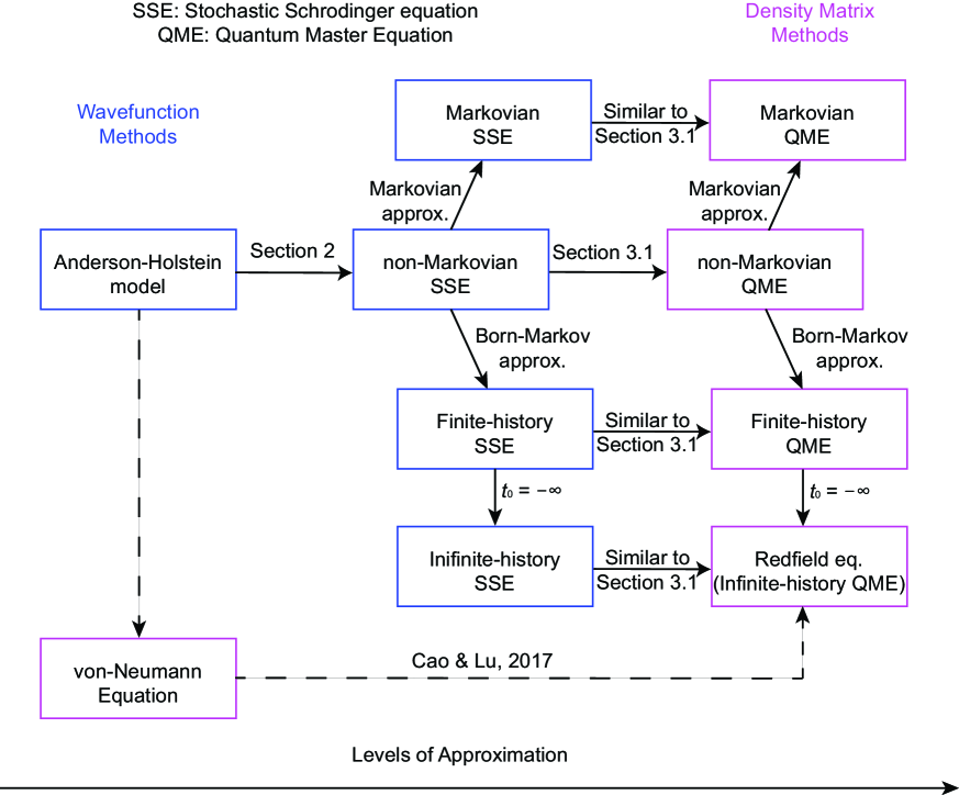
Refer to caption
Figure 1: Hierarchy of various models for Anderson-Holstein impurities.

Going from SSE, to QME, and further to classical master equations (CME), one will make more assumptions and conduct more approximations. As a result, one would possibly lose crucial physical features while going along this hierarchy of approximations.

IV Numerical Methods

IV.1 Noise Generation

To numerically simulate SSE, we need to generate stochastic noises that are subject to Eq. 38. The conventional noise generation scheme [47] relies on the analytic continuation of the correlation function to the complex plane. Such methods suffer from non-causality and non-physical artifacts due to the numerical instability of many rational approximation schemes [50, 51]. Here we present a stable noise generation scheme which do not rely on the interpolation of any correlation function.

We first rewrite the noise term as follows:

\displaystyle- iλV(x)2(ξ2(t)σx+ξ1(t)σy)(ψ0(x,t)ψ1(x,t))i𝜆𝑉𝑥2subscript𝜉2𝑡subscript𝜎𝑥subscript𝜉1𝑡subscript𝜎𝑦subscript𝜓0𝑥𝑡subscript𝜓1𝑥𝑡\displaystyle\frac{\mathrm{i}\lambda V(x)}{2}\left(\xi_{2}(t)\sigma_{x}+\xi_{1}(t)\sigma_{y}\right)\left(\begin{array}[]{l}\psi_{0}(x,t)\\ \psi_{1}(x,t)\end{array}\right) (55)
=\displaystyle= λV(x)(ξ~+(t)ψ1(x,t)ξ~(t)ψ0(x,t)),𝜆𝑉𝑥subscript~𝜉𝑡subscript𝜓1𝑥𝑡subscript~𝜉𝑡subscript𝜓0𝑥𝑡\displaystyle\lambda V(x)\left(\begin{array}[]{l}\widetilde{\xi}_{+}(t)\psi_{1}(x,t)\\ \widetilde{\xi}_{-}(t)\psi_{0}(x,t)\end{array}\right),
ξ~+(t)=subscript~𝜉𝑡absent\displaystyle\widetilde{\xi}_{+}(t)= ξ1(t)iξ2(t)2,ξ~(t)=ξ1(t)iξ2(t)2.subscript𝜉1𝑡isubscript𝜉2𝑡2subscript~𝜉𝑡subscript𝜉1𝑡isubscript𝜉2𝑡2\displaystyle\frac{-\xi_{1}(t)-\mathrm{i}\xi_{2}(t)}{2},\quad\widetilde{\xi}_{-}(t)=\frac{\xi_{1}(t)-\mathrm{i}\xi_{2}(t)}{2}.

where ξ~±(t)subscript~𝜉plus-or-minus𝑡\tilde{\xi}_{\pm}(t) satisfies that,

𝔼(ξ~±(t))=0,𝔼subscript~𝜉plus-or-minus𝑡0\displaystyle\mathbb{E}(\widetilde{\xi}_{\pm}(t))=0, 𝔼(ξ~+(t)ξ~(t))=0,𝔼superscriptsubscript~𝜉𝑡subscript~𝜉superscript𝑡0\displaystyle\quad\mathbb{E}(\widetilde{\xi}_{+}^{*}(t)\widetilde{\xi}_{-}(t^{\prime}))=0, (56)
𝔼(ξ~±(t)ξ~±(t))𝔼subscript~𝜉plus-or-minus𝑡subscript~𝜉plus-or-minussuperscript𝑡\displaystyle\mathbb{E}(\widetilde{\xi}_{\pm}(t)\widetilde{\xi}_{\pm}(t^{\prime})) =𝔼(ξ~±(t)ξ~(t))=0,absent𝔼subscript~𝜉plus-or-minus𝑡subscript~𝜉minus-or-plussuperscript𝑡0\displaystyle=\mathbb{E}(\widetilde{\xi}_{\pm}(t)\widetilde{\xi}_{\mp}(t^{\prime}))=0,\quad
𝔼(ξ~+(t)ξ~+(t))𝔼superscriptsubscript~𝜉𝑡subscript~𝜉superscript𝑡\displaystyle\mathbb{E}(\widetilde{\xi}_{+}^{*}(t)\widetilde{\xi}_{+}(t^{\prime})) =c+(tt),absentsuperscript𝑐𝑡superscript𝑡\displaystyle=c^{+}(t-t^{\prime}),
𝔼(ξ~(t)ξ~(t))𝔼superscriptsubscript~𝜉𝑡subscript~𝜉superscript𝑡\displaystyle\mathbb{E}(\widetilde{\xi}_{-}^{*}(t)\widetilde{\xi}_{-}(t^{\prime})) =c(tt).absentsuperscript𝑐𝑡superscript𝑡\displaystyle=c^{-}(t-t^{\prime}).

In this way, ξ~+(t)subscript~𝜉𝑡\tilde{\xi}_{+}(t) and ξ~(t)subscript~𝜉𝑡\tilde{\xi}_{-}(t) are decoupled, and could be generated separately. Let us define

W±(t)=0tξ~±(τ)dτ,subscript𝑊plus-or-minus𝑡superscriptsubscript0𝑡subscript~𝜉plus-or-minus𝜏differential-d𝜏W_{\pm}(t)=\int_{0}^{t}\tilde{\xi}_{\pm}(\tau)\mathrm{d}\tau,

Then W±(t)subscript𝑊plus-or-minus𝑡W_{\pm}(t) is a Gaussian process with the covariance function K(t,s)𝐾𝑡𝑠K(t,s):

K±(s,t)=0sdτ10tdτ2c±(τ1τ2).subscript𝐾plus-or-minus𝑠𝑡subscriptsuperscript𝑠0differential-dsubscript𝜏1subscriptsuperscript𝑡0differential-dsubscript𝜏2superscript𝑐plus-or-minussubscript𝜏1subscript𝜏2K_{\pm}(s,t)=\int^{s}_{0}\mathrm{d}\tau_{1}\int^{t}_{0}\mathrm{d}\tau_{2}c^{\pm}(\tau_{1}-\tau_{2}).

In particular, when c±(τ1τ2)=δ(τ1τ2)superscript𝑐plus-or-minussubscript𝜏1subscript𝜏2𝛿subscript𝜏1subscript𝜏2c^{\pm}(\tau_{1}-\tau_{2})=\delta(\tau_{1}-\tau_{2}), we have K±(s,t)=min(s,t)subscript𝐾plus-or-minus𝑠𝑡𝑠𝑡K_{\pm}(s,t)=\min(s,t), and W±(t)subscript𝑊plus-or-minus𝑡W_{\pm}(t) is the standard Brownian motion.

Generally, the sampling of W±(t)subscript𝑊plus-or-minus𝑡W_{\pm}(t) can be achieved by the Karhunen-Loève expansion. For a specified maximum time Tmaxsubscript𝑇maxT_{\text{max}}, consider the following eigenvalue problem:

0TmaxK±(s,t)ϕi±(t)dt=λi±ϕi±(s),i=1,2,formulae-sequencesuperscriptsubscript0subscript𝑇maxsubscript𝐾plus-or-minus𝑠𝑡subscriptsuperscriptitalic-ϕplus-or-minus𝑖𝑡differential-d𝑡subscriptsuperscript𝜆plus-or-minus𝑖subscriptsuperscriptitalic-ϕplus-or-minus𝑖𝑠𝑖12\int_{0}^{T_{\text{max}}}K_{\pm}(s,t)\phi^{\pm}_{i}(t)\mathrm{d}t=\lambda^{\pm}_{i}\phi^{\pm}_{i}(s),\quad i=1,2,\ldots (57)

with the normalization condition 0Tmaxϕi±ϕj±dt=δijsuperscriptsubscript0subscript𝑇maxsuperscriptsubscriptitalic-ϕ𝑖plus-or-minussuperscriptsubscriptitalic-ϕ𝑗plus-or-minusdifferential-d𝑡subscript𝛿𝑖𝑗\int_{0}^{T_{\text{max}}}\phi_{i}^{\pm}\phi_{j}^{\pm}\mathrm{d}t=\delta_{ij}. Then W±(t)subscript𝑊plus-or-minus𝑡W_{\pm}(t) has the Karhunen-Loève expansion

W±(t)=k=1αk±λk±ϕk±(t)subscript𝑊plus-or-minus𝑡superscriptsubscript𝑘1superscriptsubscript𝛼𝑘plus-or-minussuperscriptsubscript𝜆𝑘plus-or-minussuperscriptsubscriptitalic-ϕ𝑘plus-or-minus𝑡W_{\pm}(t)=\sum_{k=1}^{\infty}\alpha_{k}^{\pm}\sqrt{\lambda_{k}^{\pm}}\phi_{k}^{\pm}(t) (58)

Here the αkN(0,1)similar-tosubscript𝛼𝑘𝑁01\alpha_{k}\sim N(0,1) are i.i.d. random variables. In this way, the task of sampling the time-dependent noise is reduced to sampling scalar time-independent random variables. The eigenvalue problem Eq. 57 could be solved with a finite difference discretization in the time variable.

IV.2 Time evolution

We are solving Eq. 41 on the spatial domain [a,b]𝑎𝑏[a,b] and for time [0,T]0𝑇[0,T]. We use the following discretization:

Δx=(ba)M,Δ𝑥𝑏𝑎𝑀\displaystyle\Delta x=\dfrac{(b-a)}{M}, Δt=TN.Δ𝑡𝑇𝑁\displaystyle\Delta t=\dfrac{T}{N}. (59)
xj:=a+jΔx,assignsubscript𝑥𝑗𝑎𝑗Δ𝑥\displaystyle x_{j}:=a+j\Delta x, j=0,1,,M1,𝑗01𝑀1\displaystyle j=0,1,\cdots,M-1,
tn:=nΔt,assignsubscript𝑡𝑛𝑛Δ𝑡\displaystyle t_{n}:=n\Delta t, n=0,1,2,N.𝑛012𝑁\displaystyle n=0,1,2\cdots,N.

To numerically solve Eq. 41, our strategy is as follows:

  • For the system Hamiltonian H^Ssubscript^𝐻𝑆\hat{H}_{S}, we use the Time Splitting Spectral method [52];

  • For the fluctuation and dissipation terms, we use the Euler-Maruyama algorithm [53].

Let us present the numerical algorithm in detail for the Markovian SSE. With an efficient evaluation of the integration term, the strategy we described below is applicable to the non-Markovian case. In the Markovian limit, let c±(t)subscript𝑐plus-or-minus𝑡c_{\pm}(t) becomes c0±δ(t)superscriptsubscript𝑐0plus-or-minus𝛿𝑡c_{0}^{\pm}\delta(t), where c0±superscriptsubscript𝑐0plus-or-minusc_{0}^{\pm} are fixed constant. Then Eq. 41 becomes

iε(dψ0(x,t)dψ1(x,t))i𝜀dsubscript𝜓0𝑥𝑡dsubscript𝜓1𝑥𝑡\displaystyle\mathrm{i}\varepsilon\left(\begin{array}[]{c}\mathrm{d}\psi_{0}(x,t)\\ \mathrm{d}\psi_{1}(x,t)\end{array}\right) (60)
=\displaystyle= (h^0ψ0(x,t)h^1ψ1(x,t))dt+λV(x)(ψ1(x,t)dW1(t)ψ0(x,t)dW0(t))subscript^0subscript𝜓0𝑥𝑡subscript^1subscript𝜓1𝑥𝑡d𝑡𝜆𝑉𝑥subscript𝜓1𝑥𝑡dsubscript𝑊1𝑡subscript𝜓0𝑥𝑡dsubscript𝑊0𝑡\displaystyle\left(\begin{array}[]{c}\hat{h}_{0}\psi_{0}(x,t)\\ \hat{h}_{1}\psi_{1}(x,t)\end{array}\right)\mathrm{d}t+\lambda V(x)\left(\begin{array}[]{l}\psi_{1}(x,t)\mathrm{d}W_{1}(t)\\ \psi_{0}(x,t)\mathrm{d}W_{0}(t)\end{array}\right)
+iλ2ε|V(x)|2(c0ψ0(x,t)c0+ψ1(x,t))dt,x[a,b],isuperscript𝜆2𝜀superscript𝑉𝑥2superscriptsubscript𝑐0subscript𝜓0𝑥𝑡superscriptsubscript𝑐0subscript𝜓1𝑥𝑡d𝑡𝑥𝑎𝑏\displaystyle+\frac{\mathrm{i}\lambda^{2}}{\varepsilon}|V(x)|^{2}\left(\begin{array}[]{c}c_{0}^{-}\psi_{0}(x,t)\\ c_{0}^{+}\psi_{1}(x,t)\end{array}\right)\mathrm{d}t,\quad x\in[a,b],

Let us consider the following initial condition, which means that at t=0𝑡0t=0 the molecule is neutral:

(ψ0(x,0)ψ1(x,0))=(ψ0(x,0)0).subscript𝜓0𝑥0subscript𝜓1𝑥0subscript𝜓0𝑥00\left(\begin{array}[]{c}\psi_{0}(x,0)\\ \psi_{1}(x,0)\end{array}\right)=\left(\begin{array}[]{c}\psi_{0}(x,0)\\ 0\end{array}\right).

Denote the numerical solution of ψk(xj,tn),k=0,1formulae-sequencesubscript𝜓𝑘subscript𝑥𝑗subscript𝑡𝑛𝑘01\psi_{k}(x_{j},t_{n}),k=0,1 by ψkj,n,k=0,1formulae-sequencesuperscriptsubscript𝜓𝑘𝑗𝑛𝑘01\psi_{k}^{j,n},k=0,1. From time t=tn𝑡subscript𝑡𝑛t=t_{n} to time t=tn+1𝑡subscript𝑡𝑛1t=t_{n+1}, we do the following:

  1. 1.

    Evolve using the potential term for a time step:

    ψkj,1=exp(iUk(xj)εΔt)ψkj,n,superscriptsubscript𝜓𝑘𝑗absent1isubscript𝑈𝑘subscript𝑥𝑗𝜀Δ𝑡superscriptsubscript𝜓𝑘𝑗𝑛\displaystyle\psi_{k}^{j,*1}=\exp{\left(-\mathrm{i}\frac{U_{k}(x_{j})}{\varepsilon}\Delta t\right)}\psi_{k}^{j,n}, (61)
    k=0,1,j=0,,M1,formulae-sequence𝑘01𝑗0𝑀1\displaystyle k=0,1,\quad j=0,\cdots,M-1,
  2. 2.

    Evolve using the kinetic term for a time step, but in the frequency domain: for k=0,1𝑘01k=0,1, we have

    {{ψ^kl,1}l=M2M21=FFT({ψkj,1}j=0M1),ψ^kl,2=ψ^kl,1exp(iεμl22Δt), l=M2,,M21,{ψkj,2}j=0M1=iFFT({ψ^kl,2}l=M2M21).casessuperscriptsubscriptsuperscriptsubscript^𝜓𝑘𝑙absent1𝑙𝑀2𝑀21FFTsuperscriptsubscriptsuperscriptsubscript𝜓𝑘𝑗absent1𝑗0𝑀1otherwiseformulae-sequencesuperscriptsubscript^𝜓𝑘𝑙absent2superscriptsubscript^𝜓𝑘𝑙absent1i𝜀superscriptsubscript𝜇𝑙22Δ𝑡 𝑙𝑀2𝑀21otherwisesuperscriptsubscriptsuperscriptsubscript𝜓𝑘𝑗absent2𝑗0𝑀1iFFTsuperscriptsubscriptsuperscriptsubscript^𝜓𝑘𝑙absent2𝑙𝑀2𝑀21otherwise\displaystyle\begin{cases}\{\widehat{\psi}_{k}^{l,*1}\}_{l=-\frac{M}{2}}^{\frac{M}{2}-1}=\mbox{FFT}\left(\{\psi_{k}^{j,*1}\}_{j=0}^{M-1}\right),\\ \widehat{\psi}_{k}^{l,*2}=\widehat{\psi}_{k}^{l,*1}\exp{\left(-\mathrm{i}\varepsilon\frac{\mu_{l}^{2}}{2}\Delta t\right)},\text{ }l=-\frac{M}{2},\cdots,\frac{M}{2}-1,\\ \{\psi_{k}^{j,*2}\}_{j=0}^{M-1}=\mbox{iFFT}\left(\{\widehat{\psi}_{k}^{l,*2}\}_{l=-\frac{M}{2}}^{\frac{M}{2}-1}\right).\end{cases} (62)

    Here μl=2πlbasubscript𝜇𝑙2𝜋𝑙𝑏𝑎\mu_{l}=\dfrac{2\pi l}{b-a}, FFT and iFFT denote the Fast Fourier Transform and its inverse.

  3. 3.

    Deal with the fluctuation-dissipation term using the Euler-Maruyama scheme:

    (ψ0j,n+1ψ1j,n+1)superscriptsubscript𝜓0𝑗𝑛1superscriptsubscript𝜓1𝑗𝑛1\displaystyle\left(\begin{array}[]{l}\psi_{0}^{j,n+1}\\ \psi_{1}^{j,n+1}\end{array}\right) (63)
    =(ψ0j,2ψ1j,2)iλV(xj)ε((W1(tn+1)W1(tn))ψ1j,2(W0(tn+1)W0(tn))ψ0j,2)absentsuperscriptsubscript𝜓0𝑗absent2superscriptsubscript𝜓1𝑗absent2i𝜆𝑉subscript𝑥𝑗𝜀subscript𝑊1subscript𝑡𝑛1subscript𝑊1subscript𝑡𝑛superscriptsubscript𝜓1𝑗absent2subscript𝑊0subscript𝑡𝑛1subscript𝑊0subscript𝑡𝑛superscriptsubscript𝜓0𝑗absent2\displaystyle=\left(\begin{array}[]{l}\psi_{0}^{j,*2}\\ \psi_{1}^{j,*2}\end{array}\right)-\mathrm{i}\dfrac{\lambda V(x_{j})}{\varepsilon}\left(\begin{array}[]{l}\left(W_{1}(t_{n+1})-W_{1}(t_{n})\right)\psi_{1}^{j,*2}\\ \left(W_{0}(t_{n+1})-W_{0}(t_{n})\right)\psi_{0}^{j,*2}\end{array}\right)
    +λ2ε2|V(xj)|2(c0ψ0j,2c0+ψ1j,2)Δt.superscript𝜆2superscript𝜀2superscript𝑉subscript𝑥𝑗2superscriptsubscript𝑐0superscriptsubscript𝜓0𝑗absent2superscriptsubscript𝑐0superscriptsubscript𝜓1𝑗absent2Δ𝑡\displaystyle+\dfrac{\lambda^{2}}{\varepsilon^{2}}|V(x_{j})|^{2}\left(\begin{array}[]{l}c_{0}^{-}\psi_{0}^{j,*2}\\ c_{0}^{+}\psi_{1}^{j,*2}\end{array}\right)\Delta t.
Remark 1.

Here we use a first-order splitting scheme for the Hamiltonian part, which is sufficient for our problem. Higher-order splitting schemes also exist, such as Strang-Splitting and so on.

V Numerical Results

The purpose of our numerical experiments is two-fold. On the one hand, we demonstrate that an ensemble of realizations of SSE could be used to obtain samples of physical observables of interest and thus directly manifest distributional information of these quantities, while QME could not provide a detailed characterization of the distribution except for moment information. On the other hand, we show that SSE and QME approaches indeed have the same thermodynamic equilibrium, while exhibiting different transient dynamics towards reaching such equilibrium.

V.1 Samples of physical observables by SSE

Let x[a,b]=[π,π]𝑥𝑎𝑏𝜋𝜋x\in[a,b]=[-\pi,\pi], the maximal time T=10𝑇10T=10. For simplicity, in this subsection, we choose the interaction strength λ=ε𝜆𝜀\lambda=\varepsilon, which is neither necessary nor essential. Let us focus on the following system potentials which are harmonic with different centers:

U0(x)=12x2,U1(x)=12x2+0.1x.formulae-sequencesubscript𝑈0𝑥12superscript𝑥2subscript𝑈1𝑥12superscript𝑥20.1𝑥U_{0}(x)=\frac{1}{2}x^{2},\quad U_{1}(x)=\frac{1}{2}x^{2}+0.1x.

We aim to numerically explore SSE (60) in the wide band limit and with δ𝛿\delta-correlated noise with special attention to investigating the role of the coupling potential V(x)𝑉𝑥V(x). To this end, we consider the following examples:

Example 1. Propagating a Gaussian wavepacket with a bimodal coupling function:

ψ0(x,0)subscript𝜓0𝑥0\displaystyle\psi_{0}(x,0) =1(πε)14exp((xq0)22ε+ip0(xq0)ε),absent1superscript𝜋𝜀14superscript𝑥subscript𝑞022𝜀isubscript𝑝0𝑥subscript𝑞0𝜀\displaystyle=\dfrac{1}{(\pi\varepsilon)^{\frac{1}{4}}}\exp{\left(\frac{-(x-q_{0})^{2}}{2\varepsilon}+\mathrm{i}\frac{p_{0}(x-q_{0})}{\varepsilon}\right)}, (64)
V(x)𝑉𝑥\displaystyle V(x) =exp(10(x0.5)2)+exp(40(x+2)21),absent10superscript𝑥0.5240superscript𝑥221\displaystyle=\exp{\left(-10(x-0.5)^{2}\right)}+\exp{\left(-40(x+2)^{2}-1\right)},
q0subscript𝑞0\displaystyle q_{0} =1,p0=0.5,formulae-sequenceabsent1subscript𝑝00.5\displaystyle=-1,p_{0}=0.5,

Example 2. Propagating a Gaussian wavepacket with another bimodal coupling function:

ψ0(x)subscript𝜓0𝑥\displaystyle\psi_{0}(x) =1(πε)14exp((xq0)22ε+ip0(xq0)ε),absent1superscript𝜋𝜀14superscript𝑥subscript𝑞022𝜀isubscript𝑝0𝑥subscript𝑞0𝜀\displaystyle=\dfrac{1}{(\pi\varepsilon)^{\frac{1}{4}}}\exp{\left(\frac{-(x-q_{0})^{2}}{2\varepsilon}+\mathrm{i}\frac{p_{0}(x-q_{0})}{\varepsilon}\right)}, (65)
V(x)𝑉𝑥\displaystyle V(x) =2exp(10(x0.9)2)+5exp(40(x+0.5)2),absent210superscript𝑥0.92540superscript𝑥0.52\displaystyle=2\exp{\left(-10(x-0.9)^{2}\right)}+5\exp{\left(-40(x+0.5)^{2}\right)},
q0subscript𝑞0\displaystyle q_{0} =1,p0=0.5.formulae-sequenceabsent1subscript𝑝00.5\displaystyle=-1,p_{0}=0.5.

Example 3. Propagating a non-Gaussian wavepacket with a unimodal coupling function:

ψ0(x)subscript𝜓0𝑥\displaystyle\psi_{0}(x) exp(5(x+1)2+isin(x)ε),proportional-toabsent5superscript𝑥12i𝑥𝜀\displaystyle\propto\exp{\left(-5(x+1)^{2}+\mathrm{i}\frac{\sin(x)}{\varepsilon}\right)}, (66)
V(x)𝑉𝑥\displaystyle V(x) =exp(10x2).absent10superscript𝑥2\displaystyle=\exp{\left(-10x^{2}\right)}.

The coupling functions V(x)𝑉𝑥V(x) that we considered are shown in Fig. 2. We remark that the experiments are designed such that either the wave packet is expected to exhibit decoherence through the interaction with the bath or is not initialized from a coherent state.
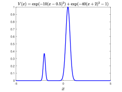
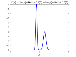
Refer to caption
Refer to caption
Refer to caption
Figure 2: Plots of coupling functions V(x)𝑉𝑥V(x) in example 1, 2 and 3.

A typical trajectory of time evolution of SSE is shown in Fig. 3. We observe that the wave function is initially populated solely on level-0, it oscillates and propagates within a finite region due to the confinement of the harmonic potentials. In particular, only when it passes through an interaction region (where the coupling potential V(x)𝑉𝑥V(x) is significant), it will partially and stochastically transmit to the other level. Thus the resulting dynamical behavior is rather complicated and the nonadiabatic phenomenon is nontrivial.
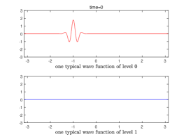
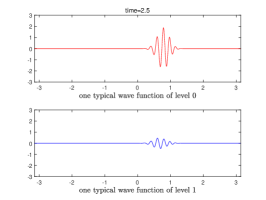
Refer to caption
Refer to caption
Refer to caption
Refer to caption
Refer to caption
Figure 3: The evolution of a typical wavefunction trajectory in example 111.

To explore the stochasticity of the SSE model, let us demonstrate with the numerical simulations of certain physical observables computed via an ensemble of realizations of SSE (60). We consider the transition rate R(t)delimited-⟨⟩𝑅𝑡\langle R(t)\rangle and spatial average X(t)delimited-⟨⟩𝑋𝑡\langle X(t)\rangle, defined as:

R(t)=|ψ0(x,t)|2dx(|ψ0(x,t)|2+|ψ1(x,t)|2)dx,delimited-⟨⟩𝑅𝑡superscriptsubscript𝜓0𝑥𝑡2differential-d𝑥superscriptsubscript𝜓0𝑥𝑡2superscriptsubscript𝜓1𝑥𝑡2differential-d𝑥\displaystyle\langle R(t)\rangle=\frac{\int|\psi_{0}(x,t)|^{2}\mathrm{d}x}{\int\left(|\psi_{0}(x,t)|^{2}+|\psi_{1}(x,t)|^{2}\right)\mathrm{d}x}, (67)
X(t)=x(|ψ0(x,t)|2+|ψ1(x,t)|2)dx(|ψ0(x,t)|2+|ψ1(x,t)|2)dx,delimited-⟨⟩𝑋𝑡𝑥superscriptsubscript𝜓0𝑥𝑡2superscriptsubscript𝜓1𝑥𝑡2differential-d𝑥superscriptsubscript𝜓0𝑥𝑡2superscriptsubscript𝜓1𝑥𝑡2differential-d𝑥\displaystyle\langle X(t)\rangle=\frac{\int x\left(|\psi_{0}(x,t)|^{2}+|\psi_{1}(x,t)|^{2}\right)\mathrm{d}x}{\int\left(|\psi_{0}(x,t)|^{2}+|\psi_{1}(x,t)|^{2}\right)\mathrm{d}x},

We emphasize that delimited-⟨⟩\langle\cdot\rangle mean taking the average over the quantum state, which is obtained by a one-time realization of SSE (60). Hence, R(t)delimited-⟨⟩𝑅𝑡\langle R(t)\rangle and X(t)delimited-⟨⟩𝑋𝑡\langle X(t)\rangle are random variables due to the stochasticity in the dynamics of (60). We repeat simulation (60) of each exmaple for 400040004000 times, and the statistics (in the form of the histogram) of the observables are shown in Fig. 4, Fig. 5 and Fig. 6, respectively.
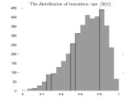
Refer to caption
Refer to caption
Refer to caption
Refer to caption
Figure 4: Histogram for transition rate and atomic position at T=10𝑇10T=10, with ε=1/32𝜀132\varepsilon=1/32 and ε=1/64𝜀164\varepsilon=1/64, in example 1, from 4000 trajectories. The two subfigures on the left correspond to λ=1/32𝜆132\lambda=1/32 and the ones on the right correspond to λ=1/64𝜆164\lambda=1/64. This demonstrates a transition rate with a non-Gaussian distribution but an atomic position with a Gaussian-like distribution.
Refer to caption
Refer to caption
Figure 5: Histogram for transition rate and atomic position at T=10𝑇10T=10, with ε=1/32𝜀132\varepsilon=1/32, in example 2, from 4000 trajectories. This demonstrates a transition rate with a Gaussian-like distribution but an atomic position with a non-Gaussian distribution.
Refer to caption
Refer to caption
Refer to caption
Refer to caption
Figure 6: Histogram for transition rate and atomic position at T=10𝑇10T=10, with ε=1/32𝜀132\varepsilon=1/32 and ε=1/64𝜀164\varepsilon=1/64, in example 3, from 4000 trajectories. The two subfigures on the left correspond to λ=1/32𝜆132\lambda=1/32 and the ones on the right correspond to λ=1/64𝜆164\lambda=1/64. This shows that the transition rate and atomic position both have a Gaussian-like distribution.

We can see that the coupling function V(x)𝑉𝑥V(x) significantly affects the probability distribution of physical observables and SSE is capable of capturing both Gaussian and non-Gaussian distributional information of these quantities. Specifically, we have the following observations:

  • (1)

    In Example 1, the coupling function V(x)𝑉𝑥V(x) is bimodal: the primary coupling peak is placed near the center of the propagation region and the secondary coupling peak is placed near the boundary of the propagation region, where wave function turns its moving direction. We observe that the distribution of transition rate R(t)delimited-⟨⟩𝑅𝑡\langle R(t)\rangle is non-Gaussian but the distribution of atomic position X(t)delimited-⟨⟩𝑋𝑡\langle X(t)\rangle is Gaussian;

  • (2)

    In Example 2, the coupling function V(x)𝑉𝑥V(x) is also bimodal: both coupling peaks are near the center of the propagation region, but they are of different profiles. We observe that the distribution of transition rate R(t)delimited-⟨⟩𝑅𝑡\langle R(t)\rangle is Gaussian but the distribution of atomic position X(t)delimited-⟨⟩𝑋𝑡\langle X(t)\rangle is non-Gaussian;

  • (3)

    In Example 3, although the wave function is initialized far from a coherent state, the coupling function V(x)𝑉𝑥V(x) is unimodal, we have the distributions of transition rate R(t)delimited-⟨⟩𝑅𝑡\langle R(t)\rangle and atomic position X(t)delimited-⟨⟩𝑋𝑡\langle X(t)\rangle are both Gaussian.

While the results above are not conclusively definitive, this set of experiments already sheds light on the diverse stochastic behavior contained within the SSE models.

V.2 Comparison between SSE and QME

This part is devoted to a detailed comparison between SSE and QME models both in dynamics and equilibrium. Consider [44, 14, 48]

U0(x)subscript𝑈0𝑥\displaystyle U_{0}(x) =12x2,U1(x)=U0(x)+2gx+g2+Ed,formulae-sequenceabsent12superscript𝑥2subscript𝑈1𝑥subscript𝑈0𝑥2𝑔𝑥superscript𝑔2subscript𝐸𝑑\displaystyle=\frac{1}{2}x^{2},\quad U_{1}(x)=U_{0}(x)+\sqrt{2}gx+g^{2}+E_{d}, (68)

with the Markovian assumption c±(τ)=c0±δ(τ)superscript𝑐plus-or-minus𝜏superscriptsubscript𝑐0plus-or-minus𝛿𝜏c^{\pm}(\tau)=c_{0}^{\pm}\delta(\tau), the corresponding QME of Eq. 49, transformed back to the Schrödinger picture, is

dρ(t)dt=iε[H^S,ρ(t)]d𝜌𝑡d𝑡i𝜀subscript^𝐻𝑆𝜌𝑡\displaystyle\frac{\mathrm{d}\rho(t)}{\mathrm{d}t}=-\frac{\mathrm{i}}{\varepsilon}\left[\hat{H}_{S},\rho(t)\right] (69)
+\displaystyle+ λ2ε2|V|2(2(ρ00(t)ρ11(t))ρ01(t)+ρ10(t)ρ01(t)+ρ10(t)2(ρ11(t)ρ00(t))).superscript𝜆2superscript𝜀2superscript𝑉2matrix2subscript𝜌00𝑡subscript𝜌11𝑡subscript𝜌01𝑡subscript𝜌10𝑡subscript𝜌01𝑡subscript𝜌10𝑡2subscript𝜌11𝑡subscript𝜌00𝑡\displaystyle\frac{\lambda^{2}}{\varepsilon^{2}}|V|^{2}\begin{pmatrix}2(\rho_{00}(t)-\rho_{11}(t))&\rho_{01}(t)+\rho_{10}(t)\\ \rho_{01}(t)+\rho_{10}(t)&2(\rho_{11}(t)-\rho_{00}(t))\end{pmatrix}.

This is equivalent to the traditional Markovian QME

iεdρ(t)dt=[(h^000h^1),ρ(t)]i𝜀d𝜌𝑡d𝑡matrixsubscript^000subscript^1𝜌𝑡\displaystyle\mathrm{i}\varepsilon\frac{\mathrm{d}\rho(t)}{\mathrm{d}t}=\left[\begin{pmatrix}\hat{h}_{0}&0\\ 0&\hat{h}_{1}\end{pmatrix},\rho(t)\right] (70)
\displaystyle- iλ2V2ε[d^d^ρ(t)d^ρ(t)d^+ρ(t)d^d^d^ρ(t)d^+h.c.],\displaystyle\mathrm{i}\frac{\lambda^{2}V^{2}}{\varepsilon}\left[\hat{d}\hat{d}^{\dagger}\rho(t)-\hat{d}^{\dagger}\rho(t)\hat{d}+\rho(t)\hat{d}^{\dagger}\hat{d}-\hat{d}\rho(t)\hat{d}^{\dagger}+h.c.\right],

where d^^𝑑\hat{d} and d^superscript^𝑑\hat{d}^{\dagger} are defined as in (4). We choose the following parameter:

L=20,g=0.1,Ed=0.1,V(x)=1,formulae-sequence𝐿20formulae-sequence𝑔0.1formulae-sequencesubscript𝐸𝑑0.1𝑉𝑥1\displaystyle L=20,\quad g=0.1,\quad E_{d}=0.1,\quad V(x)=1, (71)

and the initial value

ψ0(x,0)1,ρ(x,x,0)=ψ0(x,0)ψ0(x,0).formulae-sequenceproportional-tosubscript𝜓0𝑥01𝜌𝑥superscript𝑥0subscript𝜓0𝑥0subscriptsuperscript𝜓0superscript𝑥0\psi_{0}(x,0)\propto 1,\quad\rho(x,x^{\prime},0)=\psi_{0}(x,0)\psi^{*}_{0}(x^{\prime},0).

In this example, we conduct the spatial discretization with Hermite polynomials. Also, note that the coupling function V𝑉V is chosen to be spatially homogeneous, and the system is expected to reach the equilibrium.

Recall that the proposed models in this work are characterized by two parameters: the interaction strength λ𝜆\lambda and the semiclassical parameter ε𝜀\varepsilon. From the derivation of QME based on SSE, we can see that it holds when λ1much-less-than𝜆1\lambda\ll 1 while ε𝜀\varepsilon is fixed, and a recent mathematical study reveals that QME can be directly derived only if λεmuch-less-than𝜆𝜀\lambda\ll\varepsilon [44]. In fact, our formulation facilitates more systematic comparisons between SSE and QME with various combinations of λ𝜆\lambda and ε𝜀\varepsilon. The purpose of the following two numerical experiments is to compare the dynamics and steady states between SSE and QME under different ε𝜀\varepsilon versus λ𝜆\lambda relationships.

In the two numerical experiments, we test with two different ε=1/32𝜀132\varepsilon=1/32 and 1/641641/64. For each ε𝜀\varepsilon, we let the λ𝜆\lambda vary from ε𝜀\varepsilon to ε/8𝜀8\varepsilon/8. The evolutions of the population of electrons on two levels based on SSE and QME for different ε𝜀\varepsilon and λ𝜆\lambda are shown in Fig. 7 and Fig. 8. The result indicates that (1) in this parameter setting, SSE and QME have the same equilibrium but different transient dynamics, and QME will reach the steady state faster than SSE; (2) for a fixed ε𝜀\varepsilon, λ𝜆\lambda only affects the relaxation time to reach the equilibrium, and a smaller λ𝜆\lambda indicates a longer relaxation time.

The former observation can be understood in two ways. Mathematically, the QME is not exactly equivalent to SSE, they are equal only if the higher-order term O(λ3)𝑂superscript𝜆3O(\lambda^{3}) is ignored. In a short time, the higher order terms lead to a difference in the dynamical behavior of the two, but in a long time, the higher order terms cancel each other out and thus have no effect on the steady state. Scientifically, QME is averaged over the stochastic term, such that the dissipation terms do not compete with the random fluctuations in dynamics, and thus the dynamics corresponding to QME will reach the steady state faster. This is a common relationship between SSE and QME and has been discussed in [54]. The latter shows that SSE still has the same steady state as QME when λ𝜆\lambda is not much less than ε𝜀\varepsilon, at least for a large class of parameter settings. This indicates that λεmuch-less-than𝜆𝜀\lambda\ll\varepsilon is only a sufficient condition, not a necessary one to establish qualitative connections between SSE and QME. More comparison studies and even qualitative connections are worth exploring in the future.
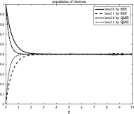
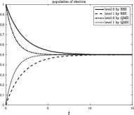
Refer to caption
Refer to caption
Refer to caption
Refer to caption
Figure 7: The population of electrons on two levels corresponding to ε=1/32𝜀132\varepsilon=1/32. From the top left to the bottom right, λ𝜆\lambda corresponds to ε,ε/2,ε/4𝜀𝜀2𝜀4\varepsilon,\varepsilon/2,\varepsilon/4, and ε/8𝜀8\varepsilon/8, respectively. The sample size of SSE is M=80000𝑀80000M=80000.
Refer to caption
Refer to caption
Refer to caption
Refer to caption
Figure 8: The population of electrons on two levels corresponding to ε=1/64𝜀164\varepsilon=1/64. From the top left to the bottom right, λ𝜆\lambda corresponds to ε,ε/2,ε/4𝜀𝜀2𝜀4\varepsilon,\varepsilon/2,\varepsilon/4, and ε/8𝜀8\varepsilon/8, respectively. The sample size of SSE is M=80000𝑀80000M=80000.

VI Conclusion and Discussions

In this article, we propose a stochastic Schrödinger equation model for the Anderson-Holstein impurities, filling a gap in the study of open quantum systems with fermionic baths. The SSE model is obtained directly from the microscopic model instead of using empirical correlation functions. Through analytic derivations, we establish the theoretical relations between AH, SSE and QME, and introduce the hierarchy of modeling in Fig. 1. We also discuss efficient algorithms for noise generation and sampling stochastic trajectories. Our numerical experiments show that SSE could be used to study physical observables and capture effects beyond the level of QME.

From the computational perspective, the non-Markovian term could be potentially expensive, especially in the high-dimensional case. If one is interested in the nonequilibrium dynamics of SSE, efficient algorithms that incorporate noise and treat the non-Markovian term with (quasi-)linear cost in time (for example, see [55]) would be required to propagate towards a longer time.

Our current studies focus on Holstein types of quantum impurities. Similar strategies are applicable to correlated systems via the pseudoparticle approach [56]. Understanding decoherence and relaxation dynamics of interacting systems [27, 57] will be the focus of our future work.

Acknowledgement

Z.Z. is supported by the National Key R&D Program of China, Project Number 2021YFA1001200, and the NSFC, grant Number 12031013, 12171013. This work is partially supported by a grant from the Simons Foundation under Award No. 825053 (Z.H.). We thank helpful discussions with Dr. Yu Cao. L.X. thanks Dr. Hao Wu for his support and encouragement.

All authors contribute equally to this work.

References

  • Anderson [1961] P. W. Anderson, Physical Review 124, 41 (1961).
  • Hanson et al. [2007] R. Hanson, L. P. Kouwenhoven, J. R. Petta, S. Tarucha, and L. M. Vandersypen, Reviews of modern physics 79, 1217 (2007).
  • Brako and Newns [1981] R. Brako and D. Newns, Journal of Physics C: Solid State Physics 14, 3065 (1981).
  • Newns [1969] D. Newns, Physical Review 178, 1123 (1969).
  • Holstein [1959] T. Holstein, Annals of physics 8, 325 (1959).
  • Persson [1993] B. Persson, The Journal of Chemical Physics 98, 1659 (1993).
  • Luo et al. [2016] X. Luo, B. Jiang, J. I. Juaristi, M. Alducin, and H. Guo, The Journal of Chemical Physics 145, 044704 (2016).
  • Nitzan and Ratner [2003] A. Nitzan and M. A. Ratner, Science 300, 1384 (2003).
  • Shenvi et al. [2009] N. Shenvi, S. Roy, and J. C. Tully, The Journal of chemical physics 130, 174107 (2009).
  • Huang et al. [2023a] Z. Huang, L. Xu, and Z. Zhou, Journal of Computational Physics 474, 111771 (2023a).
  • Katz et al. [2005] G. Katz, Y. Zeiri, and R. Kosloff, The Journal of Physical Chemistry B 109, 18876 (2005).
  • Shenvi et al. [2006] N. Shenvi, S. Roy, P. Parandekar, and J. Tully, The Journal of chemical physics 125 (2006).
  • Langreth and Nordlander [1991] D. C. Langreth and P. Nordlander, Physical Review B 43, 2541 (1991).
  • Dou and Subotnik [2016] W. Dou and J. E. Subotnik, The Journal of chemical physics 144, 024116 (2016).
  • Ouyang et al. [2015] W. Ouyang, J. G. Saven, and J. E. Subotnik, The Journal of Physical Chemistry C 119, 20833 (2015).
  • Miao et al. [2019] G. Miao, W. Ouyang, and J. Subotnik, The Journal of Chemical Physics 150 (2019).
  • Gao [1997] S. Gao, Physical review letters 79, 3101 (1997).
  • Wang et al. [2020] Y.-S. Wang, P. Nijjar, X. Zhou, D. I. Bondar, and O. V. Prezhdo, The Journal of Physical Chemistry B 124, 4326 (2020).
  • Nakajima [1958] S. Nakajima, Progress of Theoretical Physics 20, 948 (1958).
  • Fay [2021] T. P. Fay, The Journal of Physical Chemistry Letters 12, 1407 (2021).
  • Redfield [1965] A. G. Redfield, in Advances in Magnetic and Optical Resonance (Elsevier, 1965), vol. 1, pp. 1–32.
  • Leathers and Micha [2006] A. S. Leathers and D. A. Micha, The Journal of Physical Chemistry A 110, 749 (2006).
  • Elste et al. [2008] F. Elste, G. Weick, C. Timm, and F. von Oppen, Applied Physics A 93, 345 (2008).
  • Elste et al. [2010] F. Elste, D. R. Reichman, and A. J. Millis, Physical Review B 81, 205413 (2010).
  • Elste et al. [2011a] F. Elste, D. R. Reichman, and A. J. Millis, Physical Review B 83, 085415 (2011a).
  • Elste et al. [2011b] F. Elste, D. R. Reichman, and A. J. Millis, Physical Review B 83, 245405 (2011b).
  • Haertle et al. [2013] R. Haertle, G. Cohen, D. Reichman, and A. Millis, Physical Review B 88, 235426 (2013).
  • Tanimura and Kubo [1989] Y. Tanimura and R. Kubo, Journal of the Physical Society of Japan 58, 101 (1989).
  • Erpenbeck and Thoss [2019] A. Erpenbeck and M. Thoss, The Journal of Chemical Physics 151 (2019).
  • Goetsch et al. [1996] P. Goetsch, P. Tombesi, and D. Vitali, Physical Review A 54, 4519 (1996).
  • Shiokawa and Hu [1995] K. Shiokawa and B. Hu, Physical Review E 52, 2497 (1995).
  • Wiseman [1996] H. M. Wiseman, Quantum and Semiclassical Optics: Journal of the European Optical Society Part B 8, 205 (1996).
  • Gambetta and Wiseman [2002] J. Gambetta and H. M. Wiseman, Physical Review A 66, 012108 (2002).
  • Gambetta and Wiseman [2003] J. Gambetta and H. Wiseman, Physical Review A 68, 062104 (2003).
  • Breuer and Petruccione [1995] H.-P. Breuer and F. Petruccione, Physical Review E 52, 428 (1995).
  • Breuer and Piilo [2009] H.-P. Breuer and J. Piilo, Europhysics Letters 85, 50004 (2009).
  • Zhao et al. [2012] X. Zhao, W. Shi, L.-A. Wu, and T. Yu, Physical Review A 86, 032116 (2012).
  • Nathan and Rudner [2020] F. Nathan and M. S. Rudner, Physical Review B 102, 115109 (2020).
  • Breuer et al. [2002] H.-P. Breuer, F. Petruccione, et al., The theory of open quantum systems (Oxford University Press on Demand, 2002).
  • Strunz and Yu [2004] W. T. Strunz and T. Yu, Physical Review A 69, 052115 (2004).
  • Jentzen and Kloeden [2011] A. Jentzen and P. E. Kloeden, Taylor approximations for stochastic partial differential equations (SIAM, 2011).
  • Zhang and Karniadakis [2017] Z. Zhang and G. Karniadakis, Numerical methods for stochastic partial differential equations with white noise, vol. 196 (Springer, 2017).
  • Shi et al. [2013] W. Shi, X. Zhao, and T. Yu, Physical Review A 87, 052127 (2013).
  • Cao and Lu [2017] Y. Cao and J. Lu, Journal of Mathematical Physics 58, 122105 (2017), ISSN 0022-2488, 1089-7658, URL http://aip.scitation.org/doi/10.1063/1.4993431.
  • Bogoliubov [1947] N. Bogoliubov, J. Phys 11, 23 (1947).
  • Bogoljubov et al. [1958] N. Bogoljubov, V. V. Tolmachov, and D. Širkov, Fortschritte der physik 6, 605 (1958).
  • Gaspard and Nagaoka [1999] P. Gaspard and M. Nagaoka, The Journal of chemical physics 111, 5676 (1999).
  • Dou et al. [2015] W. Dou, A. Nitzan, and J. E. Subotnik, The Journal of Chemical Physics 142, 084110 (2015), ISSN 0021-9606, 1089-7690, URL http://aip.scitation.org/doi/10.1063/1.4908034.
  • Dou et al. [2017] W. Dou, G. Miao, and J. E. Subotnik, Physical Review Letters 119, 046001 (2017).
  • Trefethen [2019] L. N. Trefethen, Approximation Theory and Approximation Practice, Extended Edition (SIAM, 2019).
  • Huang et al. [2023b] Z. Huang, E. Gull, and L. Lin, Physical Review B 107, 075151 (2023b).
  • Bao et al. [2002] W. Bao, S. Jin, and P. A. Markowich, Journal of Computational Physics 175, 487 (2002).
  • Kloeden et al. [1992] P. E. Kloeden, E. Platen, P. E. Kloeden, and E. Platen, Stochastic differential equations (Springer, 1992).
  • Biele and D’Agosta [2012] R. Biele and R. D’Agosta, Journal of Physics: Condensed Matter 24, 273201 (2012).
  • Kaye and UR Strand [2023] J. Kaye and H. UR Strand, Advances in Computational Mathematics 49, 63 (2023).
  • Eckstein and Werner [2010] M. Eckstein and P. Werner, Physical Review B 82, 115115 (2010).
  • Haertle and Millis [2014] R. Haertle and A. Millis, Physical Review B 90, 245426 (2014).

Appendix A Derivation of nMQME from nMSSE

We fill in the details of deriving the nMQME Eq. 49. Recall that from Eq. 47

ΨI(2)(x,t)=i(0tH^int,I(2)(t1)dt1)ΨI(x,0)0tdt10t1dt2H^int,I(1)(t1)Hint,I(1)(t2)ΨI(x,0).subscriptsuperscriptΨ2𝐼𝑥𝑡isuperscriptsubscript0𝑡superscriptsubscript^𝐻int𝐼2subscript𝑡1differential-dsubscript𝑡1subscriptΨ𝐼𝑥0superscriptsubscript0𝑡differential-dsubscript𝑡1superscriptsubscript0subscript𝑡1differential-dsubscript𝑡2subscriptsuperscript^𝐻1int𝐼subscript𝑡1subscriptsuperscript𝐻1int𝐼subscript𝑡2subscriptΨ𝐼𝑥0\Psi^{(2)}_{I}(x,t)=-\mathrm{i}\left(\int_{0}^{t}\hat{H}_{\mathrm{int},I}^{(2)}(t_{1})\mathrm{d}t_{1}\right)\Psi_{I}(x,0)-\int_{0}^{t}\mathrm{d}t_{1}\int_{0}^{t_{1}}\mathrm{d}t_{2}\hat{H}^{(1)}_{\mathrm{int},I}(t_{1})H^{(1)}_{\mathrm{int},I}(t_{2})\Psi_{I}(x,0).

Therefore

𝔼(ΨI(2)(x,t))=i(0tH^int,I(2)(t1)dt1)ΨI(x,0)0tdt10t1dt2𝔼(H^int,I(1)(t1)Hint,I(1)(t2))ΨI(x,0).𝔼subscriptsuperscriptΨ2𝐼𝑥𝑡isuperscriptsubscript0𝑡superscriptsubscript^𝐻int𝐼2subscript𝑡1differential-dsubscript𝑡1subscriptΨ𝐼𝑥0superscriptsubscript0𝑡differential-dsubscript𝑡1superscriptsubscript0subscript𝑡1differential-dsubscript𝑡2𝔼subscriptsuperscript^𝐻1int𝐼subscript𝑡1subscriptsuperscript𝐻1int𝐼subscript𝑡2subscriptΨ𝐼𝑥0\mathbb{E}\left(\Psi^{(2)}_{I}(x,t)\right)=-\mathrm{i}\left(\int_{0}^{t}\hat{H}_{\mathrm{int},I}^{(2)}(t_{1})\mathrm{d}t_{1}\right)\Psi_{I}(x,0)-\int_{0}^{t}\mathrm{d}t_{1}\int_{0}^{t_{1}}\mathrm{d}t_{2}\mathbb{E}\left(\hat{H}^{(1)}_{\mathrm{int},I}(t_{1})H^{(1)}_{\mathrm{int},I}(t_{2})\right)\Psi_{I}(x,0). (72)

Since 𝔼(ξi(t)ξi(t))=0𝔼subscript𝜉𝑖𝑡subscript𝜉superscript𝑖superscript𝑡0\mathbb{E}\left(\xi_{i}(t)\xi_{i^{\prime}}\left(t^{\prime}\right)\right)=0, then

𝔼(H^int,I(1)(t1)Hint,I(1)(t2))=|V(x)|24𝔼subscriptsuperscript^𝐻1int𝐼subscript𝑡1subscriptsuperscript𝐻1int𝐼subscript𝑡2superscript𝑉𝑥24\displaystyle\mathbb{E}\left(\hat{H}^{(1)}_{\mathrm{int},I}(t_{1})H^{(1)}_{\mathrm{int},I}(t_{2})\right)=-\frac{|V(x)|^{2}}{4} (𝔼(ξ2(t1)ξ2(t2))𝐈+𝔼(ξ1(t1)ξ1(t2))𝐈\displaystyle\left(\mathbb{E}(\xi_{2}(t_{1})\xi_{2}(t_{2}))\mathbf{I}+\mathbb{E}(\xi_{1}(t_{1})\xi_{1}(t_{2}))\mathbf{I}\right.
+𝔼(ξ2(t1)ξ1(t2))σxσy+𝔼(ξ1(t1)ξ2(t2))σyσx)=0.\displaystyle\left.+\mathbb{E}(\xi_{2}(t_{1})\xi_{1}(t_{2}))\sigma_{x}\sigma_{y}+\mathbb{E}(\xi_{1}(t_{1})\xi_{2}(t_{2}))\sigma_{y}\sigma_{x}\right)=0.

Therefore

𝔼(ΨI(2)(x,t))=i(0tH^int,I(2)(t1)dt1)ΨI(x,0).𝔼subscriptsuperscriptΨ2𝐼𝑥𝑡isuperscriptsubscript0𝑡superscriptsubscript^𝐻int𝐼2subscript𝑡1differential-dsubscript𝑡1subscriptΨ𝐼𝑥0\mathbb{E}\left(\Psi^{(2)}_{I}(x,t)\right)=-\mathrm{i}\left(\int_{0}^{t}\hat{H}_{\mathrm{int},I}^{(2)}(t_{1})\mathrm{d}t_{1}\right)\Psi_{I}(x,0).

Taking derivatives with respect to t𝑡t, we have

ddt𝔼(ΨI(2)(x,t))dd𝑡𝔼subscriptsuperscriptΨ2𝐼𝑥𝑡\displaystyle\frac{\mathrm{d}}{\mathrm{d}t}\mathbb{E}\left(\Psi^{(2)}_{I}(x,t)\right) =iH^int,I(2)(t)ΨI(x,0)absentisuperscriptsubscript^𝐻int𝐼2𝑡subscriptΨ𝐼𝑥0\displaystyle=-\mathrm{i}\hat{H}_{\mathrm{int},I}^{(2)}(t)\Psi_{I}(x,0)
=0tdτ(c(τ)V(x)eih^1τV(x)c+(τ)V(x)eih^0τV(x))(ψ0(x,tτ)ψ1(x,tτ))absentsuperscriptsubscript0𝑡differential-d𝜏superscript𝑐𝜏𝑉𝑥superscripteisubscript^1𝜏𝑉𝑥missing-subexpressionmissing-subexpressionsuperscript𝑐𝜏𝑉𝑥superscripteisubscript^0𝜏𝑉𝑥subscript𝜓0𝑥𝑡𝜏subscript𝜓1𝑥𝑡𝜏\displaystyle=\int_{0}^{t}\mathrm{d}\tau\left(\begin{array}[]{cc}c^{-}(\tau)V(x)\mathrm{e}^{-\mathrm{i}\hat{h}_{1}\tau}V(x)&\\ &c^{+}(\tau)V(x)\mathrm{e}^{-\mathrm{i}\hat{h}_{0}\tau}V(x)\end{array}\right)\left(\begin{array}[]{c}\psi_{0}(x,t-\tau)\\ \psi_{1}(x,t-\tau)\end{array}\right)
=0tdτ(c(τ)V(x)eih^1τV(x)c+(τ)V(x)eih^0τV(x))(ψ0(x,0)ψ1(x,0))+O(λ).absentsuperscriptsubscript0𝑡differential-d𝜏superscript𝑐𝜏𝑉𝑥superscripteisubscript^1𝜏𝑉𝑥missing-subexpressionmissing-subexpressionsuperscript𝑐𝜏𝑉𝑥superscripteisubscript^0𝜏𝑉𝑥subscript𝜓0𝑥0subscript𝜓1𝑥0𝑂𝜆\displaystyle=\int_{0}^{t}\mathrm{d}\tau\left(\begin{array}[]{cc}c^{-}(\tau)V(x)\mathrm{e}^{-\mathrm{i}\hat{h}_{1}\tau}V(x)&\\ &c^{+}(\tau)V(x)\mathrm{e}^{-\mathrm{i}\hat{h}_{0}\tau}V(x)\end{array}\right)\left(\begin{array}[]{c}\psi_{0}(x,0)\\ \psi_{1}(x,0)\end{array}\right)+O(\lambda).

Another ingredient we need is 𝔼(|ΨI(1)ΨI(1)|)𝔼ketsuperscriptsubscriptΨ𝐼1brasuperscriptsubscriptΨ𝐼1\mathbb{E}\left(|\Psi_{I}^{(1)}\rangle\langle\Psi_{I}^{(1)}|\right). Again recall from Eq. 47 that

ΨI(1)(x,t)=V(x)2(0t(ξ2(t1)σx+ξ1(t1)σy)dt1)ΨI(x,0).superscriptsubscriptΨ𝐼1𝑥𝑡𝑉𝑥2superscriptsubscript0𝑡subscript𝜉2subscript𝑡1subscript𝜎𝑥subscript𝜉1subscript𝑡1subscript𝜎𝑦differential-dsubscript𝑡1subscriptΨ𝐼𝑥0\Psi_{I}^{(1)}(x,t)=-\frac{V(x)}{2}\left(\int_{0}^{t}\left(\xi_{2}(t_{1})\sigma_{x}+\xi_{1}(t_{1})\sigma_{y}\right)\mathrm{d}t_{1}\right)\Psi_{I}(x,0).

Then

𝔼(x|ΨI(1)ΨI(1)|x)=V(x)V(x)40t0tσxρ^I(0)(x,x)σx𝔼(ξ2(t1)ξ2(t2))+σyρ^I(0)(x,x)σy𝔼(ξ1(t1)ξ1(t2))𝔼inner-product𝑥superscriptsubscriptΨ𝐼1inner-productsuperscriptsubscriptΨ𝐼1superscript𝑥𝑉𝑥𝑉superscript𝑥4superscriptsubscript0𝑡superscriptsubscript0𝑡subscript𝜎𝑥superscriptsubscript^𝜌𝐼0𝑥superscript𝑥subscript𝜎𝑥𝔼subscript𝜉2subscript𝑡1superscriptsubscript𝜉2subscript𝑡2subscript𝜎𝑦superscriptsubscript^𝜌𝐼0𝑥superscript𝑥subscript𝜎𝑦𝔼subscript𝜉1subscript𝑡1superscriptsubscript𝜉1subscript𝑡2\displaystyle\mathbb{E}\left(\langle x|\Psi_{I}^{(1)}\rangle\langle\Psi_{I}^{(1)}|x^{\prime}\rangle\right)=\frac{V(x)V(x^{\prime})}{4}\int_{0}^{t}\int_{0}^{t}\sigma_{x}\hat{\rho}_{I}^{(0)}(x,x^{\prime})\sigma_{x}\mathbb{E}\left(\xi_{2}(t_{1})\xi_{2}^{*}(t_{2})\right)+\sigma_{y}\hat{\rho}_{I}^{(0)}(x,x^{\prime})\sigma_{y}\mathbb{E}\left(\xi_{1}(t_{1})\xi_{1}^{*}(t_{2})\right)
+σyρ^I(0)(x,x)σx𝔼(ξ1(t1)ξ2(t2))+σxρ^I(0)(x,x)σy𝔼(ξ2(t1)ξ1(t2))dt1dt2subscript𝜎𝑦superscriptsubscript^𝜌𝐼0𝑥superscript𝑥subscript𝜎𝑥𝔼subscript𝜉1subscript𝑡1superscriptsubscript𝜉2subscript𝑡2subscript𝜎𝑥superscriptsubscript^𝜌𝐼0𝑥superscript𝑥subscript𝜎𝑦𝔼subscript𝜉2subscript𝑡1superscriptsubscript𝜉1subscript𝑡2dsubscript𝑡1dsubscript𝑡2\displaystyle+\sigma_{y}\hat{\rho}_{I}^{(0)}(x,x^{\prime})\sigma_{x}\mathbb{E}\left(\xi_{1}(t_{1})\xi_{2}^{*}(t_{2})\right)+\sigma_{x}\hat{\rho}_{I}^{(0)}(x,x^{\prime})\sigma_{y}\mathbb{E}\left(\xi_{2}(t_{1})\xi_{1}^{*}(t_{2})\right)\mathrm{d}t_{1}\mathrm{d}t_{2}

Further simplifications give us

𝔼(x|ΨI(1)ΨI(1)|x)=V(x)V(x)0t0t(ρI,11(0)(x,x)c+(t2t1)ρI,00(0)(x,x)c(t2t1))dt1dt2𝔼inner-product𝑥superscriptsubscriptΨ𝐼1inner-productsuperscriptsubscriptΨ𝐼1superscript𝑥𝑉𝑥𝑉superscript𝑥superscriptsubscript0𝑡superscriptsubscript0𝑡subscriptsuperscript𝜌0𝐼11𝑥superscript𝑥superscript𝑐subscript𝑡2subscript𝑡1missing-subexpressionmissing-subexpressionsubscriptsuperscript𝜌0𝐼00𝑥superscript𝑥superscript𝑐subscript𝑡2subscript𝑡1differential-dsubscript𝑡1differential-dsubscript𝑡2\displaystyle\mathbb{E}\left(\langle x|\Psi_{I}^{(1)}\rangle\langle\Psi_{I}^{(1)}|x^{\prime}\rangle\right)=V(x)V(x^{\prime})\int_{0}^{t}\int_{0}^{t}\left(\begin{array}[]{cc}\rho^{(0)}_{I,11}(x,x^{\prime})c^{+}(t_{2}-t_{1})&\\ &\rho^{(0)}_{I,00}(x,x^{\prime})c^{-}(t_{2}-t_{1})\end{array}\right)\mathrm{d}t_{1}\mathrm{d}t_{2}

Now we are ready to derive the master equation. Since ρI(t)=𝔼ρ^I(t)subscript𝜌𝐼𝑡𝔼subscript^𝜌𝐼𝑡\rho_{I}(t)=\mathbb{E}\hat{\rho}_{I}(t), 𝔼ρ^I(0)𝔼superscriptsubscript^𝜌𝐼0\mathbb{E}\hat{\rho}_{I}^{(0)} is a fixed value, 𝔼ρ^I(1)=0𝔼superscriptsubscript^𝜌𝐼10\mathbb{E}\hat{\rho}_{I}^{(1)}=0, therefore dρI(t)dt=λ2ε2ddt𝔼ρ^I(2)(t)+O(λ3)dsubscript𝜌𝐼𝑡d𝑡superscript𝜆2superscript𝜀2dd𝑡𝔼superscriptsubscript^𝜌𝐼2𝑡𝑂superscript𝜆3\frac{\mathrm{d}\rho_{I}(t)}{\mathrm{d}t}=\frac{\lambda^{2}}{\varepsilon^{2}}\frac{\mathrm{d}}{\mathrm{d}t}\mathbb{E}\hat{\rho}_{I}^{(2)}(t)+O(\lambda^{3}). We have

dρI(x,x,t)dtdsubscript𝜌𝐼𝑥superscript𝑥𝑡d𝑡\displaystyle\frac{\mathrm{d}\rho_{I}(x,x^{\prime},t)}{\mathrm{d}t} =λ2ε2(x|ΨI(0)ddt𝔼(ΨI(2)|x)+ddt𝔼(x|ΨI(2))ΨI(0)|x+ddt𝔼(x|ΨI(1)ΨI(1)|x))+O(λ3)absentsuperscript𝜆2superscript𝜀2inner-product𝑥superscriptsubscriptΨ𝐼0dd𝑡𝔼inner-productsuperscriptsubscriptΨ𝐼2superscript𝑥dd𝑡𝔼inner-product𝑥superscriptsubscriptΨ𝐼2inner-productsuperscriptsubscriptΨ𝐼0superscript𝑥dd𝑡𝔼inner-product𝑥superscriptsubscriptΨ𝐼1inner-productsuperscriptsubscriptΨ𝐼1superscript𝑥𝑂superscript𝜆3\displaystyle=\frac{\lambda^{2}}{\varepsilon^{2}}\left(\langle x|\Psi_{I}^{(0)}\rangle\frac{\mathrm{d}}{\mathrm{d}t}\mathbb{E}\left(\langle\Psi_{I}^{(2)}|x^{\prime}\rangle\right)+\frac{\mathrm{d}}{\mathrm{d}t}\mathbb{E}\left(\langle x|\Psi_{I}^{(2)}\rangle\right)\langle\Psi_{I}^{(0)}|x^{\prime}\rangle+\frac{\mathrm{d}}{\mathrm{d}t}\mathbb{E}\left(\langle x|\Psi_{I}^{(1)}\rangle\langle\Psi_{I}^{(1)}|x^{\prime}\rangle\right)\right)+O(\lambda^{3})
=λ2ε2(0tdτ(c(τ)V(x)eih^1τV(x)c+(τ)V(x)eih^0τV(x))ρI(0)(x,x)\displaystyle=\frac{\lambda^{2}}{\varepsilon^{2}}\left(\int_{0}^{t}\mathrm{d}\tau\left(\begin{array}[]{cc}c^{-}(\tau)V(x)\mathrm{e}^{-\mathrm{i}\hat{h}_{1}\tau}V(x)&\\ &c^{+}(\tau)V(x)\mathrm{e}^{-\mathrm{i}\hat{h}_{0}\tau}V(x)\end{array}\right)\rho_{I}^{(0)}(x,x^{\prime})\right.
+0tV(x)V(x)(ρI,11(0)(x,x)c+(tτ)ρI,00(0)(x,x)c(tτ))dτ)+h.c.+O(λ3)\displaystyle+\left.\int_{0}^{t}V(x)V(x^{\prime})\left(\begin{array}[]{cc}\rho^{(0)}_{I,11}(x,x^{\prime})c^{+}(t-\tau)&\\ &\rho^{(0)}_{I,00}(x,x^{\prime})c^{-}(t-\tau)\end{array}\right)\mathrm{d}\tau\right)+h.c.+O(\lambda^{3})
=λ2ε2(0tdτ(c(τ)V(x)eih^1τV(x)c+(τ)V(x)eih^0τV(x))ρI(x,x,tτ)\displaystyle=\frac{\lambda^{2}}{\varepsilon^{2}}\left(\int_{0}^{t}\mathrm{d}\tau\left(\begin{array}[]{cc}c^{-}(\tau)V(x)\mathrm{e}^{-\mathrm{i}\hat{h}_{1}\tau}V(x)&\\ &c^{+}(\tau)V(x)\mathrm{e}^{-\mathrm{i}\hat{h}_{0}\tau}V(x)\end{array}\right)\rho_{I}(x,x^{\prime},t-\tau)\right.
+0tV(x)V(x)(ρI,11(x,x,τ)c+(tτ)ρI,00(x,x,τ)c(tτ))dτ)+h.c.+O(λ3).\displaystyle+\left.\int_{0}^{t}V(x)V(x^{\prime})\left(\begin{array}[]{cc}\rho_{I,11}(x,x^{\prime},\tau)c^{+}(t-\tau)&\\ &\rho_{I,00}(x,x^{\prime},\tau)c^{-}(t-\tau)\end{array}\right)\mathrm{d}\tau\right)+h.c.+O(\lambda^{3}).