Data-Driven H-infinity Control with a Real-Time and Efficient Reinforcement Learning Algorithm: An Application to Autonomous Mobility-on-Demand Systems

Abstract

Reinforcement learning (RL) is a class of artificial intelligence algorithms being used to design adaptive optimal controllers through online learning. This paper presents a model-free, real-time, data-efficient Q-learning-based algorithm to solve the H_∞ control of linear discrete-time systems. The computational complexity is shown to reduce from $\mathcal{O}(\underline{q}^{3})$ in the literature to $\mathcal{O}(\underline{q}^{2})$ in the proposed algorithm, where $\underline{q}$ is quadratic in the sum of the size of state variables, control inputs, and disturbance. An adaptive optimal controller is designed and the parameters of the action and critic networks are learned online without the knowledge of the system dynamics, making the proposed algorithm completely model-free. Also, a sufficient probing noise is only needed in the first iteration and does not affect the proposed algorithm. With no need for an initial stabilizing policy, the algorithm converges to the closed-form solution obtained by solving the Riccati equation. A simulation study is performed by applying the proposed algorithm to real-time control of an autonomous mobility-on-demand (AMoD) system for a real-world case study to evaluate the effectiveness of the proposed algorithm.

1 Introduction

Nowadays, people are able to use mobility-on-demand (MoD) services to travel and share vehicles with other people by sending requests through mobile devices. MoD can be replaced by AMoD due to the lower costs of autonomous vehicle (AV) operations [1]. The cooperative nature of AVs is in contrast with selfish taxi drivers seeking to maximize their profits. By optimizing routing, rebalancing, charging schedules, etc., central coordination can minimize externalities in AMoD systems. Further, customers do not have to drive, which allows them to save time on commuting. Various companies started to develop this technology in response to such promising benefits.

Fleet management studies focus on optimizing vehicle routing to rebalance empty vehicles and serve customers in the network. They aim to reduce the operational costs and the waiting times of customers. The AMoD system avoids the costs of rebalancing drivers to drive vehicles from oversupplied origins to undersupplied origins. Moreover, similar to the current car-sharing companies such as Car2go, AMoD provides excellent convenience for one-way trips since users do not have to return vehicles to the origin of the trip. AMoD services, therefore, provide opportunities for efficient fleet management.

If the AMoD framework is not appropriately controlled, it can run into an imbalanced system, i.e., oversupplying the stations frequently opted as destinations. In contrast, regions with a high number of originating trips are undersupplied. To circumvent this issue, a rebalancing strategy is needed in moving vehicles to high-demand stations. Aiming for the rebalancing strategy, we need a model to capture the dynamics of the AMoD system.

1.1 Literature Review

At a high level, approaches to tackling operational AMoD issues may be divided into two categories: model-free and model-based.

1.1.1 Model-free

Model-free techniques for AMoD fleet rebalancing can be characterized as centralized or decentralized. A centralized agent rebalances cars in order to optimize specific objectives, such as travel time. The authors in [2] present a RL approach that uses a dynamic pricing AMoD framework aiming to maximize the profit and rebalance the fleet. On the other hand, [3] emphasizes customer waiting time minimization. A RL approach for the taxi dispatching and rebalancing problem is introduced in [4] to maximize taxi driver long-term revenues utilizing Q-learning and discrete states and actions on a grid-shaped map. A double deep Q-learning architecture is proposed in [5] for vehicle routing in a ride-sharing AMoD system, where idle cars are rebalanced to fulfill future demands. [6] employs RL and mixed integer linear programming (MILP) for fleet rebalancing and uses hierarchical binary partitioning and tabular Q-learning for RL.

Decentralized approaches, as contrasted with centralized methods, enable each vehicle to act as its own agent and be trained in either a cooperative or competitive fashion. In [7], a ride-sharing architecture for vehicles utilizing a deep Q-network to learn the optimal policies is proposed for individual vehicles in a distributed and uncoordinated fashion. Passenger satisfaction and vehicle utilization are the two most important objectives of the framework. The authors in [8] employ multi-agent RL, where each vehicle functions as an individual agent. Similarly, [9] provides a dynamic ride-sharing system in which both passenger assignments and fleet rebalancing are learned and performed by individual agents using multi-agent RL. Furthermore, [10] addresses rebalancing idle vehicles by developing a deep Q-learning approach.

1.1.2 Model-based

Model-based AMoD techniques attribute an explicit model to system dynamics and utilize it to determine optimal decisions. Despite their complexity, they are powerful and allow us to examine the model’s properties, including convergence. Numerous studies proposed and developed system models including queuing [11, 12], fluidic [13], network flow [14, 15, 16], and data-driven [17] approaches. Further classifications of model-based approaches include mathematical optimization and simulation-based methods. Various studies have tackled the rebalancing of vehicle fleets as a complex optimization problem. Combining the model predictive control (MPC) algorithms with the network flow model offers an efficient tool for expressing complex constraints. For example, [18] implements an MPC algorithm leveraging historical data and neural networks to develop a model for short-term demand forecasts to address the dispatching and rebalancing problem. Moreover, to improve social welfare, [19] suggests a real-time MPC framework that optimizes a weighted combination of vehicle mileage and passenger travel time. In addition, a scalable MPC control has been developed in [16] to keep the system balanced.

Reinforcement learning (RL) is one of the three fundamental machine learning paradigms, alongside supervised learning and unsupervised learning, which has a long history [20]. The RL discipline has also been reinvented by recent developments in machine learning (ML), particularly employing deep networks. The dynamical system’s model is typically unknown in RL settings, and the ideal controller is discovered by engagement with the environment. It is fundamental for the RL algorithms to deliver assured stability and performance as the range of RL extends to more difficult tasks. Due to deep networks’ inherent complexity and the intricacy of the tasks, we are still a long way from being able to analyze RL algorithms. This encourages thinking about a case study that is simplified and allows for analysis. There are well-known challenges associated with model-free RL algorithms. Examples of these challenges include the necessity of a trade-off between policy exploitation and exploration, problem-dependent reward shaping, and the design of an appropriate neural architecture for the policy network. In addition, the majority of them are neither theoretically tractable nor can their convergence be investigated.

H_∞ problem is a classical control problem where the dynamical system follows linear dynamics and the cost function to be minimized is quadratic. It is a robust control method that is implemented to attenuate the effects of disturbances on the performance of dynamical systems. It is a great benchmark for studying since the closed-form solution for H_∞ is available. Moreover, it is theoretically tractable in comparison to the RL algorithms.

As a result of the aforementioned factors, the linear quadratic (LQ) problem has received greater attention from the RL community [21, 22, 23], see also [24] for a thorough overview of RL methods and their properties for the LQ problems. In addition, the convergence of policy gradient methods for the linear quadratic regulator (LQR) problem is shown in [25]. RL also has been applied for solving optimal control problems in an uncertain environment,[26, 27, 28]. Inherently, the Q-learning algorithm does not eliminate the impacts of the probing noise, which is employed to excite the system, in the Bellman equation when evaluating the value function. The algorithm’s convergence may be impacted, and this may lead to bias. In [28], two separate policies are used to update the algorithm to cancel the effects of probing noise. However, there should be enough generated data for each iteration to estimate the policies.

1.2 Contributions

In this paper, we propose a RL algorithm to solve the H_∞ control of linear discrete-time systems. It is model-free, real-time, and data-efficient, i.e., using a single data, the parameters of the actor and critic networks are updated. This feature results in reducing the order of computational complexity to square ($\mathcal{O}(\underline{q}^{2})$) where $\underline{q}$ is the number of parameters being estimated compared to the cube order ($\mathcal{O}(\underline{q}^{3})$) in the state-of-the-art algorithms in the literature (e.g., [26, 28]). This RL algorithm does not suffer from bias if probing noise is used. Moreover, a sufficient amount of probing noise is only needed in the first iteration, i.e., the policy used to generate data, called the behavior policy is different only in the first iteration than the policy that is being evaluated and improved, called the estimation policy or target policy. The convergence of the proposed algorithm is shown. Moreover, we apply the proposed algorithm to an AMoD system which can be modeled as an H_∞ control of linear discrete-time systems.

In summary, the contributions of this paper can be expressed as follows:

1. Proposed a model-free, real-time, and data-efficient algorithm to solve the H_∞ control of linear discrete-time systems.

2. Reduced the order of computational complexity form cube ($\mathcal{O}(\underline{q}^{3})$) in the state-of-the-art algorithms in the literature to square ($\mathcal{O}(\underline{q}^{2})$).

3. Discussed the properties of the proposed algorithm and proved its convergence.

4. Applied the proposed algorithm to an AMoD system which can be modeled as an H_∞ control of linear discrete-time systems.

1.3 Organization

The remainder of the paper is organized as follows. Section 4 presents the problem formulation and model for the AMoD system. In Section 2, the discrete-time H_∞ control problem is formulated. This section is concluded by implementing the Q-learning algorithm. In Section 3, the online implementation of the proposed algorithm and its properties are analyzed. Besides, the convergence of the proposed algorithm is proved. We present the results of the numerical case study example in Section 5. Finally, the paper is concluded in Section 6.

1.4 Notation

The symbols ${\bf 1}_{m}$ and ${\bf 0}_{n}$ denote column vectors of dimension $m$ and $n$ with all entries equal to $1$ and $0$, respectively. Given a vector ${p}\in\mathbb{R}^{n}$, we define $\tilde{P}={\rm diag}\left({p}\right)\in\mathbb{R}^{n\times n}$ as a diagonal matrix with the elements of the vector $p$ on the diagonal. ${\rm vecs}(P)=\begin{bmatrix}p_{11},...,p_{1n},p_{22},...,p_{2n},...,p_{nn}\end{bmatrix}^{T}$ is the vectorization of the upper-triangular part of a symmetric matrix $P\in\mathbb{R}^{n\times n}$, and ${\rm vecv}(v)=\begin{bmatrix}v_{1}^{2},2v_{1}v_{2},...,2v_{1}v_{n},v_{2}^{2},...,2v_{2}v_{n},...v_{n}^{2}\end{bmatrix}^{T}$ is the quadratic vector of the vector $v\in\mathbb{R}^{n}$.

1.5 Preliminaries

Consider a directed graph ${G}\left(N,A\right)$ where $N=\left\{1,\dots,n\right\}$ is the set of nodes and $A=\left\{1,\dots,m\right\}$ is the set of links. Let $E_{\rm in}$ and $E_{\rm out}\in\left\{0,1\right\}^{n\times m}$ be the in-neighbors and out-neighbors matrices. The incidence matrix $E\in\left\{-1,0,1\right\}^{n\times m}$ can be derived by $E=E_{\rm in}-E_{\rm out}$.

2 Discrete-time (DT) H_∞ Control Problem

Consider the following linear discrete-time system

$$x_{t+1}={\mathcal{A}}x_{t}+{\mathcal{B}}v_{t}+{\mathcal{L}}d_{t},$$ (1)

where $x_{t}\in{\mathbb{R}}^{m_{1}}$ is the system state, $v_{t}\in{\mathbb{R}}^{m_{2}}$ is the control input, and $d_{t}\in{\mathbb{R}}^{m_{3}}$ is the external disturbance input.

Assumption 1.

The pair $({\mathcal{A}},{\mathcal{B}})$ is stabilizable, i.e., all uncontrollable modes are asymptotically stable.

We consider the standard Q-learning algorithm and discuss its properties. Since system identification is not going to be performed to estimate the parameters of systems, we use the following objective function

$$\mathcal{J}(x_{t},v_{t},d_{t}) =\sum_{i=t}^{\infty}r(x_{i},v_{i},d_{i})$$ (2)

where

$$r(x_{i},v_{i},d_{i})=x_{i}^{T}R_{x}x_{i}+v_{i}^{T}R_{v}v_{i}-\gamma^{2}d_{i}^{T}d_{i},$$

for a prescribed fixed value of $\gamma$. Matrices $R_{x}$ and $R_{v}$ are positive semidefinite (PSD) and positive definite (PD), respectively. In the H_∞ control problem, $\gamma$ is an upper bound on the desired $L_{2}$ gain disturbance attenuation [29]. Note that the formulation we used is similar to min-max LQ in [30] and [31]. In particular, the authors in [31] consider a nonconvex-nonconcave saddle-point problem in the policy space and show that despite its non-convexity and non-concavity, zero-sum LQ games have the property that the stationary point of the objective function with respect to the linear feedback control policies constitutes the Nash equilibrium (NE) of the game. In the zero-sum game LQ problem, it is desired to find the optimal control $v^{*}_{t}$ and the worst-case disturbance $d^{*}_{t}$. Note that functions in $L_{2}\left.[0,\infty\right.)$ represent the signals having finite energy over infinite interval $\left.[0,\infty\right.)$. That is, $\sum\limits_{t=0}^{\infty}{d_{t}^{T}d_{t}}<\infty$. Moreover, using (2) and given some fixed policy for an admissible control policy ${v_{t}}=K_{v}{x_{t}}$ and a disturbance policy ${d_{t}}=K_{d}{x_{t}}$ the value function is defined as

$${V}(x_{t},K_{v},K_{d})=\sum\limits_{i=t}^{\infty}{r(x_{i},K_{v}x_{i},K_{d}x_{i})},$$ (3)

and the Bellman equation reads

$${V}(x_{t},K_{v},K_{d})={r(x_{t},K_{v}x_{t},K_{d}x_{t})}+{V}(x_{t+1},K_{v},K_{d}).$$ (4)

Since $V(x_{t},K_{v},K_{d})=Q(x_{t},K_{v}x_{t},K_{d}d_{t})$, the Bellman equation under the policy gains $K_{v}$ and $K_{d}$ can be rewritten as follows:

$$Q(x_{t},v_{t},d_{t})= {r(x_{t},v_{t},d_{t})}+V(x_{t+1},K_{v},K_{d}),$$ (5)

and the Bellman optimality equation for the Q-function under the optimal policy gains $K_{v}^{\star}$ and $K_{d}^{\star}$ is

$$Q^{\star}(x_{t},v_{t},d_{t})= {r(x_{t},v_{t},d_{t})}+Q^{\star}(x_{t+1},K_{v}^{\star}x_{t+1},K_{v}^{\star}x_{t+1}).$$ (6)

2.1 Derivation of Q-learning Algorithm

We use the Q-function to develop a Q-learning algorithm ([20, 32]) to solve for the DT H_∞ Control Problem using the Bellman equation (5). This routine is an actor-critic class of reinforcement learning, where the critic agent evaluates the current control policy using methods based on the policy evaluation. After this evaluation is completed, the action is updated by an actor agent based on the policy improvement. The learning process starts with an initial Q-function $Q^{0}(x,v,d)=0$ in the Q-learning that is not necessarily optimal, and then derives $Q^{1}(x,v,d)$ by solving Eq. (7) with $i=0$.

2.1.1 Policy evaluation

We evaluate the policy by using $Q$-function in (7).

$$Q^{i+1}(x_{t},v_{t},d_{t})= {r(x_{t},v_{t},d_{t})}+Q^{i}(x_{t+1},K_{v}^{i}x_{t+1},K_{v}^{i}x_{t+1}).$$ (7)

2.1.2 Policy improvement

The control and disturbance policies will be improved as follows:

$$K_{v}^{i+1}= \arg\min_{K_{v}}Q^{i+1}(x_{t},v_{t},d_{t})$$

$$K_{d}^{i+1}= \arg\max_{K_{d}}Q^{i+1}(x_{t},v_{t},d_{t}).$$

Let $z_{t}=[x_{t}^{T},v_{t}^{T},d_{t}^{T}]^{T}$ and $P^{i}=\left[\begin{matrix}I&{K_{v}^{i}}^{T}&{K_{d}^{i}}^{T}\end{matrix}\right]S^{i}\begin{bmatrix}I&{K_{v}^{i}}^{T}&{K_{d}^{i}}^{T}\end{bmatrix}^{T}.$ Given a linear system, linear policies, and quadratic cost, we can assume the quality function (Q-function) is quadratic in the state, control, and disturbance so that

$$Q^{i+1}(z_{t})=z_{t}^{T}S^{i+1}z_{t}.$$ (8)

Applying (8) in (7), the Lyapunov equation yields

$$z_{t}^{T}S^{i+1}z_{t}={r(x_{t},v_{t},d_{t})}+x_{t+1}^{T}P^{i}x_{t+1}.$$ (9)

Replacing the dynamics (1) in (9), we have:

$$z_{t}^{T}S^{i+1}z_{t}= {x_{t}^{T}R_{x}x_{t}+v_{t}^{T}R_{v}v_{t}-\gamma^{2}d_{t}^{T}d_{t}}+({\mathcal{A}}x_{t}+{\mathcal{B}}v_{t}+{\mathcal{L}}d_{t})^{T}P^{i}({\mathcal{A}}x_{t}+{\mathcal{B}}v_{t}+{\mathcal{L}}d_{t})$$

$$= \begin{bmatrix}x_{t}^{T}&v_{t}^{T}&d_{t}^{T}\end{bmatrix}\begin{bmatrix}R_{x}+{\mathcal{A}}^{T}P^{i}{\mathcal{A}}&{\mathcal{A}}^{T}P^{i}{\mathcal{B}}&{\mathcal{A}}^{T}P^{i}{\mathcal{L}}\\ {\mathcal{B}}^{T}P^{i}{\mathcal{A}}&R_{v}+{\mathcal{B}}^{T}P^{i}{\mathcal{B}}&{\mathcal{B}}^{T}P^{i}{\mathcal{L}}\\ {\mathcal{L}}^{T}P^{i}{\mathcal{A}}&{\mathcal{L}}^{T}P^{i}{\mathcal{B}}&{\mathcal{L}}^{T}P^{i}{\mathcal{L}}-\gamma^{2}I\end{bmatrix}\begin{bmatrix}x_{t}\\ v_{t}\\ d_{t}\end{bmatrix}$$

$$= z_{t}^{T}\begin{bmatrix}R_{x}+{\mathcal{A}}^{T}P^{i}{\mathcal{A}}&{\mathcal{A}}^{T}P^{i}{\mathcal{B}}&{\mathcal{A}}^{T}P^{i}{\mathcal{L}}\\ {\mathcal{B}}^{T}P^{i}{\mathcal{A}}&R_{v}+{\mathcal{B}}^{T}P^{i}{\mathcal{B}}&{\mathcal{B}}^{T}P^{i}{\mathcal{L}}\\ {\mathcal{L}}^{T}P^{i}{\mathcal{A}}&{\mathcal{L}}^{T}P^{i}{\mathcal{B}}&{\mathcal{L}}^{T}P^{i}{\mathcal{L}}-\gamma^{2}I\end{bmatrix}z_{t}.$$

Let us partition matrix $S^{i+1}$ as

$$S^{i+1}=\begin{bmatrix}S^{i+1}_{xx}&S^{i+1}_{xv}&S^{i+1}_{xd}\\ S^{i+1}_{vx}&S^{i+1}_{vv}&S^{i+1}_{vd}\\ S^{i+1}_{dx}&S^{i+1}_{dv}&S^{i+1}_{dd}\end{bmatrix}.$$ (10)

Optimizing $Q^{i+1}(z_{t})$ over $v_{t}$ and $d_{t}$ results in

$$v_{t}=-{S^{i+1}_{vv}}^{-1}(S^{i+1}_{vd}d_{t}+S^{i+1}_{vx}x_{t}),$$

$$d_{t}=-{S^{i+1}_{dd}}^{-1}(S^{i+1}_{dv}v_{t}+S^{i+1}_{dx}x_{t}).$$

Substituting $v_{t}$ in $d_{t}$ and vice versa yields the equations $v_{t}^{i+1}=K_{v}^{i+1}x_{t}$ and $d_{t}^{i+1}=K_{d}^{i+1}x_{t}$ where

$$K_{v}^{i+1}= \left(S^{i+1}_{vv}-S^{i+1}_{vd}{S^{i+1}_{dd}}^{-1}S^{i+1}_{dv}\right)^{-1}\left(S^{i+1}_{vd}{S^{i+1}_{dd}}^{-1}S^{i+1}_{dx}-S^{i+1}_{vx}\right),$$ (11a)

$$K_{d}^{i+1}= \left(S^{i+1}_{dd}-S^{i+1}_{dv}{S^{i+1}_{vv}}^{-1}S^{i+1}_{vd}\right)^{-1}\left(S^{i+1}_{dv}{S^{i+1}_{vv}}^{-1}S^{i+1}_{vx}-S^{i+1}_{dx}\right).$$ (11b)

Using (8) and applying the above result in (9), the following recursion can be concluded:

$$S^{i+1}=\underbrace{\begin{bmatrix}R_{x}&0&0\\ 0&R_{v}&0\\ 0&0&-\gamma^{2}I\end{bmatrix}}_{G}+\begin{bmatrix}{\mathcal{A}}^{T}\\ {\mathcal{B}}^{T}\\ {\mathcal{L}}^{T}\end{bmatrix}\begin{bmatrix}I&{K_{v}^{i}}^{T}&{K_{d}^{i}}^{T}\end{bmatrix}S^{i}\begin{bmatrix}I\\ K_{v}^{i}\\ K_{d}^{i}\end{bmatrix}\begin{bmatrix}{\mathcal{A}}&{\mathcal{B}}&{\mathcal{L}}\end{bmatrix}.$$ (12)

Given

$$P^{i}=\left[\begin{matrix}I&{K_{v}^{i}}^{T}&{K_{d}^{i}}^{T}\end{matrix}\right]S^{i}\begin{bmatrix}I&{K_{v}^{i}}^{T}&{K_{d}^{i}}^{T}\end{bmatrix}^{T},$$

the following equation can be concluded:

$$P^{i+1}=\left[\begin{matrix}I&{K_{v}^{i+1}}^{T}&{K_{d}^{i+1}}^{T}\end{matrix}\right]S^{{i+1}}\begin{bmatrix}I&{K_{v}^{i+1}}^{T}&{K_{d}^{i+1}}^{T}\end{bmatrix}^{T}.$$

Substituting (12), (11a), and (11b), one can obtain:

$$P {}^{i+1}=R_{x}+{\mathcal{A}}^{T}P^{i}{\mathcal{A}}-\begin{bmatrix}{\mathcal{A}}^{T}P^{i}{\mathcal{B}}&{\mathcal{A}}^{T}P^{i}{\mathcal{L}}\end{bmatrix}\begin{bmatrix}R_{v}+B^{T}P^{i}{\mathcal{B}}&{\mathcal{B}}^{T}P^{i}{\mathcal{L}}\\ {\mathcal{L}}^{T}P^{i}{\mathcal{B}}&{\mathcal{L}}^{T}P^{i}{\mathcal{L}}-\gamma^{2}I\end{bmatrix}^{-1}\begin{bmatrix}{\mathcal{B}}^{T}P^{i}{\mathcal{A}}\\ {\mathcal{L}}^{T}P^{i}{\mathcal{A}}\end{bmatrix}.$$ (13)

Equation (13) is called Lyapunov Recursion.

In summary, we evaluate the policy gains $K_{v}$ and $K_{d}$ by finding the quadratic kernel $S$ of the $Q$-function using (12) and then improved policy gains are given by (11a) and (11b).

3 Online Implementation of the Proposed Algorithm

In this section, we discuss the online implementation of the proposed algorithm and prove its convergence. Algorithm 1 summarizes the steps of the proposed algorithm for the H_∞ problem (1).

Algorithm 1

1:Initialization: $i=0$, Any arbitrary policy gain $K_{v}^{0}$, $K_{d}^{0}$, and $S={\bf 0}$

2:for $\tau=-(q-1),\cdots,0$ do

3:     Sample $\lambda\sim\mathcal{N}\left(0,W_{\lambda}\right)$ and set $v=K_{v}^{0}x+\lambda$.

4:     Take $v$ and $d$ and observe $x_{+}$.

5:end for

6:Estimate $S^{1}$ by (15)

7:Improve the policies $K_{v}^{1}$ and $K_{d}^{1}$ by (11a) and (11b).

8:while  $\|S^{i+1}-S^{i}\|_{2}>\epsilon$ do

9:     Take $K_{v}^{i}$ and $K_{d}^{i}$ and observe $x_{i+1}$.

10:     Estimate $S^{i+1}$ by (15).

11:     Improve the policies by (11a) and (11b).

12:     $i=i+1$.

13:end while

We will parameterize the Q-function in (7) so that we can separate the unknown matrix $S$. Using parameterization and defining $s={\rm vecs}(S)$, $p={\rm vecs}(P)$, ${{z}_{t}}=\begin{bmatrix}{x_{t}^{T}},{v_{t}^{T}},{d_{t}^{T}}\end{bmatrix}^{T}$, ${\bf\phi}_{t}(K_{v}^{i})=[x_{t}^{T},(K_{v}^{i}x_{t})^{T},{d}_{t}^{T}]^{T}$, and ${\bf\phi}_{t}(K_{v}^{i},K_{d}^{i})=[x_{t}^{T},(K_{v}^{i}x_{t})^{T},(K_{d}^{i}x_{t})^{T}]^{T}$, we have the below equation:

$${\rm vecv}(z_{t}){s_{i+1}}=r\left(x_{t},v_{t},d_{t}\right)+{\rm vecv}({{\phi}_{t+1}}(K_{v}^{i},K_{d}^{i})){s_{i}}.$$ (14)

To find the optimal policy in each iteration, we need to solve the following least square (LS) problem:

$$s_{i+1}=\mathop{\min{\mkern 1.0mu}}\limits_{s}\quad\left\|{\Psi_{i}}{s}-\Gamma_{i}\right\|_{2}^{2},$$ (15)

where:

• $\xi={\rm vecs}\left(G\right).$

• $\Gamma_{i}={\Psi_{i}}\xi+\Phi_{i}{s^{i}}=\left[\begin{matrix}\Gamma_{i-1}^{T},\gamma_{i}^{T}\end{matrix}\right]^{T}$ where $\gamma_{i}={\rm vecv}(\phi_{i}(K_{v}^{i}))\xi+{\rm vecv}(\phi_{i+1}(K_{v}^{i},K_{d}^{i}))s^{i}$.

• $\Phi_{i}{s_{i}}$ can be written as $X^{+}_{i}p_{i}$ where $X^{+}_{i}=\left[\begin{matrix}{X^{+}_{i-1}}^{T},{\rm vecv}(x_{i+1})^{T}\end{matrix}\right]^{T}$.

• $\Psi_{i}=\left[\begin{matrix}{\Psi_{i-1}}^{T},{\rm vecv}(\phi_{i}(K_{v}^{i}))^{T}\end{matrix}\right]^{T}$ and
  $\Phi_{i}=\begin{bmatrix}\Phi_{i-1}^{T},{\rm vecv}(\phi_{i+1}(K_{v}^{i},K_{d}^{i}))^{T}\end{bmatrix}^{T}$, for $i=1,2,\cdots$.

• The initial values are given as $\Psi_{0}=\begin{bmatrix}{\rm vecv}(z_{-(q-1)})^{T},{\rm vecv}(z_{-(q-2)})^{T},\cdots,{\rm vecv}(z_{0})^{T}\end{bmatrix}^{T}$,
  ${\Phi_{0}}=\begin{bmatrix}{\rm vecv}(\phi_{-(q-2)}(K_{v}^{0},K_{d}^{0}))^{T},&\cdots&,{\rm vecv}(\phi_{1}(K_{v}^{0},K_{d}^{0}))^{T}\end{bmatrix}^{T}$, $\Gamma_{0}=\Psi_{0}\xi+\Phi_{0}{s^{0}}$, and
  $X^{+}_{0}=\left[\begin{matrix}{\rm vecv}(x_{-(q-2)}))^{T},&\cdots&,{\rm vecv}(x_{1})^{T}\\ \end{matrix}\right]^{T}$.

Equation (14) is used in the policy evaluation step to solve for the unknown vector $s$ in the least-squares sense by collecting $q\geq\underline{q}$ data samples of $x$, $v$, and $d$, where $\underline{q}={{(m_{1}+m_{2}+m_{3})(m_{1}+m_{2}+m_{3}+1)}/2}$. It should be noted that $v_{t}$ and $d_{t}$ are linearly dependent on $x_{t}$ which means that ${{\Psi^{T}}\Psi}$ is not invertible. To resolve this issue, excitation noise is added in $v_{t}$ and $d_{t}$ in only the first iteration such that a unique solution to (15) is guaranteed. On the other hand, ${\rm rank}\left(\Psi\right)=\underline{q}$. In Algorithm (1), instead of getting $q$ samples in each iteration and updating matrix $S$, we update the algorithms using only a single data. Another advantage is that persistent excitation is needed only in the initial iteration.

Remark 1.

In section 3, we only have one index, $i$, since in each iteration we use only a single data. Therefore, we do not require the use of both subscript $i$ and superscript $t$ and only use index $i$.

3.1 Recursive Least Square (RLS)

Least square (LS) estimation is used when one has an overdetermined system of equations. If data is coming in sequentially, we do not have to recompute everything each time a new data point comes in. Moreover, we can write our new, updated estimate in terms of our old estimate [33].

Consider Eq. (15). The solution can thus be written as

$${\Psi_{i}}^{T}{\Psi_{i}}{s}_{i+1}={\Psi_{i}}^{T}\Gamma_{i}.$$ (16)

By defining ${\Xi_{i}}=\Psi_{i}^{T}{\Psi_{i}}$, we have

$${\Xi_{i}}=\Psi_{i}^{T}{\Psi_{i}}= \Psi_{i-1}^{T}{\Psi_{i-1}}+{\rm vecv}(\phi_{i}(K_{v}^{i}))^{T}{\rm vecv}(\phi_{i}(K_{v}^{i}))={\Xi_{i-1}}+{\rm vecv}(\phi_{i}(K_{v}^{i}))^{T}{\rm vecv}(\phi_{i}(K_{v}^{i})).$$ (17)

Rearranging Eq. (16), we get

$${\Xi_{i}}{s}_{i+1}= \Psi_{i-1}^{T}\Gamma_{i-1}+{\rm vecv}(\phi_{i}(K_{v}^{i}))^{T}\gamma_{i}={\Xi_{i-1}}{s}_{i}+{\rm vecv}(\phi_{i}(K_{v}^{i}))^{T}\gamma_{i}.$$

By denoting $M_{i}=\Xi_{i}^{-1}$,

$${s}_{i+1}=M_{i}\left(\Xi_{i-1}{s}_{i}+{\rm vecv}(\phi_{i}(K_{v}^{i}))^{T}\gamma_{i}\right).$$

Plug the above equation into (17), it yields

$${s}_{i+1}= {s}_{i}-M_{i}\left({\rm vecv}(\phi_{i}(K_{v}^{i}))^{T}{\rm vecv}(\phi_{i}(K_{v}^{i})){s}_{i}-{\rm vecv}(\phi_{i}(K_{v}^{i}))^{T}\gamma_{i}\right)$$

$$= {s}_{i}+M_{i}{\rm vecv}(\phi_{i}(K_{v}^{i}))^{T}\left(\gamma_{i}-{\rm vecv}(\phi_{i}(K_{v}^{i})){s}_{i}\right),$$

where $M_{i}$ can be updated in each iteration using Sherman-Morrison formula ([34]) as follows:

$$M_{i}=M_{i-1}-\frac{M_{i-1}{\rm vecv}(\phi_{i}(K_{v}^{i}))^{T}{\rm vecv}(\phi_{i}(K_{v}^{i}))M_{i-1}}{1+{\rm vecv}(\phi_{i}(K_{v}^{i}))M_{i-1}{\rm vecv}(\phi_{i}(K_{v}^{i}))^{T}}.$$ (18)

The quantity $M_{i}{\rm vecv}(\phi_{i}(K_{v}^{i}))^{T}$ is called the ”Kalman Filter Gain”, and $\gamma_{i}-{\rm vecv}(\phi_{i}(K_{v}^{i})){s}_{i}$ is called ’innovations’ since it compares the difference between a data update and the action given the last estimate. If the dimension of $\Xi_{i}$ is very large, computation of its inverse can be computationally expensive, so one would like to have a recursion for the $M_{i+1}$ as in (18).

Theorem 1 (Convergence of Algorithm 1).

Assume that the linear quadratic problem (1)-(3) is solvable and has a value under the state feedback information structure or equivalently assume there exists a solution to the game’s algebraic Riccati recursion (13). Then, iterating on (12) (equivalent to iterating on (13)) with $S^{0}=0$, $K_{v}^{0}=0$, and $K_{d}^{0}=0$ converges with $S^{i}\to S^{\star}$ and equivalently $P^{i}\to P^{\star}$ where the matrix $P^{\star}$ satisfies the following Recatti equation:

$$P {}^{\star}=R_{x}+{\mathcal{A}}^{T}P^{\star}{\mathcal{A}}-\begin{bmatrix}{\mathcal{A}}^{T}P^{\star}{\mathcal{B}}&{\mathcal{A}}^{T}P^{\star}{\mathcal{L}}\end{bmatrix}\begin{bmatrix}R_{v}+B^{T}P^{\star}{\mathcal{B}}&{\mathcal{B}}^{T}P^{\star}{\mathcal{L}}\\ {\mathcal{L}}^{T}P^{\star}{\mathcal{B}}&{\mathcal{L}}^{T}P^{\star}{\mathcal{L}}-\gamma^{2}I\end{bmatrix}^{-1}\begin{bmatrix}{\mathcal{B}}^{T}P^{\star}{\mathcal{A}}\\ {\mathcal{L}}^{T}P^{\star}{\mathcal{A}}\end{bmatrix}.$$ (19)

Proof.

Recall the solution of the problem (15):

$$\Psi_{i}^{T}{\Psi_{i}}{s_{i+1}}=\Psi_{i}^{T}{\Psi_{i}}\xi+\Psi_{i}^{T}X^{+}_{i}p_{i}.$$

The following equation can be concluded:

$${s_{i+1}}=\xi+{M_{i}}{\Omega_{i}}{p_{i}},$$ (20)

where

$${\Omega_{i}} =\Psi_{i}^{T}X^{+}_{i}=\Psi_{i-1}^{T}X^{+}_{i-1}+{\rm vecv}(\phi_{i}(K_{v}^{i}))^{T}{\rm vecv}(x_{i+1})={\Omega_{i-1}}+{\rm vecv}(\phi_{i}(K_{v}^{i}))^{T}{\rm vecv}(x_{i+1}).$$

Using Sherman–Morrison formula (18) and defining ${W_{i}}={M_{i}}{\Omega_{i}}$, we have

$${W_{i}} ={M_{i}}{\Omega_{i}}=\left({M_{i-1}}-\frac{{{M_{i-1}}{\rm vecv}(\phi_{i}(K_{v}^{i}))^{T}{\rm vecv}(\phi_{i}(K_{v}^{i})){M_{i-1}}}}{{1+{\rm vecv}(\phi_{i}(K_{v}^{i})){M_{i-1}}{\rm vecv}(\phi_{i}(K_{v}^{i}))^{T}}}\right)\left({\Omega_{i-1}}+{\rm vecv}(\phi_{i}(K_{v}^{i}))^{T}{\rm vecv}(x_{i+1})\right)$$

$$={W_{i-1}}-\frac{{{M_{i-1}}{\rm vecv}(\phi_{i}(K_{v}^{i}))^{T}{\rm vecv}(\phi_{i}(K_{v}^{i}))}}{{1+{\rm vecv}(\phi_{i}(K_{v}^{i})){M_{i-1}}{\rm vecv}(\phi_{i}(K_{v}^{i}))^{T}}}{W_{i-1}}+M_{i}{\rm vecv}(\phi_{i+1}(K_{v}^{i}))^{T}{\rm vecv}(x_{i+1})$$

$$={W_{i-1}}-\frac{{{M_{i-1}}{\rm vecv}(\phi_{i}(K_{v}^{i}))^{T}{\rm vecv}(\phi_{i}(K_{v}^{i}))}}{{1+{\rm vecv}(\phi_{i}(K_{v}^{i})){M_{i-1}}{\rm vecv}(\phi_{i}(K_{v}^{i}))^{T}}}{W_{i-1}}+\frac{{{M_{i-1}}{\rm vecv}(\phi_{i}(K_{v}^{i}))^{T}}}{{1+{\rm vecv}(\phi_{i}(K_{v}^{i})){M_{i-1}}{\rm vecv}(\phi_{i}(K_{v}^{i}))^{T}}}{\rm vecv}(x_{i+1}).$$

Recall $x_{i+1}={\mathcal{A}}x_{i}+{\mathcal{B}}K_{v}^{i}x_{i}+{\mathcal{L}}d_{i}$. Hence, ${\rm vecv}(x_{i+1})={\rm vecv}({\mathcal{A}}x_{i}+{\mathcal{B}}K_{v}^{i}x_{i}+{\mathcal{L}}d_{i})$. Note that ${\rm vecv}(x_{i+1})$ can be partitioned as ${\rm vecv}(\phi_{i}(K_{v}^{i}))f({\mathcal{A}},{\mathcal{B}},{\mathcal{L}})$, where $f({\mathcal{A}},{\mathcal{B}},{\mathcal{L}})$ is a matrix that its entities are a function of the entities of the matrices ${\mathcal{A}}$, ${\mathcal{B}}$, and ${\mathcal{L}}$. Therefore, $W_{i}$ can be written as follows:

$${W_{i}}= {W_{i-1}}-\frac{{{M_{i-1}}{\rm vecv}(\phi_{i}(K_{v}^{i}))^{T}{\rm vecv}(\phi_{i}(K_{v}^{i}))}}{{1+{\rm vecv}(\phi_{i}(K_{v}^{i})){M_{i-1}}{\rm vecv}(\phi_{i}(K_{v}^{i}))^{T}}}{W_{i-1}}+\frac{{{M_{i-1}}{\rm vecv}(\phi_{i}(K_{v}^{i}))^{T}{\rm vecv}(\phi_{i}(K_{v}^{i}))f({\mathcal{A}},{\mathcal{B}},{\mathcal{L}})}}{{1+{\rm vecv}(\phi_{i}(K_{v}^{i})){M_{i-1}}{\rm vecv}(\phi_{i}(K_{v}^{i}))^{T}}}.$$

By subtracting $f({\mathcal{A}},{\mathcal{B}},{\mathcal{L}})$ from both sides of above equation, we have:

$${W_{i}}-f({\mathcal{A}},{\mathcal{B}},{\mathcal{L}})={W_{i-1}}-f({\mathcal{A}},{\mathcal{B}},{\mathcal{L}})-\frac{{{M_{i-1}}{\rm vecv}(\phi_{i}(K_{v}^{i}))^{T}{\rm vecv}(\phi_{i}(K_{v}^{i}))}}{{1+{\rm vecv}(\phi_{i}(K_{v}^{i})){M_{i-1}}{\rm vecv}(\phi_{i}(K_{v}^{i}))^{T}}}\left({W_{i-1}}-f({\mathcal{A}},{\mathcal{B}},{\mathcal{L}})\right).$$

Let’s denote ${\hat{W}}_{i-1}=W_{i-1}-f({\mathcal{A}},{\mathcal{B}},{\mathcal{L}})$. Above equation yields

$${\hat{W}}_{i} =\left(I-\frac{{{M_{i-1}}{\rm vecv}(\phi_{i}(K_{v}^{i}))^{T}{\rm vecv}(\phi_{i}(K_{v}^{i}))}}{{1+{\rm vecv}(\phi_{i}(K_{v}^{i})){M_{i-1}}{\rm vecv}(\phi_{i}(K_{v}^{i}))^{T}}}\right){\hat{W}}_{i-1}=M_{i}M_{i-1}^{-1}{\hat{W}}_{i-1}.$$

Considering ${\hat{W}}_{1}=M_{1}M_{0}^{-1}{\hat{W}}_{0}$, we can have ${\hat{W}}_{2}$ as follows:

$${\hat{W}}_{2}=M_{2}M_{1}^{-1}{\hat{W}}_{1}=M_{2}M_{1}^{-1}M_{1}M_{0}^{-1}{\hat{W}}_{0}=M_{2}M_{0}^{-1}{\hat{W}}_{0}.$$

As a result, we can conclude ${\hat{W}}_{i}=M_{i}M_{i-1}^{-1}{\hat{W}}_{i-1}=M_{i}M_{0}^{-1}{\hat{W}}_{0}$. By expanding ${\hat{W}}_{i}$, we have:

$$W_{i}= M_{i}M_{0}^{-1}\left(W_{0}-f({\mathcal{A}},{\mathcal{B}},{\mathcal{L}})\right)+f({\mathcal{A}},{\mathcal{B}},{\mathcal{L}})$$

$$= M_{i}\Psi_{0}^{T}\Psi_{0}\left(M_{0}\Psi_{0}^{T}X^{+}_{0}-f({\mathcal{A}},{\mathcal{B}},{\mathcal{L}})\right)+f({\mathcal{A}},{\mathcal{B}},{\mathcal{L}})$$

$$= M_{i}\Psi_{0}^{T}\Psi_{0}\left((\Psi_{0}^{T}\Psi_{0})^{-1}\Psi_{0}^{T}X^{+}_{0}-f({\mathcal{A}},{\mathcal{B}},{\mathcal{L}})\right)+f({\mathcal{A}},{\mathcal{B}},{\mathcal{L}})$$

$$= M_{i}(\Psi_{0}^{T}X^{+}_{0}-\Psi_{0}^{T}\Psi_{0}f({\mathcal{A}},{\mathcal{B}},{\mathcal{L}}))+f({\mathcal{A}},{\mathcal{B}},{\mathcal{L}})$$

$$= M_{i}\Psi_{0}^{T}(X^{+}_{0}-\Psi_{0}f({\mathcal{A}},{\mathcal{B}},{\mathcal{L}}))+f({\mathcal{A}},{\mathcal{B}},{\mathcal{L}}).$$

The terms $X_{0}^{+}$ and $\Psi_{0}f({\mathcal{A}},{\mathcal{B}},{\mathcal{L}})$ are vectorized form of $x_{t+1}$ and ${\mathcal{A}}{x}_{t}+{\mathcal{B}}{v}_{t}+\mathcal{L}{d}_{t}$, respectively, for the initial $q$ time steps, respectively. Hence,

$$X^{+}_{0}-\Psi_{0}f({\mathcal{A}},{\mathcal{B}},{\mathcal{L}})=0.$$

Consequently, it results in $W_{i}=f({\mathcal{A}},{\mathcal{B}},{\mathcal{L}})$. Therefore, by reconstructing (20), it follows (12) and consequently the following Ricatti recursion:

$$P {}^{i+1}=R_{x}+{\mathcal{A}}^{T}P^{i}{\mathcal{A}}-\begin{bmatrix}{\mathcal{A}}^{T}P^{i}{\mathcal{B}}&{\mathcal{A}}^{T}P^{i}{\mathcal{L}}\end{bmatrix}\begin{bmatrix}R_{v}+B^{T}P^{i}{\mathcal{B}}&{\mathcal{B}}^{T}P^{i}{\mathcal{L}}\\ {\mathcal{L}}^{T}P^{i}{\mathcal{B}}&{\mathcal{L}}^{T}P^{i}{\mathcal{L}}-\gamma^{2}I\end{bmatrix}^{-1}\begin{bmatrix}{\mathcal{B}}^{T}P^{i}{\mathcal{A}}\\ {\mathcal{L}}^{T}P^{i}{\mathcal{A}}\end{bmatrix}.$$ (21)

By using Lemma 4.1 and Theorem 4.2 in [35], it is shown that iterating on (13) with $P_{0}=0$ converges to $P^{*}$. ∎

3.2 Computational Complexity Analysis

Recall $\underline{q}={{(m_{1}+m_{2}+m_{3})(m_{1}+m_{2}+m_{3}+1)}/2}$ as the number of parameters to be estimated. In both classical Q-learning and the proposed algorithm, the number of parameters being estimated is similar. For the sake of comparison, assume $q=\underline{q}$. for the initial iteration both of the algorithms have a computational complexity of order ${\mathcal{O}}(\underline{q}^{3})$ while in the rest of the iterations, Algorithm 1 has a computational complexity of order ${\mathcal{O}}(\underline{q}^{2})$, unlike classical Q-learning that has ${\mathcal{O}}(\underline{q}^{3})$ order of computational complexity. In [26, 28]), to update the parameters of the critic network, at least $\underline{q}$ data is required, and because there is a batch of data in each iteration, a pseudo-inverse (with the computational complexity of $\mathcal{O}(\underline{q}^{3})$) in each iteration must be computed. In contrast, we emphasize sample complexity and use only a single data to update the parameters of the critic network. It is a huge advantage for systems that have long time steps or when acquiring data is not trivial. On the order of computational complexity, using the key equation

$${s}_{i+1}={s}_{i}+M_{i}{\rm vecv}(\phi_{i}(K_{v}^{i}))^{T}\left(\gamma_{i}-{\rm vecv}(\phi_{i}(K_{v}^{i})){s}_{i}\right),$$

the computational complexity of $M_{{i}_{\underline{q}\times\underline{q}}}{\rm vecv}(\phi_{i}(K_{v}^{i}))^{T}_{{\underline{q}\times 1}}$ is $\mathcal{O}(\underline{q}^{2})$ (considering $\gamma_{i}-{\rm vecv}(\phi_{i}(K_{v}^{i})){s}_{i}$ is a scalar). The computational complexity of the key equation reduces to the computational complexity of calculating $M_{i}$ in (18). The computational complexity of calculating the column vector $M_{{i-1}_{\underline{q}\times\underline{q}}}{\rm vecv}(\phi_{i}(K_{v}^{i}))^{T}_{{\underline{q}\times 1}}$ and the row vector ${\rm vecv}(\phi_{i}(K_{v}^{i}))_{{1\times\underline{q}}}M_{{i-1}_{\underline{q}\times\underline{q}}}$are $\mathcal{O}(\underline{q}^{2})$. Considering the computational complexity of the scalar ${\rm vecv}(\phi_{i}(K_{v}^{i}))_{1\times\underline{q}}M_{{i-1}_{\underline{q}\times\underline{q}}}{\rm vecv}(\phi_{i}(K_{v}^{i}))^{T}_{\underline{q}\times 1}$ is $\mathcal{O}(\underline{q}^{2})$, therefore, the computational complexity of calculating $M_{i}$ is $\mathcal{O}(\underline{q}^{2})$, and consequently, the computational complexity of calculating $s_{i+1}$ is $\mathcal{O}(\underline{q}^{2})$.

4 Autonomous Mobility-on-Demand (AMoD) Model

In this section, a discrete-time linear dynamic model is formulated for the AMoD system. We relax the model in [16] by considering origin-destination demand. The linear discrete-time time-delay dynamic system is as follows:

$$w^{rs}\left(t+1\right)= w^{rs}\left(t\right)+d^{rs}\left(t\right)-{U}^{rs}\left(t\right)$$ (22a)

$$p_{r}\left(t+1\right)= p_{r}\left(t\right)-\sum_{s\in N}{\left({U}^{rs}\left(t\right)+{R}^{rs}\left(t\right)\right)}+\sum_{q\in N}{\left(\frac{{g}^{qr}\left(t\right)}{T_{qr}}\right)}$$ (22b)

$$g^{rs}\left(t+1\right)= \left(1-\frac{1}{T_{rs}}\right)g^{rs}\left(t\right)+{U}^{rs}\left(t\right)+{R}^{rs}\left(t\right),$$ (22c)

for ${\forall\,r,s\in N}$ where state variable $w^{rs}$ denotes the waiting customers at $r$ aiming to go to $s$. State variable $p_{r}$ characterizes the waiting or available vehicles at station $r$. State variable $g^{rs}$ denotes vehicles moving along the link $\left\{r,s\right\}$, including both customer-carrying and rebalancing vehicles. Control input $U^{rs}$ is the number of available vehicles at station $r$ with a customer that will be dispatched to link $\left\{r,s\right\}$. $R^{rs}$ is the number of available vehicles at station $r$ that will be dispatched to link $\left\{r,s\right\}$ for rebalancing. The term $d^{rs}(t)$ represents the arrival of customers in a time step given by the realization of a Poisson process of parameter $\lambda^{rs}$. Note that each vehicle serves only one customer request at a time, i.e., sharing/pooling is not considered. We also assume that the travel times $T_{rs}$ are constant and exogenous. The reason is that the number of AMoD vehicles is much less than the rest of the traffic. Model (22) is derived using a first-order lag approximation of the time delays. It is assumed that the number of vehicles exiting a link is proportional to the number of vehicles on that link. In other word, at each time instant $t$, the quantity $g^{rs}\left(t\right)/T_{rs}$ leaves the link $\left\{r,s\right\}$. Therefore, ${U}^{rs}\left(t-T_{rs}\right)+{R}^{rs}\left(t-T_{rs}\right)$ can be replaced by $g^{rs}\left(t\right)/T_{rs}$.

This AMoD system is subject to some constraints that enforce the non-negativity of state and control input variables. The global system associated with graph $G$ is represented as

$${x}_{t+1}={\mathcal{A}}{x_{t}}+{\mathcal{B}}{v_{t}}+\mathcal{L}{{d_{t}}},$$ (23)

where the vector of all state variables ${x_{t}}\in{\mathbb{R}^{2n^{2}-n}}$ is $\begin{bmatrix}{w}\left(t\right)^{T},{p}\left(t\right)^{T},{g}\left(t\right)^{T}\end{bmatrix}^{T}$ and the vector of all control input variables ${v_{t}}\in\mathbb{R}^{{2n(n-1)}}$ is defined as ${v_{t}}=\begin{bmatrix}{U}\left(t\right)^{T},{R}\left(t\right)^{T}\end{bmatrix}^{T}$. ${{d_{t}}}\in{\mathbb{R}^{n(n-1)}}$ represents arriving customers. Matrices ${\mathcal{A}}$, ${\mathcal{B}}$, and ${\mathcal{L}}$ can be written as below:

$$\mathcal{A}=\begin{bmatrix}I_{n(n-1)}&0&0\\ 0&I_{n}&E_{\rm in}\tilde{T}^{-1}\\ 0&0&I_{n(n-1)}-\tilde{T}^{-1}\end{bmatrix},\quad\mathcal{B}=\begin{bmatrix}-I_{n(n-1)}&0\\ -E_{\rm out}&-E_{\rm out}\\ I_{n(n-1)}&I_{n(n-1)}\end{bmatrix},\quad\mathcal{L}=\begin{bmatrix}I_{n(n-1)}\\ 0\\ 0\end{bmatrix}.$$ (24)

If graph $G$ is strongly connected and $d^{rs}$ = $\lambda^{rs}$ for $\forall\left\{r,s\right\}\in{A}$, where $\lambda^{rs}$ represents the Poisson arrival rate for the link $\left\{r,s\right\}$, then equilibrium points of system (23) are given by ${\bar{x}}=\left({\bar{w}},{\bar{p}},{\bar{g}}\right)$, where ${\bar{w}}$ and ${\bar{p}}$ can be any arbitrary positive vector, ${\bar{g}}=\tilde{T}\left({{\lambda}}+{\bar{R}}\right)$, ${\bar{U}}={{\lambda}}$, and ${\bar{R}}$ satisfies $E\left({\bar{R}}+{{\lambda}}\right)=0$. If the number of nodes, $n$, is greater than 2, there will be an infinite number of equilibrium points. Also, the desired equilibrium point that minimizes the number of rebalancing, ${\bar{R}}^{\star}$, can be found by solving the following optimization problem:

$$\mathop{\min{\mkern 1.0mu}}\limits_{\bar{R}}\quad \left\|{\tilde{T}}^{\frac{1}{2}}{\bar{R}}\right\|_{2}^{2}$$ (25a)

$$\rm{s.t.}\quad E\left({{\bar{R}}}+{{\lambda}}\right)=0,\quad{{\bar{R}}}\geq 0.$$ (25b)

By changing the coordinates of (23), we aim to regulate the AMoD system around the desired equilibrium points.

5 Simulation Study

We first introduce a network for the test we perform. Then, we apply Algorithm 1 developed in Section 3 to obtain optimal control, disturbance actions, and the value function parameters in time.

5.1 Studied Network

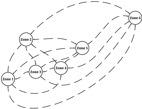
The University of Minnesota-Twin Cities (UMN) campus network is considered as the site on which to perform the test. The network we consider is partitioned into six zones. A digraph with $n=6$ vertices and $m=30$ links is produced by partitioning; the graph vertices are superimposed on the map shown in Fig. 1. It should be noted that the rebalancing performance is certainly affected by partitioning, but a detailed analysis is beyond the scope of this article.

Figure 1: The network zones.

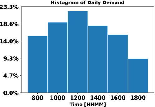
Figure 2 shows the histogram of the daily demand for UMN’s campuses. The peak occurs between 11:00 AM and 1:00 PM. Since the demand represents the intra-zonal trips on the campuses (not commutes to the campus), it does not necessarily follow the typical morning and afternoon peaks.

Figure 2: Histogram of the daily demand for the UMN’s campuses.

5.2 Case Study

A 12-hour historical trip dataset is considered for the case study. We consider each time step equal to two minutes. So, the number of iterations is 360. Some origin-destination pairs are used more frequently than others, which implies a significant imbalance in demand. The number of vehicles is constant at each time step (including equilibrium) and is equal to ${\bf 1}_{n}^{T}{p}\left(t\right)+{\bf 1}_{n(n-1)}^{T}{g}\left(t\right)$ ([13, 16]). Therefore, $\underline{M}={\bf 1}_{n(n-1)}^{T}{\bar{g}}={T^{T}}\left({{\lambda}}+{\bar{R}}\right)$ can be considered a lower band for the fleet size. The origin and destination of every trip in the travel data are subsequently assigned to the corresponding zones in the graph. We used Dijkstra’s algorithm [36] to compute the shortest path between the zone centers on a real road network (Google Maps). Initial conditions for the AMoD model are ${x}_{0}=\begin{bmatrix}0^{T}_{\frac{n(n-1)}{2}}&\frac{\underline{M}}{n}{1^{T}_{n}}&0^{T}_{\frac{n(n-1)}{2}}\end{bmatrix}^{T}$. In the performed simulation, no congestion effects have been considered, i.e., travel times are considered exogenous. If congestion is considered in the model, travel times are endogenous and a function of the policies performed by Algorithm 1. In that case, the model is no longer linear and a detailed analysis is beyond the scope of this article. The average queue length, the average number of rebalancing vehicles, and the average number of customer-carrying vehicles are the metrics that we are interested in investigating using Algorithm 1. The disturbance attenuation $\gamma$ is selected to be 0.1. Let $W_{\lambda}=0.01I$. Weights matrices $R_{x}$ and $R_{v}$ are chosen as $R_{x}=\begin{bmatrix}{\tilde{\bf\lambda}}&0&0\\ 0&0&0\\ 0&0&0\end{bmatrix}$ and $R_{v}=\begin{bmatrix}{\rho\tilde{T}}&0\\ 0&{\rho\tilde{T}}\end{bmatrix},$ where $\rho=0.05$. The reference being tracked ($\lambda$, ${\bar{R}}^{\star}$) is recomputed via Problem (25) every 2 hours (60 iterations). Therefore, $R_{x}$ will be changing every 60 iterations. The recursive least-squares algorithm is used to tune the parameters of the critic network online. The parameters of the actions networks are updated according to (11a) and (11b).

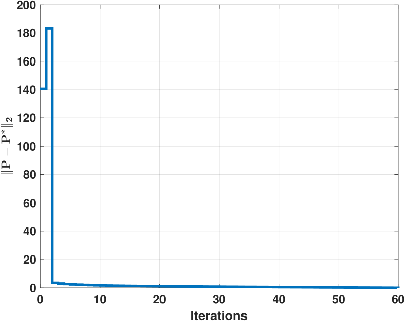
(a) Online convergence of $P$.

(b) Convergence of the control action network parameters ($K_{v}$).

(c) Convergence of the disturbance action network parameters ($K_{d}$).

Figure 3: Convergence of the parameters of actions and critic network.

The parameters of the critic and the actions networks are initialized to identity and zero, respectively. Based on this initialization step, the system dynamics move forward in time, and tuning the parameter structures is done by observing the states online. In the RLS problems, the persistency of the excitation condition required to converge the recursive least-squares tuning, i.e., avoiding the parameter drift problem, will hold. However, In Algorithm 1, the persistency of the excitation condition is only required for the initial iteration.

In the studied network depicted in Fig. 1, $m_{1}=66$, $m_{2}=60$, and $m_{3}=30$. Let’s denote $F_{\rm npe}$ the number of parameters estimated in the matrix $F$. So, $S_{\rm npe}=12246$, $P_{\rm npe}=2211$, ${K_{v},}_{\rm npe}=3960$, and ${K_{d},}_{\rm npe}=1800$.

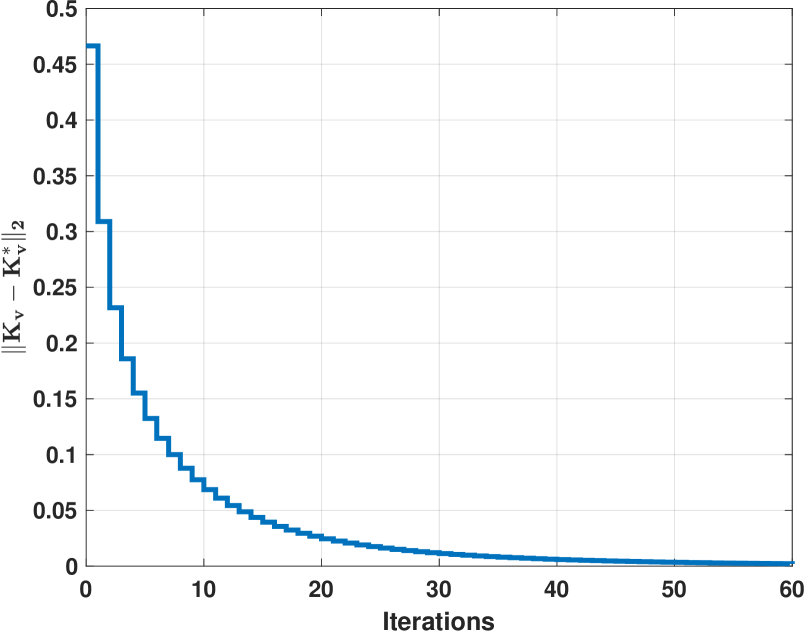
In Fig. 3(a), the convergence of the critic network is illustrated. Fig. 3(b) shows the convergence of the control action network, while Fig. 3(c) depicts the convergence of the disturbance action network.

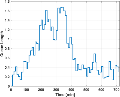
Figure 4 shows the average queue length over all origin-destinations. At the beginning of the peak hours, the queue length increases while after peak hours, it decreases remarkably. Note that each step of the trace in Figures 4, 5, and 6 represents ten minutes.

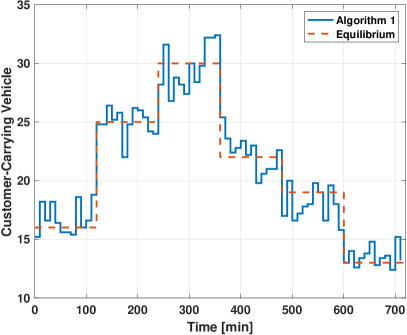
Figure 5 depicts the average customer-carrying vehicles in the network. The dashed (red) figure, shows the average of $\lambda$ over all origin-destinations. Note that we showed in Section 4 that $\bar{U}=\lambda$. Since the arrival of customers $d_{t}$ is given by the realization of a Poisson process of parameter $\lambda$, the expectation of the average customer-carrying vehicles on the links in the network tracks the average of $\lambda$.

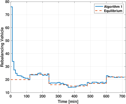
Figure 6 illustrates the average number of rebalancing vehicles over all origin-destinations. The dashed (red) figure, shows the average of ${{\bar{R}}^{\star}}$ over all origin-destinations obtained by (25). Similar to Fig. 5, since the arrival of customers $d_{t}$ is not deterministic, the expectation of the average number of rebalancing vehicles on the links in the network tracks the average of ${{\bar{R}}^{\star}}$. Moreover, the optimal rebalancing policy of Algorithm 1 changes over time due to the change in the demand during the different time intervals.

Figure 4: The average queue length.

Figure 5: The average customer-carrying vehicles.

Figure 6: The average rebalancing vehicles.

6 Conclusion

In this paper, we proposed a model-free, real-time, data-efficient Q-learning-based algorithm to solve the H_∞ control of linear discrete-time systems and applied it to AMoD systems modeled as a H_∞ control of the linear discrete-time system.

Besides presenting the algorithm, its convergence was discussed and proved. Afterward, we showed the parameters of the actions and critic networks converged to the optimal values. Numerical results from an AMoD system control in a real case study showed that the proposed algorithm can be implemented in high-dimension systems thanks to the quadratic computational complexity $\mathcal{O}({\underline{q}}^{2})$ and using only a single data point for updating the actor and critic networks in each iteration.

References

• [1] D. Q. Nguyen-Phuoc, M. Zhou, M. H. Chua, A. R. Alho, S. Oh, R. Seshadri, and D.-T. Le, “Examining the effects of automated mobility-on-demand services on public transport systems using an agent-based simulation approach,” Transportation Research Part A: Policy and Practice, vol. 169, p. 103583, 2023.
• [2] B. Turan, R. Pedarsani, and M. Alizadeh, “Dynamic pricing and fleet management for electric autonomous mobility on demand systems,” Transportation Research Part C: Emerging Technologies, vol. 121, p. 102829, 2020.
• [3] E. Skordilis, Y. Hou, C. Tripp, M. Moniot, P. Graf, and D. Biagioni, “A modular and transferable reinforcement learning framework for the fleet rebalancing problem,” IEEE Transactions on Intelligent Transportation Systems, 2021.
• [4] Y. Gao, D. Jiang, and Y. Xu, “Optimize taxi driving strategies based on reinforcement learning,” International Journal of Geographical Information Science, vol. 32, no. 8, pp. 1677–1696, 2018.
• [5] G. Guo and Y. Xu, “A deep reinforcement learning approach to ride-sharing vehicle dispatching in autonomous mobility-on-demand systems,” IEEE Intelligent Transportation Systems Magazine, vol. 14, no. 1, 2022.
• [6] C. Fluri, C. Ruch, J. Zilly, J. Hakenberg, and E. Frazzoli, “Learning to operate a fleet of cars,” in 2019 IEEE Intelligent Transportation Systems Conference (ITSC), pp. 2292–2298, IEEE, 2019.
• [7] A. O. Al-Abbasi, A. Ghosh, and V. Aggarwal, “Deeppool: Distributed model-free algorithm for ride-sharing using deep reinforcement learning,” IEEE Transactions on Intelligent Transportation Systems, vol. 20, no. 12, pp. 4714–4727, 2019.
• [8] K. Lin, R. Zhao, Z. Xu, and J. Zhou, “Efficient large-scale fleet management via multi-agent deep reinforcement learning,” in Proceedings of the 24th ACM SIGKDD International Conference on Knowledge Discovery & Data Mining, pp. 1774–1783, 2018.
• [9] M. Guériau and I. Dusparic, “Samod: Shared autonomous mobility-on-demand using decentralized reinforcement learning,” in 2018 21st International Conference on Intelligent Transportation Systems (ITSC), pp. 1558–1563, IEEE, 2018.
• [10] J. Wen, J. Zhao, and P. Jaillet, “Rebalancing shared mobility-on-demand systems: A reinforcement learning approach,” in 2017 IEEE 20th international conference on intelligent transportation systems (ITSC), pp. 220–225, Ieee, 2017.
• [11] R. Zhang, Models and Large-scale Coordination Algorithms for Autonomous Mobility-on-demand. Stanford University, 2016.
• [12] M. Volkov, J. Aslam, and D. Rus, “Markov-based redistribution policy model for future urban mobility networks,” in 2012 15th International IEEE Conference on Intelligent Transportation Systems, pp. 1906–1911, IEEE, 2012.
• [13] M. Pavone, S. L. Smith, E. Frazzoli, and D. Rus, “Robotic load balancing for mobility-on-demand systems,” The International Journal of Robotics Research, vol. 31, no. 7, pp. 839–854, 2012.
• [14] R. Zhang and M. Pavone, “Control of robotic mobility-on-demand systems: a queueing-theoretical perspective,” The International Journal of Robotics Research, vol. 35, no. 1-3, pp. 186–203, 2016.
• [15] F. Rossi, R. Zhang, Y. Hindy, and M. Pavone, “Routing autonomous vehicles in congested transportation networks: Structural properties and coordination algorithms,” Autonomous Robots, vol. 42, no. 7, pp. 1427–1442, 2018.
• [16] A. Carron, F. Seccamonte, C. Ruch, E. Frazzoli, and M. N. Zeilinger, “Scalable model predictive control for autonomous mobility-on-demand systems,” IEEE Transactions on Control Systems Technology, 2019.
• [17] Z. Lei, X. Qian, and S. V. Ukkusuri, “Efficient proactive vehicle relocation for on-demand mobility service with recurrent neural networks,” Transportation Research Part C: Emerging Technologies, vol. 117, p. 102678, 2020.
• [18] R. Iglesias, F. Rossi, K. Wang, D. Hallac, J. Leskovec, and M. Pavone, “Data-driven model predictive control of autonomous mobility-on-demand systems,” in 2018 IEEE international conference on robotics and automation (ICRA), pp. 6019–6025, IEEE, 2018.
• [19] M. Tsao, D. Milojevic, C. Ruch, M. Salazar, E. Frazzoli, and M. Pavone, “Model predictive control of ride-sharing autonomous mobility-on-demand systems,” in 2019 International Conference on Robotics and Automation (ICRA), pp. 6665–6671, IEEE, 2019.
• [20] R. S. Sutton and A. G. Barto, Reinforcement learning: An introduction. MIT press, 2018.
• [21] Y. Abbasi-Yadkori, N. Lazic, and C. Szepesvári, “Model-free linear quadratic control via reduction to expert prediction,” in The 22nd International Conference on Artificial Intelligence and Statistics, pp. 3108–3117, PMLR, 2019.
• [22] S. Dean, H. Mania, N. Matni, B. Recht, and S. Tu, “On the sample complexity of the linear quadratic regulator,” Foundations of Computational Mathematics, vol. 20, no. 4, pp. 633–679, 2020.
• [23] S. Tu and B. Recht, “Least-squares temporal difference learning for the linear quadratic regulator,” in International Conference on Machine Learning, pp. 5005–5014, PMLR, 2018.
• [24] N. Matni, A. Proutiere, A. Rantzer, and S. Tu, “From self-tuning regulators to reinforcement learning and back again,” in 2019 IEEE 58th Conference on Decision and Control (CDC), pp. 3724–3740, IEEE, 2019.
• [25] M. Fazel, R. Ge, S. Kakade, and M. Mesbahi, “Global convergence of policy gradient methods for the linear quadratic regulator,” in International Conference on Machine Learning, pp. 1467–1476, PMLR, 2018.
• [26] A. Al-Tamimi, F. L. Lewis, and M. Abu-Khalaf, “Model-free q-learning designs for linear discrete-time zero-sum games with application to h-infinity control,” Automatica, vol. 43, no. 3, pp. 473–481, 2007.
• [27] H.-N. Wu and B. Luo, “Neural network based online simultaneous policy update algorithm for solving the hji equation in nonlinear h control,” IEEE Transactions on Neural Networks and Learning Systems, vol. 23, no. 12, pp. 1884–1895, 2012.
• [28] B. Kiumarsi, F. L. Lewis, and Z.-P. Jiang, “H control of linear discrete-time systems: Off-policy reinforcement learning,” Automatica, vol. 78, pp. 144–152, 2017.
• [29] T. Baar and P. Bernhard, “If’-optimal control and related minimax design problems,” Birkh/iuser,, 1995.
• [30] A. Rantzer, “Minimax adaptive control for a finite set of linear systems,” in Learning for Dynamics and Control, pp. 893–904, PMLR, 2021.
• [31] K. Zhang, Z. Yang, and T. Basar, “Policy optimization provably converges to nash equilibria in zero-sum linear quadratic games,” Advances in Neural Information Processing Systems, vol. 32, 2019.
• [32] F. L. Lewis, D. Vrabie, and K. G. Vamvoudakis, “Reinforcement learning and feedback control: Using natural decision methods to design optimal adaptive controllers,” IEEE Control Systems Magazine, vol. 32, no. 6, pp. 76–105, 2012.
• [33] A. Goel, A. L. Bruce, and D. S. Bernstein, “Recursive least squares with variable-direction forgetting: Compensating for the loss of persistency [lecture notes],” IEEE Control Systems Magazine, vol. 40, no. 4, pp. 80–102, 2020.
• [34] J. Sherman and W. J. Morrison, “Adjustment of an inverse matrix corresponding to a change in one element of a given matrix,” The Annals of Mathematical Statistics, vol. 21, no. 1, pp. 124–127, 1950.
• [35] A. A. Stoorvogel and A. J. Weeren, “The discrete-time riccati equation related to the h/sub/spl infin//control problem,” IEEE Transactions on Automatic Control, vol. 39, no. 3, pp. 686–691, 1994.
• [36] E. W. Dijkstra et al., “A note on two problems in connexion with graphs,” Numerische mathematik, vol. 1, no. 1, pp. 269–271, 1959.