Learning a Stable Dynamic System with a Lyapunov Energy Function for Demonstratives Using Neural Networks

Abstract

Autonomous Dynamic System (DS)-based algorithms hold a pivotal and foundational role in the field of Learning from Demonstration (LfD). Nevertheless, they confront the formidable challenge of striking a delicate balance between achieving precision in learning and ensuring the overall stability of the system. In response to this substantial challenge, this paper introduces a novel DS algorithm rooted in neural network technology. This algorithm not only possesses the capability to extract critical insights from demonstration data but also demonstrates the capacity to learn a candidate Lyapunov energy function that is consistent with the provided data. The model presented in this paper employs a straightforward neural network architecture that excels in fulfilling a dual objective: optimizing accuracy while simultaneously preserving global stability. To comprehensively evaluate the effectiveness of the proposed algorithm, rigorous assessments are conducted using the LASA dataset, further reinforced by empirical validation through a robotic experiment.

I INTRODUCTION

The popularity of robotics is growing with advancements in technology, and robots are expected to possess greater intelligence to perform complex tasks comparable to those performed by humans. However, programming them, especially for non-experts, is challenging. In such situations, Learning from Demonstration (LfD) is a user-friendly approach where robots acquire skills by observing demonstrations without relying on an explicit script or defined reward functions [1].

In practical applications, achieving stability is crucial for ensuring that learned skills can effectively converge to the desired target state. Dynamic Systems (DS) represent powerful tools that offer a versatile solution for modeling trajectories and generating highly stable real-time motion, as highlighted in [2]. This superiority over traditional methods, such as interpolation techniques, underscores the value of DS in various contexts.

One notable advantage of Autonomous DS is their ability to encode the task’s target state as a stable attractor, making them inherently resilient to perturbations. Consequently, DS can formulate stable motions from any starting point within the robot’s workspace. This inherent stability facilitates seamless adaptation to new situations while maintaining robust performance. Furthermore, DS possess the capability to dynamically adjust the robot’s trajectory to accommodate changes in the target position or unexpected obstacles, as discussed in reference [3]. This adaptability further enhances their utility in real-world scenarios.

Given the paramount importance of stability, ensuring the stability of DS is a critical consideration. One elegant approach to guaranteeing stability involves introducing a Lyapunov function, which is a positive-definite, continuously differentiable energy function. This Lyapunov function serves as a robust means of ensuring stability. The first work that combines Lyapunov theorems with DS learning is known as the Stable Estimator of Dynamical Systems (SEDS) [2]. In SEDS, the objective is to learn a globally asymptotically stable DS, which is represented by Gaussian Mixture Models (GMM) and Gaussian Mixture Regression (GMR), while adhering to Lyapunov stability constraints.

However, it’s worth noting that the quadratic Lyapunov function utilized in SEDS can impose limitations on the accuracy of reproduction. Researchers have come to recognize that imposing overly strict stability constraints can curtail the accuracy of learning from demonstrations, leading to less precise reproductions. This trade-off between accuracy and stability is often referred to as the ”accuracy vs. stability dilemma.” [4].

To address the problem, researchers have proposed several modified approaches aimed at enhancing reproduction accuracy while adhering to stability constraints. One such approach is the Control Lyapunov Function-based Dynamics Movements (CLF-DMs) algorithm, introduced in [5]. This algorithm operates in three steps: In the first step, the algorithm learns a valid Lyapunov function that is approximately consistent with the provided data. In the second step, state-of-the-art regression techniques are employed to model an estimate of the motion based on the demonstrations. And the final step focuses on ensuring the stability of the reproduced motion in real-time by solving a constrained convex optimization problem.

While CLF-DM has the advantage of being able to learn from a broader set of demonstrations, it should be noted that the algorithm requires solving optimization problems in each step to maintain stability. This complexity and sensitivity to parameters are important considerations.

Another approach presented in reference [4] introduces a diffeomorphic transformation called ”$\tau$ -SEDS.” This transformation is designed to project the data into a different space, with the primary aim of improving accuracy while preserving the system’s stability.

Compared to traditional methods, neural network-based algorithms [6, 7, 8, 9, 10] have proven to be highly effective for learning from demonstrations. These neural networks can be thought of as versatile fitting functions, and when appropriately structured or constrained, they can generate trajectories that converge to satisfy a Lyapunov function. This Lyapunov function can either be learned by another neural network or manually designed. In the pursuit of improving accuracy in reproduction, some researchers have proposed neural networks dedicated to estimating the Lyapunov function based on demonstration data, as demonstrated in [11]. This approach helps enhance reproduction accuracy by reducing violations of the Lyapunov function observed in the demonstration data. However, despite these efforts, the simplicity of the neural network structure in [11] may still leave room for improvement in reproduction accuracy.

To address this limitation, references [6, 7, 8, 9, 10] have introduced invertible neural network structures. These structures are used to transform the original DS into a new, simplified DS that possesses inherent properties that ensure convergence to the target. The advantage of using invertible transformations is that the fitted DS inherits stability from the simplified DS. However, it’s important to note that invertible neural networks often have limitations in terms of their nonlinear fitting capabilities. To compensate for this, multiple layers of invertible neural networks may need to be stacked, which can increase computational costs and time.

To address the challenges commonly encountered by neural network-based algorithms, in this paper, a novel neural network-based approach is proposed that eliminates the need for invertible transformations. The key contributions of this paper are summarized as follows:

• A novel neural network architecture is proposed that is capable of directly learning a Lyapunov candidate function from demonstration data.

• The proposed neural network exhibits the ability to directly output state differentiations, aligning seamlessly with the requirements of DS. Leveraging the learned Lyapunov candidate function, the generated trajectories are guaranteed to converge to the desired target, offering enhanced stability and accuracy in the learning process.

• The experimental results conclusively show that the proposed algorithm possesses the versatility to not only learn effectively from a single demonstration but also learn from multiple demonstrations. This adaptability underscores the robustness and practicality of the proposed approach in a variety of learning scenarios.

The paper is organized as follows: Section II provides a comprehensive discussion of the problem formulations. In section III, the intricate details of the neural networks are presented. In section IV, the evaluation results of the proposed algorithm. This evaluation includes simulations conducted on various handwriting trajectories sourced from the Lasa datasets [12], as well as experiments carried out on the Franka Emika robot. In section V, the conclusion is made.

II Problem Formulation

When a person or a robot engages in a point-to-point task, the motions involved can often be effectively modeled using an autonomous DS as:

$$\dot{\boldsymbol{x}}=f(\boldsymbol{x}),\ \forall\boldsymbol{x}\in\mathbb{R}^{d},$$ (1)

where $f:\mathbb{R}^{d}\mapsto\mathbb{R}^{d}$ is a continuous and continuously differentiable function, which is described to have a single equilibrium state, denoted as $\boldsymbol{x}^{*}$. This equilibrium state corresponds to the target state of the task and can be considered as the attractor of the DS. To simplify the analysis and without sacrificing generality, the targets of the motions are assumed to be positioned at the origin of the Cartesian coordinate system by $\tilde{\boldsymbol{x}}=\boldsymbol{x}-\boldsymbol{x}^{*}$. Equation (1), which can also describe the manipulation skills acquired from demonstration data, yields a solution $\Phi(\boldsymbol{x}_{0},t)$ that represents a valid trajectory generated by the Autonomous DS when provided with an initial state $\boldsymbol{x}_{0}$. The ideal motions can then be obtained by adding this trajectory to the target state $\boldsymbol{x}=\tilde{\boldsymbol{x}}+\boldsymbol{x}^{*}$. Consequently, by altering the initial conditions $\boldsymbol{x}_{0}$, different solution trajectories leading to the target state $\boldsymbol{x}^{*}$ can be generated. This flexibility allows for various trajectories to be produced, each tailored to different initial conditions.

The demonstration data is typically recorded in the following format: $\begin{Bmatrix}\boldsymbol{x}_{k,n},\dot{\boldsymbol{x}}_{k,n}\ |\ k=1,2,...,K_{n};\ n=1,2,...,N_{d}\end{Bmatrix},$ where $n$ represents the index of the demonstrations and $k$ is the $k$-th sampling time. $N_{d}$ denotes the total number of demonstrations and $K_{n}\ (n=1,2,...,N_{d})$ represents the whole sampling number of the $n$-th demonstrated motion. The state variable $\boldsymbol{x}$ signifies the condition or configuration of either a human or a robot. Typically, in the context of robotic systems, it corresponds to the spatial coordinates of the robot’s end-effector. Alternatively, in the case of human involvement, it characterizes the spatial position of the human hand within Cartesian space. $\dot{\boldsymbol{x}}$ is the first-order time derivative of $\boldsymbol{x}$. Moreover, it’s important to note that all the demonstrations for a given task share the same target state. These demonstrations are assumed to align with an Autonomous DS as described in Equation (1). This alignment allows for the modeling of the system in a parametric fashion, which can be represented as:

$$\hat{\dot{\boldsymbol{x}}}=\hat{f}(\boldsymbol{x},\boldsymbol{\theta}),\ \forall\boldsymbol{x}\in\mathbb{R}^{d}.$$ (2)

where $\hat{\dot{\boldsymbol{x}}}$ denotes the estimate of $\dot{\boldsymbol{x}}$, $\hat{f}$ is the model designed manually to approximate the DS in (1), and $\boldsymbol{\theta}$ denotes the parameter in the model which can be learned. The optimal parameter configuration, denoted as $\boldsymbol{\theta^{*}}$, is obtained through the minimization of the following objective function:

$$J(\boldsymbol{\theta})\propto\sum_{n=1}^{N_{d}}\sum_{k=1}^{K_{n}}\left\|\hat{\dot{\boldsymbol{x}}}_{k,n}-\dot{\boldsymbol{x}}_{k,n}\right\|^{2},$$ (3)

where $\propto$ denotes the proportionality relation, $\left\|\cdot\right\|^{2}$ is the $l_{2}$-norm and $\hat{\dot{\boldsymbol{x}}}_{k,n}$ represents the estimate of $\dot{\boldsymbol{x}}_{k,n}$. Therefore, the objective function compels the learned model to generate precise reproductions that closely match the demonstrated behavior. Nonetheless, it’s crucial to note that the objective function alone does not guarantee the stability of the model. An Autonomous DS is considered locally asymptotically stable at the point $\boldsymbol{x}^{*}$ if a continuous and continuously differentiable Lyapunov candidate function $V(\boldsymbol{x}):\mathbb{R}^{d}\rightarrow\mathbb{R}$ exists, satisfying the following conditions:

$$\begin{cases}(a)V(\boldsymbol{x}^{*})=0,\\ (b)\dot{V}(\boldsymbol{x}^{*})=0,\\ (c)V(\boldsymbol{x})>0:\forall\boldsymbol{x}\neq\boldsymbol{x}^{*},\\ (d)\dot{V}(\boldsymbol{x})<0:\forall\boldsymbol{x}\neq\boldsymbol{x}^{*}.\end{cases}$$ (4)

Furthermore, if the radially unbounded condition as

$$\lim_{\left\|\boldsymbol{x}\right\|\rightarrow+\infty}V(\boldsymbol{x})=+\infty,$$ (5)

is satisfied, the DS is globally asymptotically stable.

Incorporating stability considerations into the DS learning process to ensure the robot’s arrival at the desired target state may impose limitations on model accuracy. This is because striving for accurate reproductions akin to the demonstration data might lead to violations of the pre-defined Lyapunov candidate function. However, deriving a suitable Lyapunov candidate function analytically from the demonstration data is a challenging task, rendering the search for a satisfactory solution quite difficult.

In this paper, a data-driven approach to learn the Lyapunov candidate function, utilizing neural networks is proposed. This method offers an alternative that bypasses the need for designing Lyapunov candidate function, facilitating the achievement of stability in the DS learning process, which is introduced in the following section.

III The Proposed Approach

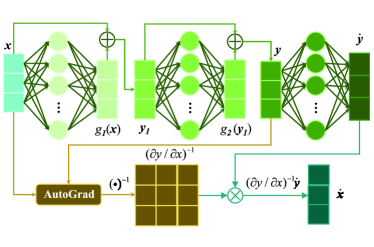
Figure 1: The overall structure of the proposed algorithm for learning a DS while simultaneously learning a Lyapunov energy function.

To construct a Lyapunov energy function, the most straightforward way is to establish it as:

$$V(\boldsymbol{x})=\frac{1}{2}\boldsymbol{x}^{\mathrm{T}}\boldsymbol{x}.$$ (6)

Given the universal fitting capabilities of neural networks, the candidate Lyapunov energy function can be formulated as follows:

$$V(\boldsymbol{x})=\frac{1}{2}g(\boldsymbol{x})^{\mathrm{T}}g(\boldsymbol{x}),$$ (7)

where $g$ is the function fitted by the neural networks. Denoting $\boldsymbol{y}=g(\boldsymbol{x})$ as shown in Fig. 1, equation 7 becomes:

$$V(\boldsymbol{x})=\frac{1}{2}\boldsymbol{y}^{\mathrm{T}}\boldsymbol{y}.$$ (8)

To ensure the stability of the system, it is essential to calculate the derivative of the energy function, which can be expressed as follows:

$$\dot{V}(\boldsymbol{x})=\boldsymbol{y}^{\mathrm{T}}\frac{\partial\boldsymbol{y}}{\partial\boldsymbol{x}}\dot{\boldsymbol{x}}.$$ (9)

When $\frac{\partial\boldsymbol{y}}{\partial\boldsymbol{x}}$ is invertible, $\dot{\boldsymbol{x}}$ can be calculated as:

$$\dot{\boldsymbol{x}}=(\frac{\partial\boldsymbol{y}}{\partial\boldsymbol{x}})^{-1}\dot{\boldsymbol{y}},$$ (10)

where $\dot{\boldsymbol{y}}$ is the designed variable in this paper. Substituting the designed $\dot{\boldsymbol{x}}$ into 9, the 9 becomes:

$$\dot{V}(\boldsymbol{x}) =\boldsymbol{y}^{\mathrm{T}}\frac{\partial\boldsymbol{y}}{\partial\boldsymbol{x}}(\frac{\partial\boldsymbol{y}}{\partial\boldsymbol{x}})^{-1}\boldsymbol{y}$$ (11)

$$=\boldsymbol{y}^{\mathrm{T}}\dot{\boldsymbol{y}}$$

Without loss of generality, the motion targets are positioned at the origin of the Cartesian coordinate system, and the convergence point of $\boldsymbol{y}$ also coincides with the origin. As a result, when the following conditions are met, the global stability of the DS is ensured.

• $\frac{\partial\boldsymbol{y}}{\partial\boldsymbol{x}}$ is invertible, which is the prerequisite condition of designing $\dot{\boldsymbol{x}}$.

• The appropriate $\dot{\boldsymbol{y}}$ to guarantee that $\boldsymbol{y}^{\mathrm{T}}\dot{\boldsymbol{y}}<0$, which is the required of the Lyapunov stability condition.

• Only the target point of $\boldsymbol{x}^{*}$ should map to the convergence point of $\boldsymbol{y}$. In cases where the transformation is not invertible, and multiple points of $\boldsymbol{x}$ map to the convergence point of $\boldsymbol{y}$, then there is a risk that the original DS may converge to an undesired equilibrium point, which can result in unintended behavior or outcomes.

The first problem can be readily addressed by employing a residual structure for the design of $\boldsymbol{y}$, defined as:

$$\boldsymbol{y}=m(\boldsymbol{x})+\boldsymbol{x},$$ (12)

where $m(\cdot)$ represents neural networks. In this context, the non-invertibility of $\frac{\partial\boldsymbol{y}}{\partial\boldsymbol{x}}$ occurs only when one of the eigenvalues of $\frac{\partial m(\boldsymbol{x})}{\partial\boldsymbol{x}}$ is equal to $-1$. However, this condition is highly unlikely when using neural network structures, making it a practical and effective solution.

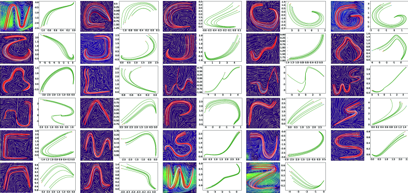
Figure 2: The simulation of the LASA dataset using the proposed algorithm is depicted. The images with a dark background showcase the learned vector fields. Within these vector field visuals, the white dotted lines represent the original demonstration data, while the red solid lines correspond to the reproductions, all originating from the same initial points. The target points are denoted as ”$x$” in these visuals. Furthermore, the transformed reproduction trajectories (consistent with $\boldsymbol{y}$ as shown in Fig. 1) are presented with white background. Within this context, the solid points indicate the starting positions for these trajectories.

The second problem can be solved directly by designing $\dot{\boldsymbol{y}}$ as $\dot{\boldsymbol{y}}=-{\boldsymbol{y}}$. An alternative method is to learn the $\dot{\boldsymbol{y}}$ using a neural network. To ensure compliance with the stability condition, it can be expressed as follows:

$$\dot{\boldsymbol{y}}=\begin{cases}n(\boldsymbol{y})\ \ \ \ \ \ if\ \boldsymbol{y}^{\mathrm{T}}n(\boldsymbol{y})<0,\\ -\beta\boldsymbol{y}\ \ \ \ \ \ \ \ \ otherwise,\end{cases}$$ (13)

where $n(\cdot)$ is a neural network and $\beta$ is a manually designed positive constant. Taking inspiration from the research conducted by [13] and simultaneously learning both $\dot{\boldsymbol{y}}$ and $\dot{\boldsymbol{x}}$, the equation (12) can be reformulated as:

$$\dot{\boldsymbol{y}}=n(\boldsymbol{y})-(n(\boldsymbol{y})+\beta\boldsymbol{y})\frac{\mathrm{Relu}(\boldsymbol{y}^{\mathrm{T}}n(\boldsymbol{y}))}{\boldsymbol{y}^{\mathrm{T}}n(\boldsymbol{y})},$$ (14)

where $\mathrm{Relu}$ is a element-wise calculated function characterized by the following form:

$$\mathrm{Relu}(s)=\begin{cases}s\ \ \ \ \ \ \ \ \ \mathrm{if}\ s>0,\\ 0\ \ \ \ \ \ \ \ \ \mathrm{otherwise}.\end{cases}$$ (15)

To address the third problem, the neural network structure can be configured in a way that ensures the output becomes a zero vector only when the input is a zero vector. There are two approaches to achieve this:

Firstly, employing a suitable activation function, such as $\mathrm{Softplus}$, that ensures the output is always greater than zero. Then, plus the output of the neural network with $\boldsymbol{x}$. Secondly, configure the neural network without bias but with an appropriate activation function, like $\mathrm{Tanh}$, to guarantee that the output is a zero vector when the input is a zero vector. Additionally, set a portion of the neural network’s weight matrices to be identity matrices. This ensures that the weight matrices are linearly independent and cannot produce a zero vector when the input is non-zero.

In our paper, both of these methods are utilized, and the expression for $\boldsymbol{y}$ corresponding with the illustration in Fig. 1 that is defined as follows:

$$\begin{cases}g_{1}(\boldsymbol{x})=m_{1}(\boldsymbol{x})\odot\boldsymbol{x},\\ \boldsymbol{y}_{1}=\boldsymbol{x}+g_{1}(\boldsymbol{x}),\\ g_{2}(\boldsymbol{y}_{1})=m_{2}(g_{1}(\boldsymbol{x})),\\ \boldsymbol{y}=g_{2}(\boldsymbol{y}_{1})+\boldsymbol{y}_{1}\end{cases}$$ (16)

where $\odot$ denotes Hadamard product, $m_{1}(\cdot)$ is the neural network with $\mathrm{Softplus}$ activation function and $m_{2}(\cdot)$ is the neural network with $\mathrm{Tanh}$ activation function and no bias. Then $\boldsymbol{y}$ is formulated as follows:

$$\boldsymbol{y}=\boldsymbol{x}+m_{1}(\boldsymbol{x}))\odot\boldsymbol{x}+m_{2}(m_{1}(\boldsymbol{x}))\odot\boldsymbol{x}+\boldsymbol{x})),$$ (17)

which is consistent with the setting as in equation (12).

Consequently, the proposed algorithm involves three neural networks: $m_{1}(\cdot)$, $m_{2}(\cdot)$, and $n(\cdot)$. And in this paper, all the neural networks are configured with three layers, and each layer of $m_{1}(\cdot)$ and $n(\cdot)$ comprises 20 neurons, while of $m_{2}(\cdot)$ comprises 40 neurons in this paper.

IV Experiment Results and Discussions

To comprehensively assess the efficacy of the proposed algorithm, a rigorous evaluation protocol encompassing both simulation and real-world experimentation has been implemented. The results are summarized as follows:

IV-A Simulation Results

The initial assessment of the proposed algorithm was carried out using the LASA dataset, which comprises a comprehensive collection of handwritten letter trajectories.

To evaluate the proposed algorithm, the quantitative evaluation of accuracy was performed through the application of two error metrics: the Swept Error Area (SEA) [5] and the Velocity Root Mean Square Error ($V_{rmse}$) [14]. The SEA scores serve as an indicator of the algorithm’s capability to faithfully replicate the shapes of the demonstrated motions. On the other hand, the $V_{rmse}$ metric gauges the algorithm’s proficiency in preserving the velocities of the demonstrated motions. A lower SEA score signifies superior accuracy in reproducing the trajectories with the same initial start points, while a lower $V_{rmse}$ value indicates that the reproductions closely match the smoothness of the original demonstrations. These metrics collectively assess the performance of the reproduced trajectories by quantifying their similarity to the demonstrated trajectories.

For the implementation of the proposed algorithm, the ”Adam” optimization method is opted, adhering to the default hyper-parameters. Specifically, the initial learning rate was set to $1\times 10^{-3}$, with a decay rate of $0.99$. Subsequently, the learned DS was utilized to generate trajectories originating from the same starting points with the same steps as demonstrations, facilitating an assessment of the trade-off between stability and accuracy. In this paper, all demonstration data from the LASA dataset were utilized, with trajectories generated from all available starting points. Prior to processing, the data underwent normalization, bringing it within the range of [$-1,1$]. The algorithm’s parameters were initialized with random values, and the maximum number of iterations was set to 2000, with a mini-batch size of 64. For the sake of equitable comparisons, DS algorithms that named SEDS and CLF-DM are chosen, for which source code was readily accessible. The parameters for these comparative algorithms were configured to match the values originally specified in their respective references, ensuring a fair benchmark.

Fig. 2 presents a visual representation of the vector fields (depicted with dark background) and the transformed trajectories generated by the proposed DS algorithm for 29 examples drawn from the LASA dataset. Notably, the reproduced trajectories (depicted in red) closely align with the original demonstrations (depicted in white). It is worth emphasizing that regardless of whether the initial point of the DS matches the starting point of the demonstrations, the reproduced DS consistently converges towards the intended goal. Furthermore, the last three images in the third row and first image in the fourth row of Fig. 2 illustrate more intricate motions. For instance, in the third image of the third row, three different types of demonstrations commence from distinct initial points but all culminate at the same target point, underscoring the algorithm’s versatility and effectiveness.

The quantified results are shown Table I, the results clearly demonstrate that the proposed algorithm outperforms other methods in terms of trajectory reproduction accuracy. Notably, the proposed algorithm achieves the highest SEA score and the best $V_{rmse}$ value, showcasing substantial improvements of approximately $15.56\%$ in SEA score and approximately $13.23\%$ in $V_{rmse}$ when compared to CLF-DM.

Furthermore, a noteworthy observation stems from the images presented in Fig. 2, characterized with white background, representing the transformed trajectories denoted as $\boldsymbol{y}$ in Fig. 1. To elucidate, considering the case of the letter ”J” for illustration. These transformed trajectories manage to retain certain essential characteristics of the original trajectories while scaling the two-dimensional coordinates to align with the simplest Lyapunov energy function. This innovative approach, albeit seemingly straightforward at first glance, yields intriguing results when addressing the problem at hand.

TABLE I: Reproduction error of different DS approaches on the LASA dataset

Learning method	Mean SEA($mm^{2}$)	Mean $V_{rmse}(mm/s)$
SEDS [2]	8.18 $\times$ 10^5	142.9
CLF-DM [5]	5.72 $\times$ 10^5	71.8
The proposed method	4.83 $\times$ 10^5	62.3

The proposed algorithm can also learn the vector field from one demonstration and four results are shown in Fig. 3. The results show that the proposed algorithm can learn from one demonstration well, and the vector field is similar to the vector field learned from multiply demonstrations, which is consistent with common sense.

Incorporating the direct design of $\dot{\boldsymbol{y}}$ as $\dot{\boldsymbol{y}}=-{\boldsymbol{y}}$ into the modeling approach is another method of simultaneously learning the stability DS with a Lyapunov energy function. In Fig. 5, the simulation results for the same data previously examined in Fig. 3 is presented using this approach. It becomes evident that the endpoints of the reproduced trajectories for $P$ and $S$ deviate slightly from the target point. This discrepancy implies that the reproduced velocities differ significantly from the demonstrated ones. Furthermore, the reproduction of $G$ does not align with the demonstrated trajectory. Consequently, this observation suggests that when employing this method, the model’s fitting capacity falls short of expectations.

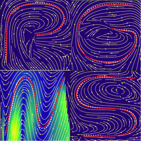
Figure 3: The simulation of learning from one demonstration using the proposed algorithm is depicted.

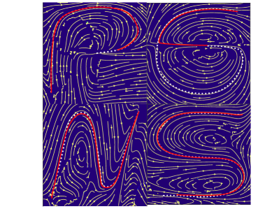
Figure 4: The simulation of learning from one demonstration without modeling the $\dot{\boldsymbol{y}}$ using the proposed algorithm is depicted.

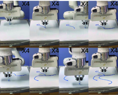
Figure 5: The real-world experiments involving the generation of multiple trajectories using the ”Multi-Models-1” dataset from LASA. These experiments employ the proposed algorithm for trajectory learning.

IV-B Validation on Robot

Experiments were conducted to validate the proposed algorithm using a Franka Emika robot. The model was trained using data from the ’Multi-Models-1’ subset of the LASA dataset, then it was executed on a whiteboard using a pen held by the robot.

Throughout the experiment, the robot continuously acquired its end-effector’s position and utilized the proposed algorithm to calculate the corresponding velocity.

To evaluate the algorithm’s performance, four random points on the whiteboard were selected. The results demonstrated that the proposed algorithm generated trajectories that converged toward manually defined target points. These trajectories closely followed the vector field, as illustrated in the third figure of the third row in Fig. 2.

V CONCLUSIONS

In this paper, a neural network-based algorithm designed for learning from single or multiple demonstrations is introduced. The algorithm’s performance is assessed through both simulated scenarios featuring diverse handwriting examples and practical experiments involving a physical robot. The experimental outcomes provide compelling evidence regarding the efficacy of the proposed method.

Nevertheless, it is crucial to acknowledge that the proposed algorithm relies on neural networks, and the model training process is comparatively time-consuming when compared to conventional DMPs or GMMs. This aspect presents an opportunity for future research, aimed at enhancing the algorithm’s efficiency and reducing its training time.

References

- [1] H. Ravichandar, A.S. Polydoros, and S. Chernova, ”Recent Advances in Robot Learning from Demonstration,” Annual Review of Control Robotics and Autonomous Systems, vol. 3, no. 1, pp. 297-330, 2020.
- [2] S.M. Khansari-Zadeh and A. Billard, ”Learning stable nonlinear dynamical systems with Gaussian mixture models,” IEEE Transactions on Robotics, vol. 27, no. 5, pp. 943-957, 2011.
- [3] M. Saveriano and D. Lee, ”Distance based dynamical system modulation for reactive avoidance of moving obstacles,” in Proceedings of International Conference on Robotics and Automation, Hong Kong, China, May, 2014, pp. 5618-5623.
- [4] K. Neumann and J.J. Steil, ”Learning robot motions with stable dynamical systems under diffeomorphic transformations,” Robotics and Autonomous Systems, vol. 70, pp. 1-15, 2015.
- [5] S.M. Khansari-Zadeh and A. Billard, ”Learning control Lyapunov function to ensure stability of dynamical system-based robot reaching motions,” Robotics and Autonomous Systems, vol. 62, no. 6, pp. 752- 765, 2014.
- [6] J. Urain, M. Ginesi, D. Tateo and J. Peters, ”ImitationFlow: Learning Deep Stable Stochastic Dynamic Systems by Normalizing Flows,” IEEE/RSJ International Conference on Intelligent Robots and Systems , Las Vegas, USA, 2020, pp. 5231-5237.
- [7] M.A. Rana, A. Li, D. Fox, B. Boots, F. Ramos, and N. Ratliff, ”Euclideanizing flows: Diffeomorphic reduction for learning stable dynamical systems,” in Proceedings of the 2nd Conference on Learning for Dynamics and Control, Online, June, 2020, pp. 630-639.
- [8] Y. Zhang, L. Cheng, H. Li and R. Cao, ”Learning Accurate and Stable Point-to-Point Motions: A Dynamic System Approach,” IEEE Robotics and Automation Letters, vol. 7, no. 2, pp. 1510-1517, 2022.
- [9] Y. Zhang, L. Cheng, R. Cao, H. Li and C. Yang, ”A neural network based framework for variable impedance skills learning from demonstrations,” Robotics and Autonomous Systems, vol. 160, no. 104312, 2023.
- [10] H. Zhang, L. Cheng, Y. Zhang, ”Learning Robust Point-to-Point Motions Adversarially: A Stochastic Differential Equation Approach,” IEEE Robotics and Automation Letters, vol. 8, no. 4, pp. 2357-2364, 2023.
- [11] K. Neumann, A. Lemme, and J.J. Steil, ”Neural learning of stable dynamical systems based on data-driven Lyapunov candidates,” in Proceedings of IEEE International Conference on Intelligent Robots and Systems, Tokyo, Japan, Nov. 2013, pp. 1216-1222.
- [12] Available: https://bitbucket.org/khansari/lasahandwritingdataset/
- [13] J.Z. Kolter and G. Manek, ”Learning Stable Deep Dynamics Models”, in Proceedings of Advances in Neural Information Processing System, vol. 32, pp. 11128-11136, 2019.
- [14] A. Lemme, F. Reinhart, K. Neumann, and J.J. Steil, ”Neural learning of vector fields for encoding stable dynamical systems,” Neurocomputing, vol. 141, pp. 3-14, 2014