Zhao

Adaptive Neyman Allocation

Adaptive Neyman Allocation

Jinglong ZhaoBoston University, Questrom School of Business, Boston, MA, 02215, jinglong@bu.edu

In experimental design, Neyman allocation refers to the practice of allocating subjects into treated and control groups, potentially in unequal numbers proportional to their respective standard deviations, with the objective of minimizing the variance of the treatment effect estimator. This widely recognized approach increases statistical power in scenarios where the treated and control groups have different standard deviations, as is often the case in social experiments, clinical trials, marketing research, and online A/B testing. However, Neyman allocation cannot be implemented unless the standard deviations are known in advance. Fortunately, the multi-stage nature of the aforementioned applications allows the use of earlier stage observations to estimate the standard deviations, which further guide allocation decisions in later stages. In this paper, we introduce a competitive analysis framework to study this multi-stage experimental design problem. We propose a simple adaptive Neyman allocation algorithm, which almost matches the information-theoretic limit of conducting experiments. Using online A/B testing data from a social media site, we demonstrate the effectiveness of our adaptive Neyman allocation algorithm, highlighting its practicality especially when applied with only a limited number of stages.

First draft: May 15, 2023. This version:

1 Introduction

Why are field experiments usually conducted with half-treated and half-control? One answer, dating back to Neyman (1934), is that experimenters usually believe the treated and control groups to have the same level of variability. When the treated and control groups have different levels of variability, such as an intervention in a social experiment triggers heterogeneity or even polarization of the outcomes (Duflo et al. 2007, Mosleh et al. 2021), the seminal work of Neyman (1934) recommends an unequal allocation: the sizes of the treated and control groups should be proportional to their respective standard deviations. This approach has later on been recognized as “Neyman allocation.”

Neyman allocation has many desirable properties. First, since it prescribes the sizes of the treated and control groups, it can be naturally combined with complete randomization (Fisher 1936, Cox and Reid 2000, Imbens and Rubin 2015). Randomization then serves as the basis of validity for many randomized experiments (Cook et al. 2002, Deaton 2010). Second, it proves to minimize the variance of the widely-used difference-in-means estimator, and increases the statistical power in scenarios where the the treated and control groups have different levels of variability (Neyman 1934). Consequently, it brings tremendous value to a wide range of applications whose treatment and control groups have different standard deviations, such as social experiments (Duflo et al. 2007, Karlan and Zinman 2008, Yang et al. 2022), clinical trials (Berry 2006, Hu and Rosenberger 2003, Rosenberger and Lachin 2015), marketing research (Rossi and Allenby 2003, Sandor and Wedel 2001), and online A/B testing (Bakshy et al. 2014, Deng et al. 2013, Kohavi and Longbotham 2017). For example, at a social media site who compares two advertisement strategies, the standard deviation of the treated group is a half of that of the control groups; see Table 1 for the summary statistics.

Summary statistics of the number of clicks per million impressions at a social media site Mean St dev Min Median Max Treated $34176$ $12256$ $14732$ $31358$ $75752$ Control $53618$ $24850$ $20757$ $48796$ $162068$ Note: The data source of this table will be introduced in Section 7. In this data, the labels of treatment and control are masked; we only know that they refer to two different advertisement strategies.

Albeit useful, a challenge in using Neyman allocation arises when the standard deviations of the treated and control groups are unknown in advance. Fortunately, the multi-stage nature of the aforementioned applications allows the use of earlier stage observations to estimate the standard deviations. If the earlier stage observations suggest a higher level of variability in one group, more experimental subjects will be randomly allocated to the same group in the later stages, so that the confidence intervals of the average outcomes are roughly equal between the two groups. We refer to this approach as “adaptive Neyman allocation.”

In this paper, we study the optimal adaptive Neyman allocation problem.

To study this problem, we borrow the competitive analysis framework, which is a common optimization framework in the literature of decision-making under uncertainty. To the best of our knowledge, we are the first to introduce the competitive analysis framework into experimental designs. In the single-stage setup, an immediate implication of adopting this framework is an assumption-free result that half-treated-half-control allocations are optimal, without knowing the standard deviations of the treated and control groups, or any assumptions about these standard deviations. In the multi-stage setup, this framework allows for meaningful comparisons across different problem instances, even if the standard deviations of the treated and control groups are different. This is in contrast to the conventional minimax framework or the regret minimization framework, as the objective values in such frameworks will change under re-scaling of the standard deviations. To facilitate such comparisons, the minimax framework and the regret minimization framework need to assume the standard deviations being constants.

Another remarkable advantage of using the competitive analysis framework is that it facilitates a more precise examination of the second-order efficiency of experimental designs, which is different from the conventional emphasis on the first-order efficiency such as in Armstrong (2022) and Hahn et al. (2011). More specifically, when a total of $T$ experimental subjects are enrolled over $M\geq 2$ stages, the adaptive Neyman allocation algorithm in this paper achieves $1+O(T^{-\frac{M-1}{M}})$ competitiveness against a hindsight benchmark that knew the standard deviations in advance. In contrast, Armstrong (2022) show that when there are $M=2$ stages and when the first stage pilot experiment involves approximately $T^{\alpha}$ subjects, any value of $\alpha$ less than 1 will be first-order efficient. This means that, while two different parameterizations of $\alpha$ may both satisfy the first-order efficiency criterion, they can still lead to significantly different performances due to their second-order gap. This gap can lead to non-negligible impacts on cost reductions in social experiments and clinical trials, and on rapid product iterations in marketing research and online A/B testing.

Our work presents how to choose the sample size for each stage, and provides a simple and efficient adaptive Neyman allocation algorithm. In the $M=2$ stage example above, the optimal sample size for the first stage pilot experiment should involve approximately $T^{\frac{1}{2}}$ subjects, i.e., $\alpha=\frac{1}{2}$. In general, in an $M$ stage experiment, the optimal sample size for the $m$-th stage should involve approximately $T^{\frac{m}{M}}$ subjects, leading to an exponentially increasing number of subjects in the later stages of the experiment. This exponentially increasing pattern serves as a rule of thumb for practitioners who would like to conduct multi-stage experiments.

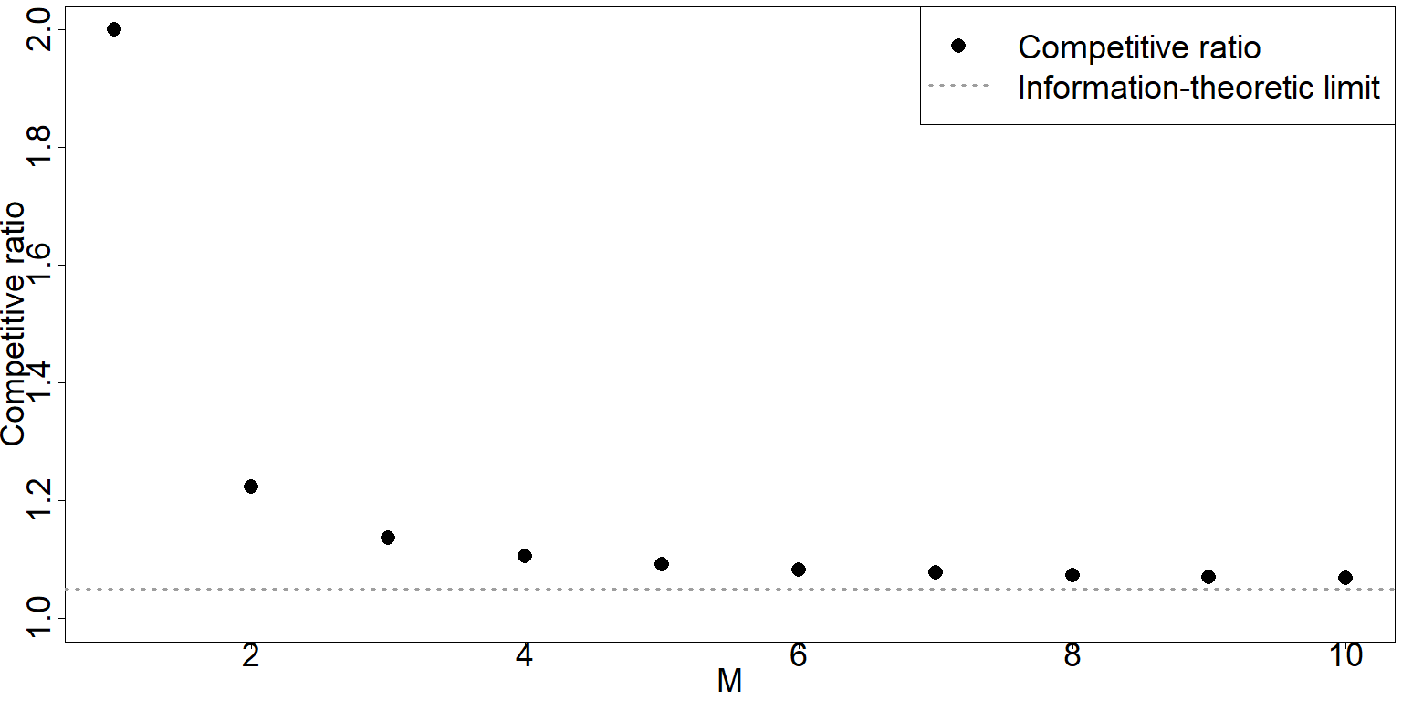
Figure 1: Competitive ratios with respect to the number of stages $M$

Recall that the competitive ratio of the aforementioned adaptive Neyman allocation algorithm is $1+O(T^{-\frac{M-1}{M}})$, which quickly approaches $1+O(T^{-1})$, the information-theoretic limit of conducting experiments when the number of stages is large. Combining these two results, it shows that the adaptive Neyman allocation algorithm is second-order efficient when the number of stages is large. See Figure 1 for an illustration. To the best of our knowledge, the best known result that studies a very similar yet different question in the literature (Antos et al. 2010, Carpentier and Munos 2011, Grover 2009) translates into a $1+O(T^{-\frac{1}{2}})$ ratio, and conjectures that this ratio is best-possible. Our results negate this conjecture by improving this ratio.

Our results have two practical implications. First, conducting a two-stage or three-stage experiment can be sufficiently efficient as long as the sample size in each stage approximately follows an exponentially increasing pattern. Even though the two-stage or three-stage experiment is not second-order efficient, having the ability to adaptively adjust the allocation of subjects based on insights from earlier stages of the experiment can greatly improve efficiency. Second, if there is existing experimental data available, practitioners can use it as the first stage experiment to estimate the levels of variability from the treated and control groups, and guide the allocation of subjects in later stages and improve efficiency.

Other Related Literature

The results in this paper are related to, but different from the following three lines of literature.

• Adaptive stratified sampling / active learning: in the simulations literature, the adaptive stratified sampling problem refers to adaptively sampling from fixed strata, with an objective of minimizing the estimation error (Asmussen and Glynn 2007, Glasserman 2004, Ross 2013, Etoré and Jourdain 2010, Etoré et al. 2011). The same problem is also referred to as the active learning problem (Antos et al. 2010, Carpentier and Munos 2011, Grover 2009, Russac et al. 2021). These problems have a very similar objective as the one considered in this paper. Our results improve the best known results under a weaker assumption than the literature, negating the conjecture that existing results are best-possible. The key to this improvement lies in explicitly using the uni-modal structure of the objective function.

  Another two closely related works are Armstrong (2022) and Hahn et al. (2011), in which they study this problem from a first-order efficiency perspective. Although a partial motivation is to guide pilot experimental studies, their results do not guide the selection of sample sizes, as any sample size is first-order efficient under their frameworks. In contrast, the competitive analysis framework in this paper enables us to study the second-order efficiency, which explicitly guides the selection of sample sizes in pilot experimental studies.

• Best-arm identification: in the online learning literature, the best-arm identification problem refers to adaptively sampling from a set of arms, with an objective of maximizing the probability of correctly identifying the arm with the largest mean outcome (Adusumilli 2022, Audibert et al. 2010, Kasy and Sautmann 2021, Kato et al. 2022, Mannor and Tsitsiklis 2004, Qin et al. 2017, Russo 2016). When there are only two arms (Adusumilli 2022, Audibert et al. 2010), the best-arm identification problem reduces to the adaptive stratified sampling problem, and our results improve the existing results. When there are at least three arms, there is one major difference: in the best-arm identification problem, the arms with smaller mean outcomes are less explored, and hence may have wider confidence intervals; whereas in our problem, we estimate the mean outcomes uniformly well across all arms.

• Stochastic multi-armed bandits: in the online learning literature, the stochastic multi-armed bandit problem refers to adaptively exploring-while-exploiting a set of arms, with an objective of maximizing the cumulative rewards (Lattimore and Szepesvári 2020, Slivkins 2019, Chen et al. 2022, Agrawal and Goyal 2012, Audibert et al. 2009, Auer et al. 2002, Garivier and Cappé 2011, Lai and Robbins 1985, Robbins 1952, Russo et al. 2018, Simchi-Levi and Wang 2023, Thompson 1933). There are many significant differences between our work and this line of literature. One of them lies in that there is no exploitation component in our problem, i.e., we consider a pure-exploration problem.

Roadmap

The paper is structured as follows. In Section 2 we formally introduce adaptive Neyman allocation. In Section 3 we introduce an optimization framework. As an immediate implication, we show that without making any assumptions, the classical half-half allocation is optimal under this optimization framework. In Sections 4 and 5 we study the two-stage and multi-stage adaptive Neyman allocation problem, respectively. In Section 6 we study some extensions of our results. In Section 7 we use online A/B testing data from a social media site to demonstrate the effectiveness of our adaptive Neyman allocation algorithm. In Section 8 we conclude the paper and point out the limitations and future research directions. All the proofs are deferred to the Online Appendix.

2 Problem Setup

Consider the following problem. There is a discrete, finite time horizon of $T\in\mathbb{N}$ periods. The time horizon $T$ stands for the size of the experiment, and is known to the experimenter before the start of the horizon. At any time $t\in[T]:=\{1,2,...,T\}$, one subject is involved in the experiment. We interchangeably use subject $t$ to stand for the subject that arrives at time $t$.

Let there be two versions of treatments. We use “treatment” and “control”, or $1$ and $0$, respectively, to stand for these two versions of treatments. Let $W_{t}\in\{0,1\}$ stand for the treatment assignment that subject $t$ receives. Following convention, we use $W_{t}$ for a random treatment assignment, and $w_{t}$ for one realization.

Following the potential outcomes framework and under the Stable Unit Treatment Value Assumption (Rubin 1974, Holland 1986, Imbens and Rubin 2015), each subject $t$ has a set of potential outcomes $Y_{t}(\cdot)$. Each observed outcome is related to its respective potential outcomes $Y_{t}=Y_{t}(w)$, if $W_{t}=w$. We assume the existence of a super-population (Abadie et al. 2020), such that each subject’s potential outcomes $(Y_{t}(1),Y_{t}(0))$ are independent and identically distributed (i.i.d.) replicas of a pair of representative random variables $(Y(1),Y(0))$. These random variables are drawn from a joint distribution of the super-population, i.e., $(Y(1),Y(0))\sim\mathcal{F}$. We put no restrictions on the correlation between $Y(1)$ and $Y(0)$.

In this paper, we consider a multi-stage randomized experiment, which we refer to as “adaptive Neyman allocation.” The experiment is conducted in $M\in\mathbb{N}$ stages. In stage $m\in[M]$, the experimenter conducts a completely randomized experiment parameterized by $(T_{m}(1),T_{m}(0))$. The size of the stage-$m$ experiment is $T_{m}=T_{m}(1)+T_{m}(0)$, and the experimenter randomly chooses exactly $T_{m}(1)$ subjects to receive treatment, and exactly $T_{m}(0)$ subjects to receive control. After $M$ stages of experiments, the experimenter has assigned $T(1)=\sum_{m=1}^{M}T_{m}(1)$ subjects to receive treatment, and $T(0)=\sum_{m=1}^{M}T_{m}(0)$ subjects to receive control. See Table 2 for a summary of notations.

Summary of notations Stage $1$ Stage $2$ $\ldots$ Stage $M$ Total Treated $T_{1}(1)$ $T_{2}(1)$ $\ldots$ $T_{M}(1)$ $T(1)$ Control $T_{1}(0)$ $T_{2}(0)$ $\ldots$ $T_{M}(0)$ $T(0)$ Total $T_{1}$ $T_{2}$ $\ldots$ $T_{M}$ $T$

Due to the adaptive nature of the experiment, $(T_{m}(1),T_{m}(0))$ could possibly depend on the treatment assignments and the observed outcomes in the earlier stages. The experimenter’s decisions are to adaptively choose the numbers of treated and control subjects $(T_{m}(1),T_{m}(0))$ for each stage, subject to the constraint that the numbers of treated and control subjects should sum up to the size of the experiment, i.e., $T(1)+T(0)=T$. Abstractly, we refer to a design of experiment $\eta$ as a policy that, at the beginning of each stage $m$, maps the treatment assignments and the observed outcomes in stages $1\sim(m-1)$ to a pair of $(T_{m}(1),T_{m}(0))$, and conducts a completely randomized experiment parameterized by $(T_{m}(1),T_{m}(0))$.

The causal effect of interest is the average treatment effect of the super-population,

$$\tau=\mathrm{E}[Y(1)-Y(0)].$$

After collecting data from the experiment, the experimenter uses the simple difference-in-means estimator to estimate the causal effect,

$$\widehat{\tau}=\frac{1}{T(1)}\sum_{t:W_{t}=1}Y_{t}-\frac{1}{T(0)}\sum_{t:W_{t}=0}Y_{t}.$$ (1)

It is worth mentioning that $\widehat{\tau}$ is random in nature. The randomness comes from two sources: the treatment assignments are random, and the potential outcomes are also random.

To evaluate the quality of the difference-in-means estimator, we consider the mean squared error of the estimator. When $T(1)$ and $T(0)$ are fixed, the mean squared error is equivalent to the variance of the estimator, which could be further expressed as follows,

$$\mathrm{E}\left[(\widehat{\tau}-\tau)^{2}\right]=\mathrm{Var}(\widehat{\tau})=\frac{1}{T(1)}\sigma^{2}(1)+\frac{1}{T(0)}\sigma^{2}(0),$$

where $\sigma(1),\sigma(0)>0$ stand for the standard deviations of the two representative random variables $Y(1)$ and $Y(0)$, respectively. When $T(1)$ and $T(0)$ are not fixed, but are adaptively determined depending on the observed outcomes in the previous stages, the mean squared error may not always be equal to the above expression. This issue has been recognized in the simulations literature when people discuss the bias in estimating confidence intervals (Ross 2013). We acknowledge that this is a potential limitation of our paper, and discuss this issue in more details in Section 8.

In this paper, we refer to the above expression as the proxy mean squared error.

$$V(T(1),T(0))=\frac{1}{T(1)}\sigma^{2}(1)+\frac{1}{T(0)}\sigma^{2}(0).$$ (2)

The experimenter’s objective is then to minimize the expected proxy mean squared error as defined above, $\mathrm{E}[V(T(1),T(0))]$, where the expectation is taken with respect to the randomness of the observed outcomes which then makes the adaptive decisions $(T(1),T(0))$ random.

One benefit of using the proxy mean squared error is that the proxy mean squared error only depends on $(T(1),T(0))$ the numbers of treated and control subjects in total. Even though the experimenter adaptively chooses $(T_{m}(1),T_{m}(0))$ in each stage and $(T(1),T(0))$ are adaptively determined, the proxy mean squared error (2) is still well-defined. The proxy mean squared error is a simple and effective proxy of the mean squared error. In the simulations literature, prior works have focused on minimizing this proxy mean squared error instead of the true mean squared error (Antos et al. 2010, Carpentier and Munos 2011, Grover 2009).

Under the proxy mean squared error, what is important is the total number of treated and control subjects. The multi-stage experiment enables the experimenter to make better choices for $(T(1),T(0))$ by appropriately selecting $(T_{m}(1),T_{m}(0))$ at each stage. In the following section, we will present an optimization framework for making such decisions.

3 An Optimization Framework

If the experimenter was endowed with clairvoyant information about the standard deviations $\sigma(1)$ and $\sigma(0)$, the experimenter would allocate $(T(1),T(0))$ optimally in a single-stage experiment to minimize $V(T(1),T(0))$. The optimal solution can be explicitly calculated as,

$$T^{*}(1)=\ \frac{\sigma(1)}{\sigma(1)+\sigma(0)}T, T^{*}(0)=\ \frac{\sigma(0)}{\sigma(1)+\sigma(0)}T,$$

and the optimal proxy mean squared error is given by the following expression,

$$V(T^{*}(1),T^{*}(0))=\frac{1}{T}(\sigma(1)+\sigma(0))^{2}.$$ (3)

This is what Neyman (1934) suggests, and has been recognized as Neyman allocation. As the standard deviations were assumed given, the original work of Neyman allocation only focused on single stage experiments. In this paper, we consider a more common setting where the standard deviations are not given. The experimenter makes decisions $(T(1),T(0))$ under uncertainty about $\sigma(1)$ and $\sigma(0)$.

In practice, the experimenter is more often not endowed with clairvoyant information about $\sigma(1)$ and $\sigma(0)$. As one common strategy of decision-making under uncertainty, we introduce the competitive analysis framework to experimental design. For any design of experiment $\eta$, let $(T^{\eta}(1),T^{\eta}(0))$ be the numbers of treated and control subjects assigned by policy $\eta$. The competitive analysis framework suggests to solve the following problem,

$$\inf_{\eta}\ \sup_{\sigma(1),\sigma(0)}\ \frac{\mathrm{E}[V(T^{\eta}(1),T^{\eta}(0))]}{V(T^{*}(1),T^{*}(0))}.$$ (4)

The above framework is similar to the minimax decision rule in the literature (Berger 2013, Bickel and Doksum 2015, Li 1983, Wu 1981). Yet it provides a tractable solution concept when the traditional minimax objective scales with the adversarial decisions. The optimal value to problem (4) is often referred to as a competitive ratio (Borodin and El-Yaniv 2005, Buchbinder et al. 2009).

As an illustration of the competitive analysis framework, consider the setup of the traditional single-stage Neyman allocation, but with unknown standard deviations. In the single stage experiment, the policy $\eta$ only determines one single and fixed pair of $(T(1),T(0))$. We replace the policy $\eta$ with this pair of actions $(T(1),T(0))$ in (4), and solve the new problem to optimal. This yields the following result, the proof of which is deferred to Section 10.3 in the Online Appendix.

Theorem 3.1

The optimal solution to

$$\inf_{T(1),T(0)}\ \sup_{\sigma(1),\sigma(0)}\ \frac{V(T(1),T(0))}{V(T^{*}(1),T^{*}(0))}$$

is given by $T(1)=T(0)=T/2$. Under this optimal solution,

$$\sup_{\sigma(1),\sigma(0)}\ \frac{V(\frac{T}{2},\frac{T}{2})}{V(T^{*}(1),T^{*}(0))}=2,$$

where the supremum is taken when either $\sigma(1)=0$ or $\sigma(0)=0$.

Theorem 3.1 re-produces the classical result that the optimal design involves an equal number of treated and control subjects (Neyman 1934). But Theorem 3.1 does not require any knowledge of the standard deviations of the treatment or control populations. More importantly, Theorem 3.1 does not even require any assumption, such as the treatment or control populations having the same support (see, e.g., Bojinov et al. (2023)), or the treatment effects being additive (which implies the standard deviations are the same, see, e.g., Wu (1981)), or permutation invariance (see, e.g., Basse et al. (2023)).

In other experimental design literature, Theorem 3.1 is often presented as an assumption and serves as the basis for designing optimal experiments (Bai 2022, Candogan et al. 2021, Greevy et al. 2004, Harshaw et al. 2019, Lu et al. 2011, Rosenbaum 1989, Xiong et al. 2019, 2022, Zhao and Zhou 2022). In contrast, by using the competitive analysis framework, Theorem 3.1 establishes the credibility of such an assumption.

In the following sections, we will use this competitive analysis framework to study adaptive Neyman allocation. We will start with the two-stage adaptive Neyman allocation to introduce the basic estimation ideas and build some intuitions in Section 4. We will then introduce the more general multi-stage adaptive Neyman allocation in Section 5.

4 Two-Stage Adaptive Neyman Allocation

In this section, we focus on the $M=2$ case, which we refer to as the two-stage adaptive Neyman allocation. When there are two stages, the experimental data collected during the first stage reveals information about the magnitudes of $\sigma(1)$ and $\sigma(0)$, which can be used to guide the design of the second stage experiment.

The algorithm.

Recall that $(T_{1}(1),T_{1}(0))$ stand for the numbers of treated and control subjects in the first stage, respectively, and that $T_{1}=T_{1}(1)+T_{1}(0)$ stands for the total number of subjects in the first stage. We consider the following sample variance estimators at the end of the first stage,

$$\widehat{\sigma}^{2}_{1}(1)= \ \frac{1}{T_{1}(1)-1}\sum_{\begin{subarray}{c}1\leq t\leq T_{1}\\ t:W_{t}=1\end{subarray}}\bigg{(}Y_{t}-\frac{1}{T_{1}(1)}\sum_{\begin{subarray}{c}1\leq t\leq T_{1}\\ t:W_{t}=1\end{subarray}}Y_{t}\bigg{)}^{2},$$ (5a)

$$\widehat{\sigma}^{2}_{1}(0)= \ \frac{1}{T_{1}(0)-1}\sum_{\begin{subarray}{c}1\leq t\leq T_{1}\\ t:W_{t}=0\end{subarray}}\bigg{(}Y_{t}-\frac{1}{T_{1}(0)}\sum_{\begin{subarray}{c}1\leq t\leq T_{1}\\ t:W_{t}=0\end{subarray}}Y_{t}\bigg{)}^{2}.$$ (5b)

After obtaining the sample variance estimators, it is natural to use such sample variance estimators to guide the Neyman allocation in the second stage. The allocation of treated and control subjects should roughly follow the ones suggested by (3), but the estimated standard deviations from the first stage will be used instead of the true standard deviations, i.e.,

$$T(1)=\ \frac{\widehat{\sigma}_{1}(1)}{\widehat{\sigma}_{1}(1)+\widehat{\sigma}_{1}(0)}T, T(0)=\ \frac{\widehat{\sigma}_{1}(0)}{\widehat{\sigma}_{1}(1)+\widehat{\sigma}_{1}(0)}T.$$ (6)

Based on this natural intuition, we define the two-stage adaptive Neyman allocation in Algorithm 1.

Algorithm 1 Two-stage adaptive Neyman allocation

Input: Tuning parameter $\beta$.

1:Initialize: $(T_{1}(1),T_{1}(0))\leftarrow(\frac{\beta}{2}\sqrt{T},\frac{\beta}{2}\sqrt{T})$.

2:Conduct a completely randomized experiment parameterized by $(T_{1}(1),T_{1}(0))$; $\triangleright$ Stage 1 experiment

3:Calculate two estimators $\widehat{\sigma}^{2}_{1}(1)$ and $\widehat{\sigma}^{2}_{1}(0)$ as defined in (5a) and (5b).

4:Case 1: $\frac{\widehat{\sigma}_{1}(1)}{\widehat{\sigma}_{1}(1)+\widehat{\sigma}_{1}(0)}T>\frac{\beta}{2}\sqrt{T}$ and $\frac{\widehat{\sigma}_{1}(0)}{\widehat{\sigma}_{1}(1)+\widehat{\sigma}_{1}(0)}T>\frac{\beta}{2}\sqrt{T}$

5:for $(T_{2}(1),T_{2}(0))\leftarrow(\frac{\widehat{\sigma}_{1}(1)}{\widehat{\sigma}_{1}(1)+\widehat{\sigma}_{1}(0)}T-\frac{\beta}{2}\sqrt{T},\frac{\widehat{\sigma}_{1}(0)}{\widehat{\sigma}_{1}(1)+\widehat{\sigma}_{1}(0)}T-\frac{\beta}{2}\sqrt{T})$.

6:Case 2: $\frac{\widehat{\sigma}_{1}(1)}{\widehat{\sigma}_{1}(1)+\widehat{\sigma}_{1}(0)}T\leq\frac{\beta}{2}\sqrt{T}$

7:for $(T_{2}(1),T_{2}(0))\leftarrow(0,T-\beta\sqrt{T})$.

8:Case 3: $\frac{\widehat{\sigma}_{1}(0)}{\widehat{\sigma}_{1}(1)+\widehat{\sigma}_{1}(0)}T\leq\frac{\beta}{2}\sqrt{T}$

9:for $(T_{2}(1),T_{2}(0))\leftarrow(T-\beta\sqrt{T},0)$.

10:Conduct a completely randomized experiment parameterized by $(T_{2}(1),T_{2}(0))$; $\triangleright$ Stage 2 experiment

In words, the experiment consists of two stages. In the first stage, the experiment has a total size of $\sqrt{T}$, and assigns half subjects to treated and the other half to control. Then we calculate the sample variance estimators $\widehat{\sigma}^{2}_{1}(1)$ and $\widehat{\sigma}^{2}_{1}(0)$. If neither $\widehat{\sigma}_{1}(1)$ or $\widehat{\sigma}_{1}(0)$ is too small, the second stage experiment roughly mimics the Neyman allocation by using the estimated variances. If $\widehat{\sigma}_{1}(1)$ or $\widehat{\sigma}_{1}(0)$ is too small, the second stage experiment assigns all subjects to control or treated, respectively.

In essence, the two-stage adaptive Neyman allocation is similar to the design in Hahn et al. (2011). But there are two differences. First and more importantly, we specify the optimal size for the first-stage experiment. Second, we use equation (6) to guide the allocation of treated and control subjects for the entire horizon; whereas Hahn et al. (2011) uses equation (6) to guide the allocation for the second stage.

Analysis.

We now present the first formal analysis about the quality of the two-stage adaptive Neyman allocation. Recall that the sample variance estimators are unbiased, i.e., $\mathrm{E}[\widehat{\sigma}^{2}_{1}(1)]=\sigma^{2}(1)$ and $\mathrm{E}[\widehat{\sigma}^{2}_{1}(0)]=\sigma^{2}(0)$. To ensure that the distributions of the sample variance estimators are concentrated enough around the true variances $\sigma^{2}(1)$ and $\sigma^{2}(0)$, we make the following assumption.

There exist two constants $\kappa(1),\kappa(0)<\infty$ which do not depend on $T$, such that

$$\kappa(1)=\frac{\mathrm{E}\left[(Y(1)-\mathrm{E}Y(1))^{4}\right]}{\sigma^{4}(1)}, \kappa(0)=\frac{\mathrm{E}\left[(Y(0)-\mathrm{E}Y(0))^{4}\right]}{\sigma^{4}(0)}.$$

Assumption 4 asserts that the representative random variables $Y(1),Y(0)$ are sufficiently light-tailed, in the sense that their respective kurtosis values $\kappa(1),\kappa(0)$ exist. It is worth noting that the kurtosis values are always greater than $1$, i.e., $\kappa(1),\kappa(0)>1$. For a Gaussian random variable $Z$, its kurtosis is equal to $3$, i.e., $\mathrm{E}\left[(Z-\mathrm{E}Z)^{4}\right]/\sigma^{4}(Z)=3$. The kurtosis will be larger for distributions with heavier tails, and smaller for those with lighter tails. In other papers, instead of assuming Assumption 4, either sub-Gaussianity or boundedness is often assumed (Lattimore and Szepesvári 2020, Slivkins 2019).

With the above assumption, we now show the quality of the two-stage adaptive Neyman allocation, as measured by the competitive ratio, in Theorem 4.1.

Theorem 4.1

Let $T\geq 16$ and $\varepsilon\in\left(0,\frac{1}{8}\right)$. Let $\beta=1$ in Algorithm 1. Let $(T(1),T(0))$ be the number of total treated and control subjects from Algorithm 1, respectively. Under Assumption 4, there exists an event that happens with probability at least $1-(\kappa(1)+\kappa(0))T^{-\varepsilon}$, conditional on which

$$\sup_{\sigma(1),\sigma(0)}\ \frac{V(T(1),T(0))}{V(T^{*}(1),T^{*}(0))}\leq 1+T^{-\frac{1}{2}+\varepsilon}.$$

Theorem 4.1 presents a high probability bound. Using an assumption that enables us to show exponentially small probability, we will be able to show that a similar bound (up to some logarithm factors) holds in expectation. See Corollary 6.1 in Section 6.

Results that study the quality of adaptive allocation policies also frequently appear in the active learning literature (Antos et al. 2010, Carpentier and Munos 2011, Grover 2009, Russac et al. 2021). This literature adopts a minimax regret framework, which differs from the competitive analysis framework. The minimax regret framework focuses on the difference between the variance of any policy and the optimal variance, rather than the ratio between them. As the magnitudes of $\sigma(1)$ and $\sigma(0)$ directly impact the objective value, the minimax regret framework typically assumes $\sigma(1)$ and $\sigma(0)$ are on the same order, which is not necessary in this paper. After translating into the framework of this paper, the best competitive ratio suggested by the literature is on the order of $1+O(T^{-\frac{1}{2}})$, using much more complicated and fully adaptive experimental designs such as upper confidence bound approaches. In contrast, Theorem 4.1 shows that a simple two-stage adaptive Neyman allocation can achieve the same competitive ratio, by adapting only once.

In Section 5, we will show that conducting experiments in more than two stages can improve the competitive ratio, to an extent that almost matches the information-theoretic limit of conducting adaptive experiments.

To conclude this section, we sketch some unrigorous intuitions behind the proof of Theorem 4.1 below, and defer the complete proof to Section 10.4 in the Online Appendix.

Proof 4.2

Sketch proof of Theorem 4.1. Denote $\rho=\frac{\sigma(1)}{\sigma(0)}$. Without loss of generality assume $\rho\geq 1$. Suppose the length of the first stage is parameterized by $T^{\alpha}$ (we ignore $\beta$ in this unrigorous sketch proof). We aim to find the optimal length $T^{\alpha}$ of the first stage.

Case 1: $\rho>\frac{T-T^{\alpha}}{T^{\alpha}}$. Then with high probability, the first stage reveals this condition and Algorithm 1 stops allocating subjects to the control group in the second stage. In this case, we will show that

$$\frac{V(T(1),T(0))}{V(T^{*}(1),T^{*}(0))}=\frac{T}{T-T^{\alpha}}\cdot\frac{\rho^{2}}{(\rho+1)^{2}}+\frac{T}{T^{\alpha}}\cdot\frac{1}{(\rho+1)^{2}}\leq\frac{T}{T-T^{\alpha}}\approx 1+T^{\alpha-1}.$$

Case $2$: $1\leq\rho\leq\frac{T-T^{\alpha}}{T^{\alpha}}$. Then with high probability, the first stage reveals this condition and Algorithm 1 mimics the Neyman allocation by using the estimated variances. In this case, we will show that

$$\frac{V(T(1),T(0))}{V(T^{*}(1),T^{*}(0))}\leq 1+\frac{\rho}{(\rho+1)^{2}}\cdot T^{-\alpha}\approx 1+T^{-\alpha}.$$

Combining both cases, we set $\alpha-1=-\alpha$ and obtain $\alpha=\frac{1}{2}$, which leads to competitive ratio $\frac{V(T(1),T(0))}{V(T^{*}(1),T^{*}(0))}\approx 1+T^{-\frac{1}{2}}.$

5 Multi-Stage Adaptive Neyman Allocation

This section presents an extension of the two-stage adaptive Neyman allocation to multiple stages. We provide a formal analysis of the competitive ratio of the multi-stage adaptive Neyman allocation, and show that such a competitive ratio is nearly optimal.

The algorithm.

The multi-stage adaptive Neyman allocation algorithm uses the following sample variance estimators at the end of each stage. Recall that $(T_{m}(1),T_{m}(0))$ stand for the numbers of treated and control subjects in stage $m$, respectively, and that $T_{m}=T_{m}(1)+T_{m}(0)$ stands for the total number of subjects in stage $m$. At the end of stage $m$, define the following sample variance estimators,

$$\widehat{\sigma}^{2}_{m}(1)= \ \frac{1}{\sum_{l=1}^{m}T_{l}(1)-1}\sum_{\begin{subarray}{c}1\leq t\leq\sum_{l=1}^{m}T_{l}\\ t:W_{t}=1\end{subarray}}\bigg{(}Y_{t}-\frac{1}{\sum_{l=1}^{m}T_{l}(1)}\sum_{\begin{subarray}{c}1\leq t\leq\sum_{l=1}^{m}T_{l}\\ t:W_{t}=1\end{subarray}}Y_{t}\bigg{)}^{2},$$ (7a)

$$\widehat{\sigma}^{2}_{m}(0)= \ \frac{1}{\sum_{l=1}^{m}T_{l}(0)-1}\sum_{\begin{subarray}{c}1\leq t\leq\sum_{l=1}^{m}T_{l}\\ t:W_{t}=0\end{subarray}}\bigg{(}Y_{t}-\frac{1}{\sum_{l=1}^{m}T_{l}(0)}\sum_{\begin{subarray}{c}1\leq t\leq\sum_{l=1}^{m}T_{l}\\ t:W_{t}=0\end{subarray}}Y_{t}\bigg{)}^{2}.$$ (7b)

Using the above sample variance estimators (7a) and (7b), we could update the allocation of treated and control subjects following the Neyman allocation, i.e.,

$$T(1)=\ \frac{\widehat{\sigma}_{m}(1)}{\widehat{\sigma}_{m}(1)+\widehat{\sigma}_{m}(0)}T, T(0)=\ \frac{\widehat{\sigma}_{m}(0)}{\widehat{\sigma}_{m}(1)+\widehat{\sigma}_{m}(0)}T.$$ (8)

We can update the above Neyman allocation as defined in (8) using the estimated variances at the end of each stage $m$. Using (8) we define the $M$-stage adaptive Neyman allocation. See Algorithm 2 for Pseudo-codes.

Algorithm 2 $M$-stage adaptive Neyman allocation

Inputs: Tuning parameters $\beta_{1},\beta_{2},...,\beta_{M-1},\beta_{M}=1$. $\triangleright$ There are $M$ pre-determined stages $[0,\beta_{1}T^{\frac{1}{M}}]$, $(\beta_{1}T^{\frac{1}{M}}$, $\beta_{2}T^{\frac{2}{M}}]$, …, $(\beta_{M-1}T^{\frac{M-1}{M}},T]$

1:Initialize: $(T_{1}(1),T_{1}(0))\leftarrow(\frac{\beta_{1}}{2}T^{\frac{1}{M}},\frac{\beta_{1}}{2}T^{\frac{1}{M}})$;

2:for $m=1,2,...,M-2$ do $\triangleright$ The $m$-th stage experiment

3:    Conduct a completely randomized experiment parameterized by $(T_{m}(1),T_{m}(0))$;

4:    Estimate $\widehat{\sigma}^{2}_{m}(1)$ and $\widehat{\sigma}^{2}_{m}(0)$ as in (7a) and (7b) using data collected during stages $1\sim m$;

5:    Case 1: $\frac{\widehat{\sigma}_{m}(0)}{\widehat{\sigma}_{m}(1)+\widehat{\sigma}_{m}(0)}T<\frac{\beta_{m}}{2}T^{\frac{m}{M}}$

6:    for For any $l\geq m+1$, $(T_{l}(1),T_{l}(0))\leftarrow(\beta_{l}T^{\frac{l}{M}}-\beta_{l-1}T^{\frac{l-1}{M}},0)$;

7:    for go to Line 30;

8:    Case 2: $\frac{\beta_{m}}{2}T^{\frac{m}{M}}\leq\frac{\widehat{\sigma}_{m}(0)}{\widehat{\sigma}_{m}(1)+\widehat{\sigma}_{m}(0)}T<\frac{\beta_{m+1}}{2}T^{\frac{m+1}{M}}$

9:    for $(T_{m+1}(1),T_{m+1}(0))\leftarrow(\beta_{m+1}T^{\frac{m+1}{M}}-\frac{\widehat{\sigma}_{m}(0)}{\widehat{\sigma}_{m}(1)+\widehat{\sigma}_{m}(0)}T-\frac{\beta_{m}}{2}T^{\frac{m}{M}},\frac{\widehat{\sigma}_{m}(0)}{\widehat{\sigma}_{m}(1)+\widehat{\sigma}_{m}(0)}T-\frac{\beta_{m}}{2}T^{\frac{m}{M}})$;

10:    for For any $l\geq m+2$, $(T_{l}(1),T_{l}(0))\leftarrow(\beta_{l}T^{\frac{l}{M}}-\beta_{l-1}T^{\frac{l-1}{M}},0)$;

11:    for go to Line 30;

12:    Case 3: $\frac{\widehat{\sigma}_{m}(0)}{\widehat{\sigma}_{m}(1)+\widehat{\sigma}_{m}(0)}T\geq\frac{\beta_{m+1}}{2}T^{\frac{m+1}{M}}$ and $\frac{\widehat{\sigma}_{m}(1)}{\widehat{\sigma}_{m}(1)+\widehat{\sigma}_{m}(0)}T\geq\frac{\beta_{m+1}}{2}T^{\frac{m+1}{M}}$

13:    for $(T_{m+1}(1),T_{m+1}(0))\leftarrow(\frac{\beta_{m+1}}{2}T^{\frac{m+1}{M}}-\frac{\beta_{m}}{2}T^{\frac{m}{M}},\frac{\beta_{m+1}}{2}T^{\frac{m+1}{M}}-\frac{\beta_{m}}{2}T^{\frac{m}{M}})$; $\triangleright$ Note: there is no “go to”

14:    Case 4: $\frac{\beta_{m}}{2}T^{\frac{m}{M}}\leq\frac{\widehat{\sigma}_{m}(1)}{\widehat{\sigma}_{m}(1)+\widehat{\sigma}_{m}(0)}T<\frac{\beta_{m+1}}{2}T^{\frac{m+1}{M}}$

15:    for $(T_{m+1}(1),T_{m+1}(0))\leftarrow(\frac{\widehat{\sigma}_{m}(1)}{\widehat{\sigma}_{m}(1)+\widehat{\sigma}_{m}(0)}T-\frac{\beta_{m}}{2}T^{\frac{m}{M}},\beta_{m+1}T^{\frac{m+1}{M}}-\frac{\widehat{\sigma}_{m}(1)}{\widehat{\sigma}_{m}(1)+\widehat{\sigma}_{m}(0)}T-\frac{\beta_{m}}{2}T^{\frac{m}{M}})$;

16:    for For any $l\geq m+2$, $(T_{l}(1),T_{l}(0))\leftarrow(\beta_{l}T^{\frac{l}{M}}-\beta_{l-1}T^{\frac{l-1}{M}},0)$;

17:    for go to Line 30;

18:    Case 5: $\frac{\widehat{\sigma}_{m}(1)}{\widehat{\sigma}_{m}(1)+\widehat{\sigma}_{m}(0)}T<\frac{\beta_{m}}{2}T^{\frac{m}{M}}$

19:    for For any $l\geq m+1$, $(T_{l}(1),T_{l}(0))\leftarrow(0,\beta_{l}T^{\frac{l}{M}}-\beta_{l-1}T^{\frac{l-1}{M}})$;

20:    for go to Line 30;

21:if $m=M-1$ then $\triangleright$ The $(M-1)$-th stage experiment

22:    Conduct a completely randomized experiment parameterized by $(T_{M-1}(1),T_{M-1}(0))$;

23:    Estimate $\widehat{\sigma}^{2}_{M-1}(1)$ and $\widehat{\sigma}^{2}_{M-1}(0)$ as in (7a) and (7b) using data collected during stages $1\sim(M-1)$;

24:    Case 1: $\frac{\widehat{\sigma}_{M-1}(0)}{\widehat{\sigma}_{M-1}(1)+\widehat{\sigma}_{M-1}(0)}T<\frac{\beta_{M-1}}{2}T^{\frac{M-1}{M}}$

25:    for $(T_{M}(1),T_{M}(0))\leftarrow(T-\beta_{M-1}T^{\frac{M-1}{M}},0)$;

26:    Case 2: $\frac{\widehat{\sigma}_{M-1}(0)}{\widehat{\sigma}_{M-1}(1)+\widehat{\sigma}_{M-1}(0)}T\geq\frac{\beta_{M-1}}{2}T^{\frac{M-1}{M}}$ and $\frac{\widehat{\sigma}_{M-1}(1)}{\widehat{\sigma}_{M-1}(1)+\widehat{\sigma}_{M-1}(0)}T\geq\frac{\beta_{M-1}}{2}T^{\frac{M-1}{M}}$

27:    for $(T_{M}(1),T_{M}(0))\leftarrow(\frac{\widehat{\sigma}_{M-1}(1)}{\widehat{\sigma}_{M-1}(1)+\widehat{\sigma}_{M-1}(0)}T-\frac{\beta_{M-1}}{2}T^{\frac{M-1}{M}},\frac{\widehat{\sigma}_{M-1}(0)}{\widehat{\sigma}_{M-1}(1)+\widehat{\sigma}_{M-1}(0)}T-\frac{\beta_{M-1}}{2}T^{\frac{M-1}{M}})$;

28:    Case 3: $\frac{\widehat{\sigma}_{M-1}(1)}{\widehat{\sigma}_{M-1}(1)+\widehat{\sigma}_{M-1}(0)}T<\frac{\beta_{M-1}}{2}T^{\frac{M-1}{M}}$

29:    for $(T_{M}(1),T_{M}(0))\leftarrow(0,T-\beta_{M-1}T^{\frac{M-1}{M}})$;

30:for $m^{\prime}=m+1,...,M$ do $\triangleright$ A sub-routine for experiments in the remaining stages

31:    Conduct a completely randomized experiment parameterized by $(T_{m^{\prime}}(1),T_{m^{\prime}}(0))$;

The $M$-stage adaptive Neyman allocation generalizes the idea of two-stage adaptive Neyman allocation: we use the observations in the earlier stages to estimate the variances, and use the estimated variances to guide the allocation in the later stages. Initially, an equal number of treated and control subjects are allocated in the first stage. At the end of each stage, sample variances are estimated using (7a) and (7b), and the number of treated and control subjects is determined using the Neyman allocation formula, as shown in (8).

There are three major cases that will happen. First, the estimated standard deviations $\widehat{\sigma}_{m}(1)$ and $\widehat{\sigma}_{m}(0)$ indicate that there is already an excessive allocation to either the treated or control group by the end of stage $m$. In this case, we immediately stop allocating subjects to that group in the subsequent stages. See Case 1 (Line 5) and Case 5 (Line 18) in Algorithm 2. Intuitively, we are pruning the corner cases: once we have used a small number of stages to identify that the standard deviation $\sigma(1)$ or $\sigma(0)$ is very small, we stop allocating subjects to that group.

Second, the estimated standard deviations $\widehat{\sigma}_{m}(1)$ and $\widehat{\sigma}_{m}(0)$ indicate that we have not allocated too many subjects to both groups by the end of stage $m$, but an equal allocation in the next stage $(m+1)$ would result in an excessive allocation to either the treated or control group. In this case, we follow the Neyman allocation in the next stage $(m+1)$ only. We then stop allocating subjects to that treated or control group in the subsequent stages after the next stage. See Case 2 (Line 8) and Case 4 (Line 14) in Algorithm 2. This is the non-trivial generalization from Algorithm 1 in the two-stage adaptive Neyman allocation. Intuitively, we are pruning the corner cases as early as possible: now that we have identified that the standard deviation $\sigma(1)$ or $\sigma(0)$ is small enough, we do not spend an extra stage to allocate more subjects than necessary and convince ourselves that they are small. Instead, we follow the Neyman allocation in the next stage, and, without even updating the estimators $\widehat{\sigma}_{m+1}(1)$ and $\widehat{\sigma}_{m+1}(0)$, directly stop allocating future subjects to that group.

Third, the estimated standard deviations $\widehat{\sigma}_{m}(1)$ and $\widehat{\sigma}_{m}(0)$ indicate that even with an equal allocation in the next stage, we will not have allocated too many subjects to both groups. In this case, we keep an equal allocation in the next stage. See Case 3 (Line 12) in Algorithm 2. Intuitively, we have not identified a significant difference between the standard deviation $\sigma(1)$ or $\sigma(0)$, so we keep a balanced exploration. After collecting data from the next stage, the above procedure is repeated.

Analysis.

Such a simple idea leads to an effective improvement over the two-stage adaptive Neyman allocation. We show the quality of the multi-stage adaptive Neyman allocation, as measured by the competitive ratio, in Theorem 5.1 below.

Theorem 5.1

Let $M\geq 3$, $T\geq 16$, and $0<\varepsilon\leq\min\{\frac{1}{M},\frac{1}{100}\}$. Let the tuning parameters from Algorithm 2 be defined as $\beta_{m}=6\cdot 15^{-\frac{m}{M}}$. Under these parameters, Algorithm 2 is feasible, i.e., $1<\beta_{1}T^{\frac{1}{M}}<...<\beta_{M-1}T^{\frac{M-1}{M}}<T$. Furthermore, let $(T(1),T(0))$ be the total number of treated and control subjects from Algorithm 2, respectively. Under Assumption 4, there exists an event that happens with probability at least $1-(M-1)(\kappa(1)+\kappa(0))T^{-\varepsilon}$, conditional on which

$$\sup_{\sigma(1),\sigma(0)}\ \frac{V(T(1),T(0))}{V(T^{*}(1),T^{*}(0))}\leq 1+4\cdot 15^{-\frac{1}{M}}T^{-\frac{M-1}{M}+\varepsilon}.$$

Theorem 5.1 presents a high probability bound. Using an assumption that enables us to show exponentially small probability, we will be able to show that a similar bound (up to some logarithm factors) holds in expectation. See Corollary 6.2 in Section 6. This result improves the best existing results in the literature (Antos et al. 2010, Carpentier and Munos 2011, Grover 2009), and negates the conjecture that the competitive ratio is lower bounded by $1+\Omega(T^{-\frac{1}{2}})$. We sketch some unrigorous intuitions behind the proof of Theorem 5.1 below. The proof borrows ideas from Adusumilli (2022), Simchi-Levi and Wang (2023), Perchet et al. (2016), Zhang et al. (2020). We defer the complete proof to Section 10.5 in the Online Appendix.

Proof 5.2

Sketch proof of Theorem 5.1. Denote $\rho=\frac{\sigma(1)}{\sigma(0)}$. Without loss of generality assume $\rho\geq 1$. Suppose there are $(M-1)$ constants $0\leq\alpha_{1}\leq\alpha_{2}\leq\ldots\leq\alpha_{M-1}\leq 1$, such that we can choose the lengths of the $M$ stages to be roughly in the following order: $[0,T^{\alpha_{1}}]$, $(T^{\alpha_{1}},T^{\alpha_{2}}]$, …, $(T^{\alpha_{M-1}},T]$.

Case 1: $\rho>\frac{T-T^{\alpha_{1}}}{T^{\alpha_{1}}}$. Then with high probability, the first stage reveals this condition and the algorithm stops allocating subjects to the control group from the second stage. In this case, we will show that

$$\frac{V(T(1),T(0))}{V(T^{*}(1),T^{*}(0))}=\frac{T}{T-T^{\alpha_{1}}}\cdot\frac{\rho^{2}}{(\rho+1)^{2}}+\frac{T}{T^{\alpha_{1}}}\cdot\frac{1}{(\rho+1)^{2}}\leq\frac{T}{T-T^{\alpha_{1}}}\approx 1+T^{\alpha_{1}-1}.$$

Case $m$ $(2\leq m\leq M-1)$: $\frac{T-T^{\alpha_{m}}}{T^{\alpha_{m}}}<\rho\leq\frac{T-T^{\alpha_{m-1}}}{T^{\alpha_{m-1}}}$. Then with high probability, this condition is not revealed until the end of the $(m-1)$-th stage. One this condition is revealed, the algorithm allocates a few subjects to the control group in the $m$-th stage, and stops allocating subjects to the control group from the $(m+1)$-th stage. In this case, we will show that

$$\frac{V(T(1),T(0))}{V(T^{*}(1),T^{*}(0))}\leq 1+\frac{\rho}{(\rho+1)^{2}}\cdot T^{-\alpha_{m-1}}\approx 1+T^{\alpha_{m}-\alpha_{m-1}-1}.$$

Case $M$: $1\leq\rho\leq\frac{T-T^{\alpha_{M-1}}}{T^{\alpha_{M-1}}}$. Then with high probability, this condition is not revealed until the end of the $(M-1)$-th stage. In the last stage, the algorithm mimics Neyman allocation by using the estimated variances. In this case, we will show that

$$\frac{V(T(1),T(0))}{V(T^{*}(1),T^{*}(0))}\leq 1+\frac{\rho}{(\rho+1)^{2}}\cdot T^{-\alpha_{M-1}}\approx 1+T^{-\alpha_{M-1}}.$$

Combining all cases, we solve

$$\min_{\alpha_{1},...,\alpha_{M-1}}\max\{\alpha_{1}-1,\alpha_{2}-\alpha_{1}-1,...,-\alpha_{M-1}\}$$

and obtain $\alpha_{m}=\frac{m}{M}$, which leads to competitive ratio $\frac{V(T(1),T(0))}{V(T^{*}(1),T^{*}(0))}\approx 1+T^{-\frac{M-1}{M}}.$

Information-theoretic limit.

Next, we present an information-theoretic limit of such experiments, as measured by the competitive ratio, in Theorem 5.3 below.

Theorem 5.3

Let $T\geq 4$. For any adaptive design of experiment $\eta$, let $(T^{\eta}(1),T^{\eta}(0))$ be the total number of treated and control subjects from $\eta$, respectively. There exists a problem instance such that on this problem instance,

$$\frac{\mathrm{E}[V(T^{\eta}(1),T^{\eta}(0))]}{V(T^{*}(1),T^{*}(0))}\geq 1+\frac{1}{480}T^{-1}.$$

We sketch some unrigorous intuitions behind the proof of Theorem 5.3 as follows, and defer the complete information-theoretic proof of Theorem 5.3 to Section LABEL:sec:proof:thm:LB in the Online Appendix.

Proof 5.4

Sketch proof of Theorem 5.3. To prove Theorem 5.3, we construct two probability distributions $\nu$ and $\nu^{\prime}$ that are challenging to distinguish. Define $\epsilon=\frac{1}{3T^{\frac{1}{2}}}.$ Both distributions have three discrete supports $\{-1,0,1\}$. The probability mass for distribution $\nu$ is given by

$$p_{-1}=\frac{1}{3}, p_{0}=\frac{1}{3}, p_{1}=\frac{1}{3}.$$

The probability mass for distribution $\nu^{\prime}$ is given by

$$p^{\prime}_{-1}=\frac{1}{3}+\frac{\epsilon}{2}, p^{\prime}_{0}=\frac{1}{3}-\epsilon, p^{\prime}_{1}=\frac{1}{3}+\frac{\epsilon}{2}.$$

Then we bound the KL-divergences of these two probability distributions,

$$D_{KL}(\nu||\nu^{\prime})\leq\frac{9}{2}\epsilon^{2}=\frac{1}{2T}, D_{KL}(\nu^{\prime}||\nu)\leq\frac{9}{2}\epsilon^{2}=\frac{1}{2T}.$$

Intuitively, it is challenging to distinguish the above two probability distributions within $T$ rounds. This means that, any policy can not distinguish the above two probability distributions until the end of horizon. Since the two probability distributions are not distinguishable, the best policy in this situation has to follow the half-half allocation, which leads to a competitive ratio $\frac{\mathrm{E}[V(T^{\eta}(1),T^{\eta}(0))]}{V(T^{*}(1),T^{*}(0))}\approx 1+T^{-1}.$

By comparing Theorems 5.1 and 5.3, we see that when $M$, the number of stages, is large, the two results are close to each other. When there are $\log(T)$ many stages, the two results almost match with each other, suggesting that the multi-stage adaptive Neyman allocation is the optimal design of experiments, whose competitive ratio almost matches the information-theoretic limit of conducting adaptive experiments.

6 Extensions

In the previous sections, we have seen that Theorems 4.1 and 5.1 provide high probability bounds for the competitive ratios of using adaptive Neyman allocation. But with low probability, the competitive ratios might be much larger. In this section, we show that similar bounds as in Theorems 4.1 and 5.1 still hold in expectation.

We will need a stronger assumption to show that the low probability events happen with exponentially small probability. But this stronger assumption is still weaker than the standard modeling assumptions that commonly appear in the active learning literature, where existing works assume that both the standard deviations and the supports are bounded (Antos et al. 2010, Carpentier and Munos 2011, Grover 2009).

There exists a constant $C<\infty$ which does not depend on $T$, such that

$$|Y(1)|\leq C\sigma(1), |Y(0)|\leq C\sigma(0).$$

Assumption 6 asserts that the representative random variables $Y(1),T(0)$ have bounded supports that depend on the variances. In contrast, the traditional literature sometimes assumes that the bounded support is between $[0,1]$, and that the variances are constants. To illustrate Assumption 6, consider the following example. Consider a three-point distribution $Z$, such that with probability $1-2p$, $Z=0$; with probability $p$, $Z=1$; and with probability $p$, $Z=-1$. In this example, $|Z|\leq 1$ and $\sigma(Z)=\sqrt{2p}$. If $p\approx\frac{1}{T}$, then Assumption 6 does not hold. On the other hand, if $p=\frac{1}{3}$, then Assumption 6 holds with constant $C=\sqrt{\frac{3}{2}}$.

Under Assumption 6, we are able to show Corollary 6.1 as an extension of Theorem 4.1, and Corollary 6.2 as an extension of Theorem 5.1.

Corollary 6.1

Let $T\geq 320^{\frac{5}{4}}C^{5}$. Let the tuning parameter from Algorithm 1 be defined as $\beta=4C^{2}(\log{T})^{\frac{1}{2}}$. Algorithm 2 is feasible under $\beta$.

Furthermore, let $(T(1),T(0))$ be the total number of treated and control subjects from Algorithm 1, respectively. Under Assumption 6,

$$\sup_{\sigma(1),\sigma(0)}\ \frac{\mathrm{E}[V(T(1),T(0))]}{V(T^{*}(1),T^{*}(0))}<1+5C^{2}T^{-\frac{1}{2}}(\log{T})^{\frac{1}{2}}.$$

Corollary 6.2

Let $M\geq 3$ and $T\geq(\frac{5000}{3})^{\frac{5}{4}}C^{5}$. Let the tuning parameters from Algorithm 2 be defined as $\beta_{m}=\frac{400}{3}C^{4}\log{T}\cdot(\frac{1000}{3}C^{4}\log{T})^{-\frac{m}{M}}$. Under these parameters, Algorithm 2 is feasible, i.e., $1<\beta_{1}T^{\frac{1}{M}}<...<\beta_{M-1}T^{\frac{M-1}{M}}<T$.

Furthermore, let $(T(1),T(0))$ be the total number of treated and control subjects from Algorithm 2, respectively. Under Assumption 6,

$$\sup_{\sigma(1),\sigma(0)}\ \frac{\mathrm{E}[V(T(1),T(0))]}{V(T^{*}(1),T^{*}(0))}<1+97\left(\frac{1000}{3}\right)^{-\frac{1}{M}}C^{\frac{4(M-1)}{M}}T^{-\frac{M-1}{M}}(\log{T})^{\frac{M-1}{M}}.$$

7 Simulations Using Online A/B Testing Data from a Social Media Site

In this section, we conduct simulations using online A/B testing data from a social media site. We combine this online A/B testing data with a resampling process which generates the sequence of experiments. Following each trajectory of the generated sequence, we calculate the difference-in-means estimator as in (1) under the adaptive Neyman allocation and the half-half allocation, respectively. By drawing different trajectories from the resampling process, we are able to compare the adaptive Neyman allocation and the half-half allocation. Overall, the simulation suggests a $\sim 10\%$ reduction in the variance. We describe the details below.

Raw data and pre-processing.

This social media site has conducted an online A/B test to compare two advertisement strategies, which they refer to as the average bidding strategy and the maximum bidding strategy. The true label of treatment and control is masked from the data, but they refer to average bidding as the treatment and maximum bidding as the control. This social media site is interested in understanding which bidding strategy generates more conversion, i.e., user clicks.

Unlike traditional user click data which documents the binary user click records from one single experiment, this data set documents a total of $80$ experiments, $40$ treated and $40$ control. Each experiment is stored in one row, which documents aggregate data of the number of impressions (one impression refers to one view of the advertisement) and the number of clicks. We normalize the number of clicks by the number of impressions, and use the number of clicks per million impressions as the unit of measurement. We denote the numbers of clicks from these two groups as $\mathcal{Y}(1)$ and $\mathcal{Y}(0)$, respectively. See Table 1 for the summary statistics of these two groups.

Resampling process.

Since the data does not show us the sequence of experiments, we use a resampling process to generate the sequence. In the resampling process, we consider $T=1000$. For each $t\in[T]$, we generate the potential outcomes $Y_{t}(1)$ and $Y_{t}(0)$ by sampling from the two groups $\mathcal{Y}(1)$ and $\mathcal{Y}(0)$ with replacement. We refer to the data generated above as one trajectory, and follwoing each trajectory we calculate the difference-in-means estimator (1) under different experients. By drawing a total of $1,000,000$ different trajectories, we obtain the distributions of the same difference-in-means estimator and compare the performances across different experiments.

Since we generate the potential outcomes, we can calculate the average treatment effect of the super-population as

$$\tau=\mathrm{E}[Y(1)-Y(0)]=-19442,$$

where the expectation is taken over the resampling process.

Experimental design and results.

We consider the following three designs of experiments.

1. Half-half allocation: a completely randomized experiment with half subjects in the treated group and half subjects in the control group.

2. Two stage adaptive Neyman allocation: the two stage adaptive experiment as described in Algorithm 1, using parameter $\beta=10$.

3. M stage adaptive Neyman allocation: the $M$ stage adaptive experiment as described in Algorithm 2, using parameter $\bm{\beta}=(20,5,1)$ when $M=3$, using parameter $\bm{\beta}=(30,10,3,1)$ when $M=4$, and using parameter $\bm{\beta}=(60,20,8,3,1)$ when $M=5$.

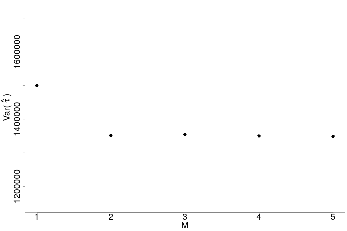
Figure 2: Simulated variances of different experiments.

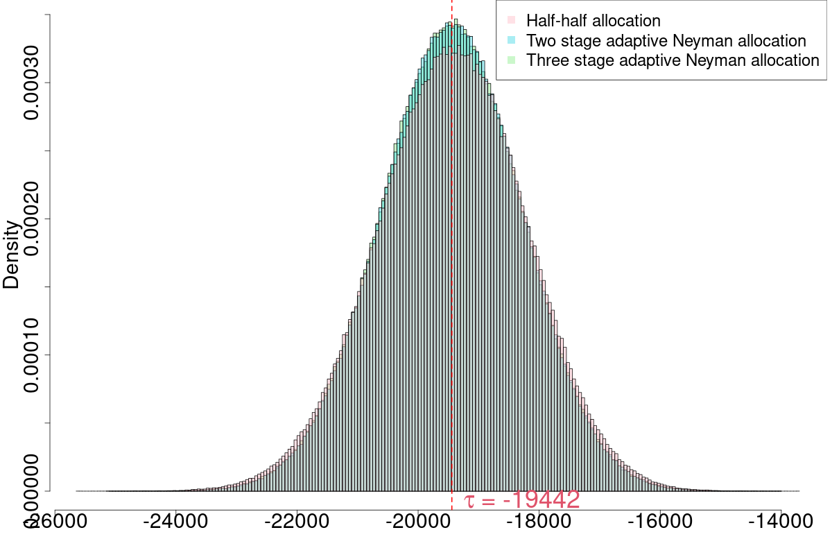
Figure 3: Simulated distributions of different experiments.

For each design, we conduct the experiment and calculate the difference-in-means estimator $\widehat{\tau}$. We compare the variances of the estimators in Figure 2 and compare the distributions of the estimators in Figure 3. Note that, there are two sources of randomness in Figures 2 and 3. First, the resampling process draws random samples when generating the potential outcomes; second, the experiments are randomized experiments when determining the treatment assignments.

In Figure 2, we simulate the variances of the estimator $\widehat{\tau}$. As shown in Figure 2, as $M$ increases, the simulated variance quickly plateaus, and the extra benefit of increasing one more stage becomes smaller and smaller. When $M$ is as small as $2$ or $3$, the numerical performance is already as good as when $M$ takes larger values. In Figure 3 we simulate the distributions of the estimator $\widehat{\tau}$. As shown in Figure 3, all the distributions look unbiased. The two stage and three stage adaptive Neyman allocations have similar performances. Both of them outperform the half-half allocation benchmark.

Our simulations suggest that, on this user click data from a social media site, adaptive Neyman allocation leads to a $\sim 10\%$ reduction in variance compared to half-half allocations. This will lead to faster business decisions as the experimenter would require less samples to draw the same causal conclusion.

8 Conclusions and Limitations

In this paper, we present a competitive analysis framework to study the optimal multi-stage experimental design problem. We propose an adaptive Neyman allocation algorithm that is nearly optimal and almost matches the information-theoretic limit of conducting experiments. Our algorithm allows for efficient allocation of subjects into treated and control groups in multi-stage experiments, and can guide researchers towards the best allocation decisions when standard deviations are unknown in advance. Overall, our approach offers a solution for researchers seeking to optimize their experimental designs and increase statistical power, particularly in cases where the treated and control groups have different standard deviations, such as in social experiments, clinical trials, marketing research, and online A/B testing.

We conclude this paper with two limitations that should serve as cautionary notes for practitioners. First, while adaptive Neyman allocation as described in this paper is suitable for sequential experimental design with a limited sample size, it still requires a minimum amount of sample size, on the scale of at least several hundreds, to have reasonable performance. In cases where a social experiment only involves a very small number of subjects, such as $\sim 30$ districts in a developing economy (Gibson et al. 2023), and especially when there is a constraint that limits the size of the treated group to be only $2$ or $3$, we do not recommend the usage of adaptive Neyman allocation, or any randomized experiment design method. Instead, we recommend conducting non-randomized experiments using the synthetic control method; see, e.g., Abadie and Zhao (2021), Doudchenko et al. (2021).

Second, we have used the proxy mean squared error as the primary objective, instead of using the mean squared error. Since the proxy mean squared error is often not equal to the mean squared error, the confidence intervals derived based on the proxy mean squared error may suffer from coverage issues. In the simulations literature (Asmussen and Glynn 2007, Glasserman 2004, Ross 2013), the bias in the estimated confidence intervals could be fixed if the outcomes are assumed to come from known parametric distribution families. Yet there is no general method that corrects for such a bias. Alternatively, we could borrow ideas from Perchet et al. (2016) and Zhang et al. (2020) to discard earlier stage data and then conduct adaptive Neyman allocation in each new stage to overcome the coverage issue. But since data from earlier stages are discarded, we no longer utilize all the data to estimate the confidence intervals.

Online Appendix

9 Useful Lemmas

9.1 Algebraic Inequalities

Lemma 9.1

Let $G_{1},G_{2}>0$ be positive. Let $g:\mathbb{R}^{+}\to\mathbb{R}^{+}$ be a univariate function defined by

$$g(\rho)=\frac{1}{G_{1}}\frac{\rho^{2}}{(\rho+1)^{2}}+\frac{1}{G_{2}}\frac{1}{(\rho+1)^{2}}.$$

Then,

1. $g(\rho)$ is decreasing when $\rho<\frac{G_{1}}{G_{2}}$, and increasing when $\rho>\frac{G_{1}}{G_{2}}$.

2. $g(\rho)\leq\max\{\frac{1}{G_{1}},\frac{1}{G_{2}}\}$.

Lemma 9.2

Let $\sigma(1),\sigma(0)>0$ be positive. Let $h:\mathbb{R}^{+}\to\mathbb{R}^{+}$ be a univariate function defined by

$$h(\widehat{\rho})=\frac{1}{\widehat{\rho}}\ \sigma^{2}(1)+\widehat{\rho}\ \sigma^{2}(0).$$

Then,

1. $h(\widehat{\rho})$ is decreasing when $\widehat{\rho}<\frac{\sigma(1)}{\sigma(0)}$, and increasing when $\widehat{\rho}>\frac{\sigma(1)}{\sigma(0)}$.

2. $h(\widehat{\rho})$ is a convex function.

3. Let $\zeta\in(0,1)$. When $\frac{\sigma(1)}{\sigma(0)}\sqrt{\frac{1-\zeta}{1+\zeta}}\leq\widehat{\rho}\leq\frac{\sigma(1)}{\sigma(0)}\sqrt{\frac{1+\zeta}{1-\zeta}}$, $h(\widehat{\rho})\leq\sigma(1)\sigma(0)(\sqrt{\frac{1-\zeta}{1+\zeta}}+\sqrt{\frac{1+\zeta}{1-\zeta}})$.

Lemma 9.3

When $T\geq 16$, $\varepsilon\in\left(0,\frac{1}{8}\right)$, the following inequality holds,

$$\left(\frac{T-\frac{1}{2}T^{\frac{1}{2}}}{\frac{1}{2}T^{\frac{1}{2}}}\right)^{4}>\frac{1+2^{\frac{1}{2}}T^{-\frac{1}{4}+\frac{\varepsilon}{2}}}{1-2^{\frac{1}{2}}T^{-\frac{1}{4}+\frac{\varepsilon}{2}}}.$$

Lemma 9.4

Let $M\geq 3$ and $T\geq 16$, and $0<\varepsilon\leq\min\{\frac{1}{M},\frac{1}{100}\}$. For any $m\leq M-1$, let $\beta_{m}=6\cdot 15^{-\frac{m}{M}}$. Then we have, for any $m\leq M-1$,

$$(1-2\beta_{m}^{-1}T^{-\frac{m}{M}+\varepsilon})^{-\frac{1}{2}}\leq 1+2\beta_{m}^{-1}T^{-\frac{m}{M}+\varepsilon}.$$

Lemma 9.5

Let $M\geq 3$, $T\geq 16$, and $0<\varepsilon\leq\min\{\frac{1}{M},\frac{1}{100}\}$. For any $m\leq M-1$, let $\beta_{m}=6\cdot 15^{-\frac{m}{M}}$. Then we have, for any $m\leq M-1$,

$$\sqrt{\frac{1-2^{\frac{1}{2}}\beta_{m}^{-\frac{1}{2}}T^{-\frac{m}{2M}+\frac{\varepsilon}{2}}}{1+2^{\frac{1}{2}}\beta_{m}^{-\frac{1}{2}}T^{-\frac{m}{2M}+\frac{\varepsilon}{2}}}}>\frac{1}{2}.$$

Lemma 9.6

Let $M\geq 3$ and $T\geq 16$. For any $m\leq M-1$, let $\beta_{m}=6\cdot 15^{-\frac{m}{M}}$. Then we have, for any $m\leq M-1$,

$$\frac{T-\frac{1}{2}\beta_{m}T^{\frac{m}{M}}}{\frac{1}{2}\beta_{m}T^{\frac{m}{M}}}\geq 4>2.$$

Lemma 9.7

Let $M\geq 3$ and $T\geq 16$. Let $\beta_{1}=6\cdot 15^{-\frac{1}{M}}$. Then we have

$$\frac{\frac{1}{2}\beta_{1}T^{\frac{1}{M}}}{T-\frac{1}{2}\beta_{1}T^{\frac{1}{M}}}<4\cdot 15^{-\frac{1}{M}}\cdot T^{-\frac{M-1}{M}}.$$

Lemma 9.8

Let $0<\epsilon\leq\frac{1}{6}$. Then,

$$\sqrt{1+\frac{3}{2}\epsilon}\leq 1+\frac{3}{4}\epsilon-\frac{9}{64}\epsilon^{2}<1+\frac{3}{4}\epsilon.$$

Lemma 9.9

Let $0<\epsilon\leq\frac{1}{6}$. Then,

$$\frac{1}{1-\frac{27}{4}\epsilon^{2}-\frac{27}{4}\epsilon^{3}}\leq 1+\frac{27}{2}\epsilon^{2}.$$

9.2 Extensions of Algebraic Inequalities

Lemma 9.10

Let $T\geq 320^{\frac{5}{4}}C^{5}$. Then,

$$T\geq 64C^{4}\log{T}.$$

Lemma 9.11

Let $T\geq(\frac{5000}{3})^{\frac{5}{4}}C^{5}$. Then,

$$T\geq\frac{1000}{3}C^{4}\log{T}.$$

Lemma 9.12

Let $T\geq 320^{\frac{5}{4}}C^{5}$. Then, we have

1. $$4C^{2}T^{-\frac{1}{2}}(\log{T})^{\frac{1}{2}}\leq\frac{1}{2}.$$

2. $$\left(\frac{T-2C^{2}T^{\frac{1}{2}}(\log{T})^{\frac{1}{2}}}{2C^{2}T^{\frac{1}{2}}(\log{T})^{\frac{1}{2}}}\right)^{4}>\frac{1+2CT^{-\frac{1}{4}}(\log{T})^{\frac{1}{4}}}{1-2CT^{-\frac{1}{4}}(\log{T})^{\frac{1}{4}}}.$$

3. $$\left(1-4C^{2}T^{-\frac{1}{2}}(\log{T})^{\frac{1}{2}}\right)^{-\frac{1}{2}}\leq 4C^{2}T^{-\frac{1}{2}}(\log{T})^{\frac{1}{2}}$$

Lemma 9.13

Let $M\geq 3$, $T\geq(\frac{5000}{3})^{\frac{5}{4}}C^{5}$. Let $\beta_{m}=\frac{400}{3}C^{4}\log{T}\cdot(\frac{1000}{3}C^{4}\log{T})^{-\frac{m}{M}}$ for any $m\leq M-1$. Then we have, for any $m\leq M-1$,

$$(1-48C^{4}\beta_{m}^{-1}T^{-\frac{m}{M}}\log{T})^{-\frac{1}{2}}\leq 1+48C^{4}\beta_{m}^{-1}T^{-\frac{m}{M}}\log{T}.$$

Lemma 9.14

Let $M\geq 3$, $T\geq(\frac{5000}{3})^{\frac{5}{4}}C^{5}$. Let $\beta_{m}=\frac{400}{3}C^{4}\log{T}\cdot(\frac{1000}{3}C^{4}\log{T})^{-\frac{m}{M}}$ for any $m\leq M-1$. Then we have, for any $m\leq M-1$,

$$\sqrt{\frac{1-48^{\frac{1}{2}}C^{2}\beta_{m}^{-\frac{1}{2}}T^{-\frac{m}{2M}}(\log{T})^{\frac{1}{2}}}{1+48^{\frac{1}{2}}C^{2}\beta_{m}^{-\frac{1}{2}}T^{-\frac{m}{2M}}(\log{T})^{\frac{1}{2}}}}>\frac{1}{2}.$$

Lemma 9.15

Let $M\geq 3$, $T\geq(\frac{5000}{3})^{\frac{5}{4}}C^{5}$. Let $\beta_{m}=\frac{400}{3}C^{4}\log{T}\cdot(\frac{1000}{3}C^{4}\log{T})^{-\frac{m}{M}}$ for any $m\leq M-1$. Then we have, for any $m\leq M-1$,

$$\frac{T-\frac{1}{2}\beta_{m}T^{\frac{m}{M}}}{\frac{1}{2}\beta_{m}T^{\frac{m}{M}}}\geq 4>2.$$

Lemma 9.16

Let $M\geq 3$, $T\geq(\frac{5000}{3})^{\frac{5}{4}}C^{5}$. Let $\beta_{1}=\frac{400}{3}C^{4}\log{T}\cdot(\frac{1000}{3}C^{4}\log{T})^{-\frac{1}{M}}$. Then we have

$$\frac{\frac{1}{2}\beta_{1}T^{\frac{1}{M}}}{T-\frac{1}{2}\beta_{1}T^{\frac{1}{M}}}<4\cdot 15^{-\frac{1}{M}}C^{\frac{2(M-1)}{M}}\cdot T^{-\frac{M-1}{M}}(\log{T})^{\frac{M-1}{M}}.$$

9.3 Probability Inequalities

Lemma 9.17

Let $Y_{1},...,Y_{n}$ be $n$ identical and independent copies of some random variable $Y$. Let $\sigma^{2}$ be the variance of $Y$, and let $\widehat{\sigma}^{2}=\frac{1}{n-1}\sum_{i=1}^{n}\left(Y_{i}-\frac{1}{n}\sum_{i=1}^{n}Y_{i}\right)^{2}$ be the sample variance estimator. The variance of the sample variance estimator can be expressed as

$$\mathrm{E}\left[\left(\widehat{\sigma}^{2}\right)^{2}\right]=\frac{1}{n}\mathrm{E}\left[(Y-\mathrm{E}Y)^{4}\right]+\frac{n^{2}-2n+3}{n(n-1)}\sigma^{4}.$$

Lemma 9.18

At the end of stage $m$, consider the sample variance estimators as defined in (7a) and (7b). Under Assumption 4, for any $m\in[M]$ and for any $\delta>0$, if $\sum_{l=1}^{m}T_{l}(1)\geq 3$, then

$$\Pr\left(|\widehat{\sigma}^{2}_{m}(1)-\sigma^{2}(1)|\geq\delta\right)\leq \ \frac{\kappa(1)\sigma^{4}(1)}{\delta^{2}\sum_{l=1}^{m}T_{l}(1)}.$$

If $\sum_{l=1}^{m}T_{l}(0)\geq 3$, then

$$\Pr\left(|\widehat{\sigma}^{2}_{m}(0)-\sigma^{2}(0)|\geq\delta\right)\leq \ \frac{\kappa(0)\sigma^{4}(0)}{\delta^{2}\sum_{l=1}^{m}T_{l}(0)},$$

where $\kappa(1)$ and $\kappa(0)$ are defined in Assumption 4.

Lemma 9.19

Consider, either the sample variance estimators as defined in (5a) and (5b) at the end of the first stage, or the sample variance estimators as defined in (7a) and (7b) at the end of stage $m$. Under Assumption 6, for any $m\leq M-1$ and for any $\delta>0$,

$$\Pr\left(|\widehat{\sigma}^{2}_{m}(1)-\sigma^{2}(1)|\geq\delta\right)\leq \ 2\exp\left\{-\frac{\delta^{2}\sum_{l=1}^{m}T_{l}(1)}{8C^{4}\sigma^{4}(1)}\right\},$$

$$\Pr\left(|\widehat{\sigma}^{2}_{m}(0)-\sigma^{2}(0)|\geq\delta\right)\leq \ 2\exp\left\{-\frac{\delta^{2}\sum_{l=1}^{m}T_{l}(0)}{8C^{4}\sigma^{4}(0)}\right\},$$

where $C$ is defined in Assumption 6.

10 Missing Proofs

10.1 Proofs of Lemmas from Section 9

10.1.1 Proof of Lemma 9.1

Proof 10.1

Proof of Lemma 9.1. Taking first order derivative, we have

$$g^{\prime}(\rho)= \ \frac{1}{G_{1}}\cdot\frac{2\rho}{(\rho+1)^{3}}-\frac{1}{G_{2}}\cdot\frac{2}{(\rho+1)^{3}}$$

$$= \ \frac{2}{(\rho+1)^{3}}\left(\frac{\rho}{G_{1}}-\frac{1}{G_{2}}\right).$$

When $\rho<\frac{G_{1}}{G_{2}}$, $g^{\prime}(\rho)<0$ so $g(\rho)$ is decreasing; when $\rho>\frac{G_{1}}{G_{2}}$, $g^{\prime}(\rho)>0$ so $g(\rho)$ is increasing.

Using the above, we have that

$$g(\rho)\leq\max\left\{\lim_{\rho\to+\infty}g(\rho),\lim_{\rho\to 0^{+}}g(\rho)\right\}=\max\left\{\frac{1}{G_{1}},\frac{1}{G_{2}}\right\}.$$

10.1.2 Proof of Lemma 9.2

Proof 10.2

Proof of Lemma 9.2. Taking first order derivative, we have

$$h^{\prime}(\widehat{\rho})=\sigma^{2}(0)-\frac{1}{\widehat{\rho}^{2}}\ \sigma^{2}(1).$$

When $\widehat{\rho}<\frac{\sigma(1)}{\sigma(0)}$, $h^{\prime}(\widehat{\rho})<0$, so $h(\widehat{\rho})$ is decreasing in $\widehat{\rho}$; when $\widehat{\rho}>\frac{\sigma(1)}{\sigma(0)}$, $h^{\prime}(\widehat{\rho})>0$, so $h(\widehat{\rho})$ is increasing in $\widehat{\rho}$.

Next, taking second order derivative, we have

$$h^{\prime}(\widehat{\rho})=\frac{2}{\widehat{\rho}^{3}}\ \sigma^{2}(1)>0.$$

So $h(\widehat{\rho})$ is a convex function.

Combing above, we know that $h(\widehat{\rho})$ is a convex function, increasing when $\widehat{\rho}>\frac{\sigma(1)}{\sigma(0)}$ and decreasing when $\widehat{\rho}<\frac{\sigma(1)}{\sigma(0)}$. When $\frac{\sigma(1)}{\sigma(0)}\sqrt{\frac{1-\zeta}{1+\zeta}}\leq\widehat{\rho}\leq\frac{\sigma(1)}{\sigma(0)}\sqrt{\frac{1+\zeta}{1-\zeta}}$, the maximum is taken on the boundaries, i.e.,

$$h(\widehat{\rho})\leq\max\left\{h\left(\frac{\sigma(1)}{\sigma(0)}\sqrt{\frac{1-\zeta}{1+\zeta}}\right),h\left(\frac{\sigma(1)}{\sigma(0)}\sqrt{\frac{1+\zeta}{1-\zeta}}\right)\right\}=\sigma(1)\sigma(0)\left(\sqrt{\frac{1-\zeta}{1+\zeta}}+\sqrt{\frac{1+\zeta}{1-\zeta}}\right).$$

10.1.3 Proof of Lemma 9.3

Proof 10.3

Proof of Lemma 9.3. When $T\geq 16$, we have

$$\frac{T-\frac{1}{2}T^{\frac{1}{2}}}{\frac{1}{2}T^{\frac{1}{2}}}>3>\left(\frac{1+2^{-\frac{1}{4}}}{1-2^{-\frac{1}{4}}}\right)^{4}\approx 1.84.$$ (9)

On the other hand, when $T\geq 16$ and $\varepsilon\in\left(0,\frac{1}{8}\right)$, we have $T^{1-2\varepsilon}\geq 8=\left(2^{\frac{3}{4}}\right)^{4}$, which then suggests $2^{-\frac{1}{2}}T^{\frac{1}{4}-\frac{\varepsilon}{2}}\geq 2^{\frac{1}{4}}>0$. So

$$0<2^{\frac{1}{2}}T^{-\frac{1}{4}+\frac{\varepsilon}{2}}\leq 2^{-\frac{1}{4}}.$$

Since $\frac{1+x}{1-x}$ is an increasing function on $x>0$, we have

$$\frac{1+2^{-\frac{1}{4}}}{1-2^{-\frac{1}{4}}}\geq\frac{1+2^{\frac{1}{2}}T^{-\frac{1}{4}+\frac{\varepsilon}{2}}}{1-2^{\frac{1}{2}}T^{-\frac{1}{4}+\frac{\varepsilon}{2}}}.$$ (10)

Combining (9) and (10) we finish the proof.

10.1.4 Proof of Lemma 9.4

Proof 10.4

Proof of Lemma 9.4. When $0\leq x\leq\frac{1}{2}$, we have $x+x^{2}\leq 1$. Then, since $x\geq 0$, we have $1\leq 1+x-x^{2}-x^{3}=(1+x)^{2}(1-x)$. Since $1-x>0$, this leads to $0<\frac{1}{1-x}\leq(1+x)^{2}$. Taking square root we have

$$(1-x)^{-\frac{1}{2}}\leq 1+x.$$ (11)

Next we show that $\beta_{m}^{-1}T^{-\frac{m}{M}+\varepsilon}\leq\frac{1}{4}$. To see this, we use the definition of $\beta_{m}=6\cdot 15^{-\frac{m}{M}}$.

$$\beta_{m}^{-1}T^{-\frac{m}{M}+\varepsilon}=\frac{1}{6}\cdot\left(\frac{1}{15}\right)^{-\frac{m}{M}}T^{-\frac{m}{M}+\varepsilon}=\frac{15^{\varepsilon}}{6}\cdot\left(\frac{T}{15}\right)^{-\frac{m}{M}+\varepsilon}\leq\frac{15^{\varepsilon}}{6}\leq\frac{15^{\frac{1}{100}}}{6}\approx 0.1713<\frac{1}{4}.$$

where the first inequality is because $T>15$ and $-\frac{m}{M}+\varepsilon\leq 0$; the second inequality is because $0<\varepsilon\leq\frac{1}{100}$. Replacing $x=2\beta_{m}^{-1}T^{-\frac{m}{M}+\varepsilon}$ into (11) we finish the proof.

10.1.5 Proof of Lemma 9.5

Proof 10.5

Proof of Lemma 9.5. First we focus on $\beta_{m}^{-1}T^{-\frac{m}{M}+\varepsilon}$. Using the definition of $\beta_{m}=6\cdot 15^{-\frac{m}{M}}$,

$$\beta_{m}^{-1}T^{-\frac{m}{M}+\varepsilon}=\frac{1}{6}\cdot\left(\frac{1}{15}\right)^{-\frac{m}{M}}T^{-\frac{m}{M}+\varepsilon}=\frac{15^{\varepsilon}}{6}\cdot\left(\frac{T}{15}\right)^{-\frac{m}{M}+\varepsilon}\leq\frac{15^{\varepsilon}}{6}\leq\frac{15^{\frac{1}{100}}}{6}\approx 0.1713<\frac{9}{50}.$$ (12)

where the first inequality is because $T>15$ and $-\frac{m}{M}+\varepsilon\leq 0$; the second inequality is because $0<\varepsilon\leq\frac{1}{100}$.

Using (12) as above, we have

$$0<2^{\frac{1}{2}}\beta_{m}^{-\frac{1}{2}}T^{-\frac{m}{2M}+\frac{\varepsilon}{2}}<\frac{3}{5}<1.$$

Since $\frac{1-x}{1+x}$ is a decreasing function in $x$ when $0<x<1$,

$$\frac{1-2^{\frac{1}{2}}\beta_{m}^{-\frac{1}{2}}T^{-\frac{m}{2M}+\frac{\varepsilon}{2}}}{1+2^{\frac{1}{2}}\beta_{m}^{-\frac{1}{2}}T^{-\frac{m}{2M}+\frac{\varepsilon}{2}}}>\frac{1-\frac{3}{5}}{1+\frac{3}{5}}=\frac{1}{4}.$$

Taking square root finishes the proof.

10.1.6 Proof of Lemma 9.6

Proof 10.6

Proof of Lemma 9.6. Using the definition of $\beta_{m}=6\cdot 15^{-\frac{m}{M}}$,

$$0<\frac{5}{2}\beta_{m}T^{\frac{m}{M}}=15\cdot\left(\frac{T}{15}\right)^{\frac{m}{M}}\leq 15\cdot\left(\frac{T}{15}\right)=T,$$

where the inequality is due to $m<M$. Then we have

$$\frac{T-\frac{1}{2}\beta_{m}T^{\frac{m}{M}}}{\frac{1}{2}\beta_{m}T^{\frac{m}{M}}}>\frac{\frac{5}{2}\beta_{m}T^{\frac{m}{M}}-\frac{1}{2}\beta_{m}T^{\frac{m}{M}}}{\frac{1}{2}\beta_{m}T^{\frac{m}{M}}}=4,$$

which finishes the proof.

10.1.7 Proof of Lemma 9.7

Proof 10.7

Proof of Lemma 9.7. Using the definition of $\beta_{1}=6\cdot 15^{-\frac{1}{M}}$,

$$\frac{1}{4}T=\left(\frac{1}{2}\beta_{1}T^{\frac{1}{M}}\right)\cdot\left(\frac{1}{12}15^{\frac{1}{M}}T^{\frac{M-1}{M}}\right)>\left(\frac{1}{2}\beta_{1}T^{\frac{1}{M}}\right)\cdot\left(\frac{1}{12}15^{\frac{1}{M}}15^{\frac{M-1}{M}}\right)>\frac{1}{2}\beta_{1}T^{\frac{1}{M}}.$$

Then, replacing $\frac{1}{2}\beta_{1}T^{\frac{1}{M}}$ with $\frac{1}{4}T$ in the denominator, we have

$$\frac{\frac{1}{2}\beta_{1}T^{\frac{1}{M}}}{T-\frac{1}{2}\beta_{1}T^{\frac{1}{M}}}<\frac{\frac{1}{2}\beta_{1}T^{\frac{1}{M}}}{\frac{3}{4}T}=\frac{2}{3}\beta_{1}T^{-\frac{M-1}{M}}=4\cdot 15^{-\frac{1}{M}}\cdot T^{-\frac{M-1}{M}}.$$

10.1.8 Proof of Lemma 9.8

Proof 10.8

Proof of Lemma 9.8. From $\epsilon<1$, we have

$$\frac{3}{4}\epsilon-\frac{9}{128}\epsilon^{2}<\frac{3}{4}\epsilon<1.$$

Since $\epsilon>0$,

$$\frac{27}{128}\epsilon^{3}<\frac{9}{32}\epsilon^{2}+\frac{81}{4096}\epsilon^{4}.$$

Then we have,

$$0<1+\frac{3}{2}\epsilon\leq 1+\frac{3}{2}\epsilon+\frac{9}{16}\epsilon^{2}-\frac{9}{32}\epsilon^{2}-\frac{27}{128}\epsilon^{3}+\frac{81}{4096}\epsilon^{4}=\left(1+\frac{2}{4}\epsilon-\frac{9}{64}\epsilon^{2}\right)^{2}.$$

Taking square root we finish the proof.

10.1.9 Proof of Lemma 9.9

Proof 10.9

Proof of Lemma 9.9. From $\epsilon<\frac{1}{6}$, we have

$$\epsilon+\frac{27}{2}\epsilon^{2}+\frac{27}{2}\epsilon^{3}\leq\frac{1}{6}+\frac{27}{72}+\frac{27}{432}<1.$$

Since $\epsilon>0$,

$$\frac{27}{4}\cdot(\epsilon^{3}+\frac{27}{2}\epsilon^{4}+\frac{27}{2}\epsilon^{5})<\frac{27}{4}\epsilon^{2}.$$

Then we have,

$$1\leq 1-\frac{27}{4}\epsilon^{2}-\frac{27}{4}\epsilon^{3}+\frac{27}{2}\epsilon^{2}-\frac{27^{2}}{8}\epsilon^{4}-\frac{27^{2}}{8}\epsilon^{5}=(1+\frac{27}{2}\epsilon^{2})\cdot\left(1-\frac{27}{4}\epsilon^{2}-\frac{27}{4}\epsilon^{3}\right).$$

Since $1-\frac{27}{4}\epsilon^{2}-\frac{27}{4}\epsilon^{3}>0$, moving it to the left hand side finishes the proof.

10.1.10 Proof of Lemma 9.10

Proof 10.10

Proof of Lemma 9.10. To prove the first claim, note that $\frac{T}{\log{T}}$ is an increasing function, and that $T\geq 320^{\frac{5}{4}}C^{5}$, so we have

$$\frac{T}{64C^{4}\log{T}}>\frac{320^{\frac{5}{4}}C^{5}}{64C^{4}\log{(320^{\frac{5}{4}}C^{5})}}=\frac{320^{\frac{5}{4}}C^{5}}{64C^{4}\cdot 5\cdot\log{(320^{\frac{1}{4}}C)}}=\frac{320^{\frac{1}{4}}C}{\log{(320^{\frac{1}{4}}C)}}\geq 1,$$

which finishes the proof.

10.1.11 Proof of Lemma 9.11

Proof 10.11

Proof of Lemma 9.11. Note that $\frac{T}{\log{T}}$ is an increasing function, and that $T\geq(\frac{5000}{3})^{\frac{5}{4}}C^{5}$, so we have

$$\frac{T}{\frac{1000}{3}C^{4}\log{T}}>\frac{(\frac{5000}{3})^{\frac{5}{4}}C^{5}}{\frac{1000}{3}C^{4}\log{((\frac{5000}{3})^{\frac{5}{4}}C^{5})}}=\frac{(\frac{5000}{3})^{\frac{5}{4}}C^{5}}{\frac{1000}{3}C^{4}\cdot 5\cdot\log{((\frac{5000}{3})^{\frac{1}{4}}C)}}=\frac{(\frac{5000}{3})^{\frac{1}{4}}C}{\log{((\frac{5000}{3})^{\frac{1}{4}}C)}}\geq 1,$$

which finishes the proof.

10.1.12 Proof of Lemma 9.12

Proof 10.12

Proof of Lemma 9.12. To prove the first claim, we re-arrange terms from Lemma 9.10 and obtain

$$4C^{2}T^{-\frac{1}{2}}(\log{T})^{\frac{1}{2}}\leq\frac{1}{2}.$$

To prove the second claim, note that from above, we have $T\geq 8C^{2}T^{\frac{1}{2}}(\log{T})^{\frac{1}{2}}$, so that

$$\left(\frac{T-2C^{2}T^{\frac{1}{2}}(\log{T})^{\frac{1}{2}}}{2C^{2}T^{\frac{1}{2}}(\log{T})^{\frac{1}{2}}}\right)^{4}\geq 3^{4}$$

We also have $2CT^{-\frac{1}{4}}(\log{T})^{\frac{1}{4}}\leq\frac{\sqrt{2}}{2}$, so that

$$\frac{1+2CT^{-\frac{1}{4}}(\log{T})^{\frac{1}{4}}}{1-2CT^{-\frac{1}{4}}(\log{T})^{\frac{1}{4}}}\leq\frac{1+\frac{\sqrt{2}}{2}}{1-\frac{\sqrt{2}}{2}}<3^{4},$$

which concludes the proof of the second claim.

To prove the third claim, note that when $0\leq x\leq\frac{1}{2}$, we have $x+x^{2}\leq 1$. Then, since $x\geq 0$, we have $1\leq 1+x-x^{2}-x^{3}=(1+x)^{2}(1-x)$. Since $1-x>0$, this leads to $0<\frac{1}{1-x}\leq(1+x)^{2}$. Taking square root we have

$$(1-x)^{-\frac{1}{2}}\leq 1+x.$$

Replacing $x=4C^{2}T^{-\frac{1}{2}}(\log{T})^{\frac{1}{2}}$ we conclude the proof of the third claim.

10.1.13 Proof of Lemma 9.13

Proof 10.13

Proof of Lemma 9.13. When $0\leq x\leq\frac{1}{2}$, we have $x+x^{2}\leq 1$. Then, since $x\geq 0$, we have $1\leq 1+x-x^{2}-x^{3}=(1+x)^{2}(1-x)$. Since $1-x>0$, this leads to $0<\frac{1}{1-x}\leq(1+x)^{2}$. Taking square root we have

$$(1-x)^{-\frac{1}{2}}\leq 1+x.$$

Using the definition of $\beta_{m}=\frac{400}{3}C^{4}\log{T}\cdot(\frac{1000}{3}C^{4}\log{T})^{-\frac{m}{M}}$,

$$48C^{4}\beta_{m}^{-1}T^{-\frac{m}{M}}\log{T}=\frac{9}{25}\left(\frac{T}{\frac{1000}{3}C^{4}\log{T}}\right)^{-\frac{m}{M}}\leq\frac{9}{25}<\frac{1}{2},$$

where the first inequality is due to Lemma 9.11 and $m\geq 1$.

Replacing $x=48C^{4}\beta_{m}^{-1}T^{-\frac{m}{M}}\log{T}$ finishes the proof.

10.1.14 Proof of Lemma 9.14

Proof 10.14

Proof of Lemma 9.14. Using the definition of $\beta_{m}=\frac{400}{3}C^{4}\log{T}\cdot(\frac{1000}{3}C^{4}\log{T})^{-\frac{m}{M}}$,

$$48C^{4}\beta_{m}^{-1}T^{-\frac{m}{M}}\log{T}=\frac{9}{25}\left(\frac{T}{\frac{1000}{3}C^{4}\log{T}}\right)^{-\frac{m}{M}}\leq\frac{9}{25},$$ (13)

where the first inequality is due to Lemma 9.11 and $m\geq 1$.

Using (13) as above, we have

$$0<48^{\frac{1}{2}}C^{2}\beta_{m}^{-\frac{1}{2}}T^{-\frac{m}{2M}}(\log{T})^{\frac{1}{2}}<\frac{3}{5}<1.$$

Since $\frac{1-x}{1+x}$ is a decreasing function in $x$ when $0<x<1$,

$$\frac{1-48^{\frac{1}{2}}C^{2}\beta_{m}^{-\frac{1}{2}}T^{-\frac{m}{2M}}(\log{T})^{\frac{1}{2}}}{1+48^{\frac{1}{2}}C^{2}\beta_{m}^{-\frac{1}{2}}T^{-\frac{m}{2M}}(\log{T})^{\frac{1}{2}}}>\frac{1-\frac{3}{5}}{1+\frac{3}{5}}=\frac{1}{4}.$$

Taking square root finishes the proof.

10.1.15 Proof of Lemma 9.15

Proof 10.15

Proof of Lemma 9.15. Using the definition of $\beta_{m}=\frac{400}{3}C^{4}\log{T}\cdot(\frac{1000}{3}C^{4}\log{T})^{-\frac{m}{M}}$,

$$0<\frac{5}{2}\beta_{m}T^{\frac{m}{M}}=\frac{1000}{3}C^{4}\log{T}\cdot\left(\frac{T}{\frac{1000}{3}C^{4}\log{T}}\right)^{\frac{m}{M}}<\frac{1000}{3}C^{4}\log{T}\cdot\left(\frac{T}{\frac{1000}{3}C^{4}\log{T}}\right)=T,$$

where the inequality is due to Lemma 9.11 and $m<M$. Then we have

$$\frac{T-\frac{1}{2}\beta_{m}T^{\frac{m}{M}}}{\frac{1}{2}\beta_{m}T^{\frac{m}{M}}}>\frac{\frac{5}{2}\beta_{m}T^{\frac{m}{M}}-\frac{1}{2}\beta_{m}T^{\frac{m}{M}}}{\frac{1}{2}\beta_{m}T^{\frac{m}{M}}}=4,$$

which finishes the proof.

10.1.16 Proof of Lemma 9.16

Proof 10.16

Proof of Lemma 9.16. Using the definition of $\beta_{1}=\frac{400}{3}C^{4}\log{T}\cdot(\frac{1000}{3}C^{4}\log{T})^{-\frac{1}{M}}$,

$$\frac{1}{2}\beta_{1}T^{\frac{1}{M}}=\frac{200}{3}C^{4}\log{T}\cdot\left(\frac{T}{\frac{1000}{3}C^{4}\log{T}}\right)^{\frac{1}{M}}\leq\frac{200}{3}C^{4}\log{T}\cdot\left(\frac{T}{\frac{1000}{3}C^{4}\log{T}}\right)=\frac{1}{5}T,$$

where the inequality is due to Lemma 9.11. Then, replacing $\frac{1}{2}\beta_{1}T^{\frac{1}{M}}$ with $\frac{1}{5}T$ in the denominator, we have

$$\frac{\frac{1}{2}\beta_{1}T^{\frac{1}{M}}}{T-\frac{1}{2}\beta_{1}T^{\frac{1}{M}}}<\frac{\frac{1}{2}\beta_{1}T^{\frac{1}{M}}}{\frac{4}{5}T}=\frac{250}{3}C^{4}\log{T}\cdot\left(\frac{T}{\frac{1000}{3}C^{4}\log{T}}\right)^{\frac{1}{M}}\cdot T^{-1}\\ =96\cdot\left(\frac{1000}{3}\right)^{-\frac{1}{M}}C^{\frac{4(M-1)}{M}}\cdot T^{-\frac{M-1}{M}}(\log{T})^{\frac{M-1}{M}},$$

where the last inequality is re-arranging terms, and using the fact that $\frac{250}{3}<96$.

10.1.17 Proof of Lemma 9.17

Proof 10.17

Proof of Lemma 9.17. Note that we can re-write the sample variance estimator as

$$\widehat{\sigma}^{2}=\frac{1}{n(n-1)}\left(n\cdot\sum_{i=1}^{n}Y_{i}^{2}-(\sum_{i=1}^{n}Y_{i})^{2}\right).$$

We now expand the variance of the sample variance estimator.

$$(\widehat{\sigma}^{2})^{2}=\frac{1}{n^{2}(n-1)^{2}}\left(n^{2}(\sum_{i=1}^{n}Y_{i}^{2})^{2}-2n(\sum_{i=1}^{n}Y_{i}^{2})(\sum_{i=1}^{n}Y_{i})^{2}+(\sum_{i=1}^{n}Y_{i})^{4}\right)$$

Note that, the first term after taking expectation is

$$\mathrm{E}\left[(\sum_{i=1}^{n}Y_{i}^{2})^{2}\right]=n\mathrm{E}\left[Y^{4}\right]+n(n-1)(\mathrm{E}[Y^{2}])^{2}.$$

The second term is

$$\mathrm{E}\left[(\sum_{i=1}^{n}Y_{i}^{2})(\sum_{i=1}^{n}Y_{i})^{2}\right]=n\mathrm{E}\left[Y^{4}\right]+n(n-1)(\mathrm{E}[Y^{2}])^{2}+2n(n-1)\mathrm{E}\left[Y^{3}\right]\mathrm{E}[Y]\\ +n(n-1)(n-2)\mathrm{E}\left[Y^{2}\right](\mathrm{E}[Y])^{2}.$$

The third term is

$$\mathrm{E}\left[(\sum_{i=1}^{n}Y_{i})^{4}\right]=n\mathrm{E}\left[Y^{4}\right]+3n(n-1)(\mathrm{E}[Y^{2}])^{2}+4n(n-1)\mathrm{E}\left[Y^{3}\right]\mathrm{E}[Y]\\ +6n(n-1)(n-2)\mathrm{E}\left[Y^{2}\right](\mathrm{E}[Y])^{2}+n(n-1)(n-2)(n-3)(\mathrm{E}[Y])^{4}.$$

Due to linearity of expectations and merging common terms,

$$\mathrm{E}\left[(\widehat{\sigma}^{2})^{2}\right]=\frac{1}{n^{2}(n-1)^{2}}\Bigg{(}n(n-1)^{2}\mathrm{E}\left[Y^{4}\right]-4n(n-1)^{2}\mathrm{E}\left[Y^{3}\right]\mathrm{E}[Y]+n(n-1)(n^{2}-2n+3)(\mathrm{E}[Y^{2}])^{2}\\ -2n(n-1)(n-2)(n-3)\mathrm{E}\left[Y^{2}\right](\mathrm{E}[Y])^{2}+n(n-1)(n-2)(n-3)(\mathrm{E}[Y])^{4}\Bigg{)}$$ (14)

Note that,

$$\mathrm{E}\left[(Y-\mathrm{E}[Y])^{4}\right]=\ \mathrm{E}\left[Y^{4}\right]-4\mathrm{E}\left[Y^{3}\right]\mathrm{E}[Y]+6\left[Y^{2}\right](\mathrm{E}[Y])^{2}-3\left(\mathrm{E}[Y]\right)^{4},$$

and

$$\left(\mathrm{E}\left[(Y-\mathrm{E}[Y])^{2}\right]\right)^{2}:=\sigma^{4}=\ \mathrm{E}\left[Y^{2}\right]^{2}-\mathrm{E}\left[Y^{2}\right](\mathrm{E}[Y])^{2}+\left(\mathrm{E}[Y]\right)^{4}.$$

Putting the above two expressions into (14) we have

$$\mathrm{E}\left[(\widehat{\sigma}^{2})^{2}\right]= \ \frac{1}{n^{2}(n-1)^{2}}\Bigg{(}n(n-1)^{2}\mathrm{E}\left[(Y-\mathrm{E}[Y])^{4}\right]+n(n-1)(n^{2}-2n+3)\left(\mathrm{E}\left[(Y-\mathrm{E}[Y])^{2}\right]\right)^{2}\Bigg{)}$$

$$= \ \frac{1}{n}\mathrm{E}\left[(Y-\mathrm{E}[Y])^{4}\right]+\frac{n^{2}-2n+3}{n(n-1)}\sigma^{4}$$

which finishes the proof.

10.1.18 Proof of Lemma 9.18

Proof 10.18

Proof of Lemma 9.18. We prove the first inequality, and the second follows similarly.

Due to Chebyshev inequality,

$$\Pr\left(|\widehat{\sigma}^{2}_{m}(1)-\sigma^{2}(1)|\geq\delta\right)\leq\frac{\mathrm{E}\left[(\widehat{\sigma}^{2}_{m}(1)-\sigma^{2}(1))^{2}\right]}{\delta^{2}}.$$ (15)

Note that,

$$\mathrm{E}\left[(\widehat{\sigma}^{2}_{m}(1)-\sigma^{2}(1))^{2}\right]= \ \mathrm{E}\left[(\widehat{\sigma}^{2}_{m}(1))^{2}\right]-\mathrm{E}[\sigma^{4}(1)].$$

Using Lemma 9.17, the above can be expressed as

$$\mathrm{E}\left[(\widehat{\sigma}^{2}_{m}(1)-\sigma^{2}(1))^{2}\right]= \ \frac{1}{\sum_{l=1}^{m}T_{l}(1)}\kappa(1)\sigma^{4}(1)-\frac{\sum_{l=1}^{m}T_{l}(1)-3}{(\sum_{l=1}^{m}T_{l}(1))(\sum_{l=1}^{m}T_{l}(1)-1)}\sigma^{4}(1)$$

$$= \ \frac{\kappa(1)-1}{\sum_{l=1}^{m}T_{l}(1)}\sigma^{4}(1)+\frac{2}{(\sum_{l=1}^{m}T_{l}(1))(\sum_{l=1}^{m}T_{l}(1)-1)}\sigma^{4}(1)$$

$$\leq \ \frac{\kappa(1)-1}{\sum_{l=1}^{m}T_{l}(1)}\sigma^{4}(1)+\frac{3}{(\sum_{l=1}^{m}T_{l}(1))^{2}}\sigma^{4}(1)$$

$$\leq \ \frac{\kappa(1)}{\sum_{l=1}^{m}T_{l}(1)}\sigma^{4}(1),$$

where the last two inequalities are due to $\sum_{l=1}^{m}T_{l}(1)\geq 3$. Putting this inequality back to (15) we finish the proof.

10.1.19 Proof of Lemma 9.19

Proof 10.19

Proof of Lemma 9.19. The proof is by applying the bounded difference inequality.

First, denote $N=\sum_{l=1}^{m}T_{l}(1)$ as a short-hand notion. Denote $\phi(Y_{1},...,Y_{N})=\widehat{\sigma}^{2}_{m}(1)$ to emphasize the dependence on all the potential outcomes up to $N$. Conditional on $W_{1},...,W_{N}$, we distinguish between two cases. If $W_{i}=0$, then

$$\phi(Y_{1},...,Y_{i},...,Y_{N})-\phi(Y_{1},...,Y^{\prime}_{i},...,Y_{N})=0.$$

If $W_{i}=1$, then

$$\phi(Y_{1},...,Y_{i},...,Y_{N})-\phi(Y_{1},...,Y^{\prime}_{i},...,Y_{N})$$

$$= \ \frac{1}{N-1}\sum_{\begin{subarray}{c}t:W_{t}=1\\ t\neq i\end{subarray}}\bigg{(}Y_{t}-\frac{1}{N}\sum_{\begin{subarray}{c}t^{\prime}:W_{t^{\prime}}=1\\ t^{\prime}\neq i\end{subarray}}Y_{t^{\prime}}-\frac{1}{N}Y_{i}\bigg{)}^{2}+\frac{1}{N-1}\bigg{(}Y_{i}-\frac{1}{N}\sum_{\begin{subarray}{c}t^{\prime}:W_{t^{\prime}}=1\\ t^{\prime}\neq i\end{subarray}}Y_{t^{\prime}}-\frac{1}{N}Y_{i}\bigg{)}^{2}$$

$$\quad-\frac{1}{N-1}\sum_{\begin{subarray}{c}t:W_{t}=1\\ t\neq i\end{subarray}}\bigg{(}Y_{t}-\frac{1}{N}\sum_{\begin{subarray}{c}t^{\prime}:W_{t^{\prime}}=1\\ t^{\prime}\neq i\end{subarray}}Y_{t^{\prime}}-\frac{1}{N}Y^{\prime}_{i}\bigg{)}^{2}-\frac{1}{N-1}\bigg{(}Y^{\prime}_{i}-\frac{1}{N}\sum_{\begin{subarray}{c}t^{\prime}:W_{t^{\prime}}=1\\ t^{\prime}\neq i\end{subarray}}Y_{t^{\prime}}-\frac{1}{N}Y^{\prime}_{i}\bigg{)}^{2}$$

$$= \ \frac{1}{N-1}\sum_{\begin{subarray}{c}t:W_{t}=1\\ t\neq i\end{subarray}}\bigg{\{}\frac{2}{N}\bigg{(}Y_{t}-\frac{1}{N}\sum_{\begin{subarray}{c}t^{\prime}:W_{t^{\prime}}=1\\ t^{\prime}\neq i\end{subarray}}Y_{t^{\prime}}\bigg{)}\left(Y^{\prime}_{i}-Y_{i}\right)+\frac{1}{N^{2}}\left(Y_{i}^{2}-(Y^{\prime}_{i})^{2}\right)\bigg{\}}$$ (16)

$$\quad+\frac{1}{N-1}\bigg{\{}\bigg{(}\frac{N-1}{N}Y_{i}-\frac{1}{N}\sum_{\begin{subarray}{c}t^{\prime}:W_{t^{\prime}}=1\\ t^{\prime}\neq i\end{subarray}}Y_{t^{\prime}}\bigg{)}^{2}-\bigg{(}\frac{N-1}{N}Y^{\prime}_{i}-\frac{1}{N}\sum_{\begin{subarray}{c}t^{\prime}:W_{t^{\prime}}=1\\ t^{\prime}\neq i\end{subarray}}Y_{t^{\prime}}\bigg{)}^{2}\bigg{\}}.$$ (17)

To start with (16), we see that it is equal to

$$\ \frac{1}{N-1}\sum_{\begin{subarray}{c}t:W_{t}=1\\ t\neq i\end{subarray}}\frac{2}{N}(Y^{\prime}_{i}-Y_{i})\bigg{(}Y_{t}-\frac{1}{N}\sum_{\begin{subarray}{c}t^{\prime}:W_{t^{\prime}}=1\\ t^{\prime}\neq i\end{subarray}}Y_{t^{\prime}}\bigg{)}+\frac{1}{N-1}\frac{N-1}{N^{2}}\left(Y_{i}^{2}-(Y^{\prime}_{i})^{2}\right)$$

$$= \ \frac{2}{N(N-1)}(Y^{\prime}_{i}-Y_{i})\bigg{(}\sum_{\begin{subarray}{c}t:W_{t}=1\\ t\neq i\end{subarray}}Y_{t}-\frac{N-1}{N}\sum_{\begin{subarray}{c}t^{\prime}:W_{t^{\prime}}=1\\ t^{\prime}\neq i\end{subarray}}Y_{t^{\prime}}\bigg{)}+\frac{1}{N^{2}}\left(Y_{i}^{2}-(Y^{\prime}_{i})^{2}\right)$$

$$= \ \frac{2}{N^{2}(N-1)}(Y^{\prime}_{i}-Y_{i})\sum_{\begin{subarray}{c}t:W_{t}=1\\ t\neq i\end{subarray}}Y_{t}+\frac{1}{N^{2}}\left(Y_{i}^{2}-(Y^{\prime}_{i})^{2}\right).$$

Next, focusing on (17), we see that it is equal to

$$\ \frac{1}{N-1}\bigg{\{}\frac{(N-1)^{2}}{N^{2}}\left(Y_{i}^{2}-(Y^{\prime}_{i})^{2}\right)+2\frac{N-1}{N}\frac{1}{N}(Y^{\prime}_{i}-Y_{i})\sum_{\begin{subarray}{c}t^{\prime}:W_{t^{\prime}}=1\\ t^{\prime}\neq i\end{subarray}}Y_{t^{\prime}}\bigg{\}}$$

$$= \ \frac{N-1}{N^{2}}\left(Y_{i}^{2}-(Y^{\prime}_{i})^{2}\right)+\frac{2}{N^{2}}(Y^{\prime}_{i}-Y_{i})\sum_{\begin{subarray}{c}t:W_{t}=1\\ t\neq i\end{subarray}}Y_{t}.$$

Combining both parts, we have

$$|\phi(Y_{1},...,Y_{i},...,Y_{N})-\phi(Y_{1},...,Y^{\prime}_{i},...,Y_{N})|= \ \bigg{|}\frac{1}{N}\left(Y_{i}^{2}-(Y^{\prime}_{i})^{2}\right)+\frac{2}{N(N-1)}(Y^{\prime}_{i}-Y_{i})\sum_{\begin{subarray}{c}t:W_{t}=1\\ t\neq i\end{subarray}}Y_{t}\bigg{|}$$

$$= \ \frac{1}{N}\bigg{|}(Y^{\prime}_{i}-Y_{i})\bigg{(}\frac{2}{N-1}\sum_{\begin{subarray}{c}t:W_{t}=1\\ t\neq i\end{subarray}}Y_{t}-(Y^{\prime}_{i}+Y_{i})\bigg{)}\bigg{|}.$$

Note that for any $x,y,z\in[-V,V]$, we have

$$|(x-y)(2z-(x+y))|\leq \ \max\left\{|(x-y)(2V-(x+y))|,|(x-y)(-2V-(x+y))|\right\}$$

$$= \ \max\left\{|2(x-y)V-(x^{2}-y^{2})|,|2(x-y)V+(x^{2}-y^{2})|\right\}$$

$$\leq \ 4V^{2},$$

where the first inequality is because the function is monotone with respect to $z$; the last inequality is because both functions are monotone with respect to $x$ and $y$. Replacing $x=Y^{\prime}_{i}$, $y=Y_{i}$, $z=\frac{1}{N-1}\sum_{\begin{subarray}{c}t:W_{t}=1\\ t\neq i\end{subarray}}Y_{t}$, and $V=C\sigma(1)$ into the above inequality, we have

$$|\phi(Y_{1},...,Y_{i},...,Y_{N})-\phi(Y_{1},...,Y^{\prime}_{i},...,Y_{N})|\leq\frac{4C^{2}\sigma^{2}(1)}{N},$$

which finishes discussing the case of $W_{i}=1$.

Using the bounded difference inequality (Boucheron et al. 2013, McDiarmid et al. 1989),

$$\Pr\left(|\widehat{\sigma}^{2}_{m}(1)-\sigma^{2}(1)|\geq\delta\right)\leq 2\exp\left\{-\frac{2\delta^{2}}{\sum_{t:W_{t}=1}\frac{16C^{4}\sigma^{4}(1)}{N^{2}}}\right\}\\ =2\exp\left\{-\frac{\delta^{2}N}{8C^{4}\sigma^{4}(1)}\right\}=2\exp\left\{-\frac{\delta^{2}\left(\sum_{l=1}^{m}T_{l}(1)\right)}{8C^{4}\sigma^{4}(1)}\right\}.$$

Similarly, we can show

$$\Pr\left(|\widehat{\sigma}^{2}_{m}(0)-\sigma^{2}(0)|\geq\delta\right)\leq 2\exp\left\{-\frac{\delta^{2}\left(\sum_{l=1}^{m}T_{l}(0)\right)}{8C^{4}\sigma^{4}(0)}\right\},$$

which finishes the proof.

10.2 Derivations of Equations in Sections 2 and 3

In the main paper, we did not provide proofs to (2) and (3) because they are very well-known. We provide proofs to (2) and (3) here.

Derivation of (2).

Consider the case when $T(1)$ and $T(0)$ are fixed. Note that there are two sources of randomness: the treatment assignments are random, and the potential outcomes are also random. Using the law of total variance,

$$\mathrm{Var}(\widehat{\tau})=\mathrm{E}\left[\mathrm{Var}\left(\widehat{\tau}|W_{1},...,W_{T}\right)\right]+\mathrm{Var}\left(\mathrm{E}\left[\widehat{\tau}|W_{1},...,W_{T}\right]\right).$$

We derive both terms separately. First,

$$\mathrm{Var}\left(\widehat{\tau}|W_{1},...,W_{T}\right)= \frac{1}{T(1)^{2}}\mathrm{Var}\left(\sum_{t:W_{t}=1}Y_{t}(1)\right)+\frac{1}{T(0)^{2}}\mathrm{Var}\left(\sum_{t:W_{t}=0}Y_{t}(0)\right)$$

$$= \frac{1}{T(1)^{2}}\cdot T(1)\cdot\mathrm{Var}(Y(1))+\frac{1}{T(0)^{2}}\cdot T(0)\cdot\mathrm{Var}(Y(0))$$

$$= \frac{1}{T(1)}\sigma^{2}(1)+\frac{1}{T(0)}\sigma^{2}(0).$$

Since the expression of $\mathrm{Var}\left(\widehat{\tau}|W_{1},...,W_{T}\right)$ only directly depends on $T(1)$ and $T(0)$ but not directly on $W_{1},...,W_{T}$,

$$\mathrm{E}\left[\mathrm{Var}\left(\widehat{\tau}|W_{1},...,W_{T}\right)\right]= \frac{1}{T(1)}\sigma^{2}(1)+\frac{1}{T(0)}\sigma^{2}(0).$$

Second,

$$\mathrm{E}\left[\widehat{\tau}|W_{1},...,W_{T}\right]= \frac{1}{T(1)}\mathrm{E}\left[\sum_{t:W_{t}=1}Y_{t}(1)\right]-\frac{1}{T(0)}\mathrm{E}\left[\sum_{t:W_{t}=0}Y_{t}(0)\right]$$

$$= \mathrm{E}[Y(1)]-\mathrm{E}[Y(0)].$$

Since the expression of $\mathrm{E}\left[\widehat{\tau}|W_{1},...,W_{T}\right]$ does not depend on $W_{1},...,W_{T}$,

$$\mathrm{Var}\left(\mathrm{E}\left[\widehat{\tau}|W_{1},...,W_{T}\right]\right)= 0.$$

Combining both parts,

$$\mathrm{Var}(\widehat{\tau})=\frac{1}{T(1)}\sigma^{2}(1)+\frac{1}{T(0)}\sigma^{2}(0).$$

Derivation of (3).

Consider the following problem:

$$\inf_{0<x<T} \ \frac{1}{T-x}\sigma^{2}(1)+\frac{1}{x}\sigma^{2}(0).$$

Consider the first order condition, which leads to

$$\frac{1}{(T-x)^{2}}\sigma^{2}(1)-\frac{1}{x^{2}}\sigma^{2}(0)=0.$$

Simplifying terms this reduces to

$$x=\frac{\sigma^{(}0)}{\sigma(1)+\sigma(0)}T.$$

And the optimal objective value is

$$\frac{1}{T-\frac{\sigma^{(}0)}{\sigma(1)+\sigma(0)}T}\sigma^{2}(1)+\frac{1}{\frac{\sigma^{(}0)}{\sigma(1)+\sigma(0)}T}\sigma^{2}(0)=\ \frac{1}{T}\cdot(\sigma(1)+\sigma(0))^{2}.$$

10.3 Proof of Theorem 3.1

Proof 10.20

Proof of Theorem 3.1. Since this is a single-stage experiment, we use $V(T(1),T(0))$ instead of $\mathrm{E}[V(T(1),T(0))]$. Suppose the optimal solution is not $T(1)=T(0)=T/2$. Without loss of generality, assume the optimal solution is such that $T(1)>T(0)>0$. Then for any $(T(1),T(0))$, the worst case $\sigma(1),\sigma(0)$ should solve the following problem,

$$\sup_{\sigma(1),\sigma(0)}\ \frac{V(T(1),T(0))}{V(T^{*}(1),T^{*}(0))}.$$ (18)

Using (3), the above expression can be re-written as

$$\frac{V(T(1),T(0))}{V(T^{*}(1),T^{*}(0))}=\frac{\frac{1}{T(1)}\sigma^{2}(1)+\frac{1}{T(0)}\sigma^{2}(0)}{\frac{1}{T}\cdot(\sigma(1)+\sigma(0))^{2}}.$$

When $\sigma(0)\neq 0$, denote $\rho=\sigma(1)/\sigma(0)\in[0,+\infty)$. Further denote

$$g(\rho)= \ \frac{\frac{1}{T(1)}\sigma^{2}(1)+\frac{1}{T(0)}\sigma^{2}(0)}{\frac{1}{T}\cdot(\sigma(1)+\sigma(0))^{2}}$$

$$= \ \frac{\frac{1}{T(1)}\rho^{2}+\frac{1}{T(0)}}{\frac{1}{T}\cdot(\rho+1)^{2}}$$

$$= \ \frac{T}{T(1)}\cdot\frac{\rho^{2}}{(\rho+1)^{2}}+\frac{T}{T(0)}\cdot\frac{1}{(\rho+1)^{2}}$$

Taking first order derivative,

$$g^{\prime}(\rho)= \frac{2T}{(\rho+1)^{3}}\cdot\left(\frac{\rho}{T(1)}-\frac{1}{T(0)}\right).$$

So $g(\rho)$ is an increasing function when $\rho>T(1)/T(0)$, and an decreasing function when $\rho<T(1)/T(0)$. The maximum value of $g(\rho)$ is taken when either $\rho=0$ or $\rho\to+\infty$. Denote $g(+\infty)=\lim_{\rho\to+\infty}g(\rho)$.

Putting the above back to (18), we have, for any $(T(1),T(0))$ such that $T(1)>T(0)>0$,

$$\sup_{\sigma(1),\sigma(0)}\ \frac{V(T(1),T(0))}{V(T^{*}(1),T^{*}(0))}=\max\{g(0),g(+\infty)\}=\max\left\{\frac{T}{T(1)},\frac{T}{T(0)}\right\}>2,$$

where the last inequality holds because $T(0)<T/2$. This suggests that, if $T(1)>T(0)>0$, then

$$\inf_{T(1),T(0)}\ \sup_{\sigma(1),\sigma(0)}\ \frac{V(T(1),T(0))}{V(T^{*}(1),T^{*}(0))}>2.$$

On the other hand, when $T(1)=T(0)=T/2$. For any $\sigma(1),\sigma(0)$,

$$\frac{V(\frac{T}{2},\frac{T}{2})}{V(T^{*}(1),T^{*}(0))}=\frac{\frac{2}{T}\cdot(\sigma^{2}(1)+\sigma^{2}(0))}{\frac{1}{T}\cdot(\sigma(1)+\sigma(0))^{2}}=2\frac{\sigma^{2}(1)+\sigma^{2}(0)\ }{(\sigma(1)+\sigma(0))^{2}}\leq 2.$$ (19)

This suggests that

$$\sup_{\sigma(1),\sigma(0)}\ \frac{V(\frac{T}{2},\frac{T}{2})}{V(T^{*}(1),T^{*}(0))}=2.$$

Combining both cases, the optimal solution must be $T(1)=T(0)=T/2$.

To prove the second part of the Theorem, we focus on the inequality in (19). The inequality holds when either $\sigma(1)=0$ or $\sigma(0)=0$.

10.4 Proof of Theorem 4.1

Proof 10.21

Proof of Theorem 4.1. Without loss of generality, we assume $\sigma(1)\geq\sigma(0)$ throughout the proof. Our analysis of the two-stage adaptive Neyman allocation (Algorithm 1) will be based on the following two events.

$$\mathcal{E}_{1}(1)= \ \bigg{\{}\left|\widehat{\sigma}^{2}_{1}(1)-\sigma^{2}(1)\right|<2^{\frac{1}{2}}T^{-\frac{1}{4}+\frac{\varepsilon}{2}}\sigma^{2}(1)\bigg{\}},$$

$$\mathcal{E}_{1}(0)= \ \bigg{\{}\left|\widehat{\sigma}^{2}_{1}(0)-\sigma^{2}(0)\right|<2^{\frac{1}{2}}T^{-\frac{1}{4}+\frac{\varepsilon}{2}}\sigma^{2}(0)\bigg{\}}.$$

Denote $\mathcal{E}=\mathcal{E}_{1}(1)\cap\mathcal{E}_{1}(0)$. Then $\Pr(\mathcal{E})=\Pr(\mathcal{E}_{1}(1)\cap\mathcal{E}_{1}(0))\geq 1-\Pr(\overline{\mathcal{E}}_{1}(1))-\Pr(\overline{\mathcal{E}}_{1}(0))$. We further have

$$\Pr(\mathcal{E})= \ 1-\Pr\left(|\widehat{\sigma}^{2}_{1}(1)-\sigma^{2}(1)|\geq 2^{\frac{1}{2}}T^{-\frac{1}{4}+\frac{\varepsilon}{2}}\sigma^{2}(1)\right)-\Pr\left(|\widehat{\sigma}^{2}_{1}(0)-\sigma^{2}(0)|\geq 2^{\frac{1}{2}}T^{-\frac{1}{4}+\frac{\varepsilon}{2}}\sigma^{2}(0)\right)$$

$$\geq \ 1-\frac{\kappa(1)\sigma^{4}(1)}{2T^{-\frac{1}{2}+\varepsilon}\sigma^{4}(1)T_{1}(1)}-\frac{\kappa(0)\sigma^{4}(0)}{2T^{-\frac{1}{2}+\varepsilon}\sigma^{4}(0)T_{1}(0)}$$

$$= \ 1-\frac{\kappa(1)+\kappa(0)}{T^{\varepsilon}},$$

where the inequality is due to Lemma 9.18.

Conditional on the event $\mathcal{E}$, we have

$$\sigma^{2}(1)\left(1-2^{\frac{1}{2}}T^{-\frac{1}{4}+\frac{\varepsilon}{2}}\right)\ \leq\ \widehat{\sigma}^{2}_{1}(1)\ \leq\ \sigma^{2}(1)\left(1+2^{\frac{1}{2}}T^{-\frac{1}{4}+\frac{\varepsilon}{2}}\right),$$ (20a)

$$\sigma^{2}(0)\left(1-2^{\frac{1}{2}}T^{-\frac{1}{4}+\frac{\varepsilon}{2}}\right)\ \leq\ \widehat{\sigma}^{2}_{1}(0)\ \leq\ \sigma^{2}(0)\left(1+2^{\frac{1}{2}}T^{-\frac{1}{4}+\frac{\varepsilon}{2}}\right).$$ (20b)

Due to (20a) and (20b), and given that $\sigma(1),\sigma(0)>0$, we have $\widehat{\sigma}^{2}_{1}(1),\widehat{\sigma}^{2}_{1}(0)>0$. Denote $\rho=\frac{\sigma(1)}{\sigma(0)}$ and $\widehat{\rho}=\frac{\widehat{\sigma}_{1}(1)}{\widehat{\sigma}_{1}(0)}$.

Now we distinguish two cases, and discuss these two cases separately.

1. Case 1:

   $$\frac{\frac{1}{2}T^{\frac{1}{2}}}{T-\frac{1}{2}T^{\frac{1}{2}}}\leq\rho=\frac{\sigma(1)}{\sigma(0)}\leq\frac{T-\frac{1}{2}T^{\frac{1}{2}}}{\frac{1}{2}T^{\frac{1}{2}}}.$$

2. Case 2:

   $$\rho=\frac{\sigma(1)}{\sigma(0)}>\frac{T-\frac{1}{2}T^{\frac{1}{2}}}{\frac{1}{2}T^{\frac{1}{2}}}.$$

Note that, for case 2, we do not discuss $\rho=\frac{\sigma(1)}{\sigma(0)}<\frac{\frac{1}{2}T^{\frac{1}{2}}}{T-\frac{1}{2}T^{\frac{1}{2}}}$, because we assume that $\sigma(1)\geq\sigma(0)$. For each of the above two cases, we further discuss two sub-cases. The remaining of the proof is structured as enumerating all four cases. After enumerating all four sub-cases we finish the proof.

Case 1.1:

$$\frac{\frac{1}{2}T^{\frac{1}{2}}}{T-\frac{1}{2}T^{\frac{1}{2}}}\leq\rho\leq\frac{T-\frac{1}{2}T^{\frac{1}{2}}}{\frac{1}{2}T^{\frac{1}{2}}}, \frac{\frac{1}{2}T^{\frac{1}{2}}}{T-\frac{1}{2}T^{\frac{1}{2}}}\leq\widehat{\rho}\leq\frac{T-\frac{1}{2}T^{\frac{1}{2}}}{\frac{1}{2}T^{\frac{1}{2}}}.$$ and

Since $\frac{\frac{1}{2}T^{\frac{1}{2}}}{T-\frac{1}{2}T^{\frac{1}{2}}}\leq\widehat{\rho}\leq\frac{T-\frac{1}{2}T^{\frac{1}{2}}}{\frac{1}{2}T^{\frac{1}{2}}}$, we have

$$\frac{\widehat{\sigma}_{1}(1)}{\widehat{\sigma}_{1}(1)+\widehat{\sigma}_{1}(0)}T\geq\frac{1}{1+\frac{T-\frac{1}{2}T^{\frac{1}{2}}}{\frac{1}{2}T^{\frac{1}{2}}}}\ T=\frac{1}{2}T^{\frac{1}{2}},$$

$$\frac{\widehat{\sigma}_{1}(0)}{\widehat{\sigma}_{1}(1)+\widehat{\sigma}_{1}(0)}T\geq\frac{1}{\frac{T-\frac{1}{2}T^{\frac{1}{2}}}{\frac{1}{2}T^{\frac{1}{2}}}+1}\ T=\frac{1}{2}T^{\frac{1}{2}}.$$

Due to this, Algorithm 1 goes to Line 3 instead of Line 5 or Line 7. The total numbers of treated and control subjects are given by (6). We re-write (6) again as follows,

$$(T(1),T(0))=(\frac{\widehat{\sigma}_{1}(1)}{\widehat{\sigma}_{1}(1)+\widehat{\sigma}_{1}(0)}T,\frac{\widehat{\sigma}_{1}(0)}{\widehat{\sigma}_{1}(1)+\widehat{\sigma}_{1}(0)}T).$$

With a little abuse of notation, we write $V(T(1),T(0)|\mathcal{E})$ to stand for $V(T(1),T(0))$, where we emphasize that this is a random quantity (as $T(1)$ and $T(0)$ are random) that is conditional on event $\mathcal{E}$. Putting $(T(1),T(0))$ into (4), we have, for any $\sigma(1),\sigma(0)$,

$$\frac{V(T(1),T(0)|\mathcal{E})}{V(T^{*}(1),T^{*}(0))}= \ \frac{\frac{1}{T(1)}\sigma^{2}(1)+\frac{1}{T(0)}\sigma^{2}(0)}{\frac{1}{T}(\sigma(1)+\sigma(0))^{2}}$$

$$= \ \frac{\left(1+\frac{\widehat{\sigma}_{1}(0)}{\widehat{\sigma}_{1}(1)}\right)\sigma^{2}(1)+\left(1+\frac{\widehat{\sigma}_{1}(1)}{\widehat{\sigma}_{1}(0)}\right)\sigma^{2}(0)}{(\sigma(1)+\sigma(0))^{2}}$$

$$= \ \frac{\sigma^{2}(1)+\sigma^{2}(0)+\frac{1}{\widehat{\rho}}\ \sigma^{2}(1)+\widehat{\rho}\ \sigma^{2}(1)}{(\sigma(1)+\sigma(0))^{2}}$$

$$= \ 1+\frac{1}{(\sigma(1)+\sigma(0))^{2}}\left(\frac{1}{\widehat{\rho}}\ \sigma^{2}(1)+\widehat{\rho}\ \sigma^{2}(1)-2\sigma(1)\sigma(0)\right)$$ (21)

Due to Lemma 9.2, and using (20a) and (20b),

$$\frac{1}{(\sigma(1)+\sigma(0))^{2}}\left(\frac{1}{\widehat{\rho}}\ \sigma^{2}(1)+\widehat{\rho}\ \sigma^{2}(1)-2\sigma(1)\sigma(0)\right)\\ \leq\ \frac{\sigma(1)\sigma(0)}{(\sigma(1)+\sigma(0))^{2}}\left(\sqrt{\frac{1-2^{\frac{1}{2}}T^{-\frac{1}{4}+\frac{\varepsilon}{2}}}{1+2^{\frac{1}{2}}T^{-\frac{1}{4}+\frac{\varepsilon}{2}}}}+\sqrt{\frac{1+2^{\frac{1}{2}}T^{-\frac{1}{4}+\frac{\varepsilon}{2}}}{1-2^{\frac{1}{2}}T^{-\frac{1}{4}+\frac{\varepsilon}{2}}}}-2\right).$$ (22)

Note that

$$\frac{\sigma(1)\sigma(0)}{(\sigma(1)+\sigma(0))^{2}}\leq\frac{1}{4}.$$ (23)

Note also that

$$\sqrt{\frac{1-2^{\frac{1}{2}}T^{-\frac{1}{4}+\frac{\varepsilon}{2}}}{1+2^{\frac{1}{2}}T^{-\frac{1}{4}+\frac{\varepsilon}{2}}}}+\sqrt{\frac{1+2^{\frac{1}{2}}T^{-\frac{1}{4}+\frac{\varepsilon}{2}}}{1-2^{\frac{1}{2}}T^{-\frac{1}{4}+\frac{\varepsilon}{2}}}}-2= \ \frac{2}{\sqrt{1-2T^{-\frac{1}{2}+\varepsilon}}}-2$$

$$= \ 2\left(1-2T^{-\frac{1}{2}+\varepsilon}\right)^{-\frac{1}{2}}-2$$

$$\leq \ 2\left(1+2T^{-\frac{1}{2}+\varepsilon}\right)-2$$

$$= \ 4T^{-\frac{1}{2}+\varepsilon},$$ (24)

where the inequality holds when $T^{\frac{1}{2}-\varepsilon}\geq 2$. This is because $T\geq 16$ and $\varepsilon\in(0,\frac{1}{8})$, so we have $T^{\frac{1}{2}-\varepsilon}\geq T^{\frac{1}{4}}\geq 2$.

Combining (21) — (24), we have

$$\frac{V(T(1),T(0)|\mathcal{E})}{V(T^{*}(1),T^{*}(0))}\leq 1+T^{-\frac{1}{2}+\varepsilon}.$$

Case 1.2:

$$\frac{\frac{1}{2}T^{\frac{1}{2}}}{T-\frac{1}{2}T^{\frac{1}{2}}}\leq\rho\leq\frac{T-\frac{1}{2}T^{\frac{1}{2}}}{\frac{1}{2}T^{\frac{1}{2}}}, \widehat{\rho}>\frac{T-\frac{1}{2}T^{\frac{1}{2}}}{\frac{1}{2}T^{\frac{1}{2}}}\ \text{or}\ \widehat{\rho}<\frac{\frac{1}{2}T^{\frac{1}{2}}}{T-\frac{1}{2}T^{\frac{1}{2}}}.$$ but

If $\widehat{\rho}>\frac{T-\frac{1}{2}T^{\frac{1}{2}}}{\frac{1}{2}T^{\frac{1}{2}}}$, then

$$\frac{\widehat{\sigma}_{1}(0)}{\widehat{\sigma}_{1}(1)+\widehat{\sigma}_{1}(0)}T<\frac{1}{\frac{T-\frac{1}{2}T^{\frac{1}{2}}}{\frac{1}{2}T^{\frac{1}{2}}}+1}\ T=\frac{1}{2}T^{\frac{1}{2}}.$$

Due to this, Algorithm 1 goes to Line 7. The total numbers of treated and control subjects are given by $(T(1),T(0))=(T-\frac{1}{2}T^{\frac{1}{2}},\frac{1}{2}T^{\frac{1}{2}})$.

Note that,

$$\rho\ =\ \frac{\sigma(1)}{\sigma(0)}\ \leq\ \frac{T-\frac{1}{2}T^{\frac{1}{2}}}{\frac{1}{2}T^{\frac{1}{2}}}\ <\ \widehat{\rho}\ \leq\ \frac{\sigma(1)}{\sigma(0)}\sqrt{\frac{1+2^{\frac{1}{2}}T^{-\frac{1}{4}+\frac{\varepsilon}{2}}}{1-2^{\frac{1}{2}}T^{-\frac{1}{4}+\frac{\varepsilon}{2}}}}.$$

Putting $(T(1),T(0))$ into (4), we have, for any $\sigma(1),\sigma(0)$,

$$\frac{V(T(1),T(0)|\mathcal{E})}{V(T^{*}(1),T^{*}(0))}= \ \frac{\frac{1}{T(1)}\sigma^{2}(1)+\frac{1}{T(0)}\sigma^{2}(0)}{\frac{1}{T}(\sigma(1)+\sigma(0))^{2}}$$

$$= \ \frac{\sigma^{2}(1)+\sigma^{2}(0)+\frac{\frac{1}{2}T^{\frac{1}{2}}}{T-\frac{1}{2}T^{\frac{1}{2}}}\sigma^{2}(1)+\frac{T-\frac{1}{2}T^{\frac{1}{2}}}{\frac{1}{2}T^{\frac{1}{2}}}\sigma^{2}(0)}{(\sigma(1)+\sigma(0))^{2}}$$

$$< \ \frac{\sigma^{2}(1)+\sigma^{2}(0)+\frac{\sigma(0)}{\sigma(1)}\sqrt{\frac{1-2^{\frac{1}{2}}T^{-\frac{1}{4}+\frac{\varepsilon}{2}}}{1+2^{\frac{1}{2}}T^{-\frac{1}{4}+\frac{\varepsilon}{2}}}}\sigma^{2}(1)+\frac{\sigma(1)}{\sigma(0)}\sqrt{\frac{1+2^{\frac{1}{2}}T^{-\frac{1}{4}+\frac{\varepsilon}{2}}}{1-2^{\frac{1}{2}}T^{-\frac{1}{4}+\frac{\varepsilon}{2}}}}\sigma^{2}(0)}{(\sigma(1)+\sigma(0))^{2}}$$

$$= \ 1+\frac{\sigma(1)\sigma(0)}{(\sigma(1)+\sigma(0))^{2}}\left(\sqrt{\frac{1-2^{\frac{1}{2}}T^{-\frac{1}{4}+\frac{\varepsilon}{2}}}{1+2^{\frac{1}{2}}T^{-\frac{1}{4}+\frac{\varepsilon}{2}}}}+\sqrt{\frac{1+2^{\frac{1}{2}}T^{-\frac{1}{4}+\frac{\varepsilon}{2}}}{1-2^{\frac{1}{2}}T^{-\frac{1}{4}+\frac{\varepsilon}{2}}}}-2\right).$$

where the inequality is due to Lemma 9.2. Combining this with (23) and (24) we have again

$$\frac{V(T(1),T(0)|\mathcal{E})}{V(T^{*}(1),T^{*}(0))}\leq 1+T^{-\frac{1}{2}+\varepsilon}.$$

If $\widehat{\rho}<\frac{\frac{1}{2}T^{\frac{1}{2}}}{T-\frac{1}{2}T^{\frac{1}{2}}}$, then Algorithm 1 goes to Line 5.

$$\frac{\sigma(1)}{\sigma(0)}\sqrt{\frac{1-2^{\frac{1}{2}}T^{-\frac{1}{4}+\frac{\varepsilon}{2}}}{1+2^{\frac{1}{2}}T^{-\frac{1}{4}+\frac{\varepsilon}{2}}}}\leq\widehat{\rho}\ <\ \frac{\frac{1}{2}T^{\frac{1}{2}}}{T-\frac{1}{2}T^{\frac{1}{2}}}\ \leq\ \rho\ =\ \frac{\sigma(1)}{\sigma(0)},$$

and the same analysis follows similarly.

Case 2.1:

$$\rho>\frac{T-\frac{1}{2}T^{\frac{1}{2}}}{\frac{1}{2}T^{\frac{1}{2}}}, \widehat{\rho}>\frac{T-\frac{1}{2}T^{\frac{1}{2}}}{\frac{1}{2}T^{\frac{1}{2}}}.$$ and

Since $\widehat{\rho}>\frac{T-\frac{1}{2}T^{\frac{1}{2}}}{\frac{1}{2}T^{\frac{1}{2}}}$, we have

$$\frac{\widehat{\sigma}_{1}(0)}{\widehat{\sigma}_{1}(1)+\widehat{\sigma}_{1}(0)}T<\frac{1}{\frac{T-\frac{1}{2}T^{\frac{1}{2}}}{\frac{1}{2}T^{\frac{1}{2}}}+1}\ T=\frac{1}{2}T^{\frac{1}{2}}.$$

Due to this, Algorithm 1 goes to Line 7. The total numbers of treated and control subjects are given by $(T(1),T(0))=(T-\frac{1}{2}T^{\frac{1}{2}},\frac{1}{2}T^{\frac{1}{2}})$.

Putting $(T(1),T(0))$ into (4), we have, for any $\sigma(1),\sigma(0)$,

$$\frac{V(T(1),T(0)|\mathcal{E})}{V(T^{*}(1),T^{*}(0))}= \ \frac{\frac{1}{T(1)}\sigma^{2}(1)+\frac{1}{T(0)}\sigma^{2}(0)}{\frac{1}{T}(\sigma(1)+\sigma(0))^{2}}$$

$$= \ \frac{T}{T-\frac{1}{2}T^{\frac{1}{2}}}\cdot\frac{\sigma^{2}(1)}{(\sigma(1)+\sigma(0))^{2}}+\frac{T}{\frac{1}{2}T^{\frac{1}{2}}}\cdot\frac{\sigma^{2}(0)}{(\sigma(1)+\sigma(0))^{2}}$$

$$= \ \frac{T}{T-\frac{1}{2}T^{\frac{1}{2}}}\cdot\frac{\rho^{2}}{(\rho+1)^{2}}+\frac{T}{\frac{1}{2}T^{\frac{1}{2}}}\cdot\frac{1}{(\rho+1)^{2}}.$$ (25)

Due to Lemma 9.1, since $\rho=\frac{\sigma(1)}{\sigma(0)}>\frac{T-\frac{1}{2}T^{\frac{1}{2}}}{\frac{1}{2}T^{\frac{1}{2}}}$, we know that the expression in (25) is increasing with respect to $\rho$. So we have

$$\frac{V(T(1),T(0)|\mathcal{E})}{V(T^{*}(1),T^{*}(0))}\leq\lim_{\rho\to+\infty}\left(\frac{T}{T-\frac{1}{2}T^{\frac{1}{2}}}\cdot\frac{\rho^{2}}{(\rho+1)^{2}}+\frac{T}{\frac{1}{2}T^{\frac{1}{2}}}\cdot\frac{1}{(\rho+1)^{2}}\right)=\frac{T}{T-\frac{1}{2}T^{\frac{1}{2}}}\leq 1+T^{-\frac{1}{2}},$$

where the last inequality holds because $T\geq 1$.

Case 2.2:

$$\rho>\frac{T-\frac{1}{2}T^{\frac{1}{2}}}{\frac{1}{2}T^{\frac{1}{2}}}, \widehat{\rho}\leq\frac{T-\frac{1}{2}T^{\frac{1}{2}}}{\frac{1}{2}T^{\frac{1}{2}}}$$ and

Note that,

$$\widehat{\sigma}_{1}(1)\geq \ \sigma(1)\sqrt{1-2^{\frac{1}{2}}T^{-\frac{1}{4}+\frac{\varepsilon}{2}}}$$

$$> \ \sigma(0)\frac{T-\frac{1}{2}T^{\frac{1}{2}}}{\frac{1}{2}T^{\frac{1}{2}}}\sqrt{1-2^{\frac{1}{2}}T^{-\frac{1}{4}+\frac{\varepsilon}{2}}}$$

$$\geq \ \widehat{\sigma}_{1}(0)\frac{T-\frac{1}{2}T^{\frac{1}{2}}}{\frac{1}{2}T^{\frac{1}{2}}}\sqrt{\frac{1-2^{\frac{1}{2}}T^{-\frac{1}{4}+\frac{\varepsilon}{2}}}{1+2^{\frac{1}{2}}T^{-\frac{1}{4}+\frac{\varepsilon}{2}}}}$$

$$\geq \ \widehat{\sigma}_{1}(0)\frac{\frac{1}{2}T^{\frac{1}{2}}}{T-\frac{1}{2}T^{\frac{1}{2}}}.$$

where the first inequality is due to (20a); the second inequality is due to $\rho>\frac{T-\frac{1}{2}T^{\frac{1}{2}}}{\frac{1}{2}T^{\frac{1}{2}}}$; the third inequality is due to (20b); the last inequality is due to Lemma 9.3.

The above shows that, in this case (Case 2.2),

$$\widehat{\rho}\geq\frac{\frac{1}{2}T^{\frac{1}{2}}}{T-\frac{1}{2}T^{\frac{1}{2}}}.$$

Since $\frac{\frac{1}{2}T^{\frac{1}{2}}}{T-\frac{1}{2}T^{\frac{1}{2}}}\leq\widehat{\rho}\leq\frac{T-\frac{1}{2}T^{\frac{1}{2}}}{\frac{1}{2}T^{\frac{1}{2}}}$, we have

$$\frac{\widehat{\sigma}_{1}(1)}{\widehat{\sigma}_{1}(1)+\widehat{\sigma}_{1}(0)}T\geq\frac{1}{1+\frac{T-\frac{1}{2}T^{\frac{1}{2}}}{\frac{1}{2}T^{\frac{1}{2}}}}\ T=\frac{1}{2}T^{\frac{1}{2}},$$

$$\frac{\widehat{\sigma}_{1}(0)}{\widehat{\sigma}_{1}(1)+\widehat{\sigma}_{1}(0)}T\geq\frac{1}{\frac{T-\frac{1}{2}T^{\frac{1}{2}}}{\frac{1}{2}T^{\frac{1}{2}}}+1}\ T=\frac{1}{2}T^{\frac{1}{2}}.$$

Due to this, Algorithm 1 goes to Line 3 instead of Line 5 or Line 7. The total numbers of treated and control subjects are given by (6), which we write again as follows,

$$(T(1),T(0))=(\frac{\widehat{\sigma}_{1}(1)}{\widehat{\sigma}_{1}(1)+\widehat{\sigma}_{1}(0)}T,\frac{\widehat{\sigma}_{1}(0)}{\widehat{\sigma}_{1}(1)+\widehat{\sigma}_{1}(0)}T).$$

Similar to Case 1.1, combining (21) — (24), we have

$$\frac{V(T(1),T(0)|\mathcal{E})}{V(T^{*}(1),T^{*}(0))}\leq 1+T^{-\frac{1}{2}+\varepsilon}.$$

To conclude, in all four cases,

$$\frac{V(T(1),T(0)|\mathcal{E})}{V(T^{*}(1),T^{*}(0))}\leq 1+T^{-\frac{1}{2}+\varepsilon}.$$

10.5 Proof of Theorem 5.1

Proof 10.22

Proof of Theorem 5.1. We first show Algorithm 2 is feasible. To start, it is easy to see $1<\beta_{1}T^{\frac{1}{M}}$. Then for any $m\leq M-2$,

$$\beta_{m}T^{\frac{m}{M}}=6\cdot 15^{-\frac{m}{M}}\cdot T^{\frac{m}{M}}<6\cdot 15^{-\frac{m+1}{M}}\cdot T^{\frac{m+1}{M}}=\beta_{m+1}T^{\frac{m+1}{M}},$$

where the inequality is because $T>15$. Finally,

$$\beta_{M-1}T^{\frac{M-1}{M}}=6\cdot 15^{-\frac{M-1}{M}}\cdot T^{\frac{M-1}{M}}\leq 6\cdot 15^{-\frac{2}{3}}\cdot T^{\frac{M-1}{M}}\approx 0.9866\cdot T^{\frac{M-1}{M}}<T^{\frac{M-1}{M}}\leq T,$$

where the first inequality is because $M\geq 3$. Combining all above we know Algorithm 2 is feasible, i.e., $1<\beta_{1}T^{\frac{1}{M}}<...<\beta_{M-1}T^{\frac{M-1}{M}}<T$.

Then we analyze the performance of Algorithm 2. Our analysis of Algorithm 2 relies on a clean event analysis, which has been widely used in the online learning literature to prove upper bounds (Badanidiyuru et al. 2018, Lattimore and Szepesvári 2020, Slivkins 2019), and has been recently used in the stochastic control literature to prove lower bounds (Arlotto and Gurvich 2019).

To proceed with the clean event analysis, suppose there are two length-$T$ arrays for both the treated and the control, with each value being an independent and identically distributed copy of the representative random variables $Y(1)$ and $Y(0)$, respectively. When Algorithm 2 suggests to conduct an $m$-th stage experiment parameterized by $(T_{m}(1),T_{m}(0))$, the observations from the $m$-th stage experiment are generated by reading the next $T_{m}(1)$ values from the treated array, and the next $T_{m}(0)$ values from the control array. See Figure 10.22 for an illustration.

Illustration of the clear event analysis estimates $\widehat{\psi}^{2}_{m}(1)$
$\overbrace{\hskip 187.78818pt}$ Treated $Z_{1}(1)$ $Z_{2}(1)$ $\ldots$ $Z_{s}(1)$ $\ldots$ $Z_{s^{\prime}}(1)$ $\ldots$ $Z_{T}(1)$ Control $Z_{1}(0)$ $Z_{2}(0)$ $\ldots$ $Z_{s}(0)$ $\ldots$ $Z_{s^{\prime}}(0)$ $\ldots$ $Z_{T}(0)$ $\underbrace{\hskip 284.52756pt}$
estimates $\widehat{\psi}^{2}_{m^{\prime}}(0)$ Note: In this illustration, the treated array contains random values $Z_{1}(1)$, $Z_{2}(1)$, …, $Z_{T}(1)$ and the control array contains random values $Z_{1}(0)$, $Z_{2}(0)$, …, $Z_{T}(0)$. In this illustration, we use the first $s=\frac{\beta_{m}}{2}T^{\frac{m}{M}}$ values in the treated array to compute the sample variance estimator $\widehat{\psi}^{2}_{m}(1)$, and the first $s^{\prime}=\frac{\beta_{m^{\prime}}}{2}T^{\frac{m^{\prime}}{M}}$ values in the control array to compute the sample variance estimator $\widehat{\psi}^{2}_{m^{\prime}}(0)$. In this table, all the sample variance estimators such as $\widehat{\psi}^{2}_{m}(1)$ and $\widehat{\psi}^{2}_{m^{\prime}}(0)$ are all well-defined under a fixed number of values.

References

• Abadie et al. (2020) Abadie A, Athey S, Imbens GW, Wooldridge JM (2020) Sampling-based versus design-based uncertainty in regression analysis. Econometrica 88(1):265–296.
• Abadie and Zhao (2021) Abadie A, Zhao J (2021) Synthetic controls for experimental design. arXiv preprint arXiv:2108.02196 .
• Adusumilli (2022) Adusumilli K (2022) Minimax policies for best arm identification with two arms. arXiv preprint arXiv:2204.05527 .
• Agrawal and Goyal (2012) Agrawal S, Goyal N (2012) Analysis of thompson sampling for the multi-armed bandit problem. Conference on learning theory, 39–1 (JMLR Workshop and Conference Proceedings).
• Antos et al. (2010) Antos A, Grover V, Szepesvári C (2010) Active learning in heteroscedastic noise. Theoretical Computer Science 411(29-30):2712–2728.
• Arlotto and Gurvich (2019) Arlotto A, Gurvich I (2019) Uniformly bounded regret in the multisecretary problem. Stochastic Systems 9(3):231–260.
• Armstrong (2022) Armstrong TB (2022) Asymptotic efficiency bounds for a class of experimental designs. arXiv preprint arXiv:2205.02726 .
• Asmussen and Glynn (2007) Asmussen S, Glynn PW (2007) Stochastic simulation: algorithms and analysis, volume 57 (Springer).
• Audibert et al. (2010) Audibert JY, Bubeck S, Munos R (2010) Best arm identification in multi-armed bandits. COLT, 41–53.
• Audibert et al. (2009) Audibert JY, Munos R, Szepesvári C (2009) Exploration–exploitation tradeoff using variance estimates in multi-armed bandits. Theoretical Computer Science 410(19):1876–1902.
• Auer et al. (2002) Auer P, Cesa-Bianchi N, Fischer P (2002) Finite-time analysis of the multiarmed bandit problem. Machine learning 47:235–256.
• Badanidiyuru et al. (2018) Badanidiyuru A, Kleinberg R, Slivkins A (2018) Bandits with knapsacks. Journal of the ACM (JACM) 65(3):1–55.
• Bai (2022) Bai Y (2022) Optimality of matched-pair designs in randomized controlled trials. American Economic Review 112(12):3911–40.
• Bakshy et al. (2014) Bakshy E, Eckles D, Bernstein MS (2014) Designing and deploying online field experiments. Proceedings of the 23rd international conference on World wide web, 283–292.
• Basse et al. (2023) Basse GW, Ding Y, Toulis P (2023) Minimax designs for causal effects in temporal experiments with treatment habituation. Biometrika 110(1):155–168.
• Berger (2013) Berger JO (2013) Statistical decision theory and Bayesian analysis (Springer Science & Business Media).
• Berry (2006) Berry DA (2006) Bayesian clinical trials. Nature reviews Drug discovery 5(1):27–36.
• Bickel and Doksum (2015) Bickel PJ, Doksum KA (2015) Mathematical statistics: basic ideas and selected topics, volume I, volume 117 (CRC Press).
• Bojinov et al. (2023) Bojinov I, Simchi-Levi D, Zhao J (2023) Design and analysis of switchback experiments. Management Science 69(7):3759–3777.
• Borodin and El-Yaniv (2005) Borodin A, El-Yaniv R (2005) Online computation and competitive analysis (cambridge university press).
• Boucheron et al. (2013) Boucheron S, Lugosi G, Massart P (2013) Concentration inequalities: A nonasymptotic theory of independence (Oxford university press).
• Bretagnolle and Huber (1979) Bretagnolle J, Huber C (1979) Estimation des densités: risque minimax. Zeitschrift für Wahrscheinlichkeitstheorie und verwandte Gebiete 47:119–137.
• Buchbinder et al. (2009) Buchbinder N, Naor JS, et al. (2009) The design of competitive online algorithms via a primal–dual approach. Foundations and Trends® in Theoretical Computer Science 3(2–3):93–263.
• Candogan et al. (2021) Candogan O, Chen C, Niazadeh R (2021) Near-optimal experimental design for networks: Independent block randomization. Available at SSRN .
• Carpentier and Munos (2011) Carpentier A, Munos R (2011) Finite time analysis of stratified sampling for monte carlo. Advances in Neural Information Processing Systems 24.
• Chen et al. (2022) Chen X, Jasin S, Shi C (2022) The Elements of Joint Learning and Optimization in Operations Management, volume 18 (Springer Nature).
• Cook et al. (2002) Cook TD, Campbell DT, Shadish W (2002) Experimental and quasi-experimental designs for generalized causal inference (Houghton Mifflin Boston, MA).
• Cox and Reid (2000) Cox DR, Reid N (2000) The theory of the design of experiments (CRC Press).
• Deaton (2010) Deaton A (2010) Instruments, randomization, and learning about development. Journal of economic literature 48(2):424–455.
• Deng et al. (2013) Deng A, Xu Y, Kohavi R, Walker T (2013) Improving the sensitivity of online controlled experiments by utilizing pre-experiment data. Proceedings of the sixth ACM international conference on Web search and data mining, 123–132.
• Doudchenko et al. (2021) Doudchenko N, Khosravi K, Pouget-Abadie J, Lahaie S, Lubin M, Mirrokni V, Spiess J, et al. (2021) Synthetic design: An optimization approach to experimental design with synthetic controls. Advances in Neural Information Processing Systems 34:8691–8701.
• Duflo et al. (2007) Duflo E, Glennerster R, Kremer M (2007) Using randomization in development economics research: A toolkit. Handbook of development economics 4:3895–3962.
• Etoré et al. (2011) Etoré P, Fort G, Jourdain B, Moulines E (2011) On adaptive stratification. Annals of operations research 189:127–154.
• Etoré and Jourdain (2010) Etoré P, Jourdain B (2010) Adaptive optimal allocation in stratified sampling methods. Methodology and Computing in Applied Probability 12(3):335–360.
• Fisher (1936) Fisher RA (1936) Design of experiments. British Medical Journal 1(3923):554.
• Garivier and Cappé (2011) Garivier A, Cappé O (2011) The kl-ucb algorithm for bounded stochastic bandits and beyond. Proceedings of the 24th annual conference on learning theory, 359–376 (JMLR Workshop and Conference Proceedings).
• Gibson et al. (2023) Gibson E, Deo S, Jónasson JO, Kachule M, Palamountain K (2023) Redesigning sample transportation in malawi through improved data sharing and daily route optimization. Manufacturing & Service Operations Management .
• Glasserman (2004) Glasserman P (2004) Monte Carlo methods in financial engineering, volume 53 (Springer).
• Greevy et al. (2004) Greevy R, Lu B, Silber JH, Rosenbaum P (2004) Optimal multivariate matching before randomization. Biostatistics 5(2):263–275.
• Grover (2009) Grover V (2009) Active learning and its application to heteroscedastic problems. Ph.D. thesis, University of Alberta.
• Hahn (1998) Hahn J (1998) On the role of the propensity score in efficient semiparametric estimation of average treatment effects. Econometrica 315–331.
• Hahn et al. (2011) Hahn J, Hirano K, Karlan D (2011) Adaptive experimental design using the propensity score. Journal of Business & Economic Statistics 29(1):96–108.
• Harshaw et al. (2019) Harshaw C, Sävje F, Spielman D, Zhang P (2019) Balancing covariates in randomized experiments with the gram-schmidt walk design. arXiv preprint arXiv:1911.03071 .
• Hirano et al. (2003) Hirano K, Imbens GW, Ridder G (2003) Efficient estimation of average treatment effects using the estimated propensity score. Econometrica 71(4):1161–1189.
• Holland (1986) Holland PW (1986) Statistics and causal inference. Journal of the American statistical Association 81(396):945–960.
• Hu and Rosenberger (2003) Hu F, Rosenberger WF (2003) Optimality, variability, power: evaluating response-adaptive randomization procedures for treatment comparisons. Journal of the American Statistical Association 98(463):671–678.
• Imbens and Rubin (2015) Imbens GW, Rubin DB (2015) Causal inference in statistics, social, and biomedical sciences (Cambridge University Press).
• Karlan and Zinman (2008) Karlan DS, Zinman J (2008) Credit elasticities in less-developed economies: Implications for microfinance. American Economic Review 98(3):1040–1068.
• Kasy and Sautmann (2021) Kasy M, Sautmann A (2021) Adaptive treatment assignment in experiments for policy choice. Econometrica 89(1):113–132.
• Kato et al. (2022) Kato M, Ariu K, Imaizumi M, Uehara M, Nomura M, Qin C (2022) Best arm identification with a fixed budget under a small gap. stat 1050:11.
• Kohavi and Longbotham (2017) Kohavi R, Longbotham R (2017) Online controlled experiments and a/b testing. Encyclopedia of machine learning and data mining 7(8):922–929.
• Lai and Robbins (1985) Lai TL, Robbins H (1985) Asymptotically efficient adaptive allocation rules. Advances in applied mathematics 6(1):4–22.
• Lattimore and Szepesvári (2020) Lattimore T, Szepesvári C (2020) Bandit algorithms (Cambridge University Press).
• Li (1983) Li KC (1983) Minimaxity for randomized designs: some general results. The Annals of Statistics 11(1):225–239.
• Lu et al. (2011) Lu B, Greevy R, Xu X, Beck C (2011) Optimal nonbipartite matching and its statistical applications. The American Statistician 65(1):21–30.
• Mannor and Tsitsiklis (2004) Mannor S, Tsitsiklis JN (2004) The sample complexity of exploration in the multi-armed bandit problem. Journal of Machine Learning Research 5(Jun):623–648.
• McDiarmid et al. (1989) McDiarmid C, et al. (1989) On the method of bounded differences. Surveys in combinatorics 141(1):148–188.
• Mosleh et al. (2021) Mosleh M, Martel C, Eckles D, Rand DG (2021) Shared partisanship dramatically increases social tie formation in a twitter field experiment. Proceedings of the National Academy of Sciences 118(7):e2022761118.
• Neyman (1934) Neyman J (1934) On the two different aspects of the representative method: The method of stratified sampling and the method of purposive selection. Journal of the Royal Statistical Society 97(4):558–606.
• Perchet et al. (2016) Perchet V, Rigollet P, Chassang S, Snowberg E (2016) Batched bandit problems. Annals of Statistics 44(2):660–681.
• Qin et al. (2017) Qin C, Klabjan D, Russo D (2017) Improving the expected improvement algorithm. Advances in Neural Information Processing Systems 30.
• Robbins (1952) Robbins H (1952) Some aspects of the sequential design of experiments .
• Robins and Rotnitzky (1995) Robins JM, Rotnitzky A (1995) Semiparametric efficiency in multivariate regression models with missing data. Journal of the American Statistical Association 90(429):122–129.
• Robins et al. (1994) Robins JM, Rotnitzky A, Zhao LP (1994) Estimation of regression coefficients when some regressors are not always observed. Journal of the American statistical Association 89(427):846–866.
• Rosenbaum (1989) Rosenbaum PR (1989) Optimal matching for observational studies. Journal of the American Statistical Association 84(408):1024–1032.
• Rosenberger and Lachin (2015) Rosenberger WF, Lachin JM (2015) Randomization in clinical trials: theory and practice (John Wiley & Sons).
• Ross (2013) Ross SM (2013) Simulation (Academic Press).
• Rossi and Allenby (2003) Rossi PE, Allenby GM (2003) Bayesian statistics and marketing. Marketing Science 22(3):304–328.
• Rubin (1974) Rubin DB (1974) Estimating causal effects of treatments in randomized and nonrandomized studies. Journal of educational Psychology 66(5):688.
• Russac et al. (2021) Russac Y, Katsimerou C, Bohle D, Cappé O, Garivier A, Koolen WM (2021) A/b/n testing with control in the presence of subpopulations. Advances in Neural Information Processing Systems 34:25100–25110.
• Russo (2016) Russo D (2016) Simple bayesian algorithms for best arm identification. Conference on Learning Theory, 1417–1418 (PMLR).
• Russo et al. (2018) Russo DJ, Van Roy B, Kazerouni A, Osband I, Wen Z, et al. (2018) A tutorial on thompson sampling. Foundations and Trends® in Machine Learning 11(1):1–96.
• Sandor and Wedel (2001) Sandor Z, Wedel M (2001) Designing conjoint choice experiments using managers’ prior beliefs. Journal of marketing research 38(4):430–444.
• Scharfstein et al. (1999) Scharfstein DO, Rotnitzky A, Robins JM (1999) Adjusting for nonignorable drop-out using semiparametric nonresponse models. Journal of the American Statistical Association 94(448):1096–1120.
• Simchi-Levi and Wang (2023) Simchi-Levi D, Wang C (2023) Multi-armed bandit experimental design: Online decision-making and adaptive inference. International Conference on Artificial Intelligence and Statistics, 3086–3097 (PMLR).
• Slivkins (2019) Slivkins A (2019) Introduction to multi-armed bandits. Foundations and Trends® in Machine Learning 12(1-2):1–286.
• Thompson (1933) Thompson WR (1933) On the likelihood that one unknown probability exceeds another in view of the evidence of two samples. Biometrika 25(3-4):285–294.
• Wager (2020) Wager S (2020) Stats 361: Causal inference.
• Wu (1981) Wu CF (1981) On the robustness and efficiency of some randomized designs. The Annals of Statistics 1168–1177.
• Xiong et al. (2019) Xiong R, Athey S, Bayati M, Imbens GW (2019) Optimal experimental design for staggered rollouts. Available at SSRN 3483934 .
• Xiong et al. (2022) Xiong R, Chin A, Taylor S, Athey S (2022) Bias-variance tradeoffs for designing simultaneous temporal experiments .
• Yang et al. (2022) Yang Q, Mosleh M, Zaman T, Rand D (2022) Trade-offs between reducing misinformation and politically-balanced enforcement on social media .
• Zhang et al. (2020) Zhang K, Janson L, Murphy S (2020) Inference for batched bandits. Advances in neural information processing systems 33:9818–9829.
• Zhao and Zhou (2022) Zhao J, Zhou Z (2022) Pigeonhole design: Balancing sequential experiments from an online matching perspective. arXiv preprint arXiv:2201.12936 .
\ECSwitch
\ECHead