Optimal Fitting, Debiasing, and Cosmic Ray Rejection for Detectors Read Out Up-the-Ramp

Abstract

This paper derives the optimal fit to a pixel’s count rate in the case of an ideal detector read out nondestructively in the presence of both read and photon noise. The approach is general for any readout scheme, provides closed-form expressions for all quantities, and has a computational cost that is linear in the number of resultants (groups of reads). I also derive the bias of the fit from estimating the covariance matrix and show how to remove it to first order. The ramp-fitting algorithm I describe provides the $\chi^{2}$ value of the fit of a line to the accumulated counts, enabling hypothesis testing for cosmic ray hits using the entire ramp. I show that this approach can be substantially more sensitive than one that only uses the difference between sequential resultants, especially for long ramps and for jumps that occur in the middle of a group of reads. It can also be implemented for a computational cost that is linear in the number of resultants. I provide and describe a pure Python implementation of these algorithms that can process a 10-resultant ramp on a $4096\times 4096$ detector in $\approx$8 seconds with bias removal, or in $\approx$20 seconds including iterative cosmic ray detection and removal, on a single core of a 2020 Macbook Air. This Python implementation, together with tests and a tutorial notebook, are available at https://github.com/t-brandt/fitramp.

1 Introduction and Statement of the problem

Many detectors may be read out nondestructively to reduce the impact of read noise, with the reads being saved either individually or in groups for later analysis. This approach is standard on NICMOS (Skinner et al., 1998) and on the infrared channel of WFC3 (Baggett et al., 2008), both of which are installed on the Hubble Space Telescope. Ground-based instruments using infrared detectors can also be read out nondestructively. Some save only a combination of the reads as an estimate of the count rate, while others save all individual reads. The CHARIS instrument on the Subaru telescope is an example of the latter (Groff et al., 2016; Brandt et al., 2017).

The initial phase of processing data from a detector read out nondestructively is to derive the count rate from a sequence of reads. Each read measures the number of electrons in a pixel; it is subject to both read noise and photon noise. In the absence of read noise and photon noise the number of counts in a pixel would be the reset value plus the count rate times the time since reset. The reset value itself is subject to $kTC$ noise and must be fitted from the data.

The problem of fitting a ramp has been studied extensively in the past. Fixsen et al. (2000) and Offenberg et al. (2001) derived and validated nearly optimal weights for combining individual, equally spaced reads as a function of signal-to-noise ratio. They also used the individual, saved reads to identify cosmic rays as instantaneous jumps in a pixel’s counts. Kubik et al. (2016) extended the ramp fitting approach for the Euclid spacecraft while Casertano (2022) updated the weight calculation of Fixsen et al. (2000) for nonuniform sampling. Robberto (2014) proposed an optimal approach for ramp fitting at the cost of additional matrix operations to diagonalize each pixel’s covariance matrix. Other work has further explored approaches for cosmic ray detection: Anderson & Gordon (2011) compared three different statistical tests for a jump in a pixel’s counts.

In this work I revisit the problems of fitting a ramp to a sequence of nondestructive reads and of identifying jumps in a pixel’s counts. I consider the general case of a detector reading out at many arbitrary times and possibly averaging some of these reads together into groups; the average of a group of reads is also called a resultant. The reads are typically averaged with equal weights. Appendix A shows that equal weights are not optimal, and demonstrates the gains that are possible with alternative weights of the reads that combine to form a resultant.

Fitting a ramp to a sequence of resultants can be decomposed into two tasks. The first task is to derive the covariance matrix for the resultants. In practice, the read noise for each pixel may be measured, but the photon noise will have to be approximated from the data themselves. The second task is to use the covariance matrix to derive the maximum likelihood count rate.

The treatment I present here assumes an ideal detector and a constant astrophysical+dark count rate. I further assume that shot noise, digitization noise, and other noise sources are sufficiently modeled as Gaussian rather than, e.g., Poisson. This is necessary in order to identify $\chi^{2}$ with the log likelihood for hypothesis testing. The assumption of an ideal detector includes perfect linearity and read noise that is uncorrelated between detector reads (though not necessarily between detector pixels). Deviations from linearity may be corrected to create a ramp appropriate for the treatment presented here.

Consider a ramp consisting of many resultants ${\bf r}$. If the covariance matrix ${\bf C}$ for this set of resultants is known, the problem of deriving the count rate involves minimizing

$$\chi^{2}\equiv\left({\bf r}_{\rm meas}-{\bf r}_{\rm model}\right)^{T}{\bf C}^{-1}\left({\bf r}_{\rm meas}-{\bf r}_{\rm model}\right)$$ (1)

where ${\bf r}_{\rm meas}$ are the measured counts in each resultant and ${\bf r}_{\rm model}$ are the model counts. If a resultant consists of a single read, then

$$r_{{\rm model},i}=at_{i}+b$$ (2)

where $a$ is the count rate, $t_{i}$ is the time of that read (with $t=0$ corresponding to the time of the last reset), and $b$ is the reset value.

Equation (1) requires computing and then inverting a covariance matrix. If the covariance matrix is dense, then its inversion lacks a convenient closed form and has a computational cost that scales as $n^{3}$, where $n$ is the number of resultants. If this can be overcome, Section 2 shows the improvement in signal-to-noise ratio that is possible.

In the rest of this paper I will recast the problem using only the differences between resultants. In Section 3 I will derive the resulting covariance matrix and show that it is tridiagonal. In Section 4 I will derive closed-form expressions for the maximum likelihood count rate and for the goodness-of-fit that may be used for hypothesis testing, e.g., for a possible jump in counts due to a cosmic ray hit. In Section 5 I will derive an analytic expression for the first-order bias of the count rate estimator. In Section 6 I propose a jump detection algorithm based on hypothesis testing over the entire ramp, while in Section 7 I compare the effectiveness of this approach with jump detection algorithms based on a single difference between adjacent resultants. Section 8 describes a pure Python implementation of optimal ramp fitting and cosmic ray detection that is linear in the number of resultants, and computationally straightforward on a laptop computer even for long ramps on large-format detectors. I conclude with Section 9.

2 Generalized Least Squares vs. Approximate Approaches

The current data processing pipelines for HST and JWST use adaptations of the approach suggested by Fixsen et al. (2000) and Offenberg et al. (2001). This approach uses a weighted average of the resultants, where the weights are constant in bins of estimated signal-to-noise ratio. These weights provide an estimate of the count rate that approaches, but does not reach, the precision of the treatment with the full covariance matrix. Because the weights change discretely with the properties of a ramp, I refer to the approach of Fixsen et al. (2000) and Offenberg et al. (2001) as the discrete weighting case. The full covariance matrix provides for continuously variable weights.

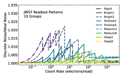
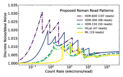
Figure 1: Ratio of the noise in the count rate using the Offenberg et al. (2001) approach used for JWST (left) and the suggested modification by Casertano (2022) for Roman (right) to the noise from the $\chi^{2}$ approach using the full covariance matrix. All current readout patterns of JWST are shown assuming 10 groups. In both cases I assume a read noise of 10 electrons/read. A fit using the full covariance matrix offers an improvement of up to $\approx$2% in signal-to-noise for JWST and between 0.5% and 3% for Roman, corresponding to increases in collecting area of up to 4% and between 2% and 6%, respectively.

The most straightforward metric of the benefit of the full covariance matrix treatment presented in this paper is the signal-to-noise ratio of the inferred count rates. Figure 1 shows the noise for the approach of Fixsen et al. (2000) and Offenberg et al. (2001) as adapted by Casertano (2022) as a fraction of the noise of a $\chi^{2}$ fit to the correct covariance matrix. The latter approach provides the smallest uncertainty of all unbiased estimates; the ratios are strictly larger than one. All currently available readout patterns for NIRCam on JWST are shown with 10 groups; the proposed Roman readout patterns are detailed in Casertano (2022). In all cases the covariance matrix itself is assumed to be known. In reality the covariance matrix must be estimated; this introduces biases that I derive in Section 5 and Appendix B. I assume a fiducial read noise of 10 electrons in a single read.

The noise values shown in Figure 1 show improvements from the discrete weighting case ranging from $\ll$1% for long JWST ramps with many reads per ramp (Deep8, with ten resultants each of eight reads) to 3% for long Roman exposures from using a fit with the full covariance matrix. Typical improvements range from 0.5% to 2%, corresponding to an increase in equivalent collecting area of 1% to 4%. These represent meaningful improvements to the missions if the full $\chi^{2}$ fit can be implemented robustly and efficiently. If the construction of the resultants themselves can be modified to accommodate weighted averages of reads, Appendix A shows that further improvements are possible especially with low numbers of resultants as would be the case if downlink bandwidth is severely restricted.

In addition to the improvement on the precision of slope fitting, the full approach presented in this paper enables a better sensitivity to jumps in the count rate from, e.g., cosmic rays. The improvement depends on the count rate and readout pattern; it is derived and discussed in Section 6.

3 Deriving the Covariance Matrix

The first task in fitting a ramp is to derive a covariance matrix for the groups of reads or, in this case, for the differences between sequential groups of reads. Throughout this paper I will refer to the average of a group of reads as a resultant. I will assume that I have many resultants $\{N_{1},\ldots,N_{n+1}\}$: the first resultant is the unweighted average of $N_{1}$ reads, etc. Appendix A shows how to treat the case of a weighted average of reads and demonstrates the potential improvement in performance. I assume $n+1$ resultants so that there are $n$ differences between adjacent resultants; this will make the notation more convenient later. The normalized difference between two successive resultants $i+1$ and $i$ is then

$$d_{i}=\frac{1}{\langle t_{i+1}\rangle-\langle t_{i}\rangle}\left(\frac{1}{N_{i+1}}\sum{\bf y}_{i+1}-\frac{1}{N_{i}}\sum{\bf y}_{i}\right)$$ (3)

where ${\bf y}_{i}$ refers to all of the reads in group $i$ and $\langle t_{i}\rangle$ is the average time of all reads that together comprise resultant $i$. The quantity $d_{i}$ has units of counts per unit time. I will assume henceforth that the counts are in units of electrons. In this section I will first derive the variance and covariance of resultants, and then transform these into the variance and covariance of resultant differences. The derivation of the covariance matrix that I present is similar to those in Kubik et al. (2015) and in Casertano (2022).

The variance of a read due to read noise is $\sigma^{2}$, where $\sigma^{2}$ is the single read variance (one-half the correlated double sampling variance). The variance of a resultant due to read noise is then

$${\rm Var}_{i}=\frac{\sigma^{2}}{N_{i}}$$ (4)

where $N_{i}$ is the number of reads in resultant $i$. The covariance between different resultants due to read noise is zero since they do not share any reads.

The covariance between two reads due to photon noise is the expected number of photons that are shared between the two reads, i.e.,

$${\rm Covar}(y_{i},y_{j})=a\cdot{\rm min}(t_{i},t_{j})$$ (5)

for a count rate $a$. For two different resultants, assuming $i<j$ and that all reads in resultant $i$ precede the first read in resultant $j$, the covariance is given by

$${\rm Covar}(r_{i},r_{j}) =\frac{a}{N_{i}N_{j}}\sum_{k=1}^{N_{i}}\sum_{l=1}^{N_{j}}{\rm min}(t_{i,k},t_{j,l})$$

$$=\frac{a}{N_{i}N_{j}}\sum_{k=1}^{N_{i}}\sum_{l=1}^{N_{j}}t_{i,k}$$

$$=\frac{a}{N_{i}}\sum_{k=1}^{N_{i}}t_{i,k}$$

$$=a\langle t_{i}\rangle.$$ (6)

The variance of a single resultant is given by

$${\rm Var}(r_{i}) =\frac{a}{N_{i}^{2}}\sum_{k=1}^{N_{i}}\sum_{l=1}^{N_{i}}{\rm min}(t_{i,k},t_{i,l}).$$ (7)

The time of the first read will appear $2N_{i}-1$ times in this double sum, $N_{i}$ times for each sum minus one from double counting. The time of the second read will appear $2N_{i}-3$ times, and so on. The variance can then be written

$${\rm Var}(r_{i}) =\frac{a}{N_{i}^{2}}\sum_{k=1}^{N_{i}}(2N_{i}-2k+1)t_{k}.$$ (8)

Following Casertano (2022) I define a variance-weighted time $\tau_{i}$ for each resultant $i$

$$\tau_{i}=\frac{1}{N_{i}^{2}}\sum_{k=1}^{N_{i}}(2N_{i}-2k+1)t_{k}$$ (9)

so that

$${\rm Var}(r_{i}) =a\tau_{i}.$$ (10)

If there are a large number of evenly spaced reads in each resultant,

$$t_{k}=t_{0}+k\frac{\Delta t}{N}$$ (11)

with the total duration of the resultant being

$$\Delta t=t_{N}-t_{1},$$ (12)

we have

$$\tau_{i} \approx\langle t_{i}\rangle-2\sum_{k=1}^{N_{i}}kt_{k}$$ (13)

and

$$\lim_{N\rightarrow\infty}\tau_{i} =\langle t_{i}\rangle-\frac{\Delta t}{6}.$$ (14)

Using Equations (6) and (8), we can now write the variance of the resultant difference $r_{i+1}-r_{i}$ and the covariance of resultant differences $r_{i+1}-r_{i}$ and $r_{j+1}-r_{j}$, including both read noise and photon noise. For the variance, we have

$${\rm Var}(r_{i+1}-r_{i}) ={\rm Var}(r_{i})+{\rm Var}(r_{i+1})-2\cdot{\rm Covar}(r_{i},r_{i+1})$$

$$=\sigma^{2}\left(\frac{1}{N_{i}}+\frac{1}{N_{i+1}}\right)+a\left(\tau_{i}+\tau_{i+1}-2\langle t_{i}\rangle\right).$$ (15)

If the resultants each last for a time $\Delta t$, consist of many reads, and occur immediately after one another, the variance becomes

$${\rm Var}(r_{i+1}-r_{i}) \approx\sigma^{2}\left(\frac{1}{N_{i}}+\frac{1}{N_{i+1}}\right)+a\left(\frac{2\Delta t}{3}\right).$$ (16)

This is slightly less than the variance from two reads evenly spaced by $\Delta t$, which would have a factor of unity in place of $\frac{2}{3}$.

For the covariance, with $j=i+1$, we have

$${\rm Covar}(r_{j+1}-r_{j},r_{i+1}-r_{i}) ={\rm Cov}(r_{i+2},r_{i+1})-{\rm Var}(r_{i+1})-{\rm Cov}(r_{i+2},r_{i})+{\rm Cov}(r_{i+1},r_{i})$$

$$=a\langle t_{i+1}\rangle-\frac{\sigma^{2}}{N_{i+1}}-a\tau_{i+1}-a\langle t_{i}\rangle+a\langle t_{i}\rangle$$

$$=-\frac{\sigma^{2}}{N_{i+1}}+a\left(\langle t_{i+1}\rangle-\tau_{i+1}\right).$$ (17)

If the resultants consist of uninterrupted sequences of many reads with no gaps between resultants, and each lasts for $\Delta t$, this covariance becomes

$${\rm Covar}(r_{j+1}-r_{j},r_{i+1}-r_{i}) \approx-\frac{\sigma^{2}}{N_{i+1}}+a\left(\frac{\Delta t}{6}\right).$$ (18)

The second term would be absent from Equation (18) for single read resultants. If $j>i+1$, we have

$${\rm Covar}(r_{j+1}-r_{j},r_{i+1}-r_{i}) ={\rm Cov}(r_{j+1},r_{i+1})-{\rm Cov}(r_{j+1},r_{i})+{\rm Cov}(r_{j},r_{i+1})-{\rm Cov}(r_{j},r_{i})$$

$$=a\langle t_{i+1}\rangle-a\langle t_{i}\rangle+a\langle t_{i+1}\rangle-a\langle t_{i}\rangle$$

$$=0.$$ (19)

In other words, only adjacent resultant differences have nonzero covariance. For notational convenience I will define

$$\delta_{i}t=\langle t_{i+1}\rangle-\langle t_{i}\rangle$$ (20)

so that $\delta_{i}t$ is the characteristic difference between the read times that form the resultant difference $d_{i}$. The scaled resultant differences are then

$$d_{i}=\frac{r_{i+1}-r_{i}}{\delta_{i}t}.$$ (21)

The covariance matrix of all of the scaled resultant differences $d_{i}$ may be written as a matrix ${\bf C}_{r}$ to be multiplied by the read noise variance $\sigma^{2}$ and a second matrix ${\bf C}_{\gamma}$ to be multiplied by the photon count rate $a$:

$${\bf C}=a{\bf C}_{\gamma}+\sigma^{2}{\bf C}_{r}.$$ (22)

The read noise matrix has components

$$\left({\bf C}_{r}\right)_{ij}=\frac{1}{\left(\delta_{i}t\right)\left(\delta_{j}t\right)}\times\begin{cases}1/N_{i}+1/N_{i+1}&i=j\\ -1/N_{j}&{j=i+1}\\ -1/N_{i}&{i=j+1}\\ 0&{|i-j|>1}\end{cases}$$ (23)

and the photon noise matrix has components

$$\left({\bf C}_{\gamma}\right)_{ij}=\frac{1}{\left(\delta_{i}t\right)\left(\delta_{j}t\right)}\times\begin{cases}\tau_{i}+\tau_{i+1}-2\langle t_{i}\rangle&i=j\\ \langle t_{j}\rangle-\tau_{j}&{j=i+1}\\ \langle t_{i}\rangle-\tau_{i}&{i=j+1}\\ 0&{|i-j|>1}\end{cases}$$ (24)

In Equation (22), ${\bf C}_{\gamma}$ and ${\bf C}_{r}$ depend only on the properties of the readout scheme: they do not need to be computed separately for every pixel. Both are tridiagonal, so the total covariance matrix ${\bf C}$ will also be tridiagonal. This fact was also pointed out by Kubik et al. (2015).

The arguments and derivations above provide the elements of the tridiagonal covariance matrix of the resultant differences ${\bf d}=\{d_{i}\}$ as

$${\bf C}=\begin{bmatrix}\alpha_{1}&\beta_{1}&0&0&\ldots\\ \beta_{1}&\alpha_{2}&\beta_{2}&0&\ldots\\ 0&\ddots&\ddots&\ddots\\ 0&\ldots&\beta_{n-2}&\alpha_{n-1}&\beta_{n-1}\\ 0&\ldots&0&\beta_{n-1}&\alpha_{n}\\ \end{bmatrix}.$$ (25)

Each element $\alpha$ and $\beta$ is the sum of a term scaled by a given pixel’s photon rate $a$ and another term scaled by the read noise variance $\sigma^{2}$:

$$\alpha_{i} =\sigma^{2}\left(\frac{1}{\left(\delta_{i}t\right)^{2}}\right)\left(\frac{1}{N_{i}}+\frac{1}{N_{i+1}}\right)+a\left(\frac{1}{\left(\delta_{i}t\right)^{2}}\right)\left(\tau_{i}+\tau_{i+1}-2\langle t_{i}\rangle\right)$$ (26)

$$\beta_{i} =\sigma^{2}\left(\frac{1}{\left(\delta_{i}t\right)\left(\delta_{i+1}t\right)}\right)\left(\frac{-1}{N_{i+1}}\right)+a\left(\frac{1}{\left(\delta_{i}t\right)\left(\delta_{i+1}t\right)}\right)\left(\langle t_{i+1}\rangle-\tau_{i+1}\right)$$ (27)

The read noise $\sigma$ may typically be measured for each pixel, but the true count rate $a$ will be unknown. For the following section I will assume that the count rate is given and will derive the slope of the best-fit ramp, its uncertainty, and its goodness-of-fit $\chi^{2}$. I will then turn to the problem of estimating the covariance matrix itself.

3.1 Including the Reset Value

The preceding discussion derived the covariance matrix for the differences of adjacent resultants. For some applications the reset value is also useful. This could be for applying a nonlinearity correction, for monitoring the detector stability, or even for using the first read to measure the count rate. The precision of measuring the count rate using the first resultant alone is limited by $kTC$ noise in the reset value.

If we wish to include the reset value, then we will also make use of the first resultant $r_{1}$. We define $d_{0}$ as

$$d_{0}\equiv\frac{r_{1}}{\langle t_{1}\rangle}$$ (28)

so that, in the absence of noise,

$$d_{0}=a+\frac{b}{\langle t_{1}\rangle}$$ (29)

where $b$ is the reset value (the counts in a pixel at $t=0$). If we wish to measure $b$, we can prepend $d_{0}$ to the vector $\left\{d_{1},\ldots,d_{n}\right\}$. We also need to prepend values to both $\alpha$ and $\beta$ for the covariance matrix. The value of $\alpha_{0}$ will be

$$\alpha_{0}=\frac{1}{\langle t_{1}\rangle^{2}}{\rm Var}\left(r_{1}\right)=\sigma^{2}\left(\frac{1}{N\langle t_{1}\rangle^{2}}\right)+a\left(\frac{\tau_{1}}{\langle t_{1}\rangle^{2}}\right)$$ (30)

while the value of $\beta_{0}$ will be

$$\beta_{0} =\frac{1}{\langle t_{1}\rangle\left(\delta_{1}t\right)}{\rm Covar}\left(r_{2},r_{1}\right)-\frac{1}{\langle t_{1}\rangle\left(\delta_{1}t\right)}{\rm Var}\left(r_{1}\right)$$

$$=\sigma^{2}\left(\frac{-1}{N\langle t_{1}\rangle\left(\delta_{1}t\right)}\right)+a\left(\frac{\langle t_{1}\rangle-\tau_{1}}{\langle t_{1}\rangle\left(\delta_{1}t\right)}\right).$$ (31)

Equations (26) and (27) may also be used directly if we take $\delta_{0}t=\langle t_{1}\rangle$ and $1/N_{0}=0$. The covariance matrix remains tridiagonal.

4 Fitting a Ramp

With the covariance matrix defined by Equation (25) via Equations (26) and (27), we want to fit the scaled resultant differences. I will defer the calculation including the reset value, which uses the additional elements of the covariance matrix given in Section 3.1, for Section 4.1.

All scaled resultant differences $d_{i}$ for $i=1,\ldots n$ should have the same value in the absence of noise assuming the astrophysical count rate to be constant and the detector to be linear and well-behaved. The likelihood of a model consisting of a single count rate $a$ is then

$$-2\ln{\cal L}=\chi^{2}=\left({\bf d}-a\cdot{\bf 1}\right)^{T}{\bf C}^{-1}\left({\bf d}-a\cdot{\bf 1}\right)$$ (32)

where ${\bf 1}$ refers to a vector of all ones. I can find the maximum likelihood count rate by differentiating this and setting it equal to zero:

$$\frac{d\chi^{2}}{da}=0=2\cdot{\bf 1}^{T}{\bf C}^{-1}\left({\bf d}-a\cdot{\bf 1}\right)$$ (33)

or

$$a=\left({\bf 1}^{T}{\bf C}^{-1}{\bf d}\right)\left({\bf 1}^{T}{\bf C^{-1}}{\bf 1}\right)^{-1}.$$ (34)

The formula for $\chi^{2}$ itself may be expanded out as

$$\chi^{2}=\left({\bf d}^{T}{\bf C}^{-1}{\bf d}\right)+2a\left({\bf 1}^{T}{\bf C}^{-1}{\bf d}\right)+a^{2}\left({\bf 1}^{T}{\bf C}^{-1}{\bf 1}\right).$$ (35)

These equations all include a matrix inverse and matrix multiplications. A general matrix inverse has a computational cost of $n^{3}$ where $n$ is the dimensionality of the matrix, while matrix multiplication with a vector has a cost of $n^{2}$. These costs could be unacceptable if there are many reads or many resultants for millions of pixels. In the following I will show that the best-fit $a$ and $\chi^{2}$ may be computed using closed formulas for a cost that is linear in the number of resultant differences $n$.

I will begin by computing the inverse of the covariance matrix, using the formula for a tridiagonal matrix. I will first define some helper variables using recursion relations (Usmani, 1994):

$$\theta_{0} =1$$ (36)

$$\theta_{1} =\alpha_{1}$$ (37)

$$\theta_{i} =\alpha_{i}\theta_{i-1}-\beta_{i-1}^{2}\theta_{i-2}$$ (38)

and

$$\phi_{n+1} =1$$ (39)

$$\phi_{n} =\alpha_{n}$$ (40)

$$\phi_{i} =\alpha_{i}\phi_{i+1}-\beta_{i}^{2}\phi_{i+2}.$$ (41)

The inverse of the covariance matrix is then given by

$$\left({\bf C^{-1}}\right)_{ij}=\begin{cases}(-1)^{i+j}\beta_{i}\cdots\beta_{j-1}\theta_{i-1}\phi_{j+1}/\theta_{n}&i<j\\ \theta_{i-1}\phi_{i+1}/\theta_{n}&i=j\\ (-1)^{i+j}\beta_{j}\cdots\beta_{i-1}\theta_{j-1}\phi_{i+1}/\theta_{n}&i>j\end{cases}.$$ (42)

I will further define

$$B_{i} =\prod_{j=1}^{i-1}\beta_{j}~{}~{}{\rm with}~{}~{}B_{1}=1$$ (43)

$$\Phi_{i} =\sum_{j=i+1}^{n}(-1)^{j}\frac{B_{j}}{B_{i}}\phi_{j+1}~{}~{}{\rm with}~{}~{}\Phi_{n}=0$$ (44)

$$\Theta_{i} =\sum_{j=0}^{i-1}(-1)^{j+1}\theta_{j}\frac{B_{i}}{B_{j+1}}$$ (45)

$$(\Theta{\rm D})_{i} =\sum_{j=1}^{i}(-1)^{j}d_{j}\theta_{j-1}\frac{B_{i}}{B_{j}}~{}~{}{\rm with}~{}~{}(\Theta{\rm D})_{0}=0$$ (46)

Each of these is computable with a cost linear in the number of resultant differences. However, they are problematic if any of the $\beta$ terms are zero. We can avoid this possibility by using the following equivalent recursion relations:

$$\Phi_{i} =\beta_{i}\Phi_{i+1}+(-1)^{i+1}\beta_{i}\phi_{i+2}$$ (47)

$$\Theta_{i} =\beta_{i-1}\Theta_{i-1}+(-1)^{i}\theta_{i-1}$$ (48)

$$\left(\Theta D\right)_{i} =\beta_{i-1}\left(\Theta D\right)_{i-1}+(-1)^{i}d_{i}\theta_{i-1}$$ (49)

with the initial conditions

$$\Phi_{n} =0$$ (50)

$$\Theta_{1} =-\theta_{0}$$ (51)

$$\left(\Theta D\right)_{0} =0$$ (52)

$$\left(\Theta D\right)_{1} =-d_{1}\theta_{0}$$ (53)

With these definitions, I will compute the terms I need to solve. First, the best-fit slope is given by

$$a=\left(\sum_{i=1}^{n}d_{i}\sum_{j=1}^{n}\left({\bf C^{-1}}\right)_{ij}\right)\left(\sum_{i=1}^{n}\sum_{j=1}^{n}\left({\bf C^{-1}}\right)_{ij}\right)^{-1}.$$ (54)

The first term in Equation (54) may be written as

$$\sum_{i=1}^{n}d_{i}\sum_{j=1}^{n}\left({\bf C^{-1}}\right)_{ij} =\sum_{i=1}^{n}d_{i}\left(\sum_{j=1}^{i}\left(-1\right)^{i+j}\frac{B_{i}\theta_{j-1}\phi_{i+1}}{B_{j}\theta_{n}}+\sum_{j=i+1}^{n}\left(-1\right)^{i+j}\frac{B_{j}\theta_{i-1}\phi_{j+1}}{B_{i}\theta_{n}}\right)$$

$$=\sum_{i=1}^{n}d_{i}\left(\left(-1\right)^{i}\frac{\phi_{i+1}}{\theta_{n}}\Theta_{i}+\left(-1\right)^{i}\frac{\theta_{i-1}}{\theta_{n}}\Phi_{i}\right)$$

$$=\sum_{i=1}^{n}d_{i}\frac{\left(-1\right)^{i}}{\theta_{n}}\left(\phi_{i+1}\Theta_{i}+\theta_{i-1}\Phi_{i}\right).$$ (55)

The second term will look just like the first term but without the $d$ factor, i.e.,

$$\sum_{i=1}^{n}\sum_{j=1}^{n}\left({\bf C^{-1}}\right)_{ij} =\sum_{i=1}^{n}\frac{\left(-1\right)^{i}}{\theta_{n}}\left(\phi_{i+1}\Theta_{i}+\theta_{i-1}\Phi_{i}\right).$$ (56)

The only term that remains to compute for $\chi^{2}$ is

$$\sum_{i=1}^{n}\sum_{j=1}^{n}d_{i}d_{j}\left({\bf C^{-1}}\right)_{ij}.$$ (57)

For this term, I will use the symmetry of the covariance matrix to write

$$\sum_{i=1}^{n}\sum_{j=1}^{n}d_{i}d_{j}\left({\bf C^{-1}}\right)_{ij} =2\sum_{i=1}^{n}\sum_{j=1}^{i-1}d_{i}d_{j}\left({\bf C^{-1}}\right)_{ij}+\sum_{i=1}^{n}d_{i}^{2}\left({\bf C^{-1}}\right)_{ii}$$

$$=2\sum_{i=1}^{n}d_{i}\sum_{j=1}^{i-1}d_{j}\left(-1\right)^{i+j}\frac{B_{i}\theta_{j-1}\phi_{i+1}}{B_{j}\theta_{n}}+\sum_{i=1}^{n}d_{i}^{2}\frac{\theta_{i-1}\phi_{i+1}}{\theta_{n}}$$

$$=2\sum_{i=1}^{n}d_{i}\sum_{j=1}^{i-1}d_{j}\left(-1\right)^{i+j}\frac{\beta_{i-1}B_{i-1}\theta_{j-1}\phi_{i+1}}{B_{j}\theta_{n}}+\sum_{i=1}^{n}d_{i}^{2}\frac{\theta_{i-1}\phi_{i+1}}{\theta_{n}}$$

$$=2\sum_{i=1}^{n}d_{i}\frac{(-1)^{i}}{\theta_{n}}\phi_{i+1}\beta_{i-1}(\Theta{\rm D})_{i-1}+\sum_{i=1}^{n}d_{i}^{2}\frac{\theta_{i-1}\phi_{i+1}}{\theta_{n}}$$ (58)

taking $\beta_{0}=1$ for the $i=1$ term of the first sum. Again, this is computable at a cost linear in the number of resultant differences.

So, to sum up, I will define

$${\cal A} =2\sum_{i=1}^{n}d_{i}\frac{(-1)^{i}}{\theta_{n}}\phi_{i+1}(\Theta{\rm D})_{i-1}+\sum_{i=1}^{n}d_{i}^{2}\frac{\theta_{i-1}\phi_{i+1}}{\theta_{n}}$$ (59)

$${\cal B} =\sum_{i=1}^{n}d_{i}\frac{\left(-1\right)^{i}}{\theta_{n}}\left(\phi_{i+1}\Theta_{i}+\theta_{i-1}\Phi_{i}\right)$$ (60)

$${\cal C} =\sum_{i=1}^{n}\frac{\left(-1\right)^{i}}{\theta_{n}}\left(\phi_{i+1}\Theta_{i}+\theta_{i-1}\Phi_{i}\right).$$ (61)

The best-fit count rate is then

$$a={\cal B}/{\cal C},$$ (62)

its standard error is

$$\sigma^{2}_{a}=1/{\cal C},$$ (63)

and the best-fit $\chi^{2}$ value is

$$\chi^{2}_{\rm best} ={\cal A}-2a{\cal B}+a^{2}{\cal C}$$

$$={\cal A}-\frac{{\cal B}^{2}}{\cal C}.$$ (64)

This section showed that I can compute the general up-the-ramp count rate with the full covariance matrix at a cost that is linear in the number of resultant differences. For a very small additional cost (evaluating the ${\cal A}$ term), I can also compute $\chi^{2}$ and see whether a constant count rate is a good fit to the data. There is no need to precompute coefficients or interpolate within different signal-to-noise regimes. The full covariance matrix will be calculated once per frame as a term that is proportional to the photon rate at a given pixel and a second term that is proportional to the read noise variance at each pixel.

4.1 Fitting the Reset Value

If we want to fit for the reset value, we use the tridiagonal covariance matrix with the additional $\alpha_{0}$ and $\beta_{0}$ defined by Equations (30) and (31), and the additional scaled resultant defined by Equation (28). The equation for $\chi^{2}$ becomes

$$\chi^{2}=\left({\bf d}-a\cdot{\bf 1}-\frac{b}{\langle t_{1}\rangle}\cdot{\bf i}\right)^{T}{\bf C}^{-1}\left({\bf d}-a\cdot{\bf 1}-\frac{b}{\langle t_{1}\rangle}\cdot{\bf i}\right)$$ (65)

where ${\bf i}$ is a vector that is one in the first entry and zero elsewhere. This may be expanded to obtain

$$\chi^{2}={\bf d}^{T}{\bf C}^{-1}{\bf d}+a^{2}\left({\bf 1}^{T}{\bf C}^{-1}{\bf 1}\right)+\frac{b^{2}}{\langle t_{1}\rangle^{2}}\left({\bf i}^{T}{\bf C}^{-1}{\bf i}\right)-2a\left({\bf 1}^{T}{\bf C}^{-1}{\bf d}\right)-2\frac{b}{\langle t_{1}\rangle}\left({\bf i}^{T}{\bf C}^{-1}{\bf d}\right)+2a\frac{b}{\langle t_{1}\rangle}\left({\bf i}^{T}{\bf C}^{-1}{\bf 1}\right).$$ (66)

Some of these terms were already computed in the first part of Section 4, allowing me to write

$$\chi^{2}={\cal A}+a^{2}{\cal C}+\frac{b^{2}}{\langle t_{1}\rangle^{2}}\left({\bf i}^{T}{\bf C}^{-1}{\bf i}\right)-2a{\cal B}-2\frac{b}{\langle t_{1}\rangle}\left({\bf i}^{T}{\bf C}^{-1}{\bf d}\right)+2a\frac{b}{\langle t_{1}\rangle}\left({\bf i}^{T}{\bf C}^{-1}{\bf 1}\right).$$ (67)

The term ${\bf i}^{T}{\bf C}^{-1}{\bf i}$ is given in Equation (42) as

$${\bf i}^{T}{\bf C}^{-1}{\bf i}=C^{-1}_{11}=\frac{\theta_{0}\phi_{2}}{\theta_{n}}$$ (68)

while ${\bf i}^{T}{\bf C}^{-1}{\bf 1}$ may be written using just the first term in the sum of Equation (61):

$${\bf i}^{T}{\bf C}^{-1}{\bf 1}\equiv{\cal C}^{\prime}_{1}=\frac{-1}{\theta_{n}}\left(\phi_{2}\Theta_{1}+\theta_{0}\Phi_{1}\right).$$ (69)

In all of these formulas the $\beta$ and $\alpha$ values prepended to the arrays in Equations (26) and (27) are indexed by 1. In other words, where $\beta_{1}$ appears in these equations, it now refers to the value in Equation (31), and where $d_{1}$ appears, it refers to the value in Equation (28).

To write the remaining term in Equation (67) more conveniently, I will define one additional quantity

$$\left(\Phi D\right)_{j}=\sum_{i=j+1}^{n}(-1)^{i}d_{i}\phi_{i+1}\frac{B_{i}}{B_{j}}~{}~{}{\rm with}~{}~{}\left(\Phi D\right)_{n-1}=0.$$ (70)

As for the terms in Equations (44)–(46), this is equivalently defined by the recursion relation

$$\left(\Phi D\right)_{n-1} =0$$ (71)

$$\left(\Phi D\right)_{j} =\beta_{j}\left(\Phi D\right)_{j+1}+\left(-1\right)^{j+1}\beta_{j}d_{j+1}\phi_{j+2}$$ (72)

which avoids the possibility of division by zero. With this definition, I can write

$${\bf d}^{T}{\bf C}^{-1}{\bf i}\equiv{\cal B}^{\prime}_{1}=\frac{-1}{\theta_{n}}\left(\phi_{2}(\Theta D)_{1}+\theta_{0}(\Phi D)_{1}\right)$$ (73)

and finally

$$\chi^{2}={\cal A}+a^{2}{\cal C}+\frac{b^{2}}{\langle t_{1}\rangle^{2}}C^{-1}_{11}-2\frac{b}{\langle t_{1}\rangle}{\cal B}^{\prime}_{1}-2a{\cal B}+2a\frac{b}{\langle t_{1}\rangle}{\cal C}^{\prime}_{1}.$$ (74)

In some cases, there may be a prior placed on the reset value $b$. If the reset value is stable up to $kTC$ noise and only the first resultant is usable, then the use of a prior on $b$ is the only way to obtain a constraint on the count rate $a$. Assuming a Gaussian prior with a mean of $z$ and an uncertainty $\sigma_{z}$, the expression for $\chi^{2}$ becomes

$$\chi^{2}={\cal A}+a^{2}{\cal C}+\frac{b^{2}}{\langle t_{1}\rangle^{2}}C^{-1}_{11}-2\frac{b}{\langle t_{1}\rangle}{\cal B}^{\prime}_{1}-2a{\cal B}+2a\frac{b}{\langle t_{1}\rangle}{\cal C}^{\prime}_{1}+\frac{\left(b-z\right)^{2}}{\sigma_{z}^{2}}.$$ (75)

Setting $z=0$ and $\sigma_{z}=\infty$ recovers the case of a uniform prior on the reset value.

The first step to computing the best $\chi^{2}$ is to differentiate $\chi^{2}$ and set the result equal to zero:

$$\frac{\partial\chi^{2}}{\partial a} =0=2a{\cal C}-2{\cal B}+2\frac{b}{\langle t_{1}\rangle}{\cal C}^{\prime}_{1}$$ (76)

$$\frac{\partial\chi^{2}}{\partial b} =0=2\frac{b}{\langle t_{1}\rangle^{2}}C^{-1}_{11}-2{\cal B}^{\prime}_{1}+2\frac{a}{\langle t_{1}\rangle}{\cal C}^{\prime}_{1}+2\left(\frac{b-z}{\sigma_{z}^{2}}\right).$$ (77)

This yields

$$b =\left({\cal B}^{\prime}_{1}-\frac{{\cal C}^{\prime}_{1}{\cal B}}{{\cal C}\langle t_{1}\rangle^{2}}+\frac{z}{\sigma^{2}_{z}}\right)\left(\frac{C_{11}^{-1}}{\langle t_{1}\rangle^{2}}-\frac{{\cal C}_{1}^{\prime 2}}{{\cal C}\langle t_{1}\rangle^{2}}+\frac{1}{\sigma_{z}^{2}}\right)^{-1}$$ (78)

$$a =\frac{\cal B}{\cal C}-b\left(\frac{{\cal C}^{\prime}_{1}}{{\cal C}\langle t_{1}\rangle}\right).$$ (79)

The covariance matrix for $a$ and $b$ is then

$${\bf C}^{-1}(a,b) =\begin{bmatrix}\frac{1}{2}\frac{\partial^{2}\chi^{2}}{\partial a^{2}}&\frac{1}{2}\frac{\partial^{2}\chi^{2}}{\partial a\partial b}\\ \frac{1}{2}\frac{\partial^{2}\chi^{2}}{\partial a\partial b}&\frac{1}{2}\frac{\partial^{2}\chi^{2}}{\partial b^{2}}\end{bmatrix}$$

$$=\begin{bmatrix}{\cal C}&{\cal C}^{\prime}_{1}/\langle t_{1}\rangle\\ {\cal C}^{\prime}_{1}/\langle t_{1}\rangle&C^{-1}_{11}/\langle t_{1}\rangle^{2}+1/\sigma_{z}^{2}\end{bmatrix}.$$ (80)

This may be inverted by hand to get the standard errors on $a$ and $b$ and their covariance.

4.2 Omitting One or More Resultant Differences

Sometimes a resultant difference is corrupted, e.g., by a cosmic ray: there can be a jump in counts between two resultants. There can also be a jump within a resultant, in which case two resultant differences must be discarded (both of the differences that contain the resultant with a jump). Saturation of a pixel or of its neighbor can also corrupt all resultant differences after the onset of saturation.

Sometimes the resultant differences that should not be used are known in advance of fitting a ramp. Saturation is a good example, as this phenomenon can be independently flagged. Jump detection algorithms can identify cosmic ray hits and specify resultant differences to be discarded. Section 6 will discuss a new approach to jump detection, but that will involve an iterative approach requiring the capability of discarding resultant differences flagged in previous iterations.

One way of discarding a resultant difference is to write down a new covariance matrix that is block diagonal but omits the corrupted difference. This covariance matrix would be specified by a different set of $\alpha$ and $\beta$ values, and with a different dimension (one less for each discarded resultant difference), making it more difficult to implement the equations presented here as array operations. It also makes it considerably more difficult to keep track of indices specifying which resultant difference corresponds to which $\alpha$ and $\beta$.

I adopt a different approach. Assuming that we wish to discard resultant difference $j$, i.e. $d_{j}$, I first decouple $d_{j}$ from the other differences by setting $\beta_{j-1}=\beta_{j}=0$. This renders the covariance matrix block diagonal. The inverse of the covariance matrix now has elements in row/column $j$

$$C^{-1}_{jk}=C^{-1}_{kj}=\frac{1}{\alpha_{j}}\delta_{jk}$$ (81)

where $\delta_{jk}$ is the Kronecker delta. We need to set these to zero or to ensure that terms containing them are zero. The elements within the sum for ${\cal C}$ in Equation (61) are the column-summed elements of ${\bf C}^{-1}$; so we can set the $j$ term to zero (equivalently, we can set $\Theta_{j}=\Phi_{j}=0$). For ${\cal B}$ and ${\cal A}$, the only resultant difference that multiplies the $j$ row or column of ${\bf C}^{-1}$ is $d_{j}$, so we can set $d_{j}=0$.

In sum, if we wish to ignore resultant difference $j$, we set

$$\beta_{j-1}=\beta_{j}=\Theta_{j}=\Phi_{j}=d_{j}=0.$$ (82)

We can do this for any number of resultant differences and continue to apply the equations derived above. This statement holds true whether or not we are fitting for the reset value.

5 Biases and Estimating the Covariance Matrix

Sections 3 and 4 assumed that the covariance matrix is known. In general the read noise of each pixel may be accurately known, but that pixel’s true count rate will not be known. The covariance matrix must first be approximated using the resultants themselves. This could introduce biases. In this section I will compute those biases to first order and show that fitting for the count rate using two iterations effectively avoids them. While it is not directly relevant to this paper, the case of discretely varying weighting schemes to estimate the count rate, as presented by Fixsen et al. (2000) and refined by Casertano (2022) among others, is also biased. The intuition for this bias and its calculation can provide grounding and context for the case at hand; they are presented in Appendix B.

For the present approach I will start with Equation (54), the formula for a ramp, and define

$$w_{i}=\left(\sum_{j}\left({\bf C^{-1}}\right)_{ij}\right)\left(\sum_{j}\sum_{k}\left({\bf C^{-1}}\right)_{jk}\right)^{-1}.$$ (83)

where the covariance matrix only applies to the resultant differences. I then have

$$a=\sum_{i}w_{i}d_{i}={\bf w}\cdot{\bf d}$$ (84)

$$\sum_{i}w_{i}=1.$$ (85)

The $w_{i}$ are themselves functions of the count rate $a$ assumed in the construction of the covariance matrix (for the photon noise portion). For the rest of this discussion I will assume that the (unknown) actual count rate is $\tilde{a}$ while the covariance matrix is derived using a slightly different $a^{\prime}$. I will assume that the read noise associated with each pixel is accurately known.

I will first treat the case where the $a^{\prime}$ used in the construction of the covariance matrix is not directly derived from any of the resultant differences $d_{i}$. In this case, I can use the fact that

$$\langle d_{i}\rangle=\tilde{a}$$ (86)

for all reads $i$ because the observed count rate is an unbiased estimator of the true count rate and because read noise has zero mean. Equations (84), (85), and (86) then imply that the $\chi^{2}$-minimizing fit gives an unbiased estimator of the flux:

$$\langle a\rangle =\bigg{\langle}\sum_{i}w_{i}d_{i}\bigg{\rangle}$$

$$=\sum_{i}w_{i}\langle d_{i}\rangle$$

$$=\sum_{i}w_{i}\tilde{a}$$

$$=\tilde{a}.$$ (87)

This does not hold if the $w_{i}$ depend on the values of $d_{i}$, i.e., if the $d_{i}$ values are used in determining the count rate for the purposes of deriving the covariance matrix. In that case, I will assume that the covariance matrix is calculated assuming a photon rate of

$$a^{\prime}=\sum_{i}c_{i}d_{i}={\bf c}\cdot{\bf d}$$ (88)

with

$$\sum_{i}c_{i}=1.$$ (89)

This is fairly general: if all $c_{i}$ are equal then this is the case of using the average count rate (scaled differences between adjacent groups of reads) to compute the covariance matrix; it is equivalent to using the difference between the first and last groups of reads. Iteratively updating $w_{i}$ and estimating $a$ would correspond to another set of $c_{i}$ (different at each iteration). Using weights for each resultant derived from the read-noise limited fit would correspond to a different set of $c_{i}$.

The dependence of the weights $w_{i}$ on the adopted value of $a$ is complicated so I will use a Taylor expansion of $w_{i}$ to first order about the true count rate $\tilde{a}$. I have

$$\langle a\rangle =\Bigg{\langle}\sum_{i}\left(w_{i}(\tilde{a})+\frac{dw_{i}}{da}\left(\left(\sum_{j}c_{j}d_{j}\right)-\tilde{a}\right)\right)d_{i}\Bigg{\rangle}$$

$$=\tilde{a}+\Bigg{\langle}\sum_{i}d_{i}\frac{dw_{i}}{da}\left(\sum_{j}c_{j}\left(d_{j}-\tilde{a}\right)\right)\Bigg{\rangle}$$ (90)

where I used $\sum c_{j}=1$, $\langle d_{i}\rangle=\tilde{a}$, and $\sum w_{i}=1$. I will further expand this by subtracting and adding $\tilde{a}$ to $d_{i}$:

$$\langle a\rangle =\tilde{a}+\Bigg{\langle}\sum_{i}\left(d_{i}-\tilde{a}\right)\frac{dw_{i}}{da}\left(\sum_{j}c_{j}\left(d_{j}-\tilde{a}\right)\right)\Bigg{\rangle}+\tilde{a}\Bigg{\langle}\sum_{i}\frac{dw_{i}}{da}\left(\sum_{j}c_{j}\left(d_{j}-\tilde{a}\right)\right)\Bigg{\rangle}$$

$$=\tilde{a}+\Bigg{\langle}\sum_{i}\sum_{j}c_{j}\frac{dw_{i}}{da}\left(d_{j}-\tilde{a}\right)\left(d_{i}-\tilde{a}\right)\Bigg{\rangle}+\tilde{a}\Bigg{\langle}\sum_{i}\sum_{j}c_{j}\frac{dw_{i}}{da}\left(d_{j}-\tilde{a}\right)\Bigg{\rangle}$$

$$=\tilde{a}+\sum_{i}\sum_{j}c_{j}\frac{dw_{i}}{da}\big{\langle}\left(d_{j}-\tilde{a}\right)\left(d_{i}-\tilde{a}\right)\big{\rangle}+\tilde{a}\sum_{i}\sum_{j}c_{j}\frac{dw_{i}}{da}\big{\langle}\left(d_{j}-\tilde{a}\right)\big{\rangle}.$$ (91)

The last term is zero because the individual scaled resultant differences are unbiased estimators of the true count rate. The first term has the covariance matrix of the resultant differences:

$$\langle a\rangle =\tilde{a}+\sum_{i}\sum_{j}c_{j}\frac{dw_{i}}{da}{\rm Cov}(d_{i},d_{j}).$$ (92)

So, if we adopt a covariance matrix built using a weighted sum of the resultant differences to estimate the photon rate, then Equation (92) gives a first-order estimate of the bias introduced to the recovered count rate. It is possible to either correct for this bias or to choose a set of weights $c_{j}$ for the initial estimate of the count rate in order to have zero bias to first order. If we want to avoid the bias, then we wish to choose a vector of initial guess coefficients ${\bf c}$ so that ${\bf c}$ is orthogonal to

$${\bf v}\equiv{\bf C}\frac{d{\bf w}}{da}.$$ (93)

In fact, the set of optimal coefficients ${\bf w}$ to combine the resultant differences is a bias-free choice for ${\bf c}$. To prove this I will use the fact that the weights ${\bf w}$ given in Equation (83) provide the minimum-variance unbiased estimate of the true count rate if the true covariance matrix is ${\bf C}$ (Aitken, 1935). The variance of the sum of resultant differences weighted by ${\bf w}$ is the variance of the recovered count rate $a$, and is given by

$$\sigma^{2}_{a}={\bf w}^{T}{\bf C}{\bf w}.$$ (94)

A weight vector ${\bf w}^{\prime}$ derived with a different assumed count rate (i.e. a different approximation to the true covariance matrix) will still produce an unbiased estimate of the count rate due to Equation (87). In other words, ${\bf w}(a)$ gives an unbiased estimate of the true count rate for any assumed count rate $a$ used to approximate the covariance matrix and, from this, compute ${\bf w}$ using Equation (83). The Gauss-Markov theorem then states that $\sigma^{2}_{a}$ is minimized if the weight vector ${\bf w}$ is derived using the true count rate $a_{\rm true}$. So, differentiating $\sigma^{2}_{a}$ with respect to the count rate used to derive ${\bf w}$ will equal zero at $a_{\rm true}$:

$$0 =\frac{d}{da}\left({\bf w}^{T}{\bf C}{\bf w}\right)$$

$$=\left(\frac{d{\bf w}}{da}\right)^{T}{\bf C}{\bf w}+{\bf w}^{T}{\bf C}\frac{d{\bf w}}{da}$$

$$=2{\bf w}^{T}{\bf C}\frac{d{\bf w}}{da}$$ (95)

where the last line used the symmetry of the covariance matrix ${\bf C}={\bf C}^{T}$. So, if the optimal weight vector ${\bf w}$ can be approximately calculated, then the covariance matrix computed from $a={\bf w}\cdot{\bf d}$ allows for a nearly unbiased estimate of the true count rate. If the covariance matrix is approximated using $a={\bf c}\cdot{\bf d}$ for some other ${\bf c}$, then the resulting best-fit count rate will be biased by an amount

$${\rm bias}\approx{\bf c}^{T}{\bf C}\frac{d{\bf w}}{da}.$$ (96)

The bias of Equation (96) results from a series expansion of ${\bf w}$ about the true count rate $a$. Negative values of $a$ are incompatible with the Poisson distribution; the covariance matrix should not have a negative coefficient times the photon noise covariance matrix. In practice this means that Equation (96) overestimates the bias when the count rate is close to zero assuming that the covariance matrix is approximated using the maximum of $a={\bf c}\cdot{\bf d}$ and zero.

5.1 Empirical Demonstrations of the Bias

I have tested the first-order approximation for the bias on synthetic data with 30 reads each treated individually. The off-diagonal elements of the covariance matrix in this case consist only of read noise. I further adopt a read noise of $\sigma=20$ electrons. The bias will depend upon the actual count rate (which partially determines the covariance matrix ${\bf C}$) and on the weight vector ${\bf c}$ used to estimate the count rate for use in approximating the covariance matrix.

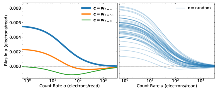
Figure 2: Biases computed using Equation (96) for a sequence of 30 individual reads with a read noise of 20 electrons using various initial weight vectors ${\bf c}$. Left panel: the ${\bf c}$ vectors are set to the optimal weights for three different true count rates. Right panel: biases for 50 random vectors ${\bf c}$ with all elements drawn from $U(0,1)$ and the vector finally normalized to a unit sum. The bias can be significant at low count rates depending on the weights on the resultant differences used to estimate the covariance matrix. The bias is zero when the vector ${\bf c}$ is the optimal weight vector for the actual count rate.

Figure 2 plots the bias computed using Equation (96) as a function of count rate for several different initial weight vectors ${\bf c}$. The left panel shows the bias resulting from the optimal weight vector for zero count rate, a moderate count rate of 20 electrons/read, and an arbitrarily high count rate for which all elements of ${\bf c}$ are the same. The right panel of Figure 2 shows the bias resulting from 50 random realizations of the initial weight vector ${\bf c}$. In all cases, I use uniform random numbers between zero and one for all elements and then normalize the vector so that the elements sum to one. The biases in both cases can be non-negligible at low count rates.

At very low count rates (indistinguishable from zero), the bias drops by half because the count rate used for computing the covariance matrix cannot be negative. This is not captured in Equation (96) so the horizontal axis of Figure 2 only shows count rates for which the signal-to-noise ratio on the best-fit count rate is at least 1.5. In practice Equation (96) overestimates the bias when the signal-to-noise ratio on the best-fit count rate is low.

Next, I test the bias calculated using Equation (96) with Monte Carlo. For this I use a count rate of 2 electrons/read. For my initial estimate of the count rate, I simply average all of the resultant differences together with uniform weights. This is equivalent to taking the total number of counts and dividing by the total integration time. It is the optimal estimate at high photon rates, and we therefore expect it to produce unbiased count rates in this regime. At low photon rates, however, this weighting is not optimal and it can produce biases. Equation (92) gives a bias of $\approx$0.25% on the best-fit slope, or 0.00521 on a true slope of 2. This is verified by Monte Carlo simulations. Generating and fitting $10^{7}$ ramps produced a mean best-fit slope of 2.00515 with an uncertainty on the mean of 0.00016. At a true count rate of zero, Equation (92) gives a bias of 0.00561. The actual bias in $10^{7}$ ramps generated with no true counts was 0.00280 with a standard error on the mean of 0.00013. The bias is half of the prediction because $d{\bf w}/da=0$ only exists as a right-handed derivative. At low but nonzero count rates, the actual bias is a factor between $\frac{1}{2}$ and 1 times that given by Equation (92).

I can remove the bias to first order by computing Equation (93), projecting this vector off of my initial weight vector, renormalizing the weight vector, and repeating the Monte Carlo test. This does not give the optimal weight vector but it does give one that will produce an estimate of the covariance matrix that results in unbiased fitted count rates. Using this approach with another $10^{7}$ synthetic ramps, the mean best-fit slope becomes 2.00015 with an uncertainty on the mean of 0.00016, i.e., the bias is more than 10 times lower and is no longer detectable without running a much larger set of synthetic ramps.

I can also avoid almost all of the bias by performing the fit to the ramp twice. I use the first fit to infer the weights ${\bf w}$, and after using these weights to estimate the photon rate, I recompute the covariance matrix. I then use this new covariance matrix to perform a second fit to the ramp in order to compute the final count rate. This approach applied to $10^{7}$ synthetic ramps with a true slope of 2 produced a mean best-fit slope of 2.00008 with an uncertainty on the mean of 0.00016. In agreement with Equation (95), using the optimal weights to estimate the covariance matrix results in a count rate free from bias.

To obtain the best estimate of the true photon rate and avoid biases in the process, I therefore suggest the following procedure:

1. Use uniform weights or a median on all scaled resultant differences $d_{i}$ to estimate a count rate;

2. Use this count rate to estimate the covariance matrix and fit for the count rate;

3. Use this updated count rate to re-estimate the covariance matrix; and

4. Perform the optimal fit with this re-estimated covariance matrix.

The total computational cost of this approach is approximately double the cost of fitting the ramp once.

6 Cosmic Ray Detection via Hypothesis Testing

Equation (64) gives the $\chi^{2}$ value of the best-fitting model. The availability of $\chi^{2}$ enables hypothesis testing and provides a straightforward goodness of fit measurement. In this section, I will restrict the discussion to the case where the reset value is not being fit, i.e., where $d_{1}$ refers to the scaled difference between the first and second resultants. In the case of a uniform prior on the reset value the results would be identical. The fit has one free parameter (the count rate), so the number of degrees of freedom is the number of resultant differences minus one. The survival function of this $\chi^{2}$ distribution can provide a natural flag for bad fits.

The availability of $\chi^{2}$ also enables hypothesis testing through likelihood ratios. In this section I develop one application of this hypothesis testing: searching for cosmic rays that manifest as instantaneous jumps in the counts at a given pixel. The approach is equivalent to $y$-intercept approach explored by Anderson & Gordon (2011) but the algorithms provided here are more efficient.

6.1 Cosmic Ray Detection Between Resultants

A jump in the count rate is a sudden increase in the number of counts between reads. When fitting a line to the accumulated counts, this requires fitting an offset between two ramps of identical slopes. In the framework outlined here, it means omitting the resultant difference that is corrupted by the jump. If a jump happened in the middle of a group of reads (within a resultant), two differences—both of the ones that use the contaminated group—will need to be discarded. This can either be done by fitting one additional free parameter per resultant difference to be discarded, or by omitting these resultant differences (which alters the covariance matrix). I will take the former approach here.

In this section I will work out the best-fit slope, its uncertainty, and the best-fit $\chi^{2}$ when omitting one resultant difference by giving it an additional free parameter. I will assume that the resultant difference to be omitted is $j$ and use ${\bf j}$ to denote a vector that is zero except for element $j$, where it is one. The new expression for $\chi^{2}$ is

$$\chi^{2} =\left({\bf d}-a_{j}{\bf 1}-b_{j}{\bf j}\right)^{T}{\bf C}^{-1}\left({\bf d}-a_{j}{\bf 1}-b_{j}{\bf j}\right)$$

$$={\bf d}^{T}{\bf C}^{-1}{\bf d}+a_{j}^{2}\cdot{\bf 1}^{T}{\bf C}^{-1}{\bf 1}+b_{j}^{2}\cdot{\bf j}^{T}{\bf C}^{-1}{\bf j}-2b_{j}\cdot{\bf d}^{T}{\bf C}^{-1}{\bf j}-2a_{j}\cdot{\bf d}^{T}{\bf C}^{-1}{\bf 1}+2a_{j}b_{j}\cdot{\bf j}^{T}{\bf C}^{-1}{\bf 1}.$$ (97)

This closely matches Equation (66), and I take the same approach to minimize $\chi^{2}$ and compute the covariance matrix. I generalize three terms defined in Section 4.1 to any read $j$:

$${\bf j}^{T}{\bf C}^{-1}{\bf j}={C}^{-1}_{jj}=\frac{\theta_{j-1}\phi_{j+1}}{\theta_{n}},$$ (98)

$${\bf j}^{T}{\bf C}^{-1}{\bf 1}\equiv{\cal C}^{\prime}_{j}=\frac{\left(-1\right)^{j}}{\theta_{n}}\left(\phi_{j+1}\Theta_{j}+\theta_{j-1}\Phi_{j}\right),$$ (99)

and

$${\bf d}^{T}{\bf C}^{-1}{\bf j}\equiv{\cal B}^{\prime}_{j}=\frac{\left(-1\right)^{j}}{\theta_{n}}\left(\phi_{j+1}(\Theta D)_{j}+\theta_{j-1}(\Phi D)_{j}\right).$$ (100)

This allows us to write the expression for $\chi^{2}$ as

$$\chi^{2}={\cal A}+a_{j}^{2}{\cal C}+b_{j}^{2}C^{-1}_{jj}-2b_{j}{\cal B}^{\prime}_{j}-2a_{j}{\cal B}+2a_{j}b_{j}{\cal C}^{\prime}_{j}.$$ (101)

All sums only need to be computed once for the ramp, not once per $j$. As a result, computing $\chi^{2}$ at all $j$, i.e., at all possible locations of a jump in the counts, is linear in the number of resultants.

I will now derive the best-fit $\chi^{2}$, the corresponding slope, and its uncertainty. By computing the best-fit $\chi^{2}$ at all possible jump locations we can perform rigorous hypothesis testing using all available information. Sometimes there can be jumps within the reads that make up a resultant. In that case, two resultant differences must be discarded since both have the corrupted resultant. This case is somewhat messier but its computational complexity remains linear in the number of resultants. It is treated in Appendix C.

The first step to computing the best $\chi^{2}$ is to differentiate $\chi^{2}$ and set the result equal to zero:

$$\frac{\partial\chi^{2}}{\partial a_{j}} =0=2a_{j}{\cal C}-2{\cal B}+2b_{j}{\cal C}^{\prime}_{j}$$ (102)

$$\frac{\partial\chi^{2}}{\partial b_{j}} =0=2b_{j}C^{-1}_{jj}-2{\cal B}^{\prime}_{j}+2a_{j}{\cal C}^{\prime}_{j}$$ (103)

This yields

$$a_{j} =\frac{C^{-1}_{jj}{\cal B}-{\cal B}^{\prime}_{j}{\cal C}^{\prime}_{j}}{{\cal C}C^{-1}_{jj}-\left({\cal C}^{\prime}_{j}\right)^{2}}$$ (104)

$$b_{j} =\frac{{\cal B}^{\prime}_{j}-a_{j}{\cal C}^{\prime}_{j}}{C^{-1}_{jj}}.$$ (105)

These expressions can be efficiently and simultaneously computed at all possible $j$ values. They may then be substituted into Equation (101) to derive the best $\chi^{2}$ possible by omitting each possible resultant difference.

The final step is to derive the standard uncertainty on the best-fit count rate. To do this I will first derive the covariance matrix of $a_{j}$ and $b_{j}$ as

$${\bf C}^{-1}(a_{j},b_{j}) =\begin{bmatrix}\frac{1}{2}\frac{\partial^{2}\chi^{2}}{\partial a_{j}^{2}}&\frac{1}{2}\frac{\partial^{2}\chi^{2}}{\partial a_{j}\partial b_{j}}\\ \frac{1}{2}\frac{\partial^{2}\chi^{2}}{\partial a_{j}\partial b_{j}}&\frac{1}{2}\frac{\partial^{2}\chi^{2}}{\partial b_{j}^{2}}\end{bmatrix}$$

$$=\begin{bmatrix}{\cal C}&{\cal C}^{\prime}_{j}\\ {\cal C}^{\prime}_{j}&C^{-1}_{jj}\end{bmatrix}.$$ (106)

This finally gives the standard uncertainty on $a_{j}$ as

$$\sigma^{2}(a_{j})=\frac{C^{-1}_{jj}}{{\cal C}C^{-1}_{jj}-({\cal C}^{\prime}_{j})^{2}}.$$ (107)

The value of $b_{j}$ may also be useful, e.g., if fitting for the morphology of a cosmic ray hit to correct pixels where the hit induced only a small perturbation to the ramp. In this case, the uncertainty in $b_{j}$ may also be of value; it is given by

$$\sigma^{2}(b_{j})=\frac{\cal C}{{\cal C}C^{-1}_{jj}-({\cal C}^{\prime}_{j})^{2}}.$$ (108)

6.2 A Practical Approach for Multiple Jumps

The preceding subsection showed how to compute $\chi^{2}$ when leaving out a single resultant difference. This is suitable for a jump that occurred between resultants, which is always the case when each resultant is a single read. If a resultant consists of more than one read, a cosmic ray could arrive in the middle of the resultant. In this case two resultant differences—both of the ones that contain the contaminated resultant—must be discarded. Appendix C contains the full treatment of discarding two adjacent resultant differences from the analysis. It is conceptually the same as excluding one resultant difference but the equations are slightly more complicated.

A real ramp could have more than one jump, and its resultants could contain a mixture of single reads and multiple reads. In this case we need an iterative approach, and we need to treat resultants differently. Here I propose a cosmic ray flagging and removal algorithm that satisfies both criteria.

The first step in my proposed approach is to treat single read resultants and multiple read resultants differently. It will search for cosmic ray hits between single read resultants (potentially discarding only one difference), but will require both resultant differences containing a multiple read resultant to be discarded. This could be modified for a readout scheme with more than read per resultant, but with long gaps between resultants such that jumps remain likely to occur between resultants. In all cases, a fit excluding single resultant differences or pairs of resultant differences will improve the $\chi^{2}$ value of the fit because it removes one or two constraints. If this $\chi^{2}$ improvement exceeds a user-defined threshold for any resultant in a ramp, then a single difference will be discarded. The discarded measurement will be the resultant difference or pair of differences whose $\chi^{2}$ improvement most exceeds the user-specified threshold. This difference or pair of differences can then be masked for another iteration, with the process continuing until no additional resultant differences are flagged.

A step-by-step approach of the algorithm above follows:

1. Using the method in Section 6 and Appendix C, identify the resultant difference or pair of differences most likely to hold a jump, i.e., the one whose omission most improves $\chi^{2}$. For a difference of single read resultants only one resultant difference will be omitted, while for a resultant containing two or more reads two adjacent differences will be omitted. For this step, estimate the covariance matrix using the median of the resultant differences for the count rate. If the estimated photon count rate is negative set it to zero.

2. Determine whether the improvement in $\chi^{2}$ from omitting this resultant difference, indexed by $j$, exceeds a user-specified significance threshold. When comparing the possibility of discarding a single resultant difference vs. two differences, the one that offers the largest $\chi^{2}$ improvement over the relevant user-specified threshold will be chosen.

3. If the resultant difference $j$ or pair of differences $j,j+1$ that offers the greatest $\chi^{2}$ improvement exceeds the user-specified threshold, discard it from the analysis using the approach of Section 4.2.

4. Return to Step 1 and iterate until no resultant difference or differences exceeds the adopted significance threshold, or until the ramp contains two or fewer resultant differences. If there are only two resultant differences remaining there is no way to tell which one is correct and which contains a jump. In this case, the entire ramp is corrupted.

5. After discarding all flagged resultant differences, adopt the resulting count rate, its uncertainty, and $\chi^{2}$ value for that pixel.

For Step 3, we must also explicitly set $C^{-1}_{jj}=0$ in addition to the methodology of Section 4.2. This will result in expressions containing $0/0$ for $a$, $b$, and/or $c$ if any of the relevant resultant differences are ignored in a later iteration. In that case, the given resultant difference was already excluded in a calculation with one fewer resultant difference omitted. We can therefore fill in these values with the corresponding count rates, $\chi^{2}$ values, and uncertainties from our prior calculation that did not doubly omit a resultant difference.

After applying this sequence of steps, the user can re-estimate the covariance matrix one final time with the count rates from Step (5) to obtain the final count rates and uncertainties. This removes biases in the count rates to first order as discussed in Section 5.

The approach outlined above requires no modification of the core equations of Section 4. It does require running the algorithm several times for those pixels with more than one jump, with a total computational cost a factor of a few times the cost of fitting a single ramp once. It is also well-suited to taking ramps that have already had most jumps identified and checking for any additional, lower signal-to-noise ratio jumps.

The equations in this section and in Appendix C give the best-fit $\chi^{2}$, the best-fit count rate and its standard uncertainty leaving out any individual resultant difference or pair of adjacent differences. The results for all possible omitted resultants may be computed for a computational cost linear in the number of reads, i.e., for a similar cost to computing the best-fit count rate in the first place. This renders a full, likelihood-based cosmic ray detection algoirthm computationally straightforward. Section 8 discusses the computational cost in more detail.

7 Illustration of the Jump Fitting Algorithm and Demonstration of Effectiveness

The algorithm outlined in the preceding section can identify jumps by the $\chi^{2}$ improvement yielded by excluding one or two resultant differences at a time. Whether one or two differences are excluded depends on whether either resultant consisted of two or more reads. In this section I show examples of the performance this technique enables. I will compare to an algorithm restricted to looking at the differences between adjacent resultants and flagging them if they exceed a threshold. For my example here I use a threshold of 4.5 times the root variance of a resultant difference. If a resultant difference exceeds the median resultant difference over the ramp by at least 4.5 times the root variance of a single difference, then we discard that difference. My choice of the median rather than the mean for the baseline resultant difference is to limit the bias in the reference count rate from the presence of a jump. The mean is more sensitive to outliers introduced by the jumps themselves; this comes with a corresponding loss of sensitivity. Repeating the analysis of the following section with means rather than medians degrades sensitivity to jumps, typically by a few percent.

I will show two cases separately. First, I will consider a long ramp composed of individual reads. In this case one resultant difference may be left out at a time. Second, I will consider a shorter ramp in which each resultant consists of several reads.

7.1 Single-Read Resultants

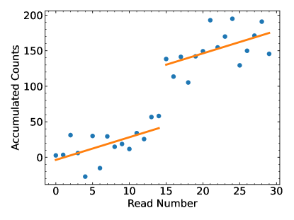
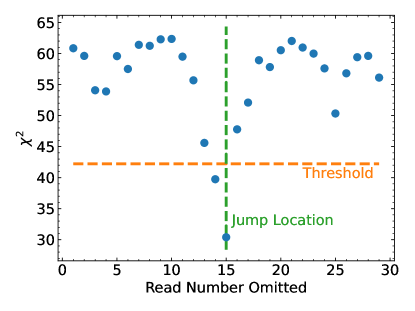
Figure 3: Demonstration of the likelihood-based jump detection algorithm. Left panel: the ramp showing the accumulated counts with the best-fit slope also shown. The slope was fitted to the read differences using the proper covariance matrix; the offsets are approximate. Right panel: $\chi^{2}$ of the fit to the read differences as a function of the read pair omitted. The orange line marked “Threshold” denotes an improvement to $\chi^{2}$ corresponding to 4.5$\sigma$ significance. The green dashed line shows where I added a jump; the jump is 3 times the uncertainty in the single read difference (CDS read noise plus photon noise added in quadrature). Omitting the read with the jump offers the maximal improvement in $\chi^{2}$, and results in a formally good $\chi^{2}$ of 30.4 for 30 reads: 29 read differences with one not used and one fitted parameter, for 27 degrees of freedom.

I will begin by illustrating the likelihood-based approach on a 30-read ramp in which I have added a discrete jump at the 15th read (indexed from zero). Figure 3 shows the accumulated counts in the left panel, and the $\chi^{2}$ value of the best-fit line as a function of the read difference that is left out. There is a large improvement to $\chi^{2}$ when leaving out the 15th read difference, exactly the one that in which I added a jump. I have marked an improvement in $\chi^{2}$ of 20.25, which corresponds to 4.5$\sigma$. If any point exceeds this threshold then the read difference that offers the maximal improvement to $\chi^{2}$ when left out of the fit is labeled as a jump.

To test the sensitivity of this approach to jumps we need to define a threshold in $\chi^{2}$ improvement over the single ramp at which we will label a jump significant. If we want the equivalent of 4.5 $\sigma$, we can use a $\chi^{2}$ threshold of 20.25; this enables a natural comparison with an algorithm that looks for individual read differences that are at least 4.5$\sigma$ discrepant with the average. This significance threshold is shown in Figure 3.

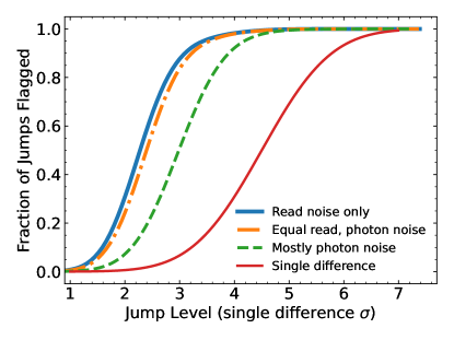
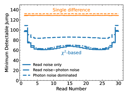
Figure 4: Comparison of jump detection efficiency on 30 read ramps. The three sets of thicker lines use the likelihood approach with a threshold of a $\chi^{2}$ improvement of 20.25 when omitting a read; this is equivalent to 4.5$\sigma$. Equal read and photon noise refers to the contributions over the ramp rather than in an individual difference (which is then dominated by read noise). The “mostly photon noise” case has a photon rate 10 times that of the equal contributions case; read noise is still important in individual differences between reads. The thinner red line shows the performance of a single difference between adjacent reads with a 4.5$\sigma$ threshold.

Figure 4 shows the results of a full sensitivity analysis. With 30 reads and in the photon noise limit, the likelihood-based jump detection is approximately twice as sensitive (on average) as the single difference approach. This change in sensitivity depends on where in the ramp the jump occurs. If the jump occurs in the middle of the reads the likelihood approach offers a larger sensitivity gain. This is also the location at which the jump would induce the maximum increase in the best-fit count rate. With more than 30 reads the advantage of the likelihood-based approach over the single difference approach grows: it becomes a factor of $\approx$2.4 at 50 reads, and $\approx$3.3 at 100 reads (assuming read noise is still significant). The single difference approach only reaches the sensitivity of the likelihood-based approach when photon noise dominates the uncertainty in individual read differences rather than just in the entire ramp. This only occurs for very high count rates. The right panel of Figure 4 shows the jump that is detected 50% of the time as a function of its position within a 30-read ramp. The single difference approach is equally sensitive everywhere, while the $\chi^{2}$ approach is most sensitive near the middle of the ramp where the jump would induce the maximal bias on the inferred count rate.

7.2 Intra-resultant vs. inter-resultant sensitivity

I now turn to the case of a shorter ramp in which each resultant is composed of multiple reads. In this case the likelihood-based algorithm will omit two resultant differences at a time, both of the ones that include the resultant that is being investigated for a jump. For this example I will consider a ramp of ten resultants with a jump in one of the resultants other than the first and last one. I will compute the sensitivity of the algorithm to a jump as a function of the time of the cosmic ray hit, for resultants each composed of six reads, and for resultants each composed of many reads.

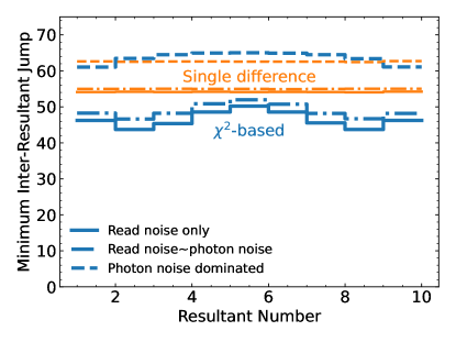
Figure 5: Median sensitivity to a jump that occurs between resultants using either the $\chi^{2}$ approach presented here (blue steps) or a single resultant difference (orange steps). The line styles show results assuming only read noise (solid lines), equal photon and read noise when combined over the ramp (dot-dashed lines), and photon noise ten times read noise, again, over the entire ramp (dashed lines). In the latter case photon noise dominates slightly over read noise in each individual resultant difference. A resultant consists of six reads each with a read noise of 20 electrons. Because the $\chi^{2}$ approach discards two resultant differences for multi-read resultants it can be slightly less sensitive than the single difference approach for the same false positive rate if a jump occurs between resultants. This is evident in the middle reads in the photon noise dominated case.

Figure 5 shows the sensitivity of both the $\chi^{2}$-based approach presented here and a single resultant difference to a jump between resultants. The figure shows the jump that is detected 50% of the time assuming a read noise of 20 electrons and six reads per resultant. In the photon noise dominated case photon noise dominates over the entire ramp, and is slightly larger than read noise in an individual resultant difference. For the middle resultants the $\chi^{2}$-based approach appears to be slightly worse than the single difference approach. The thresholds of the two approaches have the same false positive rates, but the $\chi^{2}$ approach discards two resultant differences rather than one for its hypothesis test and must use a slightly higher significance threshold to compensate. It is only correct to discard one resultant difference if it is known that the jump occurred between resultants; this can be difficult to assess. For jumps that occur within a resultant the single difference threshold approach to jump detection must be followed by a decision to discard either one or both of the resultant differences on either side of the flagged difference. This step is unnecessary for the $\chi^{2}$ approach as it tests pairs of excluded differences.

A jump in the middle of a resultant is more difficult to detect than a jump between resultants. The additional counts are diluted: the resultant with the jump only contains half of the extra counts that it would have if the jump happened just before the first read of the resultant. The difference between resultants likewise consists of smaller jumps by up to a factor of 2. A single-difference search is limited by these facts, while a likelihood approach can do better because it can account for the jump across more the one resultant difference.

Here I compare a single resultant difference threshold with my $\chi^{2}$-based likelihood approach for a jump that occurs within a resultant. I again compute the jump level that will be flagged 50% of the time and choose thresholds that result in consistent false positive rates between the two approaches. To show the difference in sensitivity as a function of jump time within a resultant, I normalize sensitivities to the inter-resultant sensitivity at which both approaches are most sensitive to jumps. I exclude the first and last resultants from this analysis. A jump within the first or last resultant is both more difficult to detect and shows little difference between the $\chi^{2}$ approach and the single difference approach. Both of these are because only a single resultant difference is available.

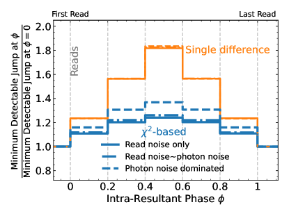
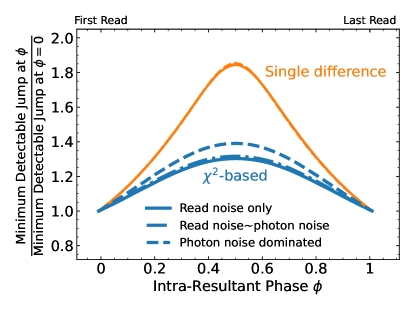
Figure 6: Left panel: minimum detectable jump at 50% efficiency as a function of its position within a 6-read resultant in a 10 resultant ramp; the jump level is normalized to its value between resultants (where efficiency is maximized). Right panel: the same plot for 10 resultants each composed of a large number of reads. A detection algorithm only using a single resultant difference loses almost half its sensitivity when a jump happens halfway through a resultant. In this case the peak resultant difference is half of its value for a cosmic ray that hits between resultants. The median sensitivity drops by slightly less than a factor of two because there is an extra chance to get a favorable realization of noise to add to the jump. The $\chi^{2}$ approach described here is substantially more sensitive especially when read noise is important.

Figure 6 shows the results for six-read resultants on the left and for many-read resultants on the right. The single-difference approach suffers from almost a factor of two loss in sensitivity for a jump that occurs in the middle of a multi-read resultant. The signal is a factor of two lower than for a jump between resultants, but with two equal differences (one on either side of the resultant with the jump), one is likely to have a noise realization that adds to the difference caused by the jump. For independent Gaussian noise of variance $\sigma^{2}/2$ in each resultant (i.e. variance $\sigma^{2}$ in each resultant difference), the larger of two adjacent resultant differences has a median of $0.64\sigma$. Assuming a threshold of $4.5\sigma$ this would give a ratio of intra-resultant to inter-resultant sensitivity of

$$\frac{2\times(4.5-0.64)}{4.5}\approx 1.71.$$ (109)

where the factor of 2 in the numerator is because only half of the jump occurs in each difference. This effect is partially countered by the fact that the reference count rate must be estimated from the reads themselves. The median of the scaled read differences is biased high relative to the true count rate because one or two of these differences contain contributions from a jump. This bias is $\approx$0.3$6\sigma$ when two of nine resultant differences are biased many sigma high by a jump; it is $\approx$0.1$5\sigma$ when only one of nine resultant differences is biased high. This increases the ratio of the intra-resultant to the inter-resultant sensitivity to slightly more than 1.8, in closer agreement with Figure 6. Biases in the count rate also produce overestimated noise values and reduce sensitivity, slightly increasing the sensitivity ratio to its value of almost 1.85 in Figure 6.

The $\chi^{2}$ approach is significantly more sensitive than a single difference threshold, especially where read noise dominates. Because the $\chi^{2}$ approach uses both differences containing the resultant with a jump, it is a factor $\approx\sqrt{2}$ more sensitive than using single-result differences when the resultants have negligible covariance.

The $\chi^{2}$ approach has an additional advantage over a single difference threshold. The $\chi^{2}$ approach omits two resultant differences at a time; it excludes both differences affected by the resultant containing a jump. In this way it identifies the specific resultant containing the jump: the one that is shared between the two omitted differences. A single difference threshold identifies a difference containing the resultant with a jump. However, it does not identify which of the two resultants contributing to this difference contains the jump. A jump near the end of the first resultant looks identical to a jump near the beginning of the second resultant. As a result, two resultants (three resultant differences) might need to be excluded, rather than one resultant (two differences) with the $\chi^{2}$ approach.

8 A Pure Python Implementation

I have implemented the algorithms described in this paper, both for ramp fitting and for jump detection, in pure Python. In this section I briefly summarize the implementation and its computational cost. All tests running the code were performed on a 2020 Macbook Air. I have further included a series of tests to verify that all calculations are correct: that the calculated covariance matrix agrees with a Monte Carlo approximation, that the best-fit slopes agree with the results of explicit matrix inversion, and that cosmic ray rejection successfully identifies and removes jumps put in by hand.

The first step in my implementation is to compute the $\alpha$ and $\beta$ components of the covariance matrix and the $\delta t$ values for a set of read times. This set of read times is a list of the time(s) corresponding to each resultant. A single read resultant may be specified by either a floating point number for the read time or a list of numbers for a multiple-read resultant. The resulting $\alpha$ and $\beta$ components for photon noise and read noise are then stored in a specifically designed Python class.

The next step is to fit a ramp. The corresponding function takes a 2D array of resultant differences (number of resultants minus one by number of pixels), the Python class holding the covariance information from the read times, and the read noise of each pixel. It is vectorized to operate on many pixels simultaneously. Optionally, this step may include a mask of the same shape as the resultant differences (differences with a mask value of zero are ignored), and it can compute count rates and $\chi^{2}$ values leaving out resultant differences and pairs of differences.

For cosmic ray detection, I have implemented the iterative jump detection algorithm described in Section 6. This function is built on the ramp fitting function described in the preceding paragraph. Finally, I have included a Python method to compute the bias in the count rate from using a weighted average of the resultant differences to estimate the count rate for the covariance matrix.

Implementing the ramp fitting and cosmic ray rejection algorithms described in this paper requires computing a number of auxiliary quantities. These quantities, defined throughout this paper, all have a linear cost in the number of resultants. They also require memory. To limit the memory footprint, I recommend using the ramp fitting and jump detection algorithms on one row of detector pixels at a time. A row-by-row loop also enables more efficient memory access compared to trying to access large parts of many different arrays that exist in distant regions of RAM. In practice I have found maximal efficiency from operating on $10^{3}$–$10^{4}$ pixels at a time. This approach leaves a negligible memory footprint.

The computational cost of this approach, while larger than simply averaging resultant differences, is modest and is linear in the number of resultants. For that reason the performance numbers I quote are in units of seconds per $10^{8}$ pixel-resultants. A ramp with twice as many resultants will take twice as long to process, as will a ramp with twice as many pixels. A ramp with $10^{8}$ pixel-resultants roughly corresponds, for example, to an H2RG ($\approx 4\times 10^{6}$ pixels) with 24 resultants.

Running my pure Python implementation on a single core of a 2020 Macbook Air takes $\approx$2.6 seconds per $10^{8}$ pixel-resultants to fit a ramp once. Fitting a ramp twice to remove bias doubles this cost to a little over five seconds per $10^{8}$ pixel-resultants. Running cosmic ray detection takes $\approx$9 seconds per $10^{8}$ pixel-resultants without, or $\approx$12 seconds per $10^{8}$ pixel-resultants with, one additional fit to remove bias. For an H4RG ramp with 10 resultants this cost corresponds to $\sim$8 seconds to fit a ramp and remove bias, or $\approx$20 seconds to perform a full cosmic ray cleaning. The time to perform a full cosmic ray cleaning scales modestly with the number of cosmic ray hits, rising to $\approx$40 seconds when cosmic rays affect 10% of the resultant differences. These times correspond to a 2.5-year-old laptop and could be considerably lower on a better computer. They would be correspondingly lower for ramps taken from a smaller H2RG detector.

8.1 Numerical Considerations

The computations needed to calculate the best-fit slope, its uncertainty, and $\chi^{2}$ are given by the equations of Section 4. For a diagonally dominant matrix (as all covariance matrices that will arise for realistic ramps are) these typically do not present numerical difficulties.

If the photon rate and/or read noise are large, then overflow is a risk. For example, assuming one read per second,

$$\theta_{n}\sim\left({\rm max}\left(a,\sigma^{2}\right)\right)^{n}.$$ (110)

If $n=100$ and $\sigma^{2}=10000$ (for a very long ramp with a very noisy pixel) then overflow could result. If necessary, overflow (and, less likely, underflow) can be avoided by factoring the geometric mean of $\alpha$ out of the covariance matrix. This will not affect the best-fit slope. However, the uncertainty on the best-fit slope and the value of $\chi^{2}$ will both need to be multiplied by this factor after they are computed. My current implementation does not take this additional step to limit the risk of floating point overflow.

9 Conclusions

Past work in the literature has either approximated the optimal solution to the problem of fitting a ramp (Fixsen et al., 2000; Kubik et al., 2016; Casertano, 2022), or has required expensive matrix operations (e.g. Robberto, 2014). Here I have shown that the optimal approach can be implemented with a computationally efficient algorithm. Closed-form solutions for the weights of the reads are available, and the computational costs are linear in the number of resultants. The optimal approach does require the covariance matrix of the resultants to be estimated first; this can introduce a bias in the best-fit count rate. I have derived a formula for the bias and shown how it can be removed to first order.

As a byproduct of deriving the optimal count rates, I have also shown that the $\chi^{2}$ values of the fits may be computed for little additional cost. This enables straightforward flags for the goodness of fit. It also enables hypothesis testing for the presence of a cosmic ray manifested as a jump in the counts at a pixel. This hypothesis testing uses the entire ramp to test every possible resultant that could host a jump, but has a computational cost linear in the number of resultants. It outperforms algorithms based on single resultant differences especially for long ramps and for jumps that occur in the middle of a resultant.

The algorithms presented here can be implemented efficiently in pure Python. They are computationally straightforward on a laptop computer even for long ramps on a large-format detector. This could enable more straightforward and sensitive ramp fitting and cosmic ray detection for existing and future instruments using detectors that are read out nondestructively.

Appendix A Nonuniform Weighting Within a Resultant

The analysis in Sections 3 and 4 assumes that the individual reads within a resultant are averaged, with each read contributing equally. This does not have to be the case, and a weighted average of the reads can offer better performance. In this section I show that, assuming an ideal detector subject to read noise and photon noise, an alternative weighting approach can always outperform resultants that are composed of equally weighted reads. The quantitative discussion of jumps in Section 6 will use the case of equally weighted resultants, though the formulas in Section 3 straightforwardly generalize to nonuniform weights; the formulas and approach of Sections 4, 5, and 6 would be identical.

Equally weighting each read within a resultant is never the optimal approach when the final goal is to fit a ramp. In this section I will show that other weighting schemes can outperform equal weighting for all count rates and for all readout schemes. I will focus on the optimal weighting in the read noise limited case. These weights are straightforward to implement, always outperform uniform weighting, and remain compatible with suppression algorithms for correlated read noise and cosmic rays. In the limit of low signal, this approach achieves the same signal-to-noise ratio on read noise limited data as saving all of the reads.

I will start by deriving the optimal coefficients for an up-the-ramp fit with $N$ reads at $N$ times $\{t_{1},\ldots,t_{N}\}$ assuming only read noise. The number of counts in a pixel, neglecting noise, should then be

$$y_{i}=at_{i}+b.$$ (A1)

I will write down $\chi^{2}$ as

$$\chi^{2}=\sum_{i}\frac{\left(y_{i}-at_{i}-b\right)^{2}}{\sigma^{2}}.$$ (A2)

I can find the best-fit slope by differentiating $\chi^{2}$ with respect to $a$ and $b$ and setting the derivatives equal to zero. The solution for $a$ may be written

$$a=\frac{1}{N\left(\overline{t^{2}}-\overline{t}^{2}\right)}\left(\sum_{i}t_{i}y_{i}-\overline{t}\sum_{i}y_{i}\right)$$ (A3)

with

$$\overline{t} \equiv\frac{1}{N}\sum_{i}t_{i}$$ (A4)

$$\overline{t^{2}} \equiv\frac{1}{N}\sum_{i}t_{i}^{2}.$$ (A5)

The coefficient that multiplies each read is then

$$c_{i}=\frac{t_{i}-\overline{t}}{N\left(\overline{t^{2}}-\overline{t}^{2}\right)}.$$ (A6)

If there is more than one read in a resultant, optimal intra-resultant weights may be defined by

$$\kappa_{i} =\frac{c_{i}}{\sum_{i\in{\rm res}}c_{i}}$$

$$=\frac{t_{i}-\overline{t}}{\sum_{i\in{\rm res}}\left(t_{i}-\overline{t}\right)}$$ (A7)

where $\overline{t}$ refers to the average read time of all of the reads in the ramp. The total weight within a resultant is constrained to be one, and if there is only one read in a resultant, it will continue to have unit weight.

Each resultant will now be a weighted average of reads. The covariances derived in Section 3 must therefore be generalized. For read noise the generalization is straightforward, with

$${\rm Var}({\bf r}_{i})=\sigma^{2}\sum_{j}\kappa_{i,j}^{2},$$ (A8)

where $j$ runs over the reads within resultant $i$, taking the place of Equation (4). For photon noise, the covariance between resultant $i$ and resultant $i+1$ is

$${\rm Cov}({\bf r}_{i},{\bf r}_{i+1})=a\left(\sum_{j}\kappa_{i,j}t_{i,j}\right)\equiv a\langle t_{i}\rangle$$ (A9)

which simplifies to Equation (6) if the $\kappa$ values are all equal (in which case the new and old definitions of $\langle t_{i}\rangle$ are equivalent). The variance of resultant $i$ due to read noise is

$${\rm Var}({\bf r}_{i})=a\sum_{j}\sum_{k}\kappa_{i,j}\kappa_{i,k}{\rm min}(t_{i,j},t_{i,k}).$$ (A10)

This expression takes the place of Equation (7), which can no longer be simplified. These equations may be propagated through the remainder of the derivations in Section 3 to derive the appropriate values for $\alpha$ and $\beta$ that define the covariance matrix.

The covariance matrix will remain tridiagonal unless a resultant has weights that sum to zero. In that case, Equation (A7) is undefined. Adopting Equation (A7) without the denominator would not solve the problem. Two of the four terms in Equation (19) (either the first two or the last two) would be zero and the sum would no longer vanish. This numerical problem may be avoided by slightly changing the weight of one of the reads while keeping $\sum\kappa_{i}=1$; a small change to the weights entails a negligible penalty in performance.

I can now measure the performance of uniform weights against the performance of nonuniform weights within each resultant. Figure 7 shows the results for the same proposed Roman readout patterns shown in Figure 1. Using the intra-resultant weights given in Equation (A7) matches the signal-to-noise ratio from using all of the reads in the low count rate limit. At all count rates, it gives superior results to uniform intra-resultant weighting. This is because in all cases the best weights increase toward the first and last reads; the optimal low count rate weights give the most gradual increase in weights toward either end. This approach is still closer to the optimal photon noise limit of only using the first and last read than is the case of uniform weights within each resultant.

The proposed intra-resultant weights given in Equation (A7) are not the only possible choices. Weights could also be optimized for intermediate count rates. In this case, slightly improved signal-to-noise ratios at higher count rates would come at the expense of slightly degraded signal-to-noise ratios at low count rates.

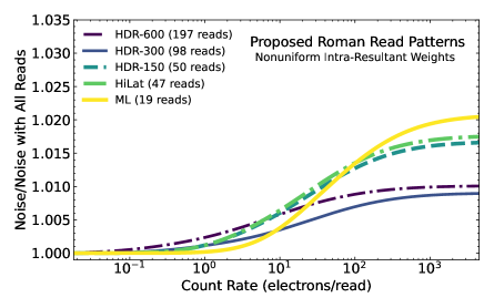
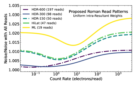
Figure 7: Left: Ratio of optimal slope fit to the optimal slope fit with all of the reads assuming uniform intra-resultant weights. The different colors show the same proposed Roman readout patterns used in Figure 1. Right: the same ratio but with intra-resultant weights optimized in the low count rate regime. The signal-to-noise ratio now reaches the value when using all of the reads for low count rates, and it is superior to the signal-to-noise for uniform intra-resultant weights at all count rates.

Nonuniform weighting within resultants can improve the final signal-to-noise ratio at all count rates, significantly so for shorter exposures at low count rates. The use of nonuniform weights will not affect the properties or removal of the correlated noise endemic to HxRG detectors, because these weights would still be the same for all pixels. Cosmic ray flagging, discussed in Section 6, will similarly be unaffected in principle. Sensitivitities to cosmic rays will change slightly, but a detailed analysis of that is beyond the scope of the current discussion. A reweighting could complicate nonlinearity corrections though, if the nonlinear behavior is accurately known, this could be propagated through the known readout and weighting pattern.

As shown in this section, nonuniform weighting within a resultant offers promise for preserving more useful information in a limited number of resultants. In the read noise limit it can preserve all useful information. If nonuniform weighting can be implemented in practice, it could improve the performance of a mission limited by downlink bandwidth.

Appendix B Biases with Approximate Weights: The Discrete Case

The ramp-fitting approach of Fixsen et al. (2000), Offenberg et al. (2001), and Casertano (2022) uses fixed weights for the different resultants, with the weights determined by the signal-to-noise ratio as estimated by the difference between the first and last resultants. The use of discrete weights does introduce biases in the recovered count rate near the signal-to-noise ratios at which the weights are discontinuous. This section provides intuition for the source of the bias and then presents a calculation of its magnitude as a function of the read noise, the true count rate, and the readout pattern.

A bias exists because the estimated count rate is a weighted sum of the resultants, but this is covariant with the difference between the first and the last resultants which is used to determine the weights. I will use $s$ to denote the difference between the last and first resultants. The signal-to-noise ratio estimate used by Casertano (2022) is

$${\rm SNR}={\rm max}\left(0,\frac{s}{\sqrt{s+\sigma^{2}}}\right)$$ (B1)

where $\sigma^{2}$ is the read noise. The estimate of the count rate is a weighted sum of the resultants,

$$a=\sum_{i}w_{i}r_{i}.$$ (B2)

Different sets of weights are used depending on the signal-to-noise ratio inferred from $s$. The inferred count rate $a$ will be covariant with $s$. As the signal-to-noise ratio increases, the first and last resultants are weighted more heavily in the sum of Equation (B2) and this covariance becomes stronger. Near a break in the weighting scheme the joint distribution of $a$ and $s$ then has a discontinuity along a line of constant $s$: the covariance above this line is larger than the covariance below this line. A joint distribution that is symmetric far from any discontinuity in the weighting scheme becomes asymmetric near a discontinuity.

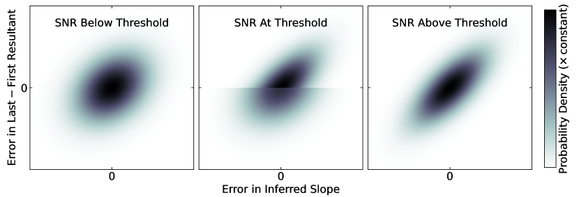
Figure 8: Illustration of the phenomenon that leads to bias when using weights that vary discontinuously to estimate the count rate. The weights used depend on the difference between the first and last resultant ($y$-axis). The error in this quantity is covariant with the error in the inferred slope. When the weights used are independent of the count rate, this covariance leads to an error ellipse and zero an expectation value of zero for the error in the inferred count rate. Near a threshold between two weighting schemes, however, two different Gaussians are combined, and the expectation of the error in the inferred slope can be nonzero.

Figure 8 illustrates the idea expressed above. Far from a discontinuity in the weights, the joint distribution of $a$ and $s$ is symmetric and its center-of-mass is at zero error in both directions. Near a discontinuity, however, this is no longer the case. The center of mass of this distribution is at zero error in $s$ (because this uncertainty remains symmetric), but it is no longer a zero error in $a$. The larger covariance at larger measured values of $s$ leads to an expectation value of the error in $a$ that is greater than zero, i.e., a positive bias. I now proceed to calculate this bias.

To calculate the bias we first need the variance of $s$, the variance of $a$, and the covariance of $s$ and $a$. The variance of $a$ is given in Casertano (2022) while the variance of $s$ is given in Section 3. Their covariance is given by

$${\rm Cov}(s,a) =\sum_{i}w_{i}\left({\rm Cov}(r_{n+1},r_{i})-{\rm Cov}(r_{1},r_{i})\right)$$

$$=w_{n+1}\left({\rm Var}\left(r_{n+1}\right)-{\rm Cov}\left(r_{n+1},r_{1}\right)\right)+w_{1}\left({\rm Covar}\left(r_{n+1},r_{1}\right)-{\rm Var}\left(r_{1}\right)\right)+\sum_{i=2}^{n}w_{i}\left({\rm Cov}(r_{n+1},r_{i})-{\rm Cov}(r_{1},r_{i})\right)$$

$$=w_{n+1}\left(a\tau_{n+1}-a\langle t_{1}\rangle+\sigma^{2}\right)+w_{1}\left(a\langle t_{1}\rangle-a\tau_{1}-\sigma^{2}\right)+\sum_{i=2}^{n}aw_{i}\left(\langle t_{i}\rangle-\langle t_{1}\rangle\right)$$ (B3)

where $r_{1}$ and $r_{n+1}$ denote the first and last resultant, respectively. The joint distribution between $s$ and $a$ is then given by the covariance matrix

$${\bf\Sigma}=\begin{bmatrix}\sigma^{2}_{s}&{\rm Covar}(s,a)\\ {\rm Covar}(s,a)&\sigma^{2}_{a}\end{bmatrix}.$$ (B4)

I will denote the elements of the inverse of this matrix as

$${\bf\Sigma}^{-1}=\begin{bmatrix}m_{11}&m_{12}\\ m_{21}&m_{22}\end{bmatrix}$$ (B5)

with $m_{12}=m_{21}$. The covariance matrix will differ above and below any threshold in $s$; I will assume that there is a discontinuity at $s=\mu$, and that the elements of $\bf\Sigma$ above and below $\mu$ are denoted by $m$ and $m^{\prime}$, respectively. In this case the expectation value of the error on $a$, $a-\tilde{a}$, is

$$\langle a-\tilde{a}\rangle= \int_{-\infty}^{\infty}a\,da\int_{-\infty}^{\mu}\frac{ds}{2\pi\sqrt{\rm det\bf\Sigma^{\prime}}}\exp\left(-\frac{1}{2}\left(m^{\prime}_{11}s^{2}+m^{\prime}_{22}a^{2}+2m^{\prime}_{12}sa\right)\right)$$

$$\qquad+\int_{-\infty}^{\infty}a\,da\int_{\mu}^{\infty}\frac{ds}{2\pi\sqrt{\rm det\bf\Sigma}}\exp\left(-\frac{1}{2}\left(m_{11}s^{2}+m_{22}a^{2}+2m_{12}sa\right)\right).$$ (B6)

I will focus only on the second term, which I will denote $\langle a-\tilde{a}\rangle_{+}$. The first term may be equivalently written with limits on $s$ from $-\mu$ to $\infty$ by replacing $s$ with $-s$. I first complete the square and integrate over $a$:

$$\langle a-\tilde{a}\rangle_{+}=\int_{\mu}^{\infty}\frac{ds}{2\pi\sqrt{\rm det\bf\Sigma}}\int_{-\infty}^{\infty}\left(a+\frac{m_{12}}{m_{22}}s-\frac{m_{12}}{m_{22}}s\right)\,da\exp\left(-\frac{m_{22}}{2}\left(a+m_{12}/m_{22}s\right)^{2}-\frac{s^{2}}{2}\left(m_{11}-\frac{m_{12}^{2}}{m_{22}}\right)\right).$$ (B7)

The odd portion of this function integrates to zero, while the even portion is an ordinary Gaussian integral. I will also use the facts that

$$\frac{m_{22}}{m_{11}m_{22}-m_{12}^{2}} =\sigma^{2}_{s}$$ (B8)

$$\frac{-m_{12}}{m_{11}m_{22}-m_{12}^{2}} ={\rm Cov}(s,a)$$ (B9)

$$\frac{1}{m_{11}m_{22}-m_{12}^{2}} ={\rm det}{\bf\Sigma}$$ (B10)

This allows me to write

$$\langle a-\tilde{a}\rangle_{+} =\int_{\mu}^{\infty}\frac{s\,ds}{2\pi\sqrt{\rm det\bf\Sigma}}\int_{-\infty}^{\infty}\left(-\frac{m_{12}}{m_{22}}\right)\,da\exp\left(-\frac{m_{22}}{2}\left(a+\frac{m_{12}}{m_{22}}s\right)^{2}-\frac{s^{2}}{2\sigma^{2}_{s}}\left(\frac{m_{11}m_{22}-m_{12}^{2}}{m_{22}}\right)\right)$$

$$=-\frac{m_{12}}{\sqrt{2\pi m_{22}^{3}{\rm det}\bf\Sigma}}\int_{\mu}^{\infty}s\,ds\exp\left(-\frac{s^{2}}{2\sigma^{2}_{s}}\right)$$

$$=\frac{m_{12}}{m_{22}}\frac{1}{\sqrt{2\pi\sigma^{2}_{s}}}\sigma^{2}_{s}\exp\left(-\frac{\mu^{2}}{2\sigma^{2}_{s}}\right)$$

$$=\frac{{\rm Covar}(s,a)}{\sqrt{2\pi\sigma^{2}_{s}}}\exp\left(-\frac{\mu^{2}}{2\sigma^{2}_{s}}\right).$$ (B11)

Finally, I use this result to compute the bias near a transition between two different weighting regimes. Denoting the covariance above the threshold as ${\rm Cov}_{+}(s,a)$ and the covariance below the threshold as ${\rm Cov}_{-}(s,a)$, and assuming the difference between $s$ and its threshold value to be $\mu$, I have

$$\langle a-\tilde{a}\rangle=\left(\frac{{\rm Covar}_{+}\left(s,a\right)-{\rm Covar}_{-}\left(s,a\right)}{\sqrt{2\pi\sigma^{2}_{s}}}\right)\exp\left(-\frac{\mu^{2}}{2\sigma^{2}_{s}}\right).$$ (B12)

This is maximised when $s$ is at a transition between weighting schemes, in which case the exponent is zero.

Two or more transitions between weighting regimes can contribute to the bias. If two transitions contribute, the bias is given by a sum of integrals of the form

$$\langle a-\tilde{a}\rangle=\int_{-\infty}^{\mu}f_{1}(s)\,ds+\int_{\mu}^{\nu}f_{2}(s)\,ds+\int_{\nu}^{\infty}f_{3}(s)\,ds$$ (B13)

where, e.g., $f_{1}$ is the integrand in the first regime (c.f. the first line of Equation (B11)), and $\mu$ and $\nu$ are the number of standard deviations the noiseless value of $s$ is away from a transition. The functions $f_{1}$, $f_{2}$, etc. are odd functions of $s$ (c.f. the second line of Equation (B11)). Using this fact, Equation (B13) can be written

$$\langle a-\tilde{a}\rangle =\int_{-\infty}^{\mu}f_{1}(s)\,ds+\int_{\mu}^{\infty}f_{2}(s)\,ds-\int_{\nu}^{\infty}f_{2}(s)\,ds+\int_{\nu}^{\infty}f_{3}(s)\,ds$$

$$=\int_{\mu}^{\infty}\left(f_{2}(s)-f_{1}(s)\right)\,ds+\int_{\nu}^{\infty}\left(f_{3}(s)-f_{2}(s)\right)\,ds.$$ (B14)

The first and second integrals each give the same result as Equation (B12) across the two respective transitions. The total bias is then the sum of Equation (B12) over both transitions. This argument can be extended to show that the total bias is the sum of Equation (B12) calculated over all transitions.

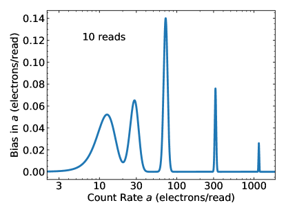
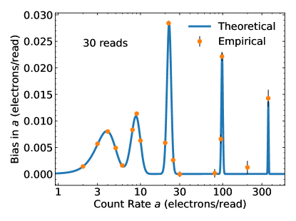
Figure 9: The bias in the discrete weighting scheme of Fixsen et al. (2000) as adapted by Casertano (2022), for 10 reads (left) and 30 reads (right) with a read noise of 20 electrons. The orange points are the averages of $5\times 10^{6}$ Monte Carlo realizations each with read and photon noise; they confirm the accuracy of the bias derived in this section. The bias is positive because a larger $s$, the difference between the first and last resultants, results in an increased weighting of these resultants in the computation of $a$, and a larger covariance between $s$ and $a$. The peaks are centered at the transitions between weighting schemes while the widths of the peaks are given by $\sigma_{s}\approx\sqrt{s+\sigma^{2}}$ scaled to the total number of reads. The width is a weakly increasing function of the count rate and appears to narrow because of the logarithmic axis.

Figure 9 shows the bias for ramps of 10 and of 30 reads. For this calculation I have used the weighting schemes and signal-to-noise ratio thresholds given in Casertano (2022), and have adopted a read noise of 20 electrons. The bias is mostly due to the read noise component of the covariance. For ten reads, the bias can be $\approx$0.5% at count rates near the boundaries between different weighting schemes. The orange points in Figure 9 show empirical calculations of the bias using Monte Carlo; they verify the accuracy of the theoretical curve derived in this section.

As for the continuous case discussed in Section 5, the bias can be mostly removed from the discrete weighting schemes. The difference in covariance between $a$ and $s$ is a linear combination of the weights (c.f. Equation (B3)). The quantity $s$, the difference between the first and last reads, results in a biased estimate of $a$. A general estimator for $a$ would have a covariance with $a$ that is likewise given by a linear combination of the weights $\{w_{i}\}$. The dimensionality of this set of estimators is one less than the number of resultants. Given a number of transitions $N$ less than the number of resultants, it is possible to choose an estimator for $a$ for which the covariance difference with $a$ is zero across all $N$ transitions. Such an estimator would produce a nearly unbiased way of choosing which weights to apply.

Appendix C Fitting a Ramp With Two Omitted Resultant Differences

In this section I derive the formulas for the best-fit count rate, its uncertainty, and the $\chi^{2}$ of the fit when omitting two adjacent resultant differences. The expression for $\chi^{2}$ becomes

$$\chi^{2}=\left({\bf d}-a{\bf 1}-b{\bf j}-c{\bf k}\right){\bf C}^{-1}\left({\bf d}-a{\bf 1}-b{\bf j}-c{\bf k}\right)$$ (C1)

where ${\bf j}$ is a vector that is zero except for the $j$ element which is one, and ${\bf k}$ is a vector that is zero except for the $k$ element which is one, with $k=j+1$. This corresponds to freely fitting for the actual resultant differences $j$ and $j+1$ so that they have no influence on the count rate. I can multiply this out to obtain

$$\chi^{2} ={\bf d}^{T}{\bf C}^{-1}{\bf d}+a^{2}\cdot{\bf 1}^{T}{\bf C}^{-1}{\bf 1}+b^{2}\cdot{\bf j}^{T}{\bf C}^{-1}{\bf j}+c^{2}\cdot{\bf k}^{T}{\bf C}^{-1}{\bf k}-2a\cdot{\bf d}^{T}{\bf C}^{-1}{\bf 1}-2b\cdot{\bf d}^{T}{\bf C}^{-1}{\bf j}$$

$$\qquad\qquad-2c\cdot{\bf d}^{T}{\bf C}^{-1}{\bf k}+2ab\cdot{\bf 1}^{T}{\bf C}^{-1}{\bf j}+2ac\cdot{\bf 1}^{T}{\bf C}^{-1}{\bf k}+2bc\cdot{\bf j}^{T}{\bf C}^{-1}{\bf k}$$ (C2)

$$={\cal A}+a^{2}{\cal C}+b^{2}C^{-1}_{jj}+c^{2}C^{-1}_{kk}-2a{\cal B}-2b{\cal B}^{\prime}_{j}-2c{\cal B}^{\prime}_{k}+2ab{\cal C}^{\prime}_{j}+2ac{\cal C}^{\prime}_{k}+2bcC^{-1}_{jk}.$$ (C3)

All of these have already been computed apart from

$$C^{-1}_{jk}=C^{-1}_{j,j+1}=-\frac{\beta_{j}\theta_{j-1}\phi_{j+2}}{\theta_{n}}.$$ (C4)

Differentiating $\chi^{2}$ to find the best-fit $a$, $b$, and $c$, I have

$$\frac{1}{2}\frac{\partial\chi^{2}}{\partial a} =0=a{\cal C}+b{\cal C}^{\prime}_{j}+c{\cal C}^{\prime}_{k}-{\cal B}$$ (C5)

$$\frac{1}{2}\frac{\partial\chi^{2}}{\partial b} =0=a{\cal C}^{\prime}_{j}+bC^{-1}_{jj}+cC^{-1}_{jk}-{\cal B}^{\prime}_{j}$$ (C6)

$$\frac{1}{2}\frac{\partial\chi^{2}}{\partial c} =0=a{\cal C}^{\prime}_{k}+bC^{-1}_{jk}+cC^{-1}_{kk}-{\cal B}^{\prime}_{k}$$ (C7)

which can be solved by hand to yield

$$a =\frac{\cal B}{\cal C}-b\frac{{\cal C}^{\prime}_{j}}{\cal C}-c\frac{{\cal C}^{\prime}_{k}}{\cal C}$$ (C8)

$$b =\frac{{\cal B}{\cal C}^{\prime}_{j}-{\cal B}^{\prime}_{j}{\cal C}}{\left({\cal C}^{\prime}_{j}\right)^{2}-{\cal C}C^{-1}_{jj}}-c\left(\frac{{\cal C}^{\prime}_{j}{\cal C}^{\prime}_{k}-C^{-1}_{jk}{\cal C}}{\left({\cal C}^{\prime}_{j}\right)^{2}-{\cal C}C^{-1}_{jj}}\right)$$ (C9)

$$c =\left(\frac{{\cal B}{\cal C}^{\prime}_{j}-{\cal B}^{\prime}_{j}{\cal C}}{\left({\cal C}^{\prime}_{j}\right)^{2}-{\cal C}C^{-1}_{jj}}-\frac{{\cal B}{\cal C}^{\prime}_{k}-{\cal B}^{\prime}_{k}{\cal C}}{{\cal C}^{\prime}_{j}{\cal C}^{\prime}_{k}-{\cal C}C^{-1}_{jk}}\right)\left(\frac{{\cal C}^{\prime}_{j}{\cal C}^{\prime}_{k}-{\cal C}C^{-1}_{jk}}{\left({\cal C}^{\prime}_{j}\right)^{2}-{\cal C}C^{-1}_{jj}}-\frac{\left({\cal C}^{\prime}_{k}\right)^{2}-{\cal C}C^{-1}_{kk}}{{\cal C}^{\prime}_{j}{\cal C}^{\prime}_{k}-{\cal C}C^{-1}_{jk}}\right)^{-1}.$$ (C10)

The inverse of the covariance matrix for $a$, $b$, and $c$ is

$${\bf C}^{-1}(a,b,c)=\begin{bmatrix}{\cal C}&{\cal C}^{\prime}_{j}&{\cal C}^{\prime}_{k}\\ {\cal C}^{\prime}_{j}&C^{-1}_{jj}&C^{-1}_{jk}\\ {\cal C}^{\prime}_{k}&C^{-1}_{jk}&C^{-1}_{kk}\end{bmatrix}$$ (C11)

so the variance on $a$ is

$$\sigma^{2}(a)=\frac{C^{-1}_{jj}C^{-1}_{kk}-\left(C^{-1}_{jk}\right)^{2}}{{\cal C}\left(C^{-1}_{jj}C^{-1}_{kk}-\left(C^{-1}_{jk}\right)^{2}\right)-{\cal C}^{\prime}_{j}\left({\cal C}^{\prime}_{j}C^{-1}_{kk}-C^{-1}_{jk}{\cal C}^{\prime}_{k}\right)+{\cal C}^{\prime}_{k}\left({\cal C}^{\prime}_{j}C^{-1}_{jk}-C^{-1}_{jj}{\cal C}^{\prime}_{k}\right)}.$$ (C12)

References

- Aitken (1935) Aitken, A. C. 1935, Proceedings of Royal Statistical Society, Edinburgh, 55, 42
- Anderson & Gordon (2011) Anderson, R. E., & Gordon, K. D. 2011, PASP, 123, 1237, doi: 10.1086/662593
- Baggett et al. (2008) Baggett, S. M., Hill, R. J., Kimble, R. A., et al. 2008, in Society of Photo-Optical Instrumentation Engineers (SPIE) Conference Series, Vol. 7021, High Energy, Optical, and Infrared Detectors for Astronomy III, ed. D. A. Dorn & A. D. Holland, 70211Q, doi: 10.1117/12.790056
- Brandt et al. (2017) Brandt, T. D., Rizzo, M., Groff, T., et al. 2017, Journal of Astronomical Telescopes, Instruments, and Systems, 3, 048002, doi: 10.1117/1.JATIS.3.4.048002
- Casertano (2022) Casertano, S. 2022, in Roman Technical Report (STScI), Roman–STScI–000394. https://www.stsci.edu/files/live/sites/www/files/home/roman/_documents/Roman-STScI-000394_DeterminingTheBestFittingSlope.pdf
- Fixsen et al. (2000) Fixsen, D. J., Offenberg, J. D., Hanisch, R. J., et al. 2000, PASP, 112, 1350, doi: 10.1086/316626
- Groff et al. (2016) Groff, T. D., Chilcote, J., Kasdin, N. J., et al. 2016, in Society of Photo-Optical Instrumentation Engineers (SPIE) Conference Series, Vol. 9908, Ground-based and Airborne Instrumentation for Astronomy VI, ed. C. J. Evans, L. Simard, & H. Takami, 99080O, doi: 10.1117/12.2233447
- Kubik et al. (2015) Kubik, B., Barbier, R., Castera, A., et al. 2015, Journal of Astronomical Telescopes, Instruments, and Systems, 1, 038001, doi: 10.1117/1.JATIS.1.3.038001
- Kubik et al. (2016) Kubik, B., Barbier, R., Chabanat, E., et al. 2016, PASP, 128, 104504, doi: 10.1088/1538-3873/128/968/104504
- Offenberg et al. (2001) Offenberg, J. D., Fixsen, D. J., Rauscher, B. J., et al. 2001, PASP, 113, 240, doi: 10.1086/318615
- Oliphant (2006) Oliphant, T. 2006, NumPy: A guide to NumPy, USA: Trelgol Publishing. http://www.numpy.org/
- Robberto (2014) Robberto, M. 2014, in Society of Photo-Optical Instrumentation Engineers (SPIE) Conference Series, Vol. 9143, Space Telescopes and Instrumentation 2014: Optical, Infrared, and Millimeter Wave, ed. J. Oschmann, Jacobus M., M. Clampin, G. G. Fazio, & H. A. MacEwen, 91433Z, doi: 10.1117/12.2060114
- Skinner et al. (1998) Skinner, C. J., Bergeron, L. E., Schultz, A. B., et al. 1998, in Society of Photo-Optical Instrumentation Engineers (SPIE) Conference Series, Vol. 3354, Infrared Astronomical Instrumentation, ed. A. M. Fowler, 2–13, doi: 10.1117/12.317208
- Usmani (1994) Usmani, R. A. 1994, Linear Algebra and its Applications, 212-213, 413, doi: https://doi.org/10.1016/0024-3795(94)90414-6
- van der Walt et al. (2011) van der Walt, S., Colbert, S. C., & Varoquaux, G. 2011, Computing in Science and Engineering, 13, 22, doi: 10.1109/MCSE.2011.37
- Virtanen et al. (2020) Virtanen, P., Gommers, R., Oliphant, T. E., et al. 2020, Nature Methods, 17, 261, doi: https://doi.org/10.1038/s41592-019-0686-2