RoSSO: A High-Performance Python Package for Robotic Surveillance Strategy Optimization Using JAX

Abstract

To enable the computation of effective randomized patrol routes for single- or multi-robot teams, we present RoSSO, a Python package designed for solving Markov chain optimization problems. We exploit machine-learning techniques such as reverse-mode automatic differentiation and constraint parametrization to achieve superior efficiency compared to general-purpose nonlinear programming solvers. Additionally, we supplement a game-theoretic stochastic surveillance formulation in the literature with a novel greedy algorithm and multi-robot extension. We close with numerical results for a police district in downtown San Francisco that demonstrate RoSSO’s capabilities on our new formulations and the prior work.

I Introduction

Conducting surveillance with autonomous mobile robots offers the potential for reduced risk in dangerous environments. However, deterministic patrol routes can be exploited by intelligent adversaries. As a result, randomized patrol routing has gained popularity. Unfortunately, identifying optimal stochastic patrol strategies for realistic environments is often intractable. In this article, we present RoSSO [16], a Python package for efficiently handling these problems via first-order methods.

I-A Related Work

Robotic surveillance has been discussed in the literature for over two decades [21]. A common approach is to discretize the environment into a graph and then design patrol routes on the graph to deter or capture intruders [18]. Early on, it was recognized that stochastic patrols can be more effective than deterministic patrols [14]. Markov chains (MCs) are a natural choice for representing a stochastic patrol strategy [13], and priority among the nodes can be encoded in the stationary distribution [19].

Several metrics have been proposed for identifying the “best” MC. An early work [6] proposed the fastest mixing Markov chain (FMMC), but was confined to a special class of MCs for convexity. More recently, minimizing the mean first hitting time of an MC was explored and showed improved performance over FMMC [19]. Once again, a constraint was added for convexity. These approaches focus on the speed of the robotic patroller. In [12], the authors proposed maximizing the entropy rate, a classical measure of unpredictability, of an MC. This formulation is convex, but does not account for travel times on the edges of the graph. Alternatively, maximizing the return-time entropy leads to unpredictable return intervals to the nodes in the graph [10]. Unfortunately, this formulation does not admit a closed-form and must be approximated. Most recently, a Stackelberg game formulation was proposed for maximizing the probability of detecting an omniscient adversary [11]. Finding the optimal patrol strategy in this formulation is a nonconvex optimization problem.

In summary, globally optimizing a patrol strategy MC is intractable, regardless of the choice of metric. A practical approach then is local optimization via RoSSO. The most closely related open-source software is implemented in MATLAB and Julia [24]. However, RoSSO provides more capabilities, includes new problem formulations, and is more efficient due to its implementation in Python with JAX.

I-B Contributions

RoSSO leverages tools from the machine-learning community to provide a means of computing effective MC patrol strategies. Specifically, RoSSO can accommodate arbitrary graph topology, heterogeneous edge travel times, and varying node priority along with the choice of metric. These capabilities enable RoSSO to be applied for real-world patrol design. We highlight the following contributions:

1. an efficient Python package containing a JAX-based gradient optimizer for several MC metrics,

2. a novel greedy algorithm for co-optimizing defense placement and patrol strategy in the Stackelberg game formulation,

3. a novel multi-robot Stackelberg game formulation with an efficient method for handling a stationary distribution constraint, and

4. numerical results demonstrating these contributions with RoSSO on a police district in San Francisco.

Additionally, RoSSO can serve as a useful tool for education and research. It provides a modular framework that can be easily extended for a variety of real-world considerations including a large number of robot patrollers [9], vision limitations [3], battery life constraints [15], etc.

II Problem Formulation

II-A Notation

Let $\mathbb{R},{\mathbb{N}}$ be the sets of real and natural numbers, respectively. Let $\mbox{1}_{n}\in\mathbb{R}^{n}$ be the vector of all ones, and $\mbox{0}_{n}\in\mathbb{R}^{n}$ be the vector of all zeros. The $i$-th basis vector is denoted $\bm{e}_{i}$. $\textup{diag}(\bm{a})$ denotes a diagonal matrix whose diagonal entries are taken from the vector $\bm{a}$. Let $\textup{vec}(\cdot)$ be the column-wise vectorization operator. $\circ,\otimes$ are the Hadamard and Kronecker products, respectively.

II-B Graphs & Markov Chains

Consider a patrol environment graph $\mathcal{G}=(\mathcal{V},\mathcal{E},W)$ where $\mathcal{V}$ is the node set, $\mathcal{E}$ is the edge set, and $W$ is a weight matrix. Nodes represent patrol waypoints, edges represent patrol paths, and the $(i,j)$-th entry of $W$ is the integer travel time between waypoint $i$ and waypoint $j$. Note that the unit of travel time is arbitrary so we can rescale to achieve any level of precision. We use a discrete-time MC to represent the stochastic patrol strategy for this graph. An $n$-state MC, for an $n$-node graph, can be encapsulated in a row-stochastic transition matrix $P\in\mathbb{R}^{n\times n}$. The $(i,j)$-th entry of $P$, $P(i,j)$, is the probability of the robot patroller taking the $(i,j)$ path when departing from node $i$. Additional background on the stationary distribution and first hitting times of MCs is presented in the Appendix. The following three sections will review the MC metrics that we will evaluate with RoSSO.

II-C Mean Hitting Time (MHT) Formulation

Here we briefly review the MHT formulation proposed in [19]. This formulation aims to identify the fastest-moving randomized patrol strategy for a given graph. The approach is to minimize the expectation of the first hitting time $T_{ij}$ for all pairs of nodes $(i,j)$. The MHT $\mathcal{M}\in\mathbb{R}$ is defined as $\mathcal{M}=\boldsymbol{\pi}^{\top}M\boldsymbol{\pi}$ where $\boldsymbol{\pi}$ is the stationary distribution and $M\in\mathbb{R}^{n\times n}$ is the matrix whose $(i,j)$-th entry is $\mathbb{E}[T_{ij}]$. We focus on the weighted MHT objective function $J_{\textup{MHT}}$ that accommodates heterogeneous travel times on the edges of the graph

$$J_{\textup{MHT}}(P)=(\boldsymbol{\pi}^{\top}(P\circ W)\mbox{1}_{n})\mathcal{M}(P).$$ (1)

II-D Return-Time Entropy (RTE) Formulation

In this section, we recap the RTE formulation proposed in [10]. Consider an attacker who discreetly observes his target location for a period of time prior to attacking. If the patroller arrives at relatively predictable intervals, then the attacker can act accordingly. To prevent this, the RTE formulation identifies the patrol strategy with the most unpredictable return time to each node in the graph. Unfortunately, the RTE does not admit a closed-form; therefore, we maximize the truncated RTE defined as

$$J_{\textup{RTE}}(P)=-\sum\nolimits_{i=1}^{n}\pi_{i}\sum\nolimits_{k=1}^{K_{\eta}}F_{k}(i,i)\log F_{k}(i,i),$$ (2)

where $F_{k}$ is the $k$-th first hitting time probability matrix and $K_{\eta}=\lceil w_{\textup{max}}/(\eta\pi_{\textup{min}})\rceil-1$. $\eta\in(0,1)$ is a truncation accuracy parameter that upper bounds the discarded probability.

II-E Stackelberg Game (SG) Formulation

Here we summarize the SG formulation proposed in [11] and extended in [17]. This game-theoretic formulation identifies the optimal patrol strategy for a patroller facing an omniscient attacker. The attacker has to remain stationary at a node $i$ for a given duration $\tau_{i}\in{\mathbb{N}}$ in order to complete an attack and win the game. If the patroller visits that node within $\tau_{i}$ time periods, then the patroller wins. This can be written as a max-min problem to identify the optimal $P^{*}$:

$$J_{\textup{SG}}(P^{*})=\max_{P}\min_{i,j}\bigl{\{}\mathbb{P}[T_{ij}(P)\leq\tau_{j}]\bigr{\}}.$$ (3)

The inner minimization reflects the attacker’s choice of a node $j$ to attack while the patroller is at node $i$. The outer maximization reflects the patroller’s desire to maximize the probability of visiting the attacker’s node via the choice of $P$. The probabilities of the patroller visiting node $j$ from node $i$ within $\tau_{j}$ time periods can be collected into a capture probability matrix $\Lambda=\sum_{j=1}^{n}\sum_{k=1}^{\tau_{j}}F_{k}\bm{e}_{j}\bm{e}_{j}^{\top}\in\mathbb{R}^{n\times n}$. The patroller’s goal is to maximize the worst-case capture probability, i.e., the minimum entry of $\Lambda$.

III RoSSO

In this section, we present the key features of the RoSSO package. Additional details can be found in the documentation provided with the codebase on GitHub [16]. RoSSO contains six Python modules. The modules graph_gen.py and graph_comp.py handle creation and manipulation of the environment graphs. The test_spec.py module defines the TestSpec class, which provides useful infrastructure for defining a suite of optimization runs. strat_comp.py contains objective function definitions, gradient computations, and constraint parametrization. The strategy optimization algorithm and related performance tracking features are implemented in strat_opt.py. Finally, strat_viz.py provides a variety of methods for visualizing surveillance strategies and optimization metrics.

III-A JAX

RoSSO utilizes JAX and Optax for gradient-based optimization of surveillance strategies. JAX is a library for machine-learning research which enables automatic differentiation and just-in-time compilation via TensorFlow’s accelerated linear algebra compiler [7]. JAX seamlessly facilitates acceleration on GPU/TPU hardware while providing a familiar NumPy-like interface. Optax builds upon JAX and offers additional tools including a host of optimization algorithms from the machine-learning literature [5]. RoSSO leverages these features to provide a simple yet powerful optimization framework for the robotic surveillance community. Because of its modular architecture, RoSSO is readily extended to handle new problem formulations simply by defining new objective functions or constraints.

III-B Handling Constraints

There are four constraints on the transition matrix $P$: graph constraints, nonnegativity, row-stochasticity, and a given stationary distribution. The first three constraints are mandatory for a valid MC subordinate to a graph. The stationary distribution constraint is used to encode varying priority among the nodes, and its inclusion is optional. We handle the mandatory constraints via a parametrization function that takes an arbitrary matrix $Q\in\mathbb{R}^{n\times n}$ and returns a valid transition matrix $P$:

1. Graph constraint: $P\leftarrow Q\circ A$

2. Nonnegativity: $P\leftarrow|P|$

3. Row-stochasticity: $P(i,:)\leftarrow P(i,:)/\sum_{j=1}^{n}P(i,j),\forall i$

where the absolute value $|\cdot|$ is applied element-wise and $A$ is the binary adjacency matrix of the graph. In RoSSO, the constraint parametrization is composed with each objective function defined in Section II prior to automatic differentiation, so gradient-based updates are applied in $Q$-space. Valid optimized strategies are then obtained by evaluating the parametrization function with the final $Q$.

The stationary distribution constraint is handled by augmenting the objective function $J$, which could be any of the metrics discussed in Section II, with a penalty term:

$$\min_{P}J(P)+\alpha\left\lVert\boldsymbol{\pi}^{\top}P-\boldsymbol{\pi}^{\top}\right\rVert_{2}^{2},$$ (4)

where $\alpha>0$ is a tunable hyperparameter. For maximization problems we subtract the same penalty term.

III-C Stackelberg Game Co-Optimization Formulation

In this section, we present a novel algorithm for a variant of the SG formulation described in Section II-E. As proposed in [17], the vector of attack durations $\boldsymbol{\tau}=\begin{bmatrix}\tau_{1}&\cdots&\tau_{n}\end{bmatrix}$ in Eq. (3) can be viewed as a measure of the strength of the defenses at each node in the graph. We consider the simultaneous optimization of patrol strategy $P$ and defense placement $\boldsymbol{\tau}$, given a defense budget $B$. This can be written:

$$J_{\textup{SGC}}(P^{*},\boldsymbol{\tau}^{*}) =\max_{P,\boldsymbol{\tau}}\min_{i,j}\bigl{\{}\mathbb{P}[T_{ij}(P)\leq\tau_{j}]\bigr{\}}$$ (5a)

s.t. $$P\ \textup{row-stochastic},$$ (5b)

$$\sum\nolimits_{i=1}^{n}\tau_{i}=B,$$ (5c)

$$\tau_{i}\in{\mathbb{N}},\quad\forall i.$$ (5d)

In [17], approximation algorithms for (5) are presented for certain types of graphs with homogeneous travel times. We want RoSSO to be applicable to arbitrary graph topologies and heterogeneous travel times. However, (5) is ill-suited for a gradient-based optimization approach because the $\tau_{i}$ decision variables are integer-valued. Therefore, we propose the greedy defense placement algorithm, Alg. 1, for choosing $\boldsymbol{\tau}$ which can then be composed with RoSSO’s efficient gradient-based optimization of the patrol strategy $P$. The algorithm reflects the intuitive approach of iteratively increasing the level of defense at the node with the lowest capture probability until the budget is exhausted.

Given $P,B$;

Use $P$ to compute $F_{k}$ matrices via Eq. (10) or Eq. (11) for $k\in\{1,\ldots,B-n+1\}$;

$M\leftarrow\mbox{0}_{n\times n},\quad\boldsymbol{\tau}\leftarrow\mbox{0}_{n}$;

while $B>0$ do

       Identify column $j$ containing min entry of $M$;

       Increment corresponding entry of $\boldsymbol{\tau}$: $\tau_{j}\leftarrow\tau_{j}+1$;

       Update the $j$-th column of $M$: $M(:,j)\leftarrow M(:,j)+F_{\tau_{j}}(:,j)$;

       $B\leftarrow B-1$;

      

end while

Return $\boldsymbol{\tau},M$

Algorithm 1 Greedy defense placement

III-D Multi-Robot Stackelberg Game Formulation

Here we present a novel multi-robot formulation in the SG framework. The major obstacle in the multi-robot patrolling problem is the curse of dimensionality. Prior work has focused on either partitioning the graph and assigning one robot to each subgraph [9] or identifying a cyclic patrol strategy and spacing robots evenly along it [8]. The cyclic strategy is known to be effective for some graphs and can be randomized [2], but there are difficulties in maintaining even spacing in hardware [1]. We aim to design and evaluate effective non-cyclic stochastic patrol strategies for multiple patrolling robots.

We consider a team of $R$ patrolling robots where each robot moves around a graph $\mathcal{G}^{r}=(\mathcal{V},\mathcal{E}^{r},W^{r})$ following an MC patrol strategy $P^{r}$. Note that the node set $\mathcal{V}$ is common to all the robots, but the edge set $\mathcal{E}^{r}$ and travel times $W^{r}$ can be unique to each robot $r$. This formulation accommodates heterogeneous robot teams such as a combination of multirotors, legged robots, wheeled robots, etc. The robot team’s first hitting time $T_{i_{1}\dots i_{R},j}$ is defined as the number of time periods until at least one of the robots visits node $j$ [20]:

$$T_{i_{1}\dots i_{R},j}=\min\{k\geq 1| X_{0}^{1}=i_{1},\dots,X_{0}^{R}=i_{R},$$ (6)

$$X_{k}^{1}=j\ \textup{or}\ \cdots\ \textup{or}\ X_{k}^{R}=j\}.$$

We propose a multi-robot extension to the SG formulation. The first step is computing the first hitting time matrices $F_{k}^{r}$ for each robot independently for $k\in\{1,\ldots,\tau_{\textup{max}}\}$ using Eq. (10) or Eq. (11). Then the capture probability can be defined as the probability of at least one robot visiting the attacker’s node within the attack duration (which is equal to one minus the probability of none of the robots capturing the attacker):

$$\mathbb{P}[T^{1}_{i_{1}j}\leq\tau_{j}\ \textup{or}\ \cdots\ \textup{or}\ T^{R}_{i_{R}j}\leq\tau_{j}]$$ (7)

$$=1-\prod_{r=1}^{R}(1-\mathbb{P}[T^{r}_{i_{r}j}\leq\tau_{j}])$$

$$=1-\prod_{r=1}^{R}\Bigl{[}1-\sum\nolimits_{k=1}^{\tau_{j}}F_{k}^{r}(i_{r},j)\Bigr{]}.$$

The capture probabilities can be collected into a tall matrix $\Lambda\in\mathbb{R}^{n^{R}\times n}$ where each row corresponds to an initial configuration for the robot team and each column corresponds to a potential node for the attacker. The objective function $J_{\textup{SGM}}$ becomes maximizing the minimum entry of $\Lambda$. Note that the $n^{R+1}$ possible configurations for the robot team and the attacker can be pre-computed and stored. However, this is still a computationally intensive formulation which is only feasible for a small number of robots. The efficiency of RoSSO allows us to present first-of-their-kind multi-robot results on a realistic graph in Section IV-B.

Inspired by [20], we enforce a stationary distribution constraint on a team of robots via an objective function penalty on the average stationary distribution $\boldsymbol{\pi}_{\textup{avg}}=(1/R)\sum_{i=1}^{R}\boldsymbol{\pi}^{i}$:

$$\max_{P^{1},\dots,P^{R}}J_{\textup{SGM}}(P^{1},\dots,P^{R})-\alpha\left\lVert\boldsymbol{\pi}_{\textup{avg}}-\boldsymbol{\pi}\right\rVert_{2}^{2},$$ (8)

where $\boldsymbol{\pi}$ is the desired stationary distribution and $\boldsymbol{\pi}^{i}$ are the individual robot’s stationary distributions. To evaluate this objective function for a given set of strategies $P^{1},\ldots,P^{R}$, we need to be able to efficiently compute the stationary distributions $\boldsymbol{\pi}^{1},\ldots,\boldsymbol{\pi}^{R}$. Because the stationary distribution is the left eigenvector corresponding to the largest magnitude eigenvalue of the transition matrix, we propose Alg. 2, a power iteration method based on [23] for efficiently computing $\boldsymbol{\pi}^{i}$. Note that $\boldsymbol{\pi},P$ are nonnegative so the norm in the update step can simply be the sum.

Given $P^{i},\textup{max\_iter}$;

Set $\boldsymbol{\pi}^{i}\leftarrow(1/n)\mbox{1}_{n},\ \textup{iter}\leftarrow 0$;

while $\textup{iter}<\textup{max\_iter}$ do

       Update $\boldsymbol{\pi}^{i}\leftarrow(\boldsymbol{\pi}^{i})^{\top}P^{i}/\left\lVert(\boldsymbol{\pi}^{i})^{\top}P^{i}\right\rVert$;

       $\textup{iter}\leftarrow\textup{iter}+1$;

      

end while

Return $\boldsymbol{\pi}^{i}$

Algorithm 2 Power iteration for stationary distribution computation

IV Results

In this section, we present the case study of a police district in downtown San Francisco. The environment is modeled as 12-node complete graph, see Fig. 1 [4]. The nodes represent important intersections in the district. The partitions shown by the closed dashed curves will be discussed in Section IV-B. We include the stationary distribution constraint with $\boldsymbol{\pi}=\tfrac{1}{866}[\setcounter{MaxMatrixCols}{12}\begin{smallmatrix}133&90&89&87&83&83&74&64&48&43&38&34\end{smallmatrix}]^{\top}$ chosen to be proportional to the monthly crime rates at each intersection [4]. The travel time matrix $W$ is given by the following where the values represent driving time in minutes [4]:

$$W =\tiny\setcounter{MaxMatrixCols}{12}\begin{bmatrix}1&3&3&5&4&6&3&5&7&4&6&6\\ 3&1&5&4&2&4&4&5&5&3&5&5\\ 3&5&1&7&6&8&3&4&9&4&8&7\\ 6&4&7&1&5&6&4&7&5&6&6&7\\ 4&3&6&5&1&3&5&5&6&3&4&4\\ 6&4&8&5&3&1&6&7&3&6&2&3\\ 2&5&3&5&6&7&1&5&7&5&7&8\\ 3&5&2&7&6&7&3&1&9&3&7&5\\ 8&6&9&4&6&4&6&9&1&8&5&7\\ 4&3&4&6&3&5&5&3&7&1&5&3\\ 6&4&8&6&4&2&6&6&4&5&1&3\\ 6&4&6&6&3&3&6&4&5&3&2&1\end{bmatrix}.$$ (9)

Results were obtained using a laptop with an Intel Core i7 CPU (1.61 GHz) and 16 GB RAM.

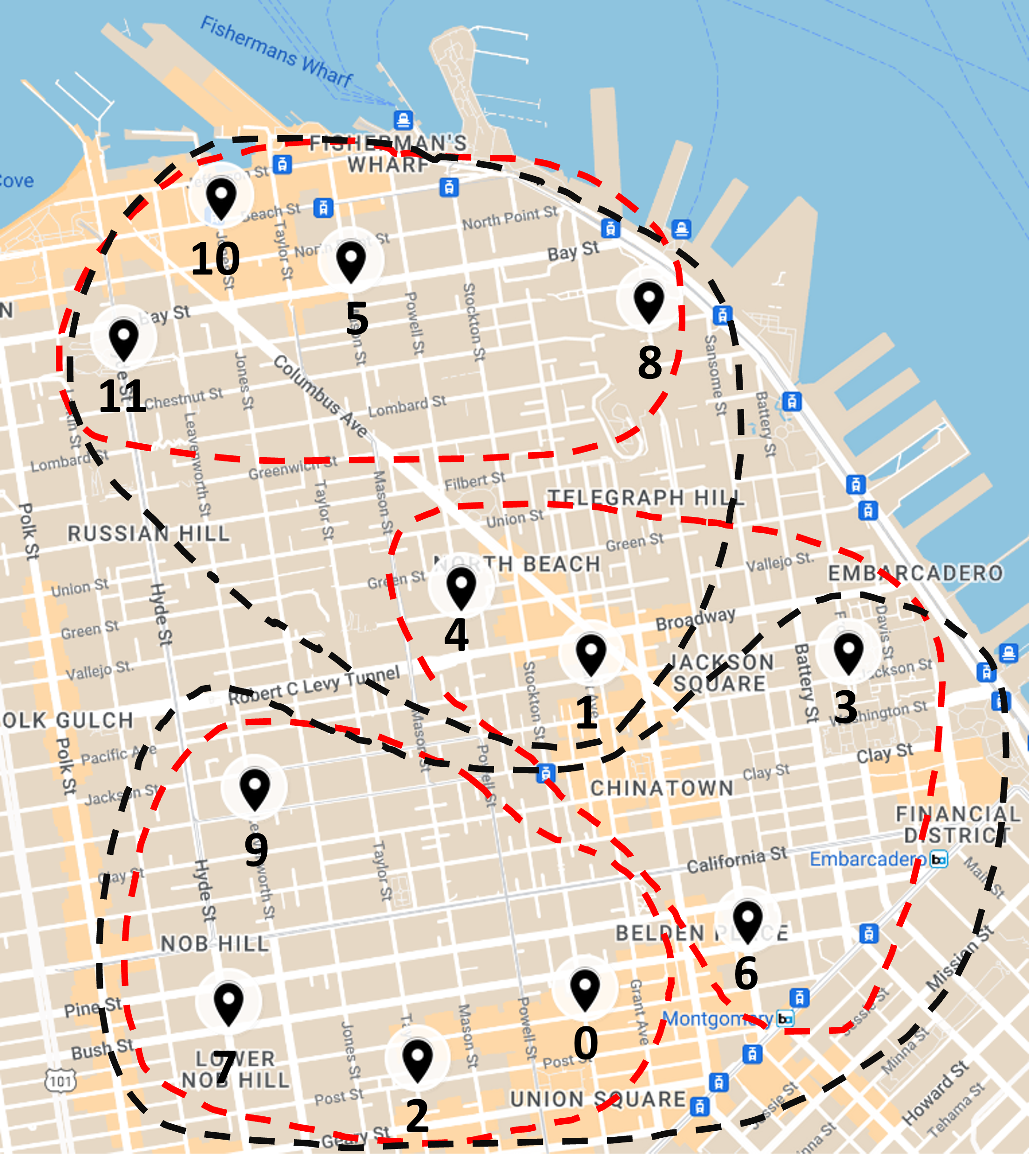
Figure 1: Twelve intersections in the central district of the San Francisco police department.

IV-A Single-Robot Patrolling

First we study single-robot patrolling. We begin by substantiating the claim that RoSSO is more computationally efficient than the existing software [24]. We compare with their MATLAB implementation that leverages the general-purpose constrained nonlinear programming solver fmincon. Table I contains the comparison data averaged over 10 runs. The SG formulation is excluded from the comparison because [24] does not appear to yield meaningful results for that formulation. The wall times are comparable for the MHT formulation, but the optimized objective function value for [24] is noticeably worse due to their inclusion of the reversibility constraint on the MC. We see a dramatic speedup using RoSSO for the RTE formulation. We expect the performance improvements of RoSSO to increase on GPU/TPU hardware due to implementation in JAX.

TABLE I: Computational efficiency comparison between RoSSO and [24] averaged over 10 random initializations.

		MHT	RTE
RoSSO	Avg. Wall Time [s]	1.14	11.5
	Avg. Obj. Fun. Value	23.7	5.00
[24] (MATLAB)	Avg. Wall Time [s]	0.81	409
	Avg. Obj. Fun. Value	44.8	5.00

Now we compare the MC metrics presented in Section II. Fig. 2 shows the best results obtained from running RoSSO for the MHT, SG, and RTE formulations with 100 random initializations. The corresponding objective function and penalty values are given in Table III. $\alpha=1$ was used in the penalty term of the objective function. The stopping criterion for the optimization was a mean relative change in objective function value less than 0.01 over 10 successive iterations. The RMSprop gradient-based optimization algorithm was found empirically to be effective on these problems [22]. We also discovered that convergence occurs more quickly for the SG formulation if the mean of the lowest 4 capture probabilities is maximized rather than just the lowest. The computational efficiency data is given in Table II and shows that the RTE formulation is much more computationally expensive than the other formulations.

We see in Fig. 2(a) that the MHT strategy is asymmetric and sparse. This strategy can be thought of as a cycle over the graph with some probability of staying at intersections 0 and 3 for multiple consecutive time periods. This allows the strategy to meet the stationary distribution constraint. A robot patroller using this strategy will be quite predictable. The RTE strategy shown in Fig. 2(b) is asymmetric and dense. This strategy resembles a uniform random walk that meets the stationary distribution constraint. Clearly, a robot following this patrol strategy will be hard to predict. Note that the truncation accuracy was set to $\eta=0.1$ as in [10]. This corresponds to $K_{\eta}=2295$ in Eq. (11) and explains the slow computation shown in Table II. The SG strategy shown in Fig. 2(c) is asymmetric and a middle ground in terms of sparsity. This strategy has features similar to both the MHT and the RTE strategies. The vector of attack durations $\boldsymbol{\tau}=9\cdot\mbox{1}_{n}$ was chosen as the worst-case uniform attack duration scenario with a nonzero capture probability.

TABLE II: Averaged computational efficiency data for RoSSO.

	MHT	RTE	SG	SG Co-Opt	Multi-SG ($R=2$)	Multi-SG ($R=3$)	Part. Multi-SG ($R=2$)	Part. Multi-SG ($R=3$)
Avg. Wall Time [s]	1.14	11.5	3.07	17.2	10.9	174	1.81	1.72
Avg. No. of Iterations	460	12	2103	2697	2577	1431	444	209
Avg. Speed [iter/s]	405	1.04	685	156	237	8.24	245	122

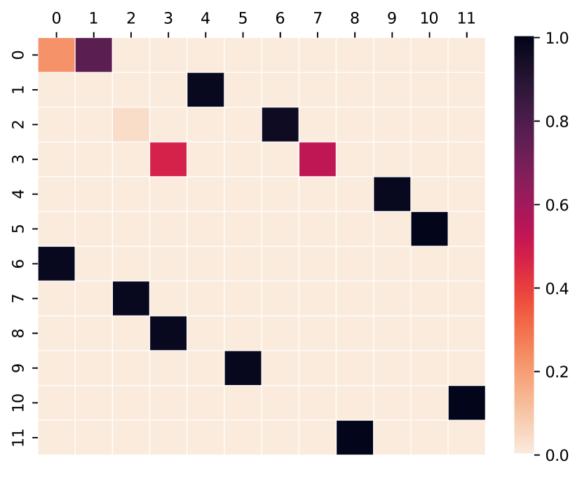
(a) MHT, Section II-C

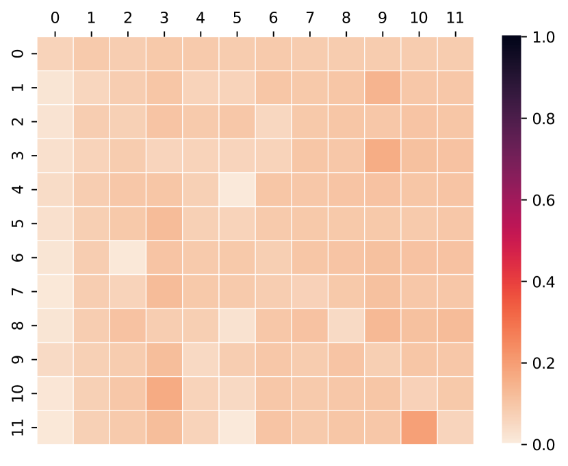
(b) RTE, Section II-D

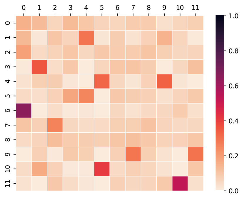
(c) SG, Section II-E

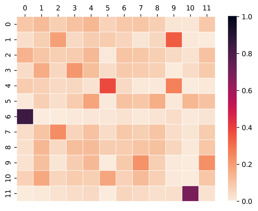
(d) SG Co-Opt, Section III-C

Figure 2: Heatmaps of optimized single-robot patrol strategies for San Francisco graph from RoSSO.

Now we consider the simultaneous optimization of defense placement and patrol strategy in the SG formulation as described in Section III-C. The defense budget $B=9\times 12=108$ to compare with the results in Fig. 2(c). Fig. 2(d) displays the best resulting patrol strategy from 100 random initializations. The corresponding vector of attack durations $\boldsymbol{\tau}=\setcounter{MaxMatrixCols}{12}\begin{bmatrix}8&6&11&10&6&10&9&10&11&9&10&8\end{bmatrix}^{\top}$. Note that this nonuniform choice of $\boldsymbol{\tau}$ leads to a relative increase of 5% in SG capture probability as shown in Table III. The drawback is increased computational expense as shown in Table II.

Table III gives the values of all three metrics for each of the optimized strategies shown in Fig. 2. Recall that the aim is to minimize $J_{\textup{MHT}}$, Penalty and maximize $J_{\textup{RTE}},J_{\textup{SG}}$. We see that the MHT strategy performs poorly when evaluated by the RTE and SG metrics. This is due to the sparsity of the strategy and the long intervals between departure and arrival for certain pairs of nodes, respectively. The RTE strategy suffers on the MHT metric due to slow traversal of the patrol area. The SG strategy and the co-optimized SG strategy perform reasonably well on all metrics. The $J_{\textup{MHT}}$ values 48.8 and 47.9 are acceptable considering that the optimal value is 44.8 when including the reversibility constraint.

TABLE III: Evaluation of the optimized strategies from Fig. 2 by each metric.

	Fig. 2(a)	Fig. 2(b)	Fig. 2(c)	Fig. 2(d)
$J_{\textup{MHT}}$	21.2	58.1	48.8	47.9
$J_{\textup{RTE}}$	2.10	5.13	4.71	4.64
$J_{\textup{SG}}$	$1.17\mathrm{e}{-8}$	$1.97\mathrm{e}{-2}$	$9.75\mathrm{e}{-2}$	$10.2\mathrm{e}{-2}$
Penalty	$9.94\mathrm{e}{-3}$	$2.97\mathrm{e}{-2}$	$5.13\mathrm{e}{-3}$	$4.70\mathrm{e}{-3}$

IV-B Multi-Robot Patrolling

Here we compare our proposed multi-robot SG formulation from Section III-D with a partitioning approach. We focus on the SG metric due to the aforementioned balanced nature of the SG strategies. We obtained better results for this formulation by maximizing just the lowest capture probability. The other parameters are unchanged from the single-robot results. Fig. 3 shows the best optimized strategies from 10 random initializations for teams of robot patrollers. Figs. 3(a), 3(b) contain the $R=2$ results, and Figs. 3(c), 3(d), 3(e) contain the $R=3$ results. We can see that the optimized strategies naturally divide up the graph and focus each robot’s attention on a subset of the intersections. We emphasize that this is purely emergent behavior; no restrictions were imposed beyond MC validity and the stationary distribution penalty given in Eq. (8). For example in the $R=2$ results, the first robot is biased towards intersections 0-4, 6, and 7 while the second robot is biased towards intersections 5 and 8-11. Examining the map in Fig. 1, we see that this is a reasonable division of labor.

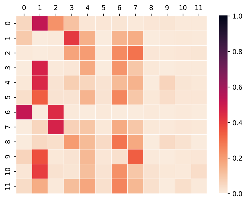
(a) $R=2$,
$J_{\textup{SGM}}=0.167$,
$\text{penalty}=0.664$

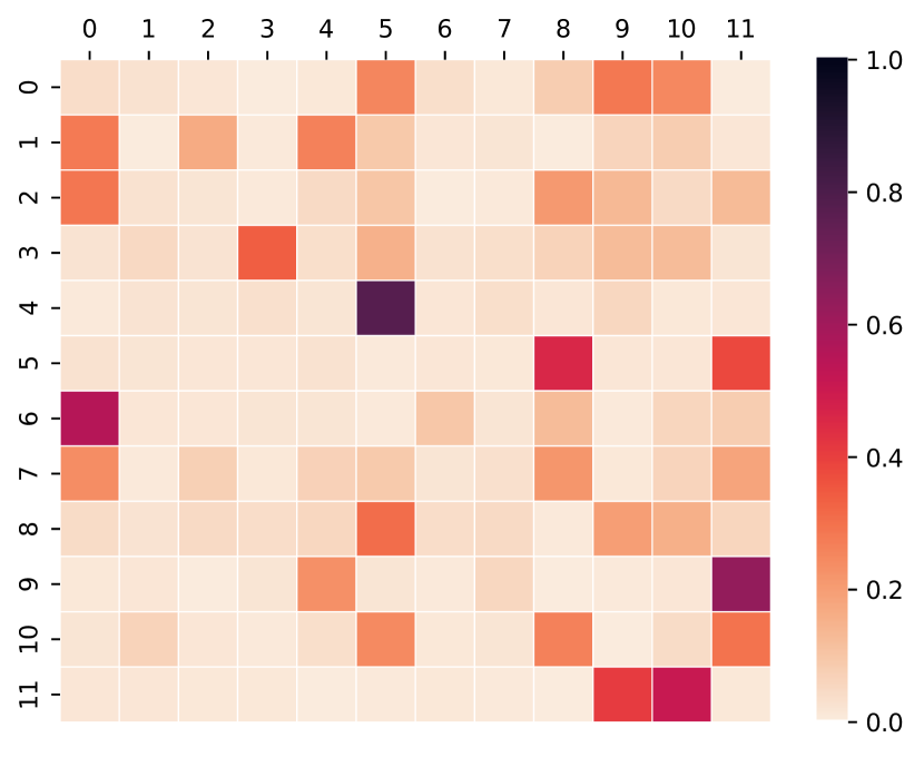
(b) $R=2$,
$J_{\textup{SGM}}=0.167$,
$\text{penalty}=0.664$

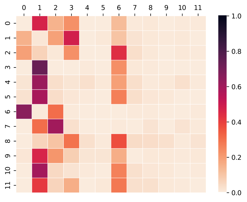
(c) $R=3$,
$J_{\textup{SGM}}=0.278$,
$\text{penalty}=0.207$

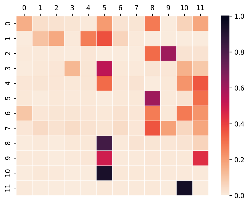
(d) $R=3$,
$J_{\textup{SGM}}=0.278$,
$\text{penalty}=0.207$

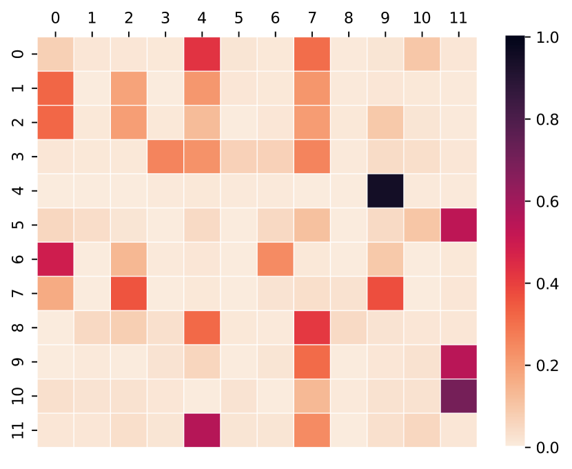
(e) $R=3$,
$J_{\textup{SGM}}=0.278$,
$\text{penalty}=0.207$

Figure 3: Heatmaps of SG-optimized robot team patrol strategies for San Francisco graph from RoSSO, Section III-D.

The computational efficiency data in Table II shows the expected drastic slowdown as the number of robots $R$ increases.

We compare with a prescribed partition approach. The partitions are chosen a priori as shown in Fig. 1. Fig. 4 shows the best optimized strategies from 10 random initializations for single-robot patrollers confined to partitions of the graph. Figs. 4(a), 4(b) contain the $R=2$ results, and Figs. 4(c), 4(d), 4(e) contain the $R=3$ results. Notice that the capture probabilities are higher with this approach. However, this depends on appropriate partitioning which is a nontrivial problem for large graphs. Additionally, the set of possible strategies when using a partitioning approach is a subset of the strategies that can be described by the un-partitioned MCs. With a sufficient number of random initializations, we expect the un-partitioned approach to achieve equivalent or better performance.

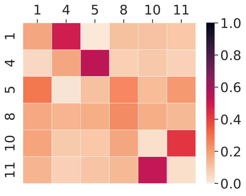
(a) $R=2$,
$J_{\textup{SG}}=0.307$,
$\text{penalty}=1.26\mathrm{e}{-2}$

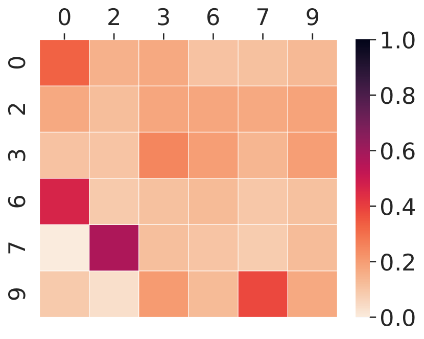
(b) $R=2$,
$J_{\textup{SG}}=0.260$,
$\text{penalty}=7.43\mathrm{e}{-3}$

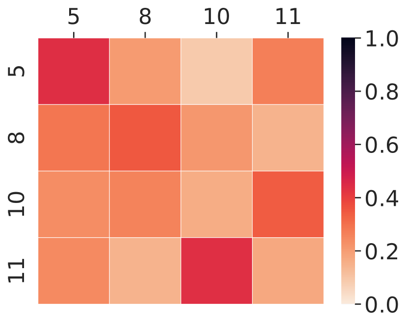
(c) $R=3$,
$J_{\textup{SG}}=0.488$,
$\text{penalty}=1.06\mathrm{e}{-2}$

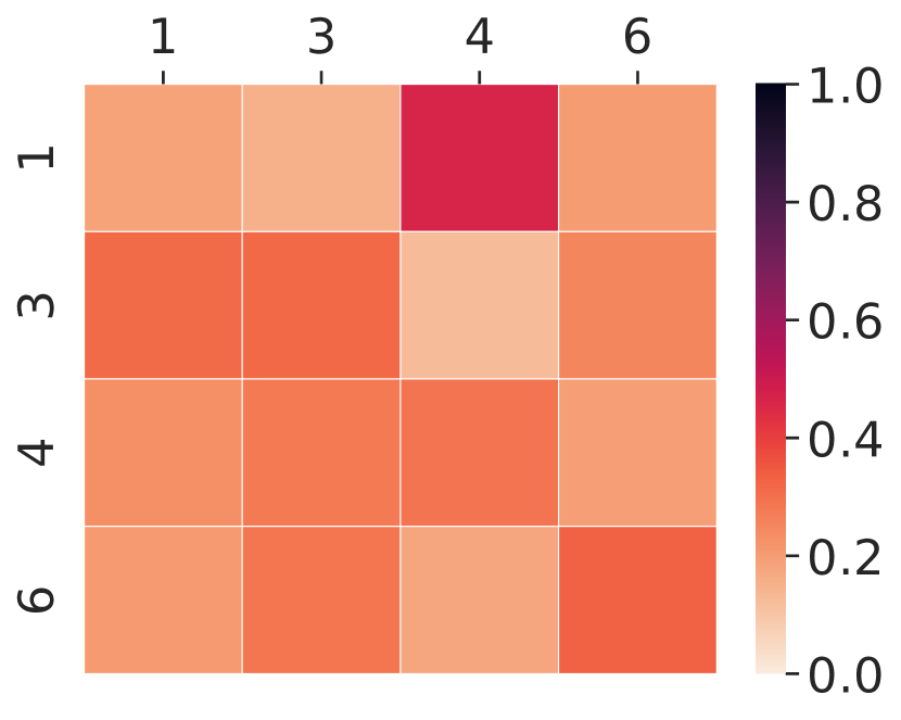
(d) $R=3$,
$J_{\textup{SG}}=0.416$,
$\text{penalty}=2.06\mathrm{e}{-3}$

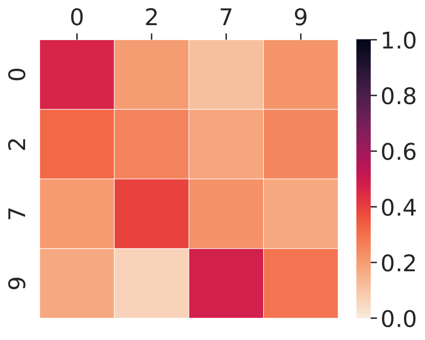
(e) $R=3$,
$J_{\textup{SG}}=0.514$,
$\text{penalty}=1.59\mathrm{e}{-2}$

Figure 4: Heatmaps of SG-optimized robot team patrol strategies for partitioned San Francisco graph from RoSSO.

The computational efficiency data in Table II shows the appeal of the partitioning approach. Again, we emphasize that additional computation time would be needed for choosing appropriate partitions in a large graph. We also remark that the first iteration of optimization using RoSSO can take noticeably longer than following iterations due to accelerated linear algebra compilation. This can slightly skew the average speed figures presented in Table II when the number of iterations is small.

V Conclusions

RoSSO is a valuable tool for enabling MC optimization over a realistic graph with travel times and varying node priority. Using RoSSO, we conducted a case study on the San Francisco crime graph that identified the SG metric as a good choice for generating patrol strategies that balance movement speed and unpredictability. Focusing on the SG formulation, we proposed a novel greedy algorithm for the design problem of co-optimizing defense budget allocation and patrol strategy. On the multi-robot front, we proposed a novel SG formulation and leveraged the computational efficiency of RoSSO to optimize it. We compared against a graph partitioning approach and discovered that appropriately chosen partitions can narrow the state space and lead to effective strategies with fewer random initializations and less computational expense per initialization. In future, we aim to achieve further speedup via parallelized computation on GPU/TPU hardware. Additionally, the JAX community has developed several reinforcement learning libraries that we intend to explore for robotic surveillance applications.

Appendix

Here we define the stationary distribution and first hitting times of an MC. The MC $P$ is irreducible if every node is reachable from every other node. An irreducible MC $P$ has a unique nonnegative stationary distribution $\boldsymbol{\pi}\in\mathbb{R}^{n}$ that satisfies $\boldsymbol{\pi}^{\top}P=\boldsymbol{\pi}^{\top}$, $\boldsymbol{\pi}^{\top}\mbox{1}_{n}=1$. The stationary distribution represents the fraction of the robot’s time spent at each node in the graph. Let $X_{k}\in\{1,\ldots,n\}$ be the state of an MC at time period $k$. The first hitting time, $T_{ij}$, is a random variable representing the duration between the robot’s departure from waypoint $i$ and its first arrival at waypoint $j$, i.e., $T_{ij}=\min\{k\mid X_{0}=i,X_{k}=j,k\geq 1\}$. The first hitting time probability matrices $F_{k}$ can be defined wherein $F_{k}(i,j)=\mathbb{P}(T_{ij}=k)$. Recursions for computing $F_{k}$ are presented in [10]. For graphs with homogeneous travel times, we have the following where $F_{1}=P$:

$$\textup{vec}(F_{k})=(I_{n}\otimes P)(I_{n^{2}}-\textup{diag}(\textup{vec}(I_{n})))\textup{vec}(F_{k-1}),$$ (10)

For graphs with heterogeneous travel times, we have:

$$\textup{vec}(F_{k})=\textup{vec}\bigl{(}P\circ\bm{1}_{\{k\mbox{1}_{n}\mbox{1}_{n}^{\top}=W\}}\bigr{)}$$ (11)

$$+\sum\nolimits_{i=1}^{n}\sum\nolimits_{j=1}^{n}P(i,j)\bigl{(}E_{j}\otimes\bm{e}_{i}\bm{e}_{j}^{\top}\bigr{)}\textup{vec}\bigl{(}F_{k-w_{ij}}\bigr{)},$$

where $\bm{1}_{\{\cdot\}}$ is the indicator function, $E_{j}=\textup{diag}(\mbox{1}_{n}-\bm{e}_{j})$, and $F_{k}=\mbox{0}_{n\times n}$ for all $k\leq 0$.

References

- [1] N. Agmon, C.-L. Fok, Y. Emaliah, P. Stone, C. Julien, and S. Vishwanath. On coordination in practical multi-robot patrol. In 2012 IEEE International Conference on Robotics and Automation, pages 650–656. IEEE, 2012.
- [2] N. Agmon, S. Kraus, and G. A. Kaminka. Multi-robot perimeter patrol in adversarial settings. In IEEE Int. Conf. on Robotics and Automation, pages 2339–2345, Pasadena, USA, May 2008.
- [3] T. Alam, M. M. Rahman, P. Carrillo, L. Bobadilla, and B. Rapp. Stochastic multi-robot patrolling with limited visibility. Journal of Intelligent & Robotic Systems, 97(2):411–429, 2020.
- [4] S. Alamdari, E. Fata, and S. L. Smith. Persistent monitoring in discrete environments: Minimizing the maximum weighted latency between observations. International Journal of Robotics Research, 33(1):138–154, 2014.
- [5] I. Babuschkin, K. Baumli, A. Bell, S. Bhupatiraju, J. Bruce, P. Buchlovsky, D. Budden, T. Cai, A. Clark, I. Danihelka, A. Dedieu, C. Fantacci, J. Godwin, C. Jones, R. Hemsley, T. Hennigan, M. Hessel, S. Hou, S. Kapturowski, T. Keck, I. Kemaev, M. King, M. Kunesch, L. Martens, H. Merzic, V. Mikulik, T. Norman, G. Papamakarios, J. Quan, R. Ring, F. Ruiz, A. Sanchez, L. Sartran, R. Schneider, E. Sezener, S. Spencer, S. Srinivasan, M. Stanojević, W. Stokowiec, L. Wang, G. Zhou, and F. Viola. The DeepMind JAX Ecosystem, 2020.
- [6] S. Boyd, P. Diaconis, and L. Xiao. Fastest mixing Markov chain on a graph. SIAM Review, 46(4):667–689, 2004.
- [7] J. Bradbury, R. Frostig, P. Hawkins, M. J. Johnson, C. Leary, D. Maclaurin, G. Necula, A. Paszke, J. VanderPlas, S. Wanderman-Milne, and Q. Zhang. JAX: composable transformations of Python+NumPy programs, 2018.
- [8] Y. Chevaleyre. Theoretical analysis of the multi-agent patrolling problem. In IEEE/WIC/ACM Int. Conf. on Intelligent Agent Technology, pages 302–308, Beijing, China, September 2004.
- [9] G. Diaz-García, F. Bullo, and J. R. Marden. Distributed Markov chain-based strategies for multi-agent robotic surveillance. IEEE Control Systems Letters, 7:2527–2532, 2023.
- [10] X. Duan, M. George, and F. Bullo. Markov chains with maximum return time entropy for robotic surveillance. IEEE Transactions on Automatic Control, 65(1):72–86, 2020.
- [11] X. Duan, D. Paccagnan, and F. Bullo. Stochastic strategies for robotic surveillance as Stackelberg games. IEEE Transactions on Control of Network Systems, 8(2):769–780, 2021.
- [12] M. George, S. Jafarpour, and F. Bullo. Markov chains with maximum entropy for robotic surveillance. IEEE Transactions on Automatic Control, 64(4):1566–1580, 2019.
- [13] J. Grace and J. Baillieul. Stochastic strategies for autonomous robotic surveillance. In IEEE Conf. on Decision and Control and European Control Conference, pages 2200–2205, Seville, Spain, December 2005.
- [14] J. P. Hespanha, H. J. Kim, and S. S. Sastry. Multiple-agent probabilistic pursuit-evasion games. Technical report, Electrical Engineering and Computer Science, University of California at Berkeley, August 1999. Available at http://www.ece.ucsb.edu/ hespanha/published.
- [15] S. Hosseinalipour, A. Rahmati, H. Dai, et al. Energy-aware stochastic uav-assisted surveillance. IEEE Transactions on Wireless Communications, 20(5):2820–2837, 2020.
- [16] C. Hughes and Y. John. Rosso. https://github.com/conhugh/RoSSO, 2023.
- [17] Y. John, G. Diaz-Garcia, X. Duan, J. R. Marden, and F. Bullo. A stochastic surveillance stackelberg game: Co-optimizing defense placement and patrol strategy. arXiv preprint arXiv:2308.14714, 2023.
- [18] S. M. LaValle, D. Lin, L. J. Guibas, J.-C. Latombe, and R. Motwani. Finding an unpredictable target in a workspace with obstacles. In Proceedings of International Conference on Robotics and Automation, volume 1, pages 737–742. IEEE, 1997.
- [19] R. Patel, P. Agharkar, and F. Bullo. Robotic surveillance and Markov chains with minimal weighted Kemeny constant. IEEE Transactions on Automatic Control, 60(12):3156–3167, 2015.
- [20] R. Patel, A. Carron, and F. Bullo. The hitting time of multiple random walks. SIAM Journal on Matrix Analysis and Applications, 37(3):933–954, 2016.
- [21] P. E. Rybski, N. P. Papanikolopoulos, S. A. Stoeter, D. G. Krantz, K. B. Yesin, M. Gini, R. Voyles, D. F. Hougen, B. Nelson, and M. D. Erickson. Enlisting rangers and scouts for reconnaissance and surveillance. IEEE Robotics & Automation Magazine, 7(4):14–24, 2000.
- [22] T. Tieleman and G. Hinton. Lecture 6.5-rmsprop: Divide the gradient by a running average of its recent magnitude, 2012. COURSERA: Neural networks for machine learning.
- [23] R. von Mises and H. Pollaczek-Geiringer. Praktische verfahren der gleichungsauflösung. ZAMM-Journal of Applied Mathematics and Mechanics/Zeitschrift für Angewandte Mathematik und Mechanik, 9(1):58–77, 1929.
- [24] H. Wang. Robotic surveillance package. https://github.com/HanWang99/RoboSurv, November 2019. A Matlab and Julia library for the computation of robotic surveillance strategies, licensed under CC BY-NC-SA 4.0.