CoCA: Fusing position embedding with Collinear Constrained Attention for fine-tuning free context window extending

Abstract

Self-attention and position embedding are two key modules in Transformer based LLMs. The potential relationship among them are far from well studied, especially for context window extending. In this paper, we introduce collinear constrained relationship to fuse RoPE and self-attention, and name it as Collinear Constrained Attention (CoCA). We’ve analyzed the computational and spatial complexity of CoCA and have determined that it adds only minimal additional overhead compared to the original Transformer-based models. We provide an efficient implementation of CoCA, and make it drop-in replacement for any existing position embedding and attention modules in Transformer based models. Experiments show that CoCA performs extraordinary well on context window extending. For instance, a CoCA based GPT model trained with 512 context length can extend the context window up to 8K without perplexity diverging. This indicates more than 16x context window extending without any fine-tuning. Our code is released here: https://github.com/codefuse-ai/Collinear-Constrained-Attention

1 Introduction

In the seminal work of Transformer  (Vaswani et al., 2017), it claims the ability of “extrapolating to sequence lengths longer than the ones encountered during training”. This was an ideal hypothesis but actually not work in practice for original Transformer. Hence, there are a bunch of follow-up works generally referred as position embedding, which investigates the ability of large language models (LLMs) that are trained with position embedding in the range of $[0,T-1]$ to effectively extend the testing sequence longer than $T$ ($\geq T$).

Many subsequent researches are dedicated on this topic, such as (Press et al., 2021; Sun et al., 2022; Chi et al., 2022; Chen et al., 2023; Tworkowski et al., 2023; bloc97, 2023). They can be generally divided into three categories. First, different methods such as ALiBi (Press et al., 2021), Xpos (Sun et al., 2022) and KERPLE (Chi et al., 2022) are integrated into the pre-training stage to handle context extrapolation problem. For instance, ALiBi introduced a relative offset based linear bias into the attention matrix replacing original position embedding to realize extrapolation. These methods add certain kinds of local hypothesis to context tokens, which suffers from the defect to capture long-range dependence. Second, techniques are introduced into the fine-tuning stage for context extending, which includes PI (Chen et al., 2023) and FoT (Tworkowski et al., 2023). For instance, FoT introduces a key-value network to handle long context. These kinds of methods work well for off-the-shelf models, but they are not essential solution for the problem. And more important, it lacks of theoretic guarantee for the generalization capability to cover different aspects of pre-training knowledge. Third, some tricks are introduced into a training and fine-tuning free manner for context extrapolation. For instance, NTK-aware Scaled RoPE (bloc97, 2023) adopts neural tangent kernel to transfer the extrapolation problem with an interpolation methods, with limited code changes during inference. The training/fine-tuning free based methods suffer from very limited context window extending ratio. For instance, NTK-aware method can only extend the training context window about 4 to 8 times of original, and without guarantee of performance. This far from practical requirement.

We conducted a series of analysis for aforementioned methods, especially for those based on widely used rotary position embedding (RoPE) Su et al. (2021). As is known, RoPE is a relative position encoding technique designed based on the relative angular difference between the query ($Q$) and key ($K$), while there are latent relationship between $Q$ and $K$ in the self-attention, since the two matrices are directly multiplied within the softmax function. We demonstrate the incorrect initialization of the angle between $Q$ and $K$ in RoPE yields undesirable behavior around context window boundary, and further makes it perform poor for context extrapolation. This urges us to combine position embedding and self-attention together for systematic modeling to alleviate the undesirable behavior issues on context boundary.

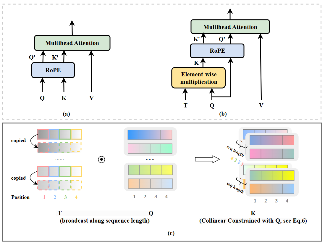
In this paper, we handle the aforementioned issue fusing RoPE with self-attention mechanism, and propose the novel Collinear Constrained Attention(CoCA). Figure 1 illustrates the architecture of CoCA. Specifically, by enforcing the colinear constraint between the query and key (i.e., the initial angle between them is 0), we achieve excellent results in fine-tuning free context extrapolation. For instance, a GPT model trained only with a context window size of 512 tokens. Without any fine-tuning, it can extrapolate to sequences up to 8k or even longer without perplexity diverging. The model also performs better in capturing long-range dependence according to passkey evaluation when combining the NTK-aware method. The main contributions can be summarized as follows:

Figure 1: Architecture comparison between self-attention and Collinear Constrained Attention (CoCA). (a) Original self-attention and RoPE; (b) CoCA; (c) Q, T and V are generated by projection matrices same as original self-attention. T is half-size of Q, and K is generated based on Q and T with the collinear constraint.

• We reveal undesirable context boundary behavior when lacking of modeling the relationship between position embedding and self-attention, and thus propose to fuse them together with colinear constraints attention (CoCA) for fine-tuning free long context window extending.

• Extensive experiments show that without fine-tuning, GPT model trained with CoCA can extend context window length 16 times (from 512 to 8K) without perplexity diverging.

• CoCA also shows the capability to capture long-range dependence in the passkey evaluation. For instance, it can maintain a passkey accuracy of $60\%+$ even when extrapolating to 16 times of its training context length. Which is $20\%+$ higher than original self-attention with RoPE, and $50\%+$ higher than ALibi.

• We make theoretic analysis of the computing and space complexity of CoCA, which shows it adds relative smaller overhead to the original Transformer models. We also provide an efficient CoCA implementation, which demonstrates comparable training performance to the original Transformer models.

We have made a full implementation of CoCA open-sourced: https://github.com/codefuse-ai/Collinear-Constrained-Attention.

2 Method

2.1 Background: Rotary Position Embedding (RoPE)

Positional encoding plays a important role in Transformer models since it represents the order of inputs. We consider Rotary Position Embedding(RoPE) (Su et al., 2021) here, which is a positional encoding method used by LLaMA model (Touvron et al., 2023), GPT-NeoX (Black et al., 2022), etc. Suppose the position index is an interger $n\in[0,c)$ and the corresponding input vector ${\mathbf{x}}:=(x_{0},x_{1},...,x_{d-1})$, where $d$ represents the dimension of the attention head and always even. RoPE defines a vector-valued complex function $f({\mathbf{x}},n)$ as follows:

$$f({\mathbf{x}},n)=((x_{0}+ix_{d/2})e^{in\theta_{0}},(x_{1}+ix_{1+d/2})e^{in\theta_{1}},...,(x_{d/2-1}+ix_{d-1})e^{in\theta_{d/2-1}})$$ (1)

where $i:=\sqrt{-1}$ is the imaginary unit and $\theta_{j}=10000^{-2j/d}$. Attention score after applying RoPE is:

$$a(m,n) =\text{Re}(\langle f({\mathbf{q}},m),f({\mathbf{k}},n)\rangle)$$ (2)

$$=\text{Re}\left[\sum_{j=0}^{d/2-1}(q_{j}+iq_{j+d/2})(k_{j}-ik_{j+d/2})e^{i(m-n)\theta_{j}}\right]$$

$$=\sum_{j=0}^{d/2-1}((q_{j}k_{j}+q_{j+d/2}k_{j+d/2})\text{cos}((m-n)\theta_{j})$$

$$\ \ \ \ +(q_{j}k_{j+d/2}-q_{j+d/2}k_{j})\text{sin}((m-n)\theta_{j}))$$

$$:=a(m-n)$$

Here, ${\mathbf{q}}$ and ${\mathbf{k}}$ denote the query and key vectors for a particular attention head. The attention score $a(m-n)$ is only dependent on relative position $(m-n)$. It is a beautiful design that works with the attention mechanism to achieve relative positional encoding in the way of absolute positional encoding. This feature renders RoPE more efficient than other position encoding techniques and is inherently compatible with linear attentions.

2.2 Long-term decay of RoPE

As studied by (Su et al., 2021) before, RoPE has the characteristic of long-term decay:

$$|a(s)| =\Bigg{|}\text{Re}\left[\sum_{j=0}^{d/2-1}h_{j}e^{is\theta_{j}}\right]\Bigg{|}$$ (3)

$$\leq(\max_{i}|h_{i+1}-h_{i}|)\sum_{j=0}^{d/2-1}|S_{j+1}|$$

where $h_{j}:=(q_{j}+iq_{j+d/2})(k_{j}-ik_{j+d/2})$ and $S_{j}:=\sum_{k=0}^{j-1}e^{is\theta_{k}}$. Since the value of $\sum_{j=0}^{d/2-1}|S_{j+1}|$ decays with the relative distance $s$, the attention score decays either.

This is consistent with human understanding of language modeling.

We claim that we could get a much more stronger one with collinear constraint later.

2.3 Anomalous behavior between RoPE and attention matrices

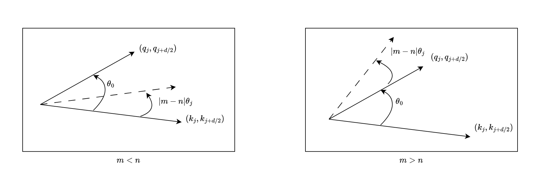
In Equation 2, we represent the attention score after applying RoPE as $a(m-n)$, mathematically, it can be visualized as the inner-product of two complex number after a rotation for any individual $j\in[0,d/2]$, just like Figure 2.

It intuitively make sense, since position distance can be modeling as one kind of order and the inner-product of two complex number changes with the rotation angle $(m-n)\theta$.

However, we will show that it is not a qualified order with a technical deficiency.

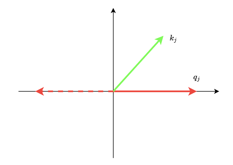
For simplicity, we consider bidirectional models first, such as Bert (Devlin et al., 2019) and GLM (Du et al., 2021), etc. As shown in Figure 2, for any pair of ${\mathbf{q}}_{j}$ and ${\mathbf{k}}_{j}$, without loss of generality, we suppose that there is an angle $\theta_{0}$ which is smaller than $\pi$ to rotate counterclockwise from ${\mathbf{k}}_{j}$ to ${\mathbf{q}}_{j}$ in the complex plane, then we have two possible conditions of their position indices(while $=$ is ordinary).

• When $m>n$, shown as the right part of Figure 2, it’s the order preserving one what we want. Since the attention score decreases when the position distance increase(until they rotate out of $\pi$, we will discuss this part in Appendix A).

• However, when $m<n$, shown as the left part of Figure 2, the anomalous behavior which breaks the order at closest tokens with the number of $\theta_{0}/\theta_{j}$. More terribly, it always accompanies the model whether applying PI (Chen et al., 2023) or NTK-aware Scaled RoPE (bloc97, 2023). Since we could only survive by cutting tail but not head.

Figure 2: Broken of order in bidirectional models. The inner-product of ${\mathbf{q}}_{j}$ and ${\mathbf{k}}_{j}$ is based on the relative angle between them. Left: when $|m-n|\theta_{j}<\theta_{0}$, the relative angle between ${\mathbf{q}}_{j}$ and ${\mathbf{k}}_{j}$ will decrease with $|m-n|$, which means closest tokens may get smaller attention scores. (We use ’may’ here since the attention score is the sum of $d/2$ inner-products, maybe one of them is insignificant. However, experiments confirmed this significance.). Right: no anomalous behavior.

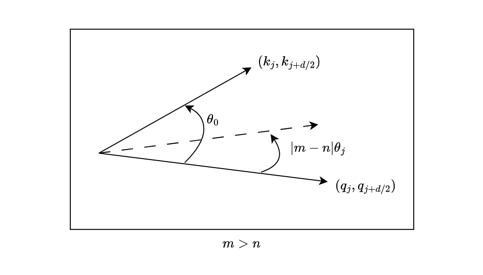
For causal models, it also doomed although $m$ is always larger than $n$. As shown in Figure 3, just for some $j$ when there is an angle $\theta_{0}$ which is smaller than $\pi$ to rotate counterclockwise from ${\mathbf{q}}_{j}$ to ${\mathbf{k}}_{j}$, instead of ${\mathbf{k}}_{j}$ to ${\mathbf{q}}_{j}$.

Figure 3: Broken of order in causal models. Definition of notations are the same as Figure 2, notice that $\theta_{0}$ here is a little different from Figure 2, since it’s counterclockwise from ${\mathbf{q}}_{j}$ to ${\mathbf{k}}_{j}$ here.

2.4 Collinear Constrained Attention(CoCA)

Follow the analysis in Section 2.3, we can naturally deduce the following method: applying a collinear constraint on any pair of ${\mathbf{q}}_{j}$ and ${\mathbf{k}}_{j}$.

Formally, let ${\mathbb{S}}_{N}=\{w_{i}\}_{i=1}^{N}$ be a sequence of $N$ input tokens. The corresponding word embedding of ${\mathbb{S}}_{N}$ is denoted as $\mathbb{E}_{N}=\{{\mathbf{x}}_{i}\}_{i=1}^{N}$, we first get the queries as same as before:

$${\mathbf{q}}_{m}={\bm{W}}_{q}{\mathbf{x}}_{m},\forall m\in[1,N]$$ (4)

Notice that the subscript $m$ here is quite different with $j$ we used in last section, while $m$ here represents the dimension of sequence length and $j$ represents the dimension of hidden size. We abbreviate it here by omitting the dimension of hidden size.

Next, we get the keys in a different way since we have to apply the collinear constraint on it, we get the constraint coefficient first:

$${\mathbf{t}}_{n}={\bm{W}}_{t}{\mathbf{x}}_{n},\forall n\in[1,N]$$ (5)

$$({\mathbf{t}}_{n;[0:d/2-1]},{\mathbf{t}}_{n;[d/2:d-1]})={\mathbf{t}}_{n}$$

$${\mathbf{t}}_{n}=(\frac{{\mathbf{t}}_{n;[0:d/2-1]}+{\mathbf{t}}_{n;[d/2:d-1]}}{2},\frac{{\mathbf{t}}_{n;[0:d/2-1]}+{\mathbf{t}}_{n;[d/2:d-1]}}{2})$$

$${\mathbf{t}}_{n}=\text{Relu}({\mathbf{t}}_{n})$$

it could be regard as folding ${\mathbf{t}}_{n}$ in half along the dimension of hidden size and making a copy.

Secondly, we get the keys as follows:

$${\mathbf{k}}_{n}={\mathbf{Q}}\circ{\mathbf{t}}_{n}=({\mathbf{q}}_{1}\circ{\mathbf{t}}_{n},...,{\mathbf{q}}_{N}\circ{\mathbf{t}}_{n})$$ (6)

where $\circ$ represents Hadamard product. We have to claim that ${\mathbf{k}}_{n}$ here has one more additional dimension than before, since it might bring unimaginable memory pressure(exactly $d$ times large).

Fortunately, we can perfectly handle this with tensor contraction, leading to zero increase in memory consumption(see computational and spatial complexity in Section 3.2).

After this, we can apply RoPE almostly the same as before:

$$f({\mathbf{q}}_{m})=f({\mathbf{q}},m)$$ (7)

$$f({\mathbf{k}}_{n})={\mathbf{Q}}\circ f({\mathbf{t}},n)$$

where $f$ is defined as Equation 1.

Finally, we get the attention score as follows:

$$a(m,n) =\text{Re}(\langle f({\mathbf{q}},m),{\mathbf{q}}_{m}\circ f({\mathbf{t}},n)\rangle)$$ (8)

Thus we have built the collinear constrained attention(CoCA) here. Review that the initial angle $\theta_{0}$ between ${\mathbf{q}}$ and ${\mathbf{k}}$ we defined in Section 2.3, it’s always zero now. No more headaches.

3 Theoretical explanation

3.1 Strong form of Long-term decay

As shown in Section 2.2, RoPE has the characteristic of long-term decay:

$$|a(s)| \leq(\max_{i}|h_{i+1}-h_{i}|)\sum_{j=0}^{d/2-1}|S_{j+1}|$$ (9)

For CoCA, we could deduce a much more stronger one as follows:

$$|a(s)| \leq(\max_{i}|l_{i+1}-l_{i}|)\sum_{j=0}^{d/2-1}|C_{j+1}|$$ (10)

where $l_{j}:=|q_{j}+iq_{j+d/2}||k_{j}+ik_{j+d/2}|$, and $C_{j}:=\sum_{k=0}^{j-1}\text{cos}(s\theta_{j})$. And we always have:

$$|l_{i+1}-l_{i}| \leq|h_{i+1}-h_{i}|$$ (11)

Proof Just notice that, when the initial angle $\theta_{0}$ between ${\mathbf{q}}$ and ${\mathbf{k}}$ is $0$, the attention score can be simplified as:

$$a(s) =\text{Re}\left[\sum_{j=0}^{d/2-1}h_{j}e^{is\theta_{j}}\right]$$ (12)

$$=\sum_{j=0}^{d/2-1}l_{j}\text{cos}(s\theta_{j})$$

Then follow the study of (Su et al., 2021), will easily get the estimation in 10.

For Inequality 11, with triangle inequality, we have:

$$|h_{i+1}-h_{i}|\geq||h_{i+1}|-|h_{i}||$$ (13)

review the definition of $h_{i}=(q_{j}+iq_{j+d/2})(k_{j}-ik_{j+d/2})$, we have:

$$|h_{i+1}-h_{i}| \geq||h_{i+1}|-|h_{i}||$$ (14)

$$=||{\mathbf{q}}_{i+1}{\mathbf{k}}^{*}_{i+1}|-|{\mathbf{q}}_{i}{\mathbf{k}}^{*}_{i}||$$

$$=||{\mathbf{q}}_{i+1}{\mathbf{k}}_{i+1}|-|{\mathbf{q}}_{i}{\mathbf{k}}_{i}||$$

$$=|l_{i+1}-l_{i}|$$

3.2 Computational and spatial complexity

We assign some notations before analysing, see Table 1.

Table 1: Some Notations

Variable	Notation
embedding-size	$V$
sequence length	$n$
number of layers	$L$
number of heads per layer	$h$
dimension of heads	$d$

Table 2: Computational complexity

COMPONENT	Complexity Of Origin Model	Complexity Of CoCA
QK(T)V projection	$3Vndh+3(L-1)nd^{2}h$	$3Vndh+3(L-1)nd^{2}h$
T half	-	$Lndh$
T Relu	-	$Lndh$
QK(T) rotary	$2Lndh$	$2Lndh$
$\text{K}=\text{Q}\circ\text{T}$	-	$Ln^{2}dh$
$\text{QK}^{\text{T}}$	$Ln^{2}dh$	$Ln^{2}dh$
Mask	$Ln^{2}$	$Ln^{2}$
Softmax	$Ln^{2}$	$Ln^{2}$

Since $n\gg d$ in commonly used large language models, we can assert that computational complexity of CoCA is nearly 2 times of origin models with component $\text{K}=\text{Q}\circ\text{T}$ from Table 2, which is worthy by comparing such small cost with its excellent performance.

Apart from computational complexity, another important factor which affects the practicality of one model is spatial complexity. As we pointed out after Equation 6, there will be an unimaginable memory pressure without optimization, see Table 3.

The spatial complexity of component $\text{K}=\text{Q}\circ\text{T}$ will become $d$ times larger than origin model if fully expanded. It’s about $64\sim 256$ times for commonly used models which is unacceptable for practical use.

Table 3: Spatial complexity

COMPONENT	Complexity Of Origin Model	Complexity Of CoCA
QK(T)V projection	$Lnd$	$Lnd$
T half	-	$Lnd$
T Relu	-	$Lnd$
QK(T) rotary	$Lnd$	$Lnd$
$\text{K}=\text{Q}\circ\text{T}$	-	$Ln^{2}d$
$\text{QK}^{\text{T}}$	$Ln^{2}$	$Ln^{2}$
Mask	$Ln^{2}$	$Ln^{2}$
Softmax	$Ln^{2}$	$Ln^{2}$

Before solving this problem, we first get some inspiration by review the computational procedure of $\text{QK}^{\text{T}}$, it could be seen as two steps:

• Element-wise product between Q and K.

• Sum calculation along hidden dimension.

Its spatial complexity will also become $Ln^{2}d$ if fully expanded, only if it contracts along hidden dimension before expanding along sequence length, avoiding full expansion. It also works for $\text{K}=\text{Q}\circ\text{T}$, by combining those two components as follows:

$$\text{QK}^{\text{T}}=\text{Q}(\text{Q}\circ\text{T})^{\text{T}}$$ (15)

Thanks to the work of opt_einsum (a. Smith & Gray, 2018), the optimization of Equation 15 can be easily accomplished for commonly used backends, such as torch and tensorflow.

The memory consumption of CoCA gets zero increase with the optimization of Equation 15.

4 Experiments

We perform experiments on 3 models with exactly the same size, training data and training settings based on GPT-NeoX (Black et al., 2022). The only difference between them is self-attention and position-embedding method. We denote these 3 models as follows:

• Origin: Traditional self-attention structure with RoPE.

• ALibi: Traditional self-attention structure with ALibi.

• CoCA: Collinear Constrained Attention with RoPE.

4.1 Experimental setting

Model Architecture. We modified GPT-NeoX (Black et al., 2022) by incorporating our proposed CoCA method, as detailed in Section 2.4. For a comprehensive understanding of the implementation, please refer to the code provided in our github. We trained a model consisting of 350M parameters. This configuration includes 24 layers with a hidden dimension of 1024 and 16 attention heads. Owing to GPU constraints, we’ve set the maximum sequence length to 512 to further conserve GPUs.

Training Data. Our model is trained on a combination of datasets, including the Pile training dataset (Gao et al., 2020), BookCorpus (Zhu et al., 2015), and the Wikipedia Corpus (Foundation, 2021). Additionally, we incorporated open-source code from GitHub with 1+ stars, which we personally collected. From these datasets, we derived a sample of approximately 50B tokens, maintaining a composition of 75% text and 25% code.

Training Procedure. Our training leverages the next-token prediction objective. The optimization is carried out using AdamW (Loshchilov & Hutter, 2017), set with hyper-parameters $\beta_{1}=0.9$ and $\beta_{2}=0.95$. The learning rate adopts a linear warm-up of 1% of total steps, starting from 1e-7. Subsequently, we adjust the learning rate to 1e-4 and linearly decay it to 1e-5. The training harnesses the computational capabilities of 8 A100 GPUs, with a global batch size of 256 and an accumulation of 2 gradient steps. For the implementation, we deploy PyTorch (Paszke et al., 2019) in tandem with Fully Sharded Data Parallel (Zhao et al., 2023). Our models underwent 2 epochs of training, completing within a span of 72 hours.

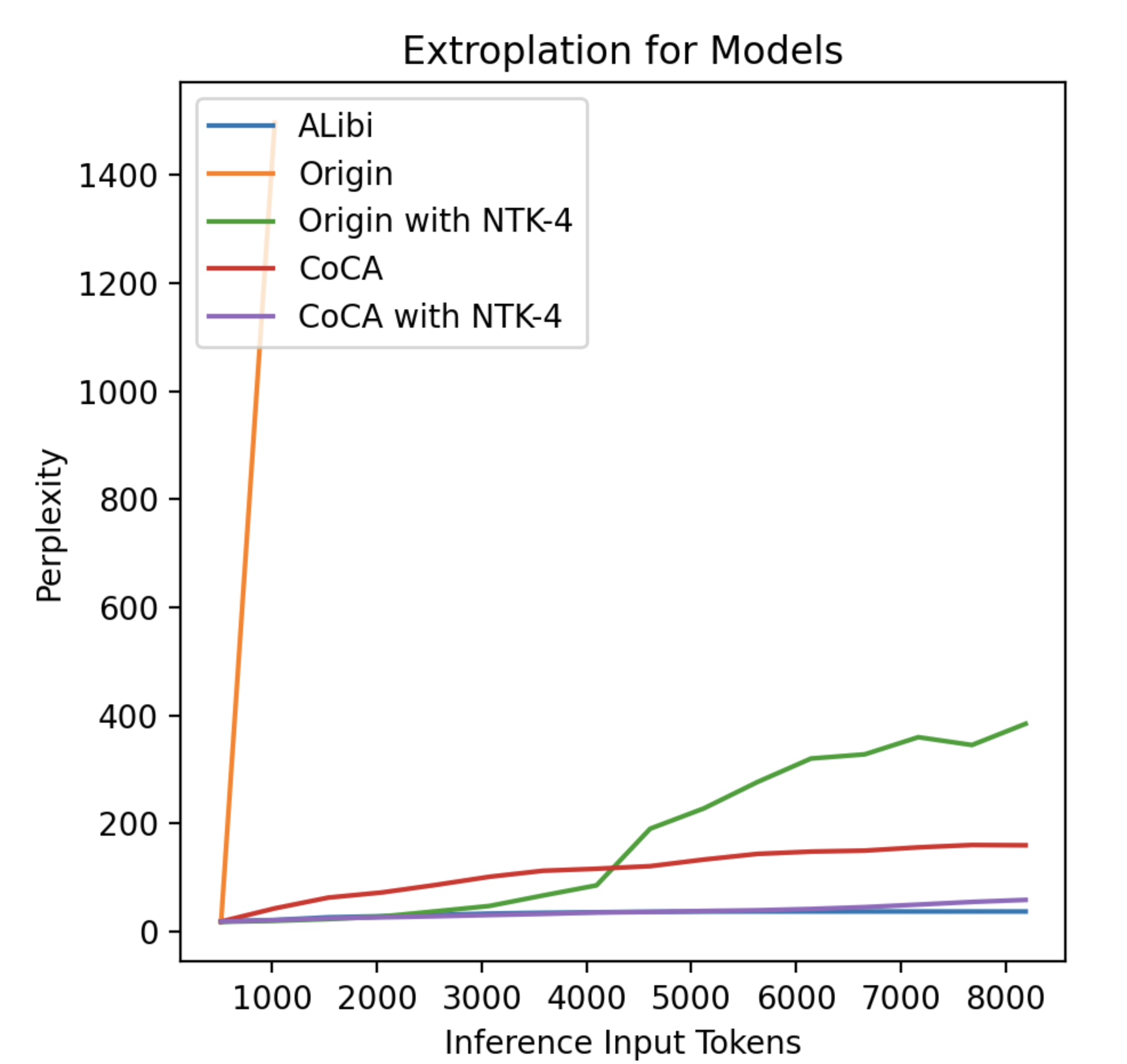
4.2 Long sequence language modeling

We evaluated the long-sequence language modeling prowess of the 3 models. This evaluation was conducted on 100 documents, each possessing at least 8,192 tokens, randomly sourced from the PG-19 dataset (Rae et al., 2019). This methodology follows the approach taken by (Chen et al., 2023). For each test document, we truncated the content to the initial 8,192 tokens. To evaluate perplexity across varied context window sizes, we utilized a sliding window method, in line with (Press et al., 2021), employing a stride S = 256. For fairness, we used exactly the same testing datasets for all 3 models.

Figure 4 illustrates a noteworthy trend: the perplexity of the Origin model rapidly diverges($>1000$) beyond its training length. Conversely, our CoCA model sustains its perplexity at a relatively low plateau even at 16 times its training length.

As a training/fine-tuning free based method, NTK-aware Scaled RoPE (bloc97, 2023) is allowed to be applied in our experiments. However, perplexity of Origin model with scaling factor of 4 for dynamic NTK method is still much more larger than CoCA.

ALibi performs best in perplexity score, and CoCA with dynamic NTK method achieves a level of comparable standards of that.

Figure 4: Sliding window perplexity(S=256) of 100 PG-19 documents. NTK-4 means adopting dynamic NTK method of scaling factor 4 during inference.

4.3 Long-range dependence retrieval

Perplexity is a measure that captures a language model’s proficiency in predicting the next token. However, it doesn’t entirely encompass what we expect from an ideal model. While local attention excels at this task, it often falls short in capturing long-range dependence.

To further evaluate this, we assessed these 3 models using a synthetic evaluation task of passkey retrieval, as proposed by (Mohtashami & Jaggi, 2023). In this task, there is a random passkey hidden in a long document to be identified and retrieved. The prompt format can be seen in LABEL:lst:prompt_passkey.

⬇

There is an important info hidden inside a lot of irrelevant text. Find it and memorize them. I will quiz you about the important information there.

// Reperated fillers.

The grass is green. The sky is blue. The sun is yellow. Here we go. There and back again.

⋮

// Insert PASSKEY here.

The pass key is {PASSKEY}. Remember it. {PASSKEY} is the pass key.

⋮ // Reperated fillers.

The grass is green. The sky is blue. The sun is yellow. Here we go. There and back again.

What is the pass key?

Listing 1: Format of prompt for passkey retrieval. The pass key PASSKEY is randomly generated from 10,000 to 99,999.

For each dataset of sequence length from 256 to 8,192, we first generate a random number of fillers and repeat the filler to make the prompt longer than the individual sequence length at the first time, then insert the passkey into a random position between the fillers. For each dataset of individual sequence length, we make 100 test samples. We check first 64 tokens of model outputs for calculating accuracy. For fairness, we used exactly the same testing datasets for all 3 models.

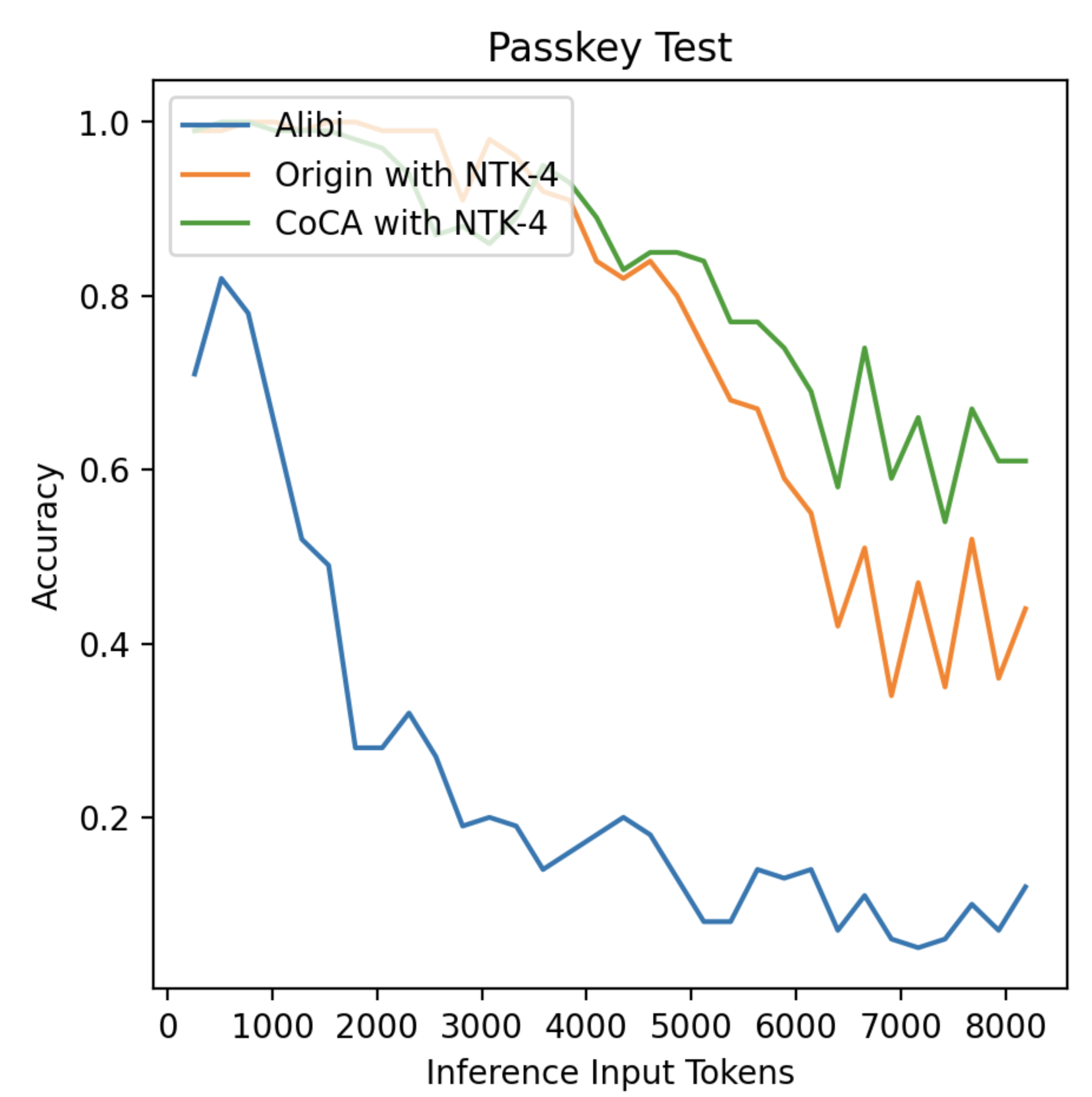
As depicted in Figure 5, methods with local hypothesis such as ALibi demonstrated failures when tested on sequences that were 1 time longer than its training length. In contrast, CoCA consistently exhibited a high degree of accuracy, even when the test sequence length was expanded to 16 times its original training length, $20\%+$ higher than Origin model and $50\%+$ higher than ALibi model. We will delve deeper into some specific interesting instances of CoCA model in Section 4.6.

It’s pertinent to note that we employed the dynamic NTK (no fine-tuning) approach during inference for both CoCA and Origin models in passkey retrieval. Further specifics can be found in Appendix A.

Figure 5: Performance curves of passkey retrieval. NTK-4 means adopting dynamic NTK method of scaling factor 4 during inference.

4.4 Hyper-parameter stability

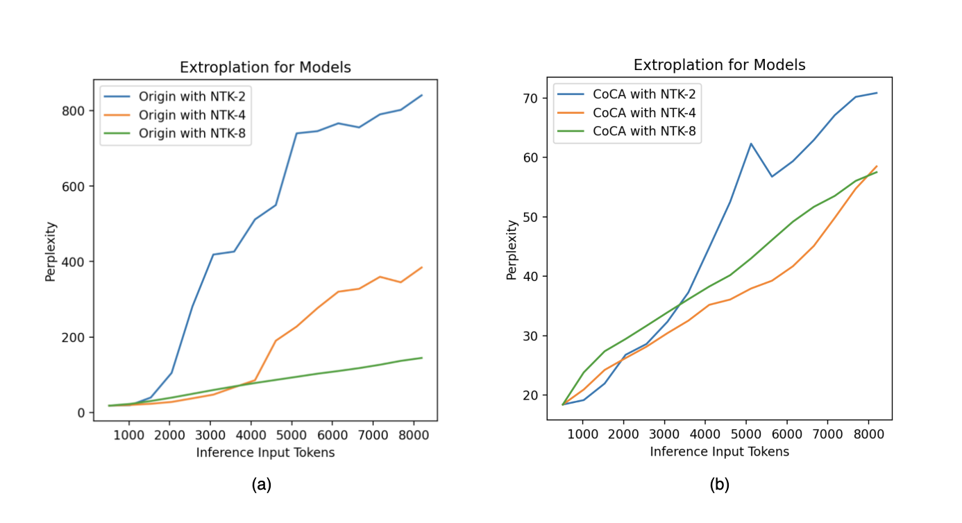
Since we employed the dynamic NTK method for both CoCA and Origin models in inference, we further studied their hyper-parameter stability of scaling factor.

As shown in Figure6, the perplexity of Origin model with different scaling factors undergo drastic changes. In contrast, CoCA performs a stable perplexity for each different choices. Further more, the highest perplexity of CoCA were $50\%+$ lower than the best of Origin model with scaling factors of 2, 4, and 8. Details have been displayed in Table4.

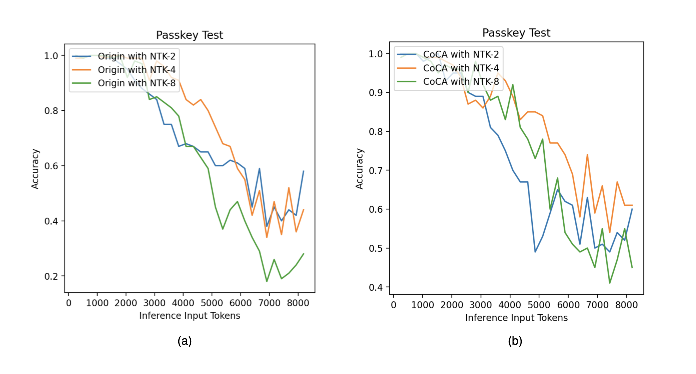
In passkey retrieval, Figure7 shows similar behavior of CoCA and Origin model as that in perplexity measuring. CoCA performs a stable accuracy with different scaling factors and Origin model’s accuracy falls down to $20\%$ or less in the case of scaling factor 8. In Table5, we measured the gap of lowest accuracy between CoCA and Origin model. For the best case of Origin model with scaling factor 2, there still have $5\%-10\%$ gap with CoCA.

Additionally, the perplexity of Origin model in this case of scaling factor 2 performs poorly, it indicates that the Origin model fails to guarantee the performance of language modeling and long-range dependence at the same time.

Figure 6: Perplexity of Origin model and CoCA with different scaling factors. (a) Origin model; (b) CoCA. Perplexity of Origin model varies from 200 to 800, while CoCA varies from 60 to 70.

Table 4: Perplexity with different scaling factors

Model	Sequence length
	512	2048	4096	5632	6656	7680	8192
CoCA(NTK-2)	18.41	26.78	44.84	56.76	62.92	70.18	70.84
CoCA(NTK-4)	18.41	26.23	35.19	39.25	45.10	54.73	58.49
CoCA(NTK-8)	18.41	29.44	38.27	46.11	51.68	56.04	57.51
Origin(NTK-2)	17.96	104.90	511.78	745.80	755.78	802.25	144.48
Origin(NTK-4)	17.96	27.77	85.38	276.57	327.77	345.06	384.34
Origin(NTK-8)	17.96	39.17	78.01	102.71	117.51	136.75	840.95

Figure 7: Passkey accuracy of Origin model and CoCA with different scaling factors. (a) Origin model; (b) CoCA. Accuracy of Origin model varies from $20\%$ to $40\%$, while CoCA varies from $45\%$ to $60\%$.

Table 5: Passkey accuracy with different scaling factors

Model	Sequence length
	512	2048	4096	5632	6656	7680	8192
CoCA(NTK-2)	1.0	0.95	0.7	0.65	0.63	0.54	0.6
CoCA(NTK-4)	1.0	0.97	0.89	0.77	0.74	0.67	0.61
CoCA(NTK-8)	1.0	0.96	0.92	0.68	0.5	0.47	0.45
Origin(NTK-2)	0.99	0.95	0.68	0.62	0.59	0.44	0.58
Origin(NTK-4)	0.99	0.99	0.84	0.67	0.51	0.52	0.44
Origin(NTK-8)	0.99	0.92	0.67	0.44	0.29	0.21	0.28

4.5 Behaviour of attention score in extrapolation

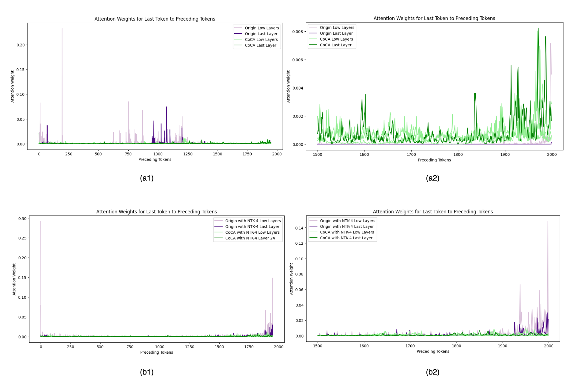
As studied by Chen et al. (2023), extrapolation failure directly related to outliers of attention score. Here we tried to observe this phenomenon through a demonstration. This may explain why CoCA has better extrapolation performance from another aspect.

This demonstration used a random fragment from PG-19 dataset (Rae et al., 2019) with 1,951 tokens, about 4 times of our training length.

Figure 8 demonstrated the attention score of Origin model and CoCA, which indicates as follows:

• From (a1) and (b1), we will find that there are some outliers have extremely large attention score in Origin model, about 10 to 20 times larger than CoCA.

• Because of those outliers that disrupt the observation effect, we enlarged (a1) at last 500 tokens as (a2), attention score of Origin model in last layer almost became 0, it indicates that Origin model failed in attending to neighboring tokens.

• From (b2), after applying dynamic NTK-method, Origin model presents a trend of excessive attention on neighboring tokens. This is highly probable due to severe over-fitting of the nearest tokens during the training phase, as we demonstrated in Section 2.3.

Figure 8: Attention scores in extrapolation, low layers means layer 6, 12, 18, last layer means layer 24. (a1) Attention scores of Origin model and CoCA. (a2) Enlarged version of (a1) at last 500 tokens. (b1) Attention scores of Origin model and CoCA with Dynamic NTK-method. (b2) Enlarged version of (b1) at last 500 tokens.

4.6 Case study

As shown in Table6, we found some interesting cases of CoCA model’s output. It somehow exhibits a unique characteristic like creativeness. Additional comments were made on the question itself by CoCA, while Origin and ALibi model just repeat those sentences mentioned in the prompt. We don’t known why and how does it happen yet and left this for further works.

Table 6: Output cases of CoCA

CoCA result
80854$\backslash$n I have to say that I am not a fan of the pass key. It is not a good pass key. It is not a good pass key. It is not a good pass key. It is not a good pass key. It is not a good pass key. It is not a good pass
91625$\backslash$n I am not sure.$\backslash$n I am not sure.$\backslash$n I am not sure.$\backslash$n I am not sure.$\backslash$n I am not sure.$\backslash$n I am not sure.$\backslash$n I am not sure.$\backslash$n I am not sure.$\backslash$n I am not sure.$\backslash$n I am not sure.$\backslash$n I
66186$\backslash$n I will ask you to memorize the pass key.$\backslash$n The grass is green. The sky is blue. The sun is yellow. Here we go.$\backslash$n What is the pass key?$\backslash$n I will ask you to memorize the pass key.$\backslash$n The grass is green. The sky is

5 Conclusions

In this work, we observed an anomalous behavior between RoPE and attention matrices, which severely leads to a chaos of position embedding, especially at closest positions containing critical information. To address this at its core, we introduced a new self-attention framework called Collinear Constrained Attention (CoCA). We provided mathematical evidence showcasing the superior characteristics of our method, such as a strong form of long-term decay, as well as computational and spatial efficiency for practical applications. Experimental findings confirm that CoCA delivers outstanding performance in both long-sequence language modeling and capturing long-range dependence. Additionally, CoCA seamlessly integrates with existing extrapolation, interpolation techniques, and other optimization methods designed for conventional Transformer models. This adaptability suggests that CoCA has the potential to evolve into an enhanced version of Transformer models.

Appendix A Rotary borders

For simplicity, let’s take the example of Figure 3, there are three borders during rotating. As shown in Figure 9. We use the relative coordinate system by regarding ${\mathbf{q}}_{j}$ as $x$-axis:

• The first border is ${\mathbf{k}}_{j}$.

• The second border is $-{\mathbf{q}}_{j}$.

• The last border is ${\mathbf{q}}_{j}$.

Every time when the relative angle of ${\mathbf{q}}_{j}$ and ${\mathbf{k}}_{j}$ crossover these borders, the monotonicity of $a(m,n)$ will perform a reversal. Leading the model confusing when extrapolating.

CoCA fundamentally solved the problem of the border of ${\mathbf{k}}_{j}$, and we applied dynamic NTK method(no fine-tuning) here both in CoCA and Origin model during inference for passkey retrieval to reduce the confusion of $-{\mathbf{q}}_{j}$ and ${\mathbf{q}}_{j}$.

Apart from applying NTK to reduce the confusion of $-{\mathbf{q}}_{j}$ and ${\mathbf{q}}_{j}$, it might be more effective by limiting the rotary boundary at the beginning of training. We left this for future works.

Figure 9: Relative coordinate system by regarding ${\mathbf{q}}_{j}$ as $x$-axis

Appendix B Parity check retrieval

Experiments are not completed yet.

References

- a. Smith & Gray (2018) Daniel G. a. Smith and Johnnie Gray. opt_einsum - a python package for optimizing contraction order for einsum-like expressions. Journal of Open Source Software, 3(26):753, 2018. doi: 10.21105/joss.00753. URL https://doi.org/10.21105/joss.00753.
- Black et al. (2022) Sidney Black, Stella Biderman, Eric Hallahan, Quentin Anthony, Leo Gao, Laurence Golding, Horace He, Connor Leahy, Kyle McDonell, Jason Phang, Michael Pieler, Usvsn Sai Prashanth, Shivanshu Purohit, Laria Reynolds, Jonathan Tow, Ben Wang, and Samuel Weinbach. GPT-NeoX-20B: An open-source autoregressive language model. In Proceedings of BigScience Episode #5 – Workshop on Challenges & Perspectives in Creating Large Language Models, pp. 95–136, virtual+Dublin, May 2022. Association for Computational Linguistics. doi: 10.18653/v1/2022.bigscience-1.9. URL https://aclanthology.org/2022.bigscience-1.9.
- bloc97 (2023) bloc97. Ntk-aware scaled rope allows llama models to have extended (8k+) context size without any fine-tuning and minimal perplexity degradation, 2023. URL https://www.reddit.com/r/LocalLLaMA/comments/14lz7j5/ntkaware_scaled_rope_allows_llama_modes_to_have/.
- Chen et al. (2023) Shouyuan Chen, Sherman Wong, Liangjian Chen, and Yuandong Tian. Extending context window of large language models via positional interpolation. ArXiv, abs/2306.15595, 2023. URL https://api.semanticscholar.org/CorpusID:259262376.
- Chi et al. (2022) Ta-Chung Chi, Ting-Han Fan, Peter J. Ramadge, and Alexander I. Rudnicky. Kerple: Kernelized relative positional embedding for length extrapolation. ArXiv, abs/2205.09921, 2022. URL https://api.semanticscholar.org/CorpusID:248965309.
- Devlin et al. (2019) Jacob Devlin, Ming-Wei Chang, Kenton Lee, and Kristina Toutanova. Bert: Pre-training of deep bidirectional transformers for language understanding. ArXiv, abs/1810.04805, 2019. URL https://api.semanticscholar.org/CorpusID:52967399.
- Du et al. (2021) Zhengxiao Du, Yujie Qian, Xiao Liu, Ming Ding, Jiezhong Qiu, Zhilin Yang, and Jie Tang. Glm: General language model pretraining with autoregressive blank infilling. In Annual Meeting of the Association for Computational Linguistics, 2021. URL https://api.semanticscholar.org/CorpusID:247519241.
- Foundation (2021) Wikimedia Foundation. Wikimedia downloads, 2021. URL https://dumps.wikimedia.org.
- Gao et al. (2020) Leo Gao, Stella Rose Biderman, Sid Black, Laurence Golding, Travis Hoppe, Charles Foster, Jason Phang, Horace He, Anish Thite, Noa Nabeshima, Shawn Presser, and Connor Leahy. The pile: An 800gb dataset of diverse text for language modeling. ArXiv, abs/2101.00027, 2020. URL https://api.semanticscholar.org/CorpusID:230435736.
- Loshchilov & Hutter (2017) Ilya Loshchilov and Frank Hutter. Fixing weight decay regularization in adam. ArXiv, abs/1711.05101, 2017. URL https://api.semanticscholar.org/CorpusID:3312944.
- Mohtashami & Jaggi (2023) Amirkeivan Mohtashami and Martin Jaggi. Landmark attention: Random-access infinite context length for transformers. ArXiv, abs/2305.16300, 2023. URL https://api.semanticscholar.org/CorpusID:258887482.
- Paszke et al. (2019) Adam Paszke, Sam Gross, Francisco Massa, Adam Lerer, James Bradbury, Gregory Chanan, Trevor Killeen, Zeming Lin, Natalia Gimelshein, Luca Antiga, et al. Pytorch: An imperative style, high-performance deep learning library. Advances in neural information processing systems, 32, 2019.
- Press et al. (2021) Ofir Press, Noah A. Smith, and Mike Lewis. Train short, test long: Attention with linear biases enables input length extrapolation. ArXiv, abs/2108.12409, 2021. URL https://api.semanticscholar.org/CorpusID:237347130.
- Rae et al. (2019) Jack W. Rae, Anna Potapenko, Siddhant M. Jayakumar, and Timothy P. Lillicrap. Compressive transformers for long-range sequence modelling. ArXiv, abs/1911.05507, 2019. URL https://api.semanticscholar.org/CorpusID:207930593.
- Su et al. (2021) Jianlin Su, Yu Lu, Shengfeng Pan, Bo Wen, and Yunfeng Liu. Roformer: Enhanced transformer with rotary position embedding. ArXiv, abs/2104.09864, 2021. URL https://api.semanticscholar.org/CorpusID:233307138.
- Sun et al. (2022) Yutao Sun, Li Dong, Barun Patra, Shuming Ma, Shaohan Huang, Alon Benhaim, Vishrav Chaudhary, Xia Song, and Furu Wei. A length-extrapolatable transformer. ArXiv, abs/2212.10554, 2022. URL https://api.semanticscholar.org/CorpusID:254877252.
- Touvron et al. (2023) Hugo Touvron, Thibaut Lavril, Gautier Izacard, Xavier Martinet, Marie-Anne Lachaux, Timothée Lacroix, Baptiste Rozière, Naman Goyal, Eric Hambro, Faisal Azhar, Aurelien Rodriguez, Armand Joulin, Edouard Grave, and Guillaume Lample. Llama: Open and efficient foundation language models. ArXiv, abs/2302.13971, 2023. URL https://api.semanticscholar.org/CorpusID:257219404.
- Tworkowski et al. (2023) Szymon Tworkowski, Konrad Staniszewski, Mikolaj Pacek, Yuhuai Wu, Henryk Michalewski, and Piotr Milo’s. Focused transformer: Contrastive training for context scaling. ArXiv, abs/2307.03170, 2023. URL https://api.semanticscholar.org/CorpusID:259360592.
- Vaswani et al. (2017) Ashish Vaswani, Noam Shazeer, Niki Parmar, Jakob Uszkoreit, Llion Jones, Aidan N Gomez, Łukasz Kaiser, and Illia Polosukhin. Attention is all you need. Advances in neural information processing systems, 30, 2017.
- Zhao et al. (2023) Yanli Zhao, Andrew Gu, Rohan Varma, Liangchen Luo, Chien chin Huang, Min Xu, Less Wright, Hamid Shojanazeri, Myle Ott, Sam Shleifer, Alban Desmaison, Can Balioglu, Bernard Nguyen, Geeta Chauhan, Yuchen Hao, and Shen Li. Pytorch fsdp: Experiences on scaling fully sharded data parallel. ArXiv, abs/2304.11277, 2023. URL https://api.semanticscholar.org/CorpusID:258297871.
- Zhu et al. (2015) Yukun Zhu, Ryan Kiros, Richard S. Zemel, Ruslan Salakhutdinov, Raquel Urtasun, Antonio Torralba, and Sanja Fidler. Aligning books and movies: Towards story-like visual explanations by watching movies and reading books. 2015 IEEE International Conference on Computer Vision (ICCV), pp. 19–27, 2015. URL https://api.semanticscholar.org/CorpusID:6866988.