NISF: Neural Implicit Segmentation Functions

Abstract

Segmentation of anatomical shapes from medical images has taken an important role in the automation of clinical measurements. While typical deep-learning segmentation approaches are performed on discrete voxels, the underlying objects being analysed exist in a real-valued continuous space. Approaches that rely on convolutional neural networks (CNNs) are limited to grid-like inputs and not easily applicable to sparse or partial measurements. We propose a novel family of image segmentation models that tackle many of CNNs’ shortcomings: Neural Implicit Segmentation Functions (NISF). Our framework takes inspiration from the field of neural implicit functions where a network learns a mapping from a real-valued coordinate-space to a shape representation. NISFs have the ability to segment anatomical shapes in high-dimensional continuous spaces. Training is not limited to voxelized grids, and covers applications with sparse and partial data. Interpolation between observations is learnt naturally in the training procedure and requires no post-processing. Furthermore, NISFs allow the leveraging of learnt shape priors to make predictions for regions outside of the original image plane. We go on to show the framework achieves dice scores of $0.87\pm 0.045$ on a (3D+t) short-axis cardiac segmentation task using the UK Biobank dataset. We also provide a qualitative analysis on our frameworks ability to perform segmentation and image interpolation on unseen regions of an image volume at arbitrary resolutions.

1 Introduction

Image segmentation is a core task in domains where the area, volume or surface of an object is of interest. The principle of segmentation involves assigning a class to every presented point in the input space. Typically, the input is presented in the form of images: aligned pixel (or voxel) grids, with the intention to obtain a class label for each. In this context, the application of deep learning to the medical imaging domain has shown great promise in recent years. With the advent of the U-Net [20], Convolutional Neural Networks (CNN) have been successfully applied to a multitude of imaging domains and achieved (or even surpassed) human performance [11]. The convolution operation make CNNs an obvious choice for dealing with inputs in the form of 2D pixel- or 3D voxel-grids.

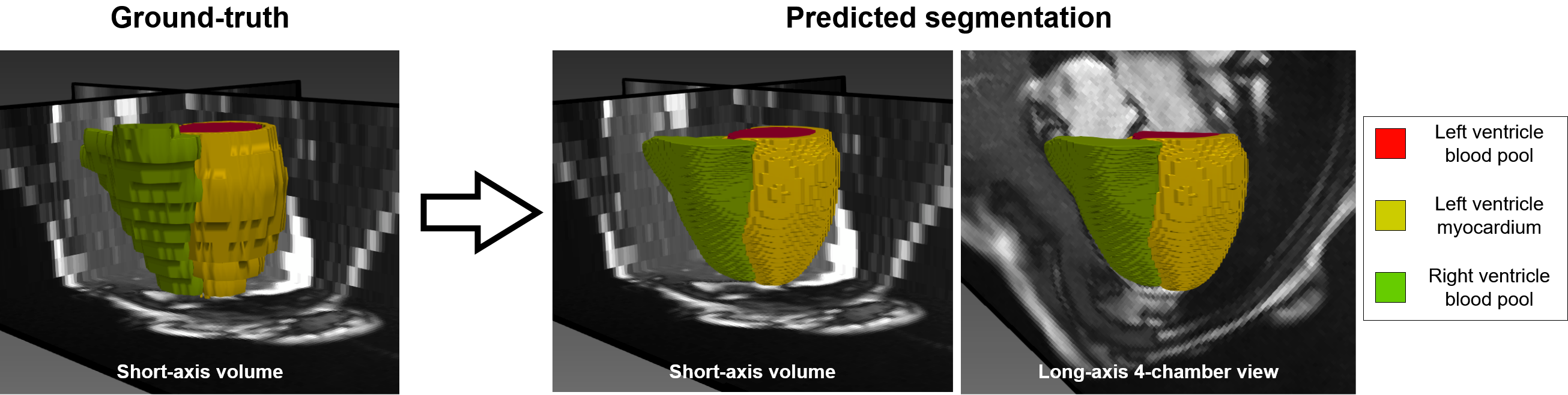
Figure 1: Short axis volumes have low resolution along the ventricle’s long axis. Given a short axis image volume, a NISF can produce arbitrary resolution segmentations along the long axis.

Despite their efficacy, CNNs suffer from a range of limitations that lead to incompatibilities for some imaging domains. CNNs are restricted to data in the form of grids, and cannot easily handle sparse or partial inputs. Moreover, due to the CNN’s segmentation output also being confined to a grid, obtaining smooth object surfaces requires post-processing heuristics. Predicting a high resolution segmentations also has implications on the memory and compute requirements in high-dimensional domains. Finally, the learning of long-distance spatial correlations requires deep stacks of layers, which may pose too taxing in low resource domains.

We introduce a novel approach to image segmentation that circumvents these shortcomings: Neural Implicit Segmentation Functions (NISF). Inspired by ongoing research in the field of neural implicit functions (NIF), a neural network is taught to learn a mapping from a coordinate space to any arbitrary real-valued space, such as segmentation, distance function, or image intensity. While CNNs employ the image’s pixel or voxel intensities as an input, NISF’s input is a real-valued vector $c\in\mathbb{R}^{N}$ for a single N-dimensional coordinate, alongside a subject-specific latent representation vector $h\in\mathbb{R}^{d}$. Given $c$ and $h$, the network is taught to predict image intensity and segmentation value pairs. The space $\mathcal{H}$ over all possible latent vectors $h$ serves as a learnable prior over all possible subject representations.

In this paper, we describe an auto-decoder process by which a previously unseen subject’s pairs of coordinate-image intensity values $(c,i)$ may be used to approximate that subject’s latent representation $h$. Given a latent code, the intensity and segmentation predictions from any arbitrary coordinates in the volume may be sampled. We evaluate the proposed framework’s segmentation scores and investigate its generalization properties on the UK-Biobank cardiac magnetic resonance imaging (MRI) short-axis dataset. We make the source code publicly available.

2 Related Work

Cardiac MRI.  Cardiac magnetic resonance imaging (MRI) is often the preferred imaging modality for the assessment of function and structure of the cardiovascular system. This is in equal parts due to its non-invasive nature, and due to its high spatial and temporal resolution capabilities. The short-axis (SAX) view is a (3+t)-dimensional volume made up of stacked cross-sectional (2D+t) acquisitions which lay orthogonal to the ventricle’s long axis (see Figure 1). Spatial resolution is highest in-plane (typically $<$3mm²), with a much lower inter-slice resolution ( 10mm), and a temporal resolution of $\leq$45ms [15]. On the other hand, long-axis (LAX) views are (2D+t) acquisitions orthogonal to the SAX plane and provide high resolution along the ventricle’s long axis.

Image segmentation.  The capabilities of the CNN has caused it to become the predominant choice for image segmentation tasks [8, 20]. However, a pitfall of these models is their poor generalization to certain input transformations. One such transformation is scaling. This drawback limits the use of CNNs on domains with large variations in pixel spacings. Past works have attempted to mitigate this issue by accounting for dataset characteristics [11], building resilience through augmentations [29], or using multi-scale feature extractors [5].

Additionally, segmentation performed by fully convolutional model is restricted to predicting in pixel (or voxel) grids. This requires post-processing heuristics to extract smooth object surfaces. Works such as [19, 12] try to mitigate this issue through point-wise decoders that operate on interpolated convolutional features. Alternatives to binarized segmentation have been recently proposed such as soft segmentations [7] and distance field predictions [6, 24]. Smoothness can also be improved by predicting at higher resolutions. This is however limited by the exponential increase of memory that comes with high-dimensional data. Partitioning of the input can make memory requirements manageable [3, 9], but doing so disallows the ability to learn long-distance spatial correlations.

Neural implicit functions.  In recent years, NIFs have achieved notable milestones in the field of shape representations [17, 18]. NIFs have multiple advantages over classical voxelized approaches that makes them remarkably interesting for applications in the medical imaging domain [10, 28]. First, NIFs can sample shapes at any points in space at arbitrary resolutions. This makes them particularly fit for working with sparse, partial, or non-uniform data. Implicit functions thus remove the need for traditional interpolation as high-resolution shapes are learnt implicitly by the network [1]. This is specially relevant to the medical imaging community, where scans may have complex sampling strategies, have missing or unusable regions, or have highly anisotropic voxel sizes. These properties may further vary across scanners and acquisition protocols, making generalization across datasets a challenge. Additionally, the ability to process each point independently allows implicit functions to have flexible optimization strategies, making entire volumes be optimizable holistically.

Image priors.  The typical application of a NIF involves the training of a multi-layer perceptron (MLP) on a single scene. Although generalization still occurs in generating novel views of the target scene, the introduction of prior knowledge and conditioning of the MLP is subject to ongoing research [1, 14, 16, 18, 22, 23]. Approaches such as [1, 18] opt for auto-decoder architectures where the network is modulated by latent code at the input level. At inference time, the latent code of the target scene is optimized by backpropagation. Works such as [16] choose to instead modulate the network at its activation functions. Other frameworks obtain the latent code in a single-shot fashion through the use of an encoder network [14, 16, 23, 22]. This latent code is then used by a hyper-network [14, 16, 23] or a meta-learning approach [22] to generate the weights of a decoder network.

3 Methods

Shared Prior.  In order to generalize to unseen subjects, we attempt to build a shared prior $\mathcal{H}$ over all subjects. This is done by conditioning the classifier with a latent vector $h\in\mathbb{R}^{d}$ at the input level. Each individual subject $j$ in a population $X$, can be thought of having a distinct $h_{j}$ that serves as a latent code of their unique features. Following [1, 18], we initialize a matrix $H\in\mathbb{R}^{Xd}$, where each row is a latent vector $h_{j}$ corresponding to a single subject $j$ in the dataset. The latent vector $h_{j}$ of a subject is fed to the MLP alongside a point’s coordinate and can be optimized through back-propagation. This allows $\mathcal{H}$ to be optimized to capture useful inter-patient features.

Model Architecture.  The architecture is composed of a segmentation function $f_{\theta}$ and a reconstruction function $f_{\phi}$. At each continuous-valued coordinate $c~{}\in~{}\mathbb{R}^{N}$, function $f_{\theta}$ models the shape’s segmentation probability $s_{c}$ for all $M$ classes, and function $f_{\phi}$ models the image intensity $i_{c}$. The functions are conditioned by a latent vector $h$ at the input level as follows:

$$f_{\theta}:\left(c\in\mathbb{R}^{N}\right)\times\left(h\in\mathbb{R}^{d}\right)\rightarrow s_{c}\in[0,1]^{M},\quad\sum^{M}_{i=1}s_{c}^{i}=1$$ (1)

$$f_{\phi}:\left(c\in\mathbb{R}^{N}\right)\times\left(h\in\mathbb{R}^{d}\right)\rightarrow i_{c}\in[0,1]$$ (2)

In order to improve local agreement between the segmentation and reconstruction functions, we jointly model $f_{\theta}$ and $f_{\phi}$ by a unique multi-layer perceptron (MLP) with two output heads (Figure 2). We employ Gabor wavelet activation functions [21] which are known to be more expressive than Fourier Features combined with ReLU [26] or sinusoidal activation functions [23].

Prior Training.  Following the setup described in [1], we randomly initialize the matrix $H$ consisting of a trainable latent vector $h_{j}\sim\mathcal{N}\left(0,10^{-2}\right)$ for each subject in the training set. On each training sample, the parameters of the MLP are jointly optimized with the subject’s $h_{j}$. We select a training batch by uniformly sampling a time frame $t$ and using all points within that 3D volume. Each voxel in the sample is processed in parallel along the batch dimension. Coordinates are normalized to the range $[0,1]$ based on the voxel’s relative position.

The difference in image reconstruction from the ground-truth voxel intensities is supervised using binary cross-entropy (BCE). This is motivated by our data’s voxel intensity distribution being heavily skewed towards the extremes. The segmentation loss is a sum of a BCE loss component and a Dice loss component. We found that adding a weighting factor of $\alpha=10$ to the image reconstruction loss component yielded inference-time improvements on both image reconstruction and segmentation metrics. Additionally, L2 regularization is applied to the latent vector $h_{j}$ and the MLP’s parameters. The full loss is summarized as follows:

$$\mathcal{L}_{train}(\theta,\phi,h_{j})\;=\;\mathcal{L}_{BCE}\Big{(}f_{\theta}(c,h_{j}),s_{c}\Big{)}\;+\;\mathcal{L}_{Dice}\Big{(}f_{\theta}(c,h_{j}),s_{c}\Big{)}$$ (3)

$$\qquad\qquad+\;\;\alpha\>\mathcal{L}_{BCE}\Big{(}f_{\phi}(c,h_{j}),i_{c}\Big{)}\;+\;\mathcal{L}_{L2}(\theta)\;+\;\mathcal{L}_{L2}(\phi)\;+\;\mathcal{L}_{L2}(h_{j})$$

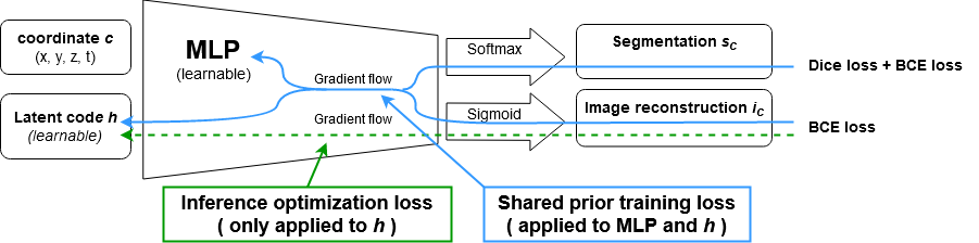
Figure 2: Training and inference setups. During the prior’s training, the MLP and the input latent code $h$ are jointly optimized on image reconstruction and segmentation losses (solid blue line). At inference, solely the latent code $h$ is optimized exclusively on the image reconstruction (dashed green line).

Inference.  Once the segmentation function $f_{\theta}$ has learnt a mapping from the population prior $\mathcal{H}$ to the segmentation space $S$, inference becomes a task of finding a latent code $h$ within $\mathcal{H}$ that correctly models the new subject’s features. The ground-truth segmentation of a new subject is obviously not available at inference, and it is thus not possible to use $f_{\theta}$ to optimize $h$. However, since both functions $f_{\phi}$ (image reconstruction) and $f_{\theta}$ (segmentation) have been jointly trained by consistently using the same latent vector $h$, we make the following assumption: A latent code $h$ optimized for image reconstruction under $f_{\phi}$ will also produce accurate segmentations under $f_{\theta}$. This assumption makes it possible to use the image reconstruction function $f_{\phi}$ alone to find a latent code $h$ for an unseen image in order to generalize segmentation predictions using $f_{\theta}$.

For this task, a new $h\sim\mathcal{N}\left(0,10^{-4}\right)$ is initialized. The weights of the MLP are frozen, such that the only tuneable parameters are those of $h$. Optimization is performed exclusively on the image reconstruction loss (dashed green line in Figure 2):

$$\mathcal{L}_{infer}(h_{j})\;=\;\mathcal{L}_{BCE}\Big{(}f_{\phi}(c,h_{j}),i_{c}\Big{)}\;+\;\mathcal{L}_{L2}(h_{j})$$ (4)

Due to the loss being composed exclusively by the image reconstruction term, $h$ is expected to eventually overfit to $f_{\phi}$. Special care should be taken to find a step-number hyperparameter that stops the optimization of $h$ at the optimal segmentation performance. In our experiments, we chose this parameter based on the Dice score of the best validation run.

4 Experiments and Results

Data overview.  The dataset consists of a random subset of 1150 subjects from the UK Biobank’s short-axis cardiac MRI acquisitions [25]. An overview of the UK Biobank cohort’s baseline statistics can be found in their showcase website [27]. The dataset split included 1000 subjects for the prior training, 50 for validation, and 100 for testing. The (3D+t) short-axis volumes are anisotropic in nature and have a wide range of shapes and pixel spacings along the spatial dimensions. No form of preprocessing was performed on the images except for an intensity normalization to the range $[0,1]$ as performed in similar literature [2]. The high dimensionality of (3D+t) volumes makes manual annotation prohibitively time consuming. Due to this, we make use of synthetic segmentation as ground truth shapes created using a trained state of the art segmentation CNN provided by [2]. The object of interest in each scan is composed of three distinct, mutually exclusive sub-regions: The left ventricle (LV) blood pool, LV myocardium, and right ventricle (RV) blood pool (see Figure 1).

Implementation details.  The architecture consists of 8 residual layers, each with 128 hidden units. The subject latent codes had 128 learnable parameters. The model was implemented using Pytorch and trained on an NVIDIA A40 GPU for 1000 epochs, lasting approximately 9 days. Inference optimization lasted 3-7 minutes per subject depending on volume dimensions. Losses are minimized using the ADAM optimizer [13] using a learning rate of $10^{-4}$ during the prior training training and $10^{-4}$ during inference.

Results.  As the latent code is optimized during inference, segmentation metrics follow an overfitting pattern (see Figure 3). This is an expected consequence of the inference process optimizing solely on the image reconstruction loss. Early stopping should be employed to obtain the best performing latent code state.

The benefits of training a prior over the population is investigated by tracking inference-time Dice scores obtained from spaced-out validation runs. Training of the prior is shown to significantly improve performance of segmentation and image reconstruction at inference-time as seen in Figure 4.

Table 1: Class Dice scores for the 100 subject test dataset.

Class	Classes average	LV blood Pool	LV myocardium	RV blood Pool
Dice score	$0.87\pm 0.045$	$0.90\pm 0.037$	$0.82\pm 0.075$	$0.88\pm 0.063$

Validation results showed the average optimal number of latent code optmimization steps at inference to be 672. Thus, the test set per-class Dice scores (Table 1) were obtained after 672 optimization steps on $h$ for each test subject.

Further investigation is performed on the generalization capabilities of the subject prior by producing segmentations for held-out sections of the image volume. First, the subject’s latent code is optimized using the inference process. Then, the model’s output is sampled at the held-out region’s coordinates.

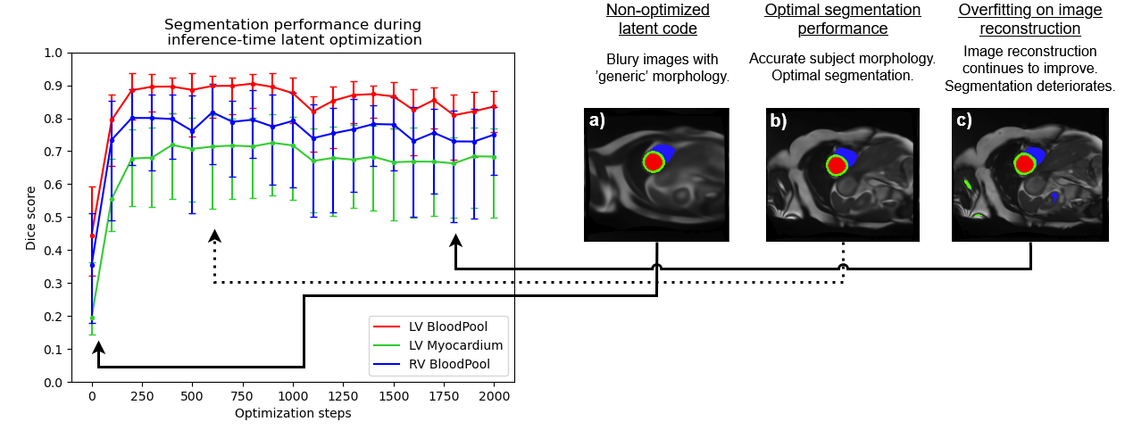
Figure 3: Segmentation Dice trend during a subject’s inference. Early stopping is important to prevent overfitting on reconstruction task. a) Non-optimized latent code creates blurry images with ’generic’ morphology. b) As the latent code is optimized, subject morphology begins to be accurately reconstructed. Segmentation performance reaches an optimum. c) Reconstruction continues to improve, but segmentation deteriorates.

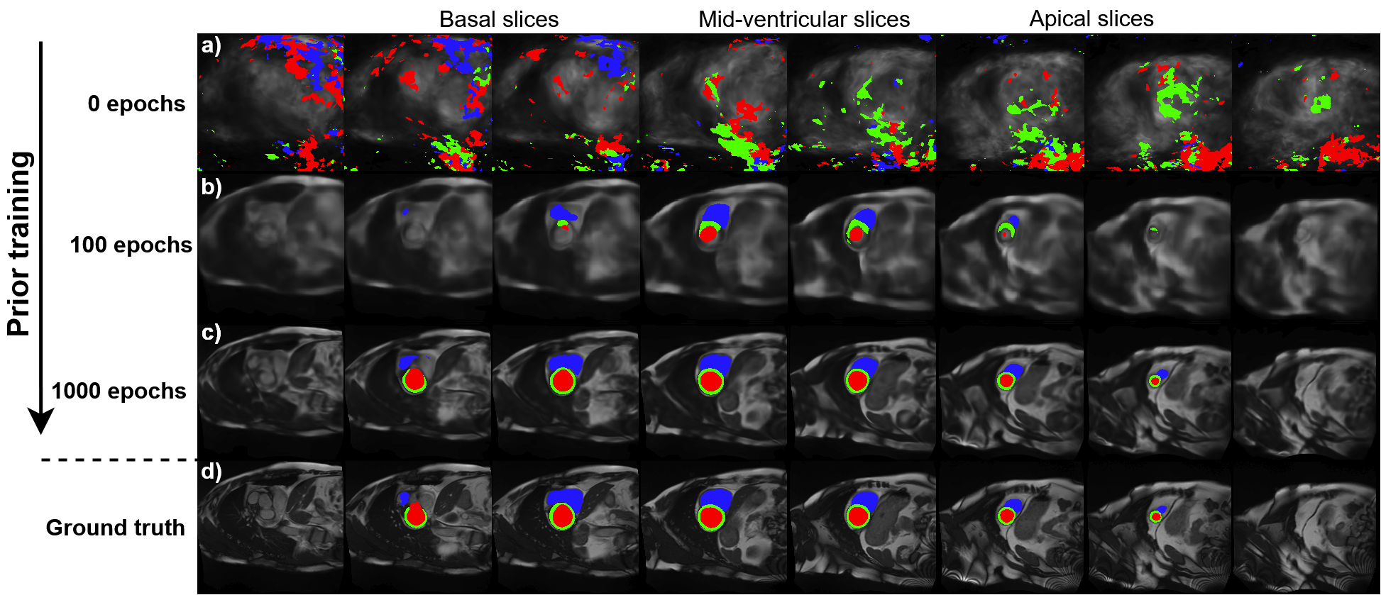
Figure 4: Inference-time segmentation and image reconstruction at various stages of the prior’s training process. a) Prior has not been trained. Inference can roughly reconstruct the image outline. Segmentation fails. b) Early on, reconstructed images are blurry. Segmentation is poor, but at the correct region. c) Eventually images are reconstructed with great detail and segmentations are accurate. d) Ground truth.

Right ventricle segmentation in basal slices is notoriously challenging to manually annotate due to the delineation of the atrial and ventricular cavity combined with the sparsity of the resolution along the long axis [4]. Nonetheless, as seen in Figure 5, our approach is capable of capturing smooth and plausible morphology of these regions despite not having access to the image information.

We go on to show NISF’s ability to generate high-resolution segmentation for out-of-plane views. We optimize on a short-axis volume at inference and subsequently sample coordinates corresponding to long-axis views. Despite never presenting a ground-truth long-axis image, the model reconstructs an interpolated view and provides an accurate segmentation along its plane (Figure 6).

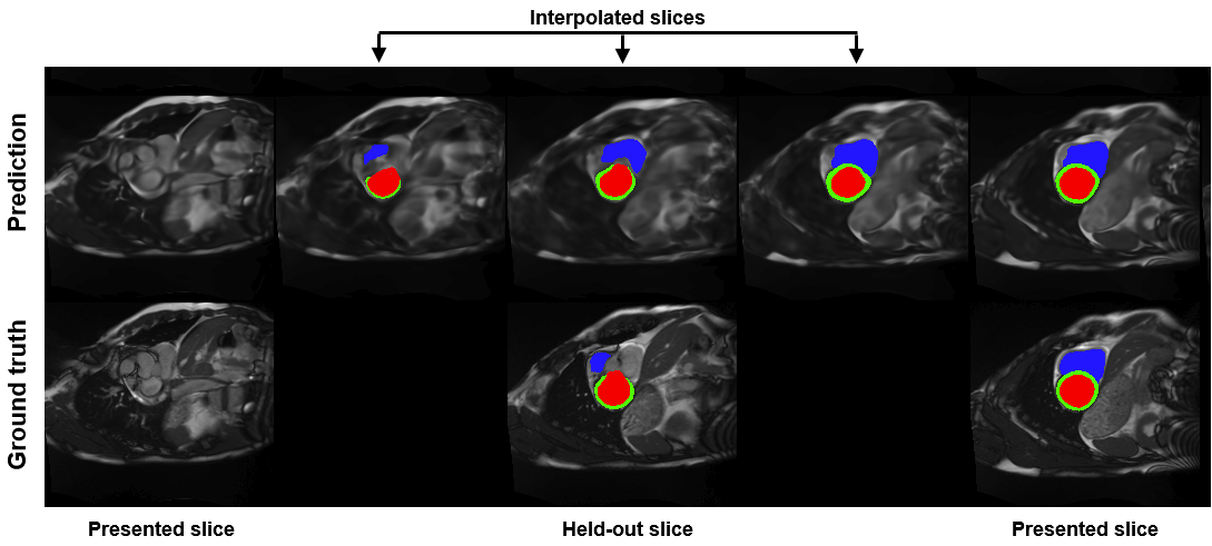
Figure 5: Interpolation predictions for a held-out basal slice. Top row: Predicted segmentation overlayed on predicted image. Bottom row: Ground truth segmentation overlayed on original image. Middle column is never shown to network during inference. Black slices don’t exist in original image volume. The model appears to understand how the ventricles come into view as we descend down the slice dimension.

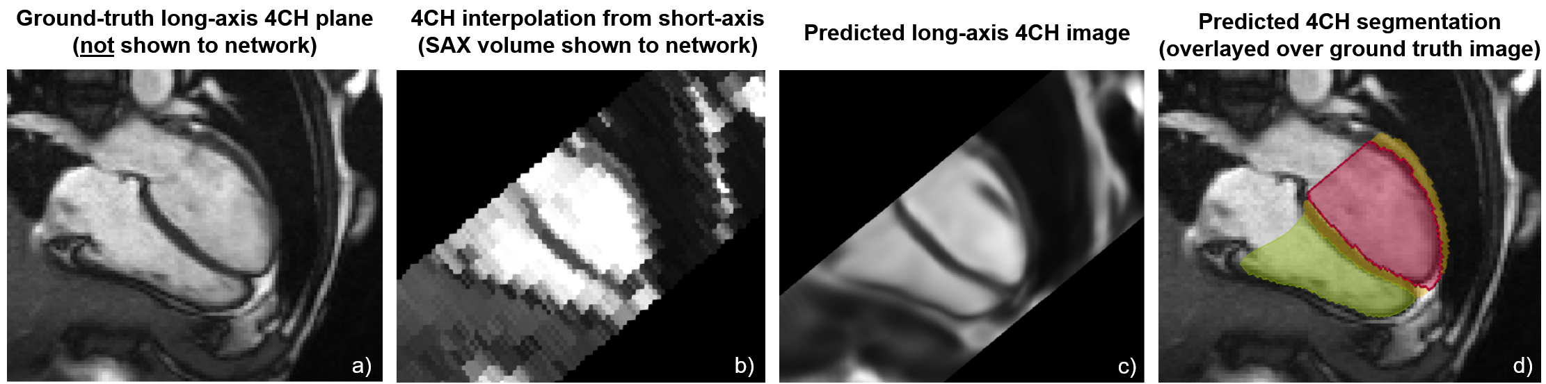
Figure 6: Segmentation of a held-out long-axis 4-chamber plane from SAX image data. a) Ground-truth long-axis 4-chamber view (not presented to network). b) Nearest-neighbour interpolation of 4-chamber view from SAX volume. c) Predicted 4-chamber image plane. d) Predicted 4-chamber view segmentation.

5 Conclusion

We present a novel family of image segmentation models that can model shapes at arbitrary resolutions. The approach is able to leverage priors to make predictions for regions not present in the original image data. Working directly on the coordinate space has the benefit of accepting high-dimensional sparse data, as well as not being affected by variations in image shapes and resolutions. We implement a simple version of this framework and evaluate it on a short-axis cardiac MRI segmentation task using the UK Biobank. Reported Dice scores on 100 unseen subjects average $0.87\pm 0.045$. We also perform a qualitative analysis on the framework’s ability to predict held-out sections of image volumes.

6 Acknowledgements

This work is funded by the Munich Center for Machine Learning and European Research Council (ERC) project Deep4MI (884622). This research has been conducted using the UK Biobank Resource under Application Number 87802.

References

- [1] Amiranashvili, T., Lüdke, D., Li, H.B., Menze, B., Zachow, S.: Learning shape reconstruction from sparse measurements with neural implicit functions. In: International Conference on Medical Imaging with Deep Learning. pp. 22–34. PMLR (2022)
- [2] Bai, W., Sinclair, M., Tarroni, G., Oktay, O., Rajchl, M., Vaillant, G., Lee, A.M., Aung, N., Lukaschuk, E., Sanghvi, M.M., et al.: Automated cardiovascular magnetic resonance image analysis with fully convolutional networks. Journal of Cardiovascular Magnetic Resonance 20(1), 1–12 (2018)
- [3] Bali, A., Singh, S.N.: A review on the strategies and techniques of image segmentation. In: 2015 Fifth International Conference on Advanced Computing & Communication Technologies. pp. 113–120. IEEE (2015)
- [4] Budai, A., Suhai, F.I., Csorba, K., Toth, A., Szabo, L., Vago, H., Merkely, B.: Fully automatic segmentation of right and left ventricle on short-axis cardiac MRI images. Computerized Medical Imaging and Graphics 85, 101786 (2020)
- [5] Chen, L.C., Yang, Y., Wang, J., Xu, W., Yuille, A.L.: Attention to scale: Scale-aware semantic image segmentation. In: Proceedings of the IEEE conference on computer vision and pattern recognition. pp. 3640–3649 (2016)
- [6] Dai, A., Ruizhongtai Qi, C., Nießner, M.: Shape completion using 3D-encoder-predictor CNNs and shape synthesis. In: Proceedings of the IEEE conference on computer vision and pattern recognition. pp. 5868–5877 (2017)
- [7] Gros, C., Lemay, A., Cohen-Adad, J.: SoftSeg: Advantages of soft versus binary training for image segmentation. Medical image analysis 71, 102038 (2021)
- [8] He, K., Zhang, X., Ren, S., Sun, J.: Deep residual learning for image recognition. In: Proceedings of the IEEE conference on computer vision and pattern recognition. pp. 770–778 (2016)
- [9] Hou, L., Samaras, D., Kurc, T.M., Gao, Y., Davis, J.E., Saltz, J.H.: Efficient multiple instance convolutional neural networks for gigapixel resolution image classification. arXiv preprint arXiv:1504.07947 7, 174–182 (2015)
- [10] Huang, W., Li, H., Cruz, G., Pan, J., Rueckert, D., Hammernik, K.: Neural implicit k-space for binning-free non-cartesian cardiac MR imaging. arXiv preprint arXiv:2212.08479 (2022)
- [11] Isensee, F., Jaeger, P.F., Kohl, S.A., Petersen, J., Maier-Hein, K.H.: nnU-Net: a self-configuring method for deep learning-based biomedical image segmentation. Nature methods 18(2), 203–211 (2021)
- [12] Khan, M.O., Fang, Y.: Implicit neural representations for medical imaging segmentation. In: International Conference on Medical Image Computing and Computer-Assisted Intervention. pp. 433–443. Springer (2022)
- [13] Kingma, D.P., Ba, J.: Adam: A method for stochastic optimization. In: 3rd International Conference on Learning Representations, ICLR 2015, San Diego, CA, USA, May 7-9, 2015, Conference Track Proceedings (2015)
- [14] Klocek, S., Maziarka, Ł., Wołczyk, M., Tabor, J., Nowak, J., Śmieja, M.: Hypernetwork functional image representation. In: Artificial Neural Networks and Machine Learning–ICANN 2019: Workshop and Special Sessions: 28th International Conference on Artificial Neural Networks, Munich, Germany, September 17–19, 2019, Proceedings 28. pp. 496–510. Springer (2019)
- [15] Kramer, C.M., Barkhausen, J., Bucciarelli-Ducci, C., Flamm, S.D., Kim, R.J., Nagel, E.: Standardized cardiovascular magnetic resonance imaging (CMR) protocols: 2020 update. Journal of Cardiovascular Magnetic Resonance 22(1), 1–18 (2020)
- [16] Mehta, I., Gharbi, M., Barnes, C., Shechtman, E., Ramamoorthi, R., Chandraker, M.: Modulated periodic activations for generalizable local functional representations. In: Proceedings of the IEEE/CVF International Conference on Computer Vision. pp. 14214–14223 (2021)
- [17] Mildenhall, B., Srinivasan, P.P., Tancik, M., Barron, J.T., Ramamoorthi, R., Ng, R.: NeRF: Representing scenes as neural radiance fields for view synthesis. Communications of the ACM 65(1), 99–106 (2021)
- [18] Park, J.J., Florence, P., Straub, J., Newcombe, R., Lovegrove, S.: DeepSDF: Learning continuous signed distance functions for shape representation pp. 165–174 (2019)
- [19] Peng, S., Niemeyer, M., Mescheder, L., Pollefeys, M., Geiger, A.: Convolutional occupancy networks. In: Computer Vision – ECCV 2020. Lecture Notes in Computer Science, 12348, vol. 3, pp. 523–540. Springer (2020)
- [20] Ronneberger, O., Fischer, P., Brox, T.: U-net: Convolutional networks for biomedical image segmentation. In: Medical Image Computing and Computer-Assisted Intervention–MICCAI 2015: 18th International Conference, Munich, Germany, October 5-9, 2015, Proceedings, Part III 18. pp. 234–241. Springer (2015)
- [21] Saragadam, V., LeJeune, D., Tan, J., Balakrishnan, G., Veeraraghavan, A., Baraniuk, R.G.: WIRE: Wavelet Implicit Neural Representations. arXiv preprint arXiv:2301.05187 (2023)
- [22] Sitzmann, V., Chan, E., Tucker, R., Snavely, N., Wetzstein, G.: MetaSDF: Meta-learning signed distance functions. Advances in Neural Information Processing Systems 33, 10136–10147 (2020)
- [23] Sitzmann, V., Martel, J., Bergman, A., Lindell, D., Wetzstein, G.: Implicit neural representations with periodic activation functions. Advances in Neural Information Processing Systems 33, 7462–7473 (2020)
- [24] Stutz, D., Geiger, A.: Learning 3D shape completion from laser scan data with weak supervision. In: Proceedings of the IEEE Conference on Computer Vision and Pattern Recognition. pp. 1955–1964 (2018)
- [25] Sudlow, C., Gallacher, J., Allen, N., Beral, V., Burton, P., Danesh, J., Downey, P., Elliott, P., Green, J., Landray, M., Liu, B., Matthews, P., Ong, G., Pell, J., Silman, A., Young, A., Sprosen, T., Peakman, T., Collins, R.: UK Biobank: An open access resource for identifying the causes of a wide range of complex diseases of middle and old age. PLoS Med 12(3) (2015)
- [26] Tancik, M., Srinivasan, P., Mildenhall, B., Fridovich-Keil, S., Raghavan, N., Singhal, U., Ramamoorthi, R., Barron, J., Ng, R.: Fourier features let networks learn high frequency functions in low dimensional domains. Advances in Neural Information Processing Systems 33, 7537–7547 (2020)
- [27] UK Biobank: Data showcase. https://biobank.ndph.ox.ac.uk/showcase/, accessed: 07 Mar 2023
- [28] Wolterink, J.M., Zwienenberg, J.C., Brune, C.: Implicit neural representations for deformable image registration. In: International Conference on Medical Imaging with Deep Learning. pp. 1349–1359. PMLR (2022)
- [29] Zhao, A., Balakrishnan, G., Durand, F., Guttag, J.V., Dalca, A.V.: Data augmentation using learned transformations for one-shot medical image segmentation. In: Proceedings of the IEEE/CVF conference on computer vision and pattern recognition. pp. 8543–8553 (2019)