Fractal Compressive Sensing

Abstract

This paper introduces a sparse projection matrix composed of discrete (digital) periodic lines that create a pseudo-random fractal (p.frac) sampling scheme. Our approach enables random Cartesian sampling whilst employing deterministic and one-dimensional (1D) trajectories derived from the discrete Radon transform (DRT). Unlike radial trajectories, DRT projections can be back-projected without interpolation. Thus, we also propose a novel reconstruction method based on the exact projections of the DRT called finite Fourier reconstruction (FFR). We term this combined p.frac and FFR strategy, fractal compressive sensing (FCS), with image recovery demonstrated on experimental and simulated data; image quality comparisons are made with Cartesian random sampling in 1D and two-dimensional (2D), as well as radial under-sampling in a more constrained experiment. Our experiments indicate FCS enables 3-5dB gain in peak signal-to-noise ratio (PSNR) for 2-, 4- and 8-fold under-sampling compared to 1D Cartesian random sampling. This paper aims to:

1. Review common sampling strategies for compressed sensing (CS)- magnetic resonance imaging (MRI) to inform the motivation of a projective and Cartesian sampling scheme.

2. Compare the incoherence of these sampling strategies and the proposed p.frac.

3. Compare reconstruction quality of the sampling schemes under various reconstruction strategies to determine the suitability of p.frac for CS-MRI.

It is hypothesised that because p.frac is a highly incoherent sampling scheme, that reconstructions will be of high quality compared to 1D Cartesian phase-encode under-sampling.

I Introduction

The theory of CS [1, 2] is integral to sparse image reconstruction and has seen application in many areas of signal processing [3]. This is especially true for medical applications, where scan times are significantly influenced by available sampling and reconstruction methods [4, 5]. From a signal processing perspective, CS performs optimally when three conditions are met: incoherent under-sampling, transform sparsity and non-linear optimisation. Imaging problems will have unique considerations in these regards, with each involving some compromise to the reconstruction pipeline.

Figure 1: Comparison of 2-fold under-sampling masks: (top) proposed pattern composed of a pseudo-random fractal based on a subset of discrete periodic lines; (bottom) uniform random Cartesian sampling.

To optimally leverage CS we wish to employ an incoherent under-sampling strategy that conserves as much energy of a system as possible, a task synonymous with orthogonal measurement, conforming to the well-known Restricted Isometry Property (RIP), and the preservation of our signal’s $\ell_{2}$-norm [6, 1, 7, 2, 8, 3, 9]. Ideal measurement is therefore non-deterministic or an approximation thereof, as random sampling has been shown to produce incoherence with high probability. It follows that incoherence is directly tied to the distribution of a sampling matrix and provides a measure for its suitability in CS applications. Unfortunately, many fields of signal processing are fundamentally limited by measurement hardware, where random sampling is impractical or impossible to implement. Such constraints often result in reduced incoherence and sub-optimal CS reconstructions. To address this issue, Yu et al. [10] developed a hardware-friendly measurement operator by populating sensing matrices with chaotic sequences, producing an approximately orthogonal sampling matrix via deterministic chaos. Alternatively, Linh-Trung et al. [11] pre-process incoming data with a chaotic filter to reduce coherence between measurements. Theirs and subsequent works have demonstrated reconstruction performance comparable to or greater than purely random equivalents [12, 13, 14, 15, 16, 17, 18, 19].

In this work, we propose an incoherent Fourier sampling pattern termed p.frac as shown in Figure 1, which is composed of pseudo-random lines that are discrete and deterministic in nature. This p.frac maps not only to an approximately orthogonal projective matrix for CS, but shares similar incoherence properties when compared to a uniform 2D random Cartesian pattern. A novel reconstruction algorithm is also developed that maps to the sampling scheme directly. The sampling and reconstruction strategy is termed FCS, its main contributions can be summarised as follows:

1. FCS solves a longstanding problem in CS of providing an orthogonal Fourier projection operator capable of 2D incoherence without interpolation, designed for rapid and deterministic 1D acquisition.

2. Resulting image artefacts are suppressible by traditional CS algorithms with reconstruction performance approaching that of pure Cartesian 2D random patterns.

3. Measurements of the proposed p.frac map to discrete projections that form a periodic sinogram, facilitating efficient reconstruction by means of our FFR algorithm using only the discrete Fourier transform (DFT) and image denoising algorithms.

Figure 2: Flow chart of 8-fold pseudo-random fractal under-sampling: top path applies mask in DRT space; bottom path applies mask in DFT space. Like colours in the mask images indicate the same projection/slice.

We numerically evaluate the incoherence of p.frac compared to Cartesian 1D and 2D sampling patterns via the sidelobe-to-peak ratio (SPR) of their point spread function (PSF), where lower values of SPR correspond with greater incoherence. We also apply the proposed FCS to complex-valued experimental and simulated MRI data and compare the results to other sparse imaging and image recovery methods. MRI provides excellent test conditions for FCS, as traditionally, acquisition is performed along trajectories of $k$-space (discrete Fourier domain). These are dictated by magnetic gradients within a magnetic field, where an acquisition sequence refers to the manner in which gradients are leveraged to collect data. Our proposal is to define these trajectories by the projected lines that construct the p.frac detailed in Section II-B. The intention is to establish the suitability of FCS compared to Cartesian 1D and 2D random acquisition in a practical setting.

Under-sampling in MRI can be modelled by masking $k$-space with fewer trajectories than required for full resolution. In image space, this equates to the convolution of a sampling mask’s PSF and the target image. Cartesian 2D random sampling is therefore characterised by suppressible noise-like image artefacts (ghosts) that arise when random points from $k$-space are selected, described as being optimally compatible with CS-MRI [20]. However, the necessary rapid switching of gradients is impractical to implement as a 2D acquisition sequence [21, 22]. While it is possible to collect 2D data with a three-dimensional (3D) random sequence, the approach is only suitable for volumetric imaging.

Practical Cartesian-based sampling restricts randomness to one dimension of $k$-space, where trajectories along parallel lines are randomly selected and fully sampled [20, 23]. Incoherence is significantly reduced and image artefacts are structured as a consequence, which increases the difficulty of image recovery. Strategies have been developed to mitigate the impact this poses on image quality, a key example being to vary the density of measurement [23, 24, 25, 26], thus ensuring that high energy regions of $k$-space are well captured compared to low energy regions. Alternate approaches include pseudo 2D random under-sampling [27, 28], or proposing to reconstruct an image from 1D columns of $k$-space [29], fully exploiting randomness in the available direction. For these methods however, incoherence is still fundamentally limited to one dimension, facilitating approximations of an optimal sampling strategy.

Radial and spiral trajectories are seemingly favourable under these circumstances, expressing inherent 2D incoherence due to their orthogonal nature [30, 31, 20, 32, 33]. They are also known to be tolerant to motion and their artefacts, becoming sequences of choice for dynamic MRI where temporal resolution is critical [34, 35, 36, 32, 33]. Unfortunately, non-Cartesian sampling lacks an explicit inverse, necessitating interpolation via filtered back projection (image domain) or $k$-space regridding to recover an image [37, 38, 33]. Under-sampling can further lead to unwanted interpolation artefacts, as ambiguity is added to the infinite projective space [39]. Yang et al. therefore proposed use of pseudo-polar trajectories for CS-MRI [40]. Their method required only 1D interpolation via the fractional Fourier transform, expressing the image within a finite projective space. Compared to 2D Cartesian sampling however, it requires $2N$ projections with $2N$ points for an $N\times N$ image and to perform interpolation for every iteration of CS [40, 41].

Image sparsity is another aspect of CS where MRI poses difficulties, as natural images (including MRI) have not been found to be exactly sparse in any pre-defined transform domain [42]. Lustig et al. [20] initially utilised the wavelet transform for sparse image representation, where under-sampling artefacts remain noise-like and images can be recovered. The approach proved useful, but its non-adaptive nature was later shown to be sub-optimal at high reduction factors [43]. This resulted in the active development of adaptive non-local [44, 45], transform-based [46, 47] and dictionary-based sparsity encoders [43, 48]. However, general downsides to sparse encoding include the introduction of additional image transformations, assumptions of image appearance, and necessitating increased calculations per iteration of CS [49]; learned sparse encoders exacerbate additive computation cost. The necessary non-linear reconstruction such as convex optimisation or basis pursuit algorithms are also computationally expensive relative to the fast Fourier transform (FFT). Linear optimisation methods are available for MRI, however current algorithms often require multi-channel data for acceptable image quality [50, 51, 52, 53], and are not seen as an effective stand-alone solution to sparse reconstruction.

Chandra et al. [17] recently demonstrated a novel, structurally chaotic sparse sampling strategy called Chaotic Sensing (ChaoS) that generates turbulent image artefacts from deterministic (i.e. non-random) fractal sampling patterns in $k$-space. The patterns are termed fractal due to the increasingly self-similar structures created when selecting appropriate lines from the DRT. The DRT is composed of discrete, approximately orthogonal projections that form an exact partition of $k$-space [54]. Chandra et al. [17] use these projections for error correction to ensure convergence, recovering MRI images from up to 4-8 times less imaging data with novel finite maximum likelihood expectation maximisation ($\mathpzc{f}$MLEM) and finite simultaneous iterative reconstruction technique ($\mathpzc{f}$SIRT). Their approach to is similar to [55, 42, 56, 57] where high performance natural image denoisers were employed between iteration steps. The key difference between under-sampled radial and DRT projections being that ChaoS maps to a finite projective space, which allows for simple and robust iterative algorithms to be employed between denoising steps.

What remains to be seen in projection-based Fourier CS and CS-MRI in particular, is a suitably incoherent under-sampling method that does not introduce additive computational complexity via interpolation. Ou et al. [58] demonstrated that taking random DRT projections of pre-randomized image data can yield CS reconstructions of higher quality than other orthogonal bases (such as the DFT). Naturally, one questions whether it is possible to design a randomised fractal that can leverage the ChaoS framework into CS and create a 2D incoherent under-sampling operator. Here we present our p.frac, developed to facilitate discrete and projected sparse image reconstruction directly from the discrete Fourier domain without additional transformations (see Figure 2). Further, considering the achievements of recent CS algorithms, its incoherent nature ensures compatibility with existing incoherent solvers. Compared to non-Cartesian acquisition schemes, p.frac avoids the computational overhead and additive reconstruction artefacts associated with interpolation, as well-as requiring just $N+1$ projections for full coverage of $k$-space. Therefore, it is better suited to complex optimisation algorithms as well as image denoising approaches (such as our FFR).

In this paper, p.frac refers to the pseudo-random fractal pattern, FFR the proposed reconstruction method, and FCS the joint p.frac sampling with FFR. Content is organised as follows: Section II introduces relevant theory, such as CS, the DRT as well-as our proposed FCS. We also include details regarding the experiments conducted in this study. Section III provides comparisons between FCS and other acquisition and reconstruction models for MRI. Section IV is the Discussion.

II Methods

II-A Compressed Sensing

One can model CS for MRI by considering an image $\mathbf{x}\in\mathbb{C}^{N}$ and associated $k$-space measurements $\mathbf{y}\in\mathbb{C}^{M}$, such that $\mathbf{y}=F_{\Omega}\mathbf{x}+\mathbf{v}$. Here $F_{\Omega}\in\mathbb{C}^{M\times N}$ represents an under-sampled DFT and $\mathbf{v}$ to be complex Gaussian noise. Eq. $\mathbf{x}=F_{\Omega}^{H}\left[\mathbf{y}-\mathbf{v}\right]$ is ill-posed when $M<N$, but $\mathbf{x}$ can be recovered according to,

$$\operatornamewithlimits{argmin}_{\mathbf{x}}\;||\mathbf{y}-F_{\Omega}\mathbf{x}||_{2}^{2}+\lambda||\Psi\mathbf{x}||_{1},$$ (1)

where $\Psi$ regularises the solution through sparse transformation and $\lambda$ enforces data consistency with $\mathbf{y}$. As incoherence of sampling matrix $F_{\Omega}$ is important for successful implementation of CS [20, 23], the under-sampling operator must be developed to satisfy the requirement. As such, we measure the incoherence of $F_{\Omega}$ via its SPR. SPR can be evaluated as follows: letting $\mathbf{e}_{i}$ be a basis vector with “$1$” at the $i$th location and “$0$” elsewhere, the PSF is,

$$\text{PSF}(i,j)=\mathbf{e}^{*}_{j}F^{H}_{\Omega}F_{\Omega}\mathbf{e}_{i}$$ (2)

and,

$$\text{SPR}=\operatornamewithlimits{max}_{i\neq j}\left|\text{PSF}(i,j)/\text{PSF}(i,i)\right|$$ (3)

Lower SPR corresponds to greater incoherence. While this is not a comprehensive metric, it provides evidence for the suitability of CS with acquisition patterns. We employ the well known wavelet algorithm with total variation minimisation (CS-WV) as proposed by Lustig et al. [20] to compare relative CS performance between various sampling schemes.

II-B Discrete Radon Transform

The DRT is an exact and approximately orthogonal projective transform, composed of discrete (digital) lines within a finite geometry [54, 59]. For an image size $N\times N$ where $N=p^{n}$ and $p$ is prime, these lines can be defined as follows (non-prime sizes are also supported),

$$y \equiv mx+t\;\;\;(mod\;N),$$ (4)

$$x \equiv psy+t\;\;\;(mod\;N).$$ (5)

Here, $m$ and $s$ are discrete slopes,

$$\mathbf{m} =\{m:m<N,\;m\in\mathbb{Z}^{0+}\},$$ (6)

$$\mathbf{s} =\{s:s<N/p,\;s\in\mathbb{N}^{0+}\},$$ (7)

and translates $t$,

$$\mathbf{t} =\{t:t<N,\;t\in\mathbb{N}_{0}\}.$$ (8)

Projection onto discrete Radon space is then given by the following equations,

$$R(m,t) =\sum_{x=0}^{N-1}I(x,\langle mx+t\rangle_{N}),$$ (9)

$$R^{\perp}(s,t) =\sum_{y=0}^{N-1}I(y,\langle psy+t\rangle_{N}),$$ (10)

where $R$ and $R^{\perp}$ contain horizontal and vertical projection translates respectively. In the simplest case where $N$ is prime and $n=1$, $R$ contains $N$ projections and $R^{\perp}$ one, seeing just $N+1$ projections for full coverage of an image. Matúš and Flusser [54] proved that DRT projections correspond to discrete slices of $k$-space in a phenomena known as the discrete Fourier slice theorem ($d$FST). The correlation is similar to Radon projections mapping to the Fourier domain by the Fourier slice theorem (FST) [60]. Therefore a fast inverse of the DRT can be executed as follows:

Figure 3: $k$-space slices for the prime case $N=5$. Colours represent different slopes, zero-frequency coefficient is centred (black). Set of $N+1$ slices tile all of space exactly once.

1. Compute the 1D FFT of DRT projections, resulting in $k$-space slices.

2. Place each slice for $m$ and $s$ in 2D $k$-space at lines corresponding to Eqs. 4 and 5 respectively, with $t=0$.

3. For any point in $k$-space that is sampled more than once, divide their value by the number of contributions made.

4. Invert with the 2D inverse FFT to resolve the image.

Figure 2 demonstrates the equivalence of removing projections of the DRT and the masking of $k$-space in a fractal pattern. Figure 3 illustrates how each slice is drawn onto $k$-space for $N=5$, note that the origin (DC) is sampled in each instance, similarly to Radon slices.

Figure 4: Construction of an $N=257$ pseudo-random fractal with $\mu=16$ deterministic and $48$ random DRT lines (total $64$). From left to right adding the: first $8$ deterministic lines, final $8$ deterministic lines, first $16$ random lines, second $16$ random lines. Finally displaying all $64$ lines.

II-C Pseudo-Random Fractal

As central $k$-space comprises a large portion of natural images, the fractal from ChaoS was designed in part to tile the central region. As such, Chandra et al. [17] discuss the correlation between possible discrete gradients ($m$ or $s$) for an $N\times N$ image, and points tiled by each slice. In this correlation, central $k$-space can be tiled by selecting DRT gradients whose corresponding Farey vector [61] lies closest to the origin [62]. In order to fuse ChaoS and CS, we develop a method to achieve randomness within this structure by initially selecting $\mu$ values of $m$ and $s$ that best tile this region as-per their Farey vector’s distance from the origin. We then select $\nu=\left\lfloor{rN}\right\rfloor-\mu$ lines from pseudo-random values of $(m,s)$, where $r\in[0,1]$ controls the reduction factor. In total, this gives $\left\lfloor{rN}\right\rfloor$ lines each with $N$ points. Figure 1 shows an example of this new p.frac sampling pattern compared to a uniform 2D random Cartesian pattern. We observe “randomness” is generated per-quadrant of $k$-space, as sampling is mirrored and reflected within the DFT. Figure 4 illustrates 5 stages of adding DRT lines for a $257\times 257$ image, the figure demonstrates how central $k$-space is captured by the first $\mu$ deterministic lines (stages $1$ and $2$), with remaining $k$-space tiled by $\nu$ randomised lines.

As far as we are aware, no other Fourier-based sampling pattern can produce such randomness while adhering to deterministic lines or digital projections. Further, coverage of $k$-space is guaranteed to be uniform and approximately orthogonal. As a result, we expect (and demonstrate in Section III-A) highly incoherent sampling that ensures the $\ell_{2}$-norm is well preserved and produces unstructured image artefacts.

II-D Finite Fourier Reconstruction

Preliminary experiments with the fractal from ChaoS and our p.frac indicated their central tiling was insufficient for MRI reconstruction tasks at 4-fold and higher reduction factors. Accordingly, we fully sample the centre of proposed sampling masks within a centre tiling radius (CTR). However, issues arose when attempting to use these masks with $\mathpzc{f}$MLEM and $\mathpzc{f}$SIRT, as we were unable to incorporate central tiling into the DRT operator. Instead, we propose a novel approach to discrete projection based reconstruction with FFR, designed to exploit the close relationship between DFT and DRT space. Consider the $\mathpzc{f}$SIRT algorithm,

$$\hat{\mathbf{x}}_{k+1} =\hat{\mathbf{x}}_{k}+\lambda R^{H}_{\Omega}\left(\mathbf{g}-R_{\Omega}\hat{\mathbf{x}}_{k}\right),$$ (11)

where $\hat{\mathbf{x}}$ is the reconstructed image, $\lambda$ the relaxation parameter controlling convergence behaviour, $k$ is the $k^{th}$ iteration, $\mathbf{g}$ the incomplete discrete sinogram collected by fractal sampling and finally, $R$ denotes the DRT with $R_{\Omega}$ being the under-sampled case. If no interpolation is required between projection space and $k$-space, as is the case with the DRT [54], it is mathematically equivalent to perform this step directly with the DFT,

$$\hat{\mathbf{x}}_{k+1} =\hat{\mathbf{x}}_{k}+\lambda F^{H}_{\Omega}\left(\mathbf{y}-F_{\Omega}\hat{\mathbf{x}}_{k}\right).$$ (12)

Thus providing the FFR algorithm, which allows for reconstruction of projected DRT lines directly from $k$-space. Use of $F_{\Omega}$ instead of $R_{\Omega}$ allows for CTR to be incorporated into the optimization process. We further employ non-local means (NLM) denoising between iterations of FFR as an additional regulariser to dampen under-sample artefacts, this is similar to the $\mathpzc{f}$SIRT implementation in [17].

II-E Deep neural networks for reconstruction

To further demonstrate the suitability of our p.frac for CS, we include reconstructions from a current state-of-the-art deep neural network (DNN) method. Mardani et al. [63] applied an image-to-image generative adversarial network (GAN) model to CS-MRI called GAN-CS that enhances high-frequency detail compared to non-adversarial equivalents and CS-WV. Adversarial learning is the joint training of generator and discriminator networks, where the generator produces high quality images and the discriminator attempts to distinguish between real and generated samples. In GAN-CS, the generator is a ResNet [64] architecture appended with a data consistency operation. Copies of this architecture (with independent or shared parameters) can be cascaded to improve performance. This DNN is trained on a joint loss function of mean absolute error and least-squares loss,

$$\operatornamewithlimits{argmin}_{\mathbf{x},\Theta}\;\eta||\mathbf{y}-F_{\Omega}\mathbf{x}||_{2}^{2}+\\ ||\mathbf{y}-\mathpzc{f}_{cnn(G)}(\mathbf{x}_{u}|\Theta_{G})||_{2}^{2}+\lambda(1-\mathpzc{f}_{cnn(D)}(\mathbf{x}_{u}|\Theta_{D}))^{2},$$ (13)

where $\mathpzc{f}_{cnn(G)}(\mathbf{x}_{u}|\Theta_{G})$ and $\mathpzc{f}_{cnn(D)}(\mathbf{x}_{u}|\Theta_{D})$ are the generator and discriminator outputs with network parameters $\Theta_{G}$ and $\Theta_{D}$ respectively; $\mathbf{x}_{u}$ indicates the zero-filled reconstruction. Here, data consistency term $\eta||\mathbf{y}-F_{\Omega}\mathbf{x}||_{2}^{2}$ and pixel-wise mean squared error (MSE) $||\mathbf{y}-\mathpzc{f}_{cnn(G)}(\mathbf{x}_{u}|\Theta_{G})||_{2}^{2}$ attempt to control or avoid GAN hallucination by ensuring the image conforms to $k$-space measurements and ground-truth images respectively. Hallucination refers to the tendency of GAN networks of distorting the original image in a manner considered “real” by the discriminator, but not true to the data collected. Performance against the discriminator $\lambda(1-\mathpzc{f}_{cnn(D)}(\mathbf{x}_{u}|\Theta_{D}))^{2}$ is aims to ensure generated images conform to the rules of the object being reconstructed. See [65, 66] for an overview of deep-learning based image reconstruction methods in MRI.

II-F MRI Experiments

To evaluate p.frac and FCS, we perform reconstructions on subsets of the Stanford Fully Sampled 3D Fast Spin Echo (FSE) Knee $k$-space Dataset [67] and the Open Access Series of Imaging Studies volume three (OASIS-3) dataset [68].

The Stanford knees dataset provides $k$-space measurements of 20 fully-sampled 3D FSE MRI, allowing for complex-valued reconstruction experiments. We evaluated the average performance over 91 central slices of the first and second subjects (Figure 7), with a slice from each to demonstrate p.frac on experimental data (Figure 6). The dataset presents with multi-coil (multi-channel) images, a format of MRI which collects data from multiple receiver channels, producing an image for each collected. In our experiments, each channel is reconstructed separately with the final image shown as the root-sum-of-squares combination.

The brain dataset was derived from 200 brain scans, a subset of the Open Access Series of Imaging Studies volume three (OASIS-3) [68]. For 100 of the scans we took axial slices at array indices 100 to 179, giving a total of 8,000 images padded to size $256\times 256$. We divided this into sets of 1,600 for cross-validation of GAN-CS, selecting the model with the lowest validation loss for final testing. To obtain a set that all methods could run in reasonable time, we randomly selected 160 slices from the test set of scans.

Included in the brain comparisons is the FCS reconstruction of the 160 test images, zero padded to prime size $257\times 257$. This Prime-sized pseudo-random fractal (P-p.frac) reconstruction is intended to demonstrate that performance may be further enhanced by capturing MRI data as a natively prime sized image, as the resulting fractal provides more efficient coverage when compared to non-prime sizes; see [17].

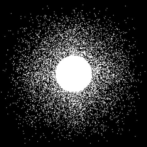
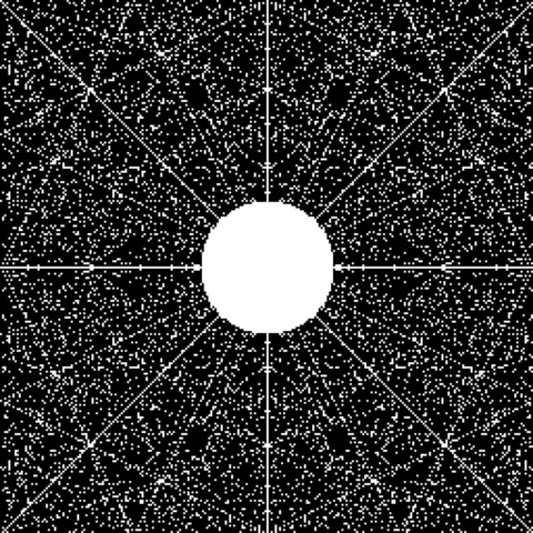
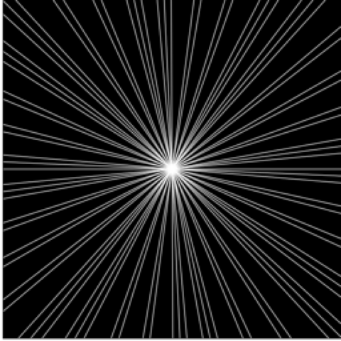
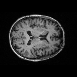
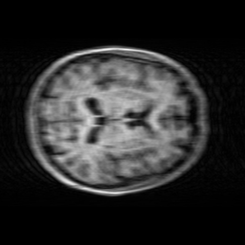
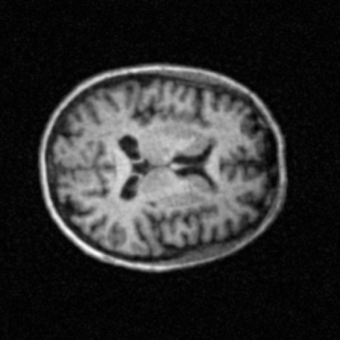
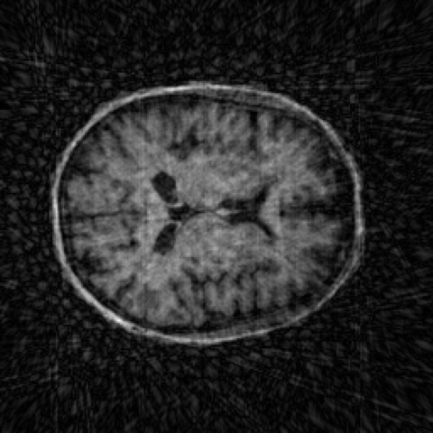
Figure 5: Comparison of different ZF artefacts at 6-fold under-sampling. (left to right): ground, 1D, 2D, p.frac and radial acquisition.

II-G Reconstruction Settings

Our results compare a diverse set of reconstruction algorithms in order to demonstrate the relative performance of p.frac and FCS. Reconstruction algorithms are evaluated according to PSNR and structural similarity (SSIM), with pixel values ranging between [0, 255].

Test inputs are obtained by retroactively under-sampling images and multiplying their $k$-space element-wise with a sampling mask; except in the case of radial acquisition where the Radon transform of the magnitude image is computed. Reverting to image space yields the initial ZF solution (see Figure 5). We choose reduction factors of 2, 4, 6 and 8 to widely vary the difficulty of reconstruction. In practice, constraints limit the precision of the reduction factor, so we choose $R$ to give the closest factor above those stated.

Reconstructions from CS-WV represent a conventional, convex optimisation method for CS-MRI. The wavelet and total variation (TV) terms of the CS-WV algorithm were weighted at $2$ and $6\cdot 10^{-4}$ respectively, indicating reconstructions benefit mostly from TV regularisation and are not as significantly sparse in the wavelet domain. In all cases, 160 iterations were run to yield good performance within a reasonable time; other parameters were the defaults from [20].

To test discrete projective-based reconstruction, we employ FCS via the FFR algorithm and NLM denoising. Knee reconstructions ran for 100 iterations, applying NLM smoothing after every 3. The patch-size ($h$) started at 4, 6, 6, and 6 for 2-, 4-, 6-, and 8-fold reduction respectively. This was then halved after half the iterations and quartered for the last 10%. We found these denoising settings ensured under-sample artefacts were adequately dampened without flattening image features. The choice to reduce $h$ for later iterations is due to the presence of fewer and less pronounced artefacts. Given that the brain images from OASIS-3 presented with more complex structures than the knees dataset, more iterations with lower intensity filtering was opted for to retain high-frequency details. A power curve then regulates $h$ for finer control than was required in the knee reconstructions, with its starting value and curve shape adjusted depending on reduction factor; the curve decays from the initial $h$ value to zero. The starting $h$ values were 4, 2 and 2 for 2-, 4-, and 8-fold under-sampling.

Finally, comparisons against radial acquisition are included. Reconstructions were achieved via simultaneous algebraic reconstruction technique (SART) [60], where magnitude images were used. SART is algorithmically similar to FFR and thus provides insight to reconstruction artefacts that may arise when interpolation is required for projection-based reconstruction. For these experiments we ran 50 iterations, allowing SART to converge for all reduction factors within reasonable time.

The GAN was trained and tested on an NVIDIA P100 GPU. We used the GAN-CS implementation provided by its authors [63]. Based on preliminary experiments and parameters set by [63], our chosen generator architecture cascades 10 copies of one residual block, with its $\ell_{1}$ and $\ell_{2}$ losses weighted 0.95 to 0.05. We trained this for 20 epochs with batch size 2 and learning rate $1\cdot 10^{-5}$, halved every 10,000 iterations with the ADAM optimiser ($\beta_{1}=0.9$).

III Results

(a)     Ground

(b)     CS-WV: 1D

(c)     CS-WV: 2D

(d)     CS-WV: p.frac

(e)     FFR: p.frac

(f)     SART: radial

(g)     Ground

(h)     CS-WV: 1D

(i)     CS-WV: 2D

(j)     CS-WV: p.frac

(k)     FFR: p.frac

(l)     SART: radial

Figure 6: Image quality comparison at 6-fold reduction factor on knee images. Images (a)-(f) are a central slice of the first knee, (g)-(l) are a central slice of the second: (top) magnitude images; (bottom) zoom-in results. Reduced incoherence of 1D Cartesian sampling results in “smearing” of image features.

III-A Comparison of sampling patterns

The distribution of incoherence for p.frac was measured over 1,000 samples using Eq. 3. We select the maximum over ten random $N\times N$ basis matrices equivalent to vectors $\mathbf{e}_{i}$. For comparison, we did the same with 1D and 2D Cartesian random masks. We also compared within each of these: different CTR for the pseudo-random fractal and different polynomial degrees of sampling density $\alpha$ for the Cartesian masks. Table I lists the mean SPR for each under-sampling mask.

Table I: SPR of different pseudo-random sampling operators with various reduction factors (R). Lower value means greater incoherence. p.frac represents pseudo-random fractal sampling, and 1D and 2D random Cartesian sampling.

p.frac		2D Cart.		1D Cart.
R = 2
(CTR=0)	0.014	($\alpha=0$)	0.013	($\alpha=0$)	0.146
(CTR=$N$/12)	0.022	($\alpha=1$)	0.276	($\alpha=1$)	0.312
(CTR=$N$/8)	0.049	($\alpha=2$)	0.354	($\alpha=2$)	0.467
R = 4
(CTR=0)	0.027	($\alpha=0$)	0.022	($\alpha=0$)	0.251
(CTR=$N$/12)	0.065	($\alpha=1$)	0.354	($\alpha=1$)	0.376
(CTR=$N$/8)	0.146	($\alpha=2$)	0.510	($\alpha=2$)	0.561
R = 8
(CTR=0)	0.051	($\alpha=0$)	0.034	($\alpha=0$)	0.382
(CTR=$N$/12)	0.149	($\alpha=1$)	0.384	($\alpha=1$)	0.440
(CTR=$N$/8)	0.350	($\alpha=2$)	0.567	($\alpha=2$)	0.599

With no bias ($\text{CTR}=0$ and $\alpha=0$), 2D Cartesian sampling has the greatest incoherence, closely followed by our proposed sampling. When variable density is introduced the Cartesian masks become far less incoherent. This means the proposed is greatest, even with substantial centre tiling. While SPR is not a comprehensive metric, it is some evidence for the suitability of the proposed sampling pattern.

Figure 5 illustrates how each sampling pattern presents artefacts for a reduction factor of 6. For 1D and 2D random sampling we set $\alpha=2$ to ensure coverage of central $k$-space in a best-case-scenario, as well as CTR equal to that of our randomised fractal for sampling parity. In this figure, 2D random and p.frac under-sampling generate similar artefacts, substantiated by their PSNR and root-mean squared error (RMSE) scores which outperform both 1D and radial trajectories. 1D under-sampling in particular fails to capture much high-frequency detail, with ghosts apparently smearing across the image. It should also be considered that 2D Cartesian sampling is not feasible for MRI in a reasonable time and is primarily included to showcase the best possible outcome for CS. The primary focus in this paper will be to demonstrate the 2D-like performance from FCS and its improvement compared to 1D Cartesian sampling.

III-B Results on complex-valued MRI data

Figure 6 depicts representative knee reconstructions at 6-fold reduction factor. Featured in the comparison are the three solutions from CS-WV, these are 1D and 2D random Cartesian, as well-as p.frac sampling. The FCS and radial reconstructions are also included. We observe that 2D random Cartesian sampling has the best performance of the CS-WV reconstructions, with p.frac outperforming the 1D variant.

Of the projection-based approaches, FCS surpasses radial reconstruction with SART (even considering SART is only reconstructing a magnitude image). We attribute this to the radial reconstruction suffering from the underrepresented transform space, whose artefacts are visible as streaks. Whereas our fractal projects to-and-from DRT space exactly. Figure 7 further strengthens these observations by assessing PSNR and SSIM performance at various reduction factors, showing FCS provides the best results for all reduction factors tested.

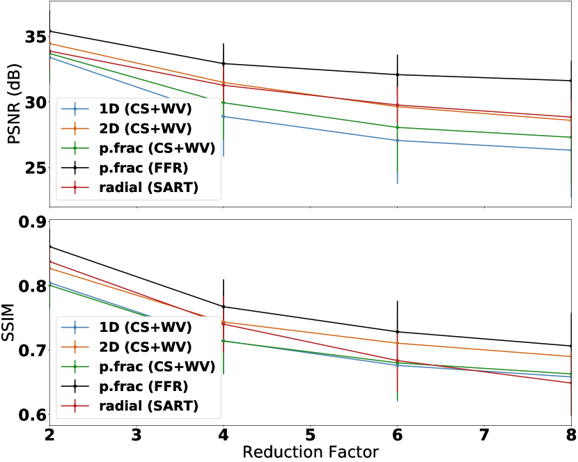
Figure 7: Comparison of the average performance over 182 knee reconstructions for various sampling schemes.

III-C Results on real-valued MRI data

Figure 8 compares the reconstruction performance across the 160 test brain slices for all sampling and reconstruction schemes. Figures 9(a) and 9(b) provide a representative comparison between these techniques for a particularly difficult sample. The slice itself presents with relatively high-frequency detail, whereby the fine ridges of the cerebellum can be difficult to distinguish among under-sample artefacts.

The first three rows of Figure 9(a) contain CS-WV reconstructions for 1D, 2D and p.frac sampling. The fourth row (P-p.frac) additionally compares against an FCS reconstruction using a prime-sized image. Columns (from left-to-right) are 2-, 4- and 8-fold reduction factors. P-p.frac is the optimal choice for this slice at 2-fold undersampling, providing superior PSNR and SSIM scores and achieving a higher overall image quality. At 4- and 8-fold undersampling, 2D with CS-WV is most capable, however both p.frac reconstructions using CS-WV and FCS retain more image features than the 1D CS-WV result. This trend continues for the whole test set (see Figure 8), where any FCS reconstruction can best recover an image at 2-fold undersampling, and all fractal reconstructions consistently beat the 1D solutions.

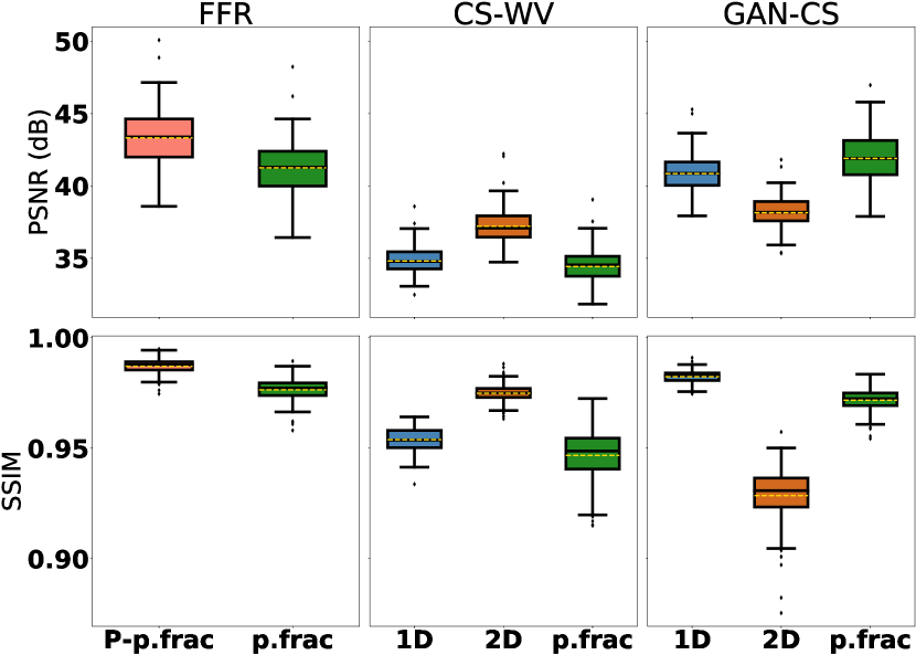
(a) Reduction factor 2

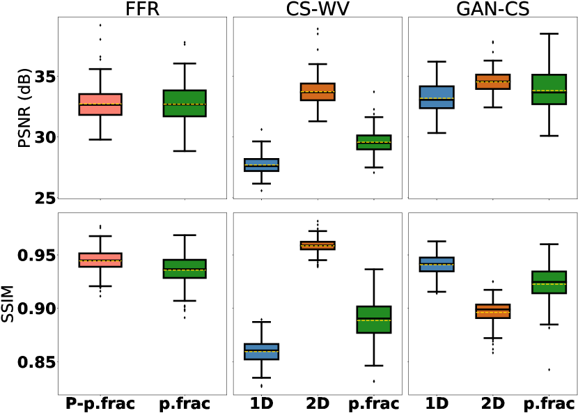
(b) Reduction factor 4

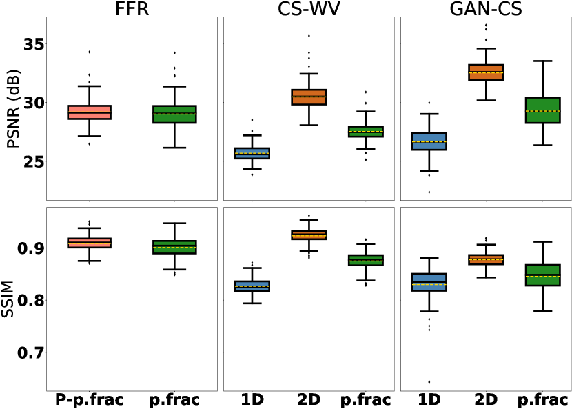
(c) Reduction factor 8

Figure 8: PSNR and SSIM scores for FFR, CS-WV and GAN-CS reconstructions for 160 test subjects of the OASIS-3 dataset at 2-, 4- and 8-fold reduction factors. Yellow dashed line indicates mean performance. P-p.frac indicates use a prime sized image and fractal.

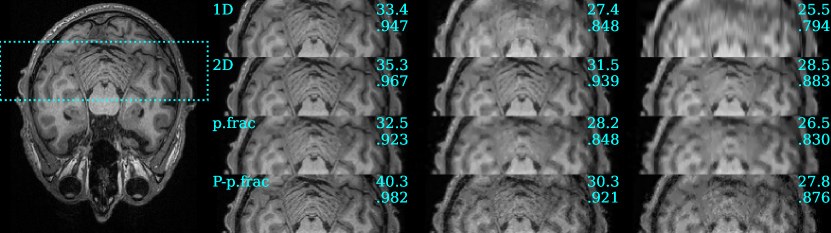
(a) Representative CS-WV and FFR reconstructions of an axial brain MR image, (top to bottom): 1D and 2D Cartesian, pseudo-random fractal (p.frac) and prime-sized p.frac with FFR (P-p.frac); (left to right): ground truth, 2-, 4- and 8-fold under-sampling, overlaid with PSNR (top) and SSIM (bottom).

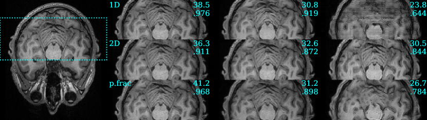
(b) Representative GAN-CS reconstruction of an axial brain MR image, (top to bottom): 1D and 2D Cartesian, pseudo-random fractal (p.frac); (left to right): ground truth, 2-, 4- and 8-fold under-sampling, overlaid with PSNR (top) and SSIM (bottom).

Figure 9: Comparison of different reconstruction algorithms for a representative OASIS-3 brain image.

Figure 9(b) compares GAN-CS reconstructions for 1D, 2D and p.frac sampling. At 2- and 4-fold reduction, all sampling methods perform well, each providing PSNR and SSIM values above 30dB and 0.85 respectively. Visually, images are highly detailed and appropriately recover the cerebellum. In terms of mean PSNR, p.frac sampling outperforms 1D Cartesian sampling at all reduction factors; scoring similarly with SSIM. It isn’t until 8-fold reduction that random 2D Cartesian sampling is clearly superior for image fidelity.

IV Discussion

IV-A Improved Reconstruction Performance

Cartesian random sampling patterns for MR normally only provide 1D incoherence, as measurement hardware is most suitable for linear acquisition and not 2D non-linear trajectories [17]. In this paper, we proposed a method called FCS that uses DRT projections in a pseudo-random fractal (p.frac) pattern, creating 2D incoherence from 1D trajectories. We have shown it provides improved incoherence performance against 1D random Cartesian sampling (Table I) with image artefacts similar in appearance to the 2D variant (Figure 5). Further, the method avoids interpolation normally associated with projection-based trajectories such as radial or spiral while still affording the benefits of orthogonal data collection. Complex-valued knee and amplitude brain MRI are used to demonstrate the performance of FCS in regards to image quality under various reconstruction techniques, with PSNR and SSIM used as metrics to measure image quality. Results with the knee data indicate that p.frac is better suited to CS-WV reconstruction than conventional 1D random acquisition, with PSNR approximately 2dB higher on average at 4-, 6-, and 8-fold reduction over 182 knee images (Figure 7). Additionally, both PSNR and SSIM are highest when our proposed FCS is employed, indicating good convergence to a global minimum from linear optimisation and image filtering. These observations are strengthened by results obtained from the OASIS-3 brain dataset, where p.frac achieved superior image quality under both CS-WV and GAN-CS reconstructions if compared to 1D Cartesian under-sampling (Figure 8). Under these circumstances, FCS reconstructions saw 2D-like reconstruction performance, while also being ideal choice at 2-fold under-sampling. This is also true of the GAN-CS reconstructions, where p.frac enables the highest PSNR scores of all tested sampling patterns at 2-fold reduction.

Figure 10: Comparison between FFR reconstructions using different starting $h$ values for NLM smoothing. Zero-Fill is the 4-fold under-sampled image using the P-p.frac sampling pattern. Reconstructions only differ in the starting $h$ value.

Importantly, while all sampling masks have the same CTR (except for the radial case), it should be noted that both Cartesian 1D and 2D random sampling masks were even more densely captured around central $k$-space. This is due to $\alpha=2$ ensuring that more low-frequency values are selected. In this region, measurements will have a higher PSNR given the tendency of MRI to be focused around the origin. In contrast, FCS is an evenly distributed sampling method, which by design, captures all regions of $k$-space uniformly. It is expected then that reconstructions would favour the 2D random Cartesian sampling as high-frequency, lower PSNR $k$-space is less densely captured. This finding is consistent with the multi-level sampling proposed by [26], which finds optimal sampling conditions when sampling density is decreased as frequency increases. We propose that a multi-level sampling strategy based on DRT projections should be investigated, where low-frequency $k$-space is tiled at a higher density via low-resolution DRT slices. For example, if we consider $N=256$, then we can fully sample all DRT slices for the central $32\times 32$ region and begin to under-sample for $64\times 64$, $128\times 128$ and $256\times 256$. This construction would enable multi-level sampling, whilst adhering to 1D acquisitions at different scales.

IV-B Finite Fourier Reconstruction and Image Filtering

In general, the FFR algorithm used in our FCS performs similarly to CS-WV for 2D random reconstruction, however Figure 10 highlights the susceptibility of NLM to over-filter at higher reduction factors. Zoomed in boxes indicate regions where features have been lost, and where the effect subsequently worsens upon increasing $h$ (patch-size); such behaviour proved difficult to balance for optimal image quality. Similarly at 8-fold reduction, GAN-CS (Figure 9(b)) is only able to recover the cerebellum when 2D random sampling is employed, however instead of flattening this region, the p.frac reconstruction exhibits typical GAN hallucination. Importantly, 1D random reconstructions fail completely, with both the CS-WV and GAN-CS reconstructions unable to recover any significant details of the image. This is reflected in Figure 8 where PSNR scores of p.frac consistently outperform the 1D reconstruction.

While NLM denoising was implemented in this study as-per the $\mathpzc{f}$SIRT algorithm found in [17], similar techniques to FFR [55, 42, 56, 57] have indicated that block-matching and 3D filtering (BM3D) can outperform other denoising algorithms in terms of image quality and computation time for CS applications. Much like NLM, BM3D groups image patches with similar local structures, however, it also jointly denoises each group with a combination of sparsity and filtering techniques. Future work could investigate its suitability for FFR, as well as an incorporation of some techniques used in [42] to fully leverage denoising algorithms for CS applications.

V Conclusion

In this work we introduced a sparse discrete Fourier sampling operator, designed to provide efficient 2D random sampling, showcased with MRI data. Experiments demonstrate that it is suitable for both compressed sensing and projection-based techniques, with FFR seeing reconstruction quality on-par or superior to 2D CS-WV reconstructions. We show knee and brain MRI can be recovered with improved visual fidelity compared to sparse 1D Cartesian sampling, approaching the 2D variant at lower reduction factors—the randomised fractal arguably remains useful up to 8-fold acceleration and GAN-CS reconstruction. Further, the fractal does not suffer from interpolation artefacts that are otherwise observed in radial sampling. These findings are important, as unlike random 2D Cartesian patterns, pseudo-random fractal acquisition can be implemented with 1D sampling characteristics. Future work will investigate a hardware implementation of the proposed acquisition model for MRI, as well-as extending the 2D pseudo-random fractal pattern into a 3D equivalent. The objective will be to develop a fractal-based, rapid MRI acquisition framework, capable of collecting 2D images or 3D volumes.

See pages - of supmat.pdf

References

- [1] E. Candes, J. Romberg, and T. Tao, “Robust uncertainty principles: exact signal reconstruction from highly incomplete frequency information,” IEEE Transactions on Information Theory, vol. 52, no. 2, pp. 489–509, Feb. 2006. [Online]. Available: http://ieeexplore.ieee.org/document/1580791/
- [2] D. Donoho, “Compressed sensing,” IEEE Transactions on Information Theory, vol. 52, no. 4, pp. 1289–1306, Apr. 2006. [Online]. Available: http://ieeexplore.ieee.org/document/1614066/
- [3] M. F. Duarte and Y. C. Eldar, “Structured Compressed Sensing: From Theory to Applications,” IEEE Transactions on Signal Processing, vol. 59, no. 9, pp. 4053–4085, Sep. 2011. [Online]. Available: http://ieeexplore.ieee.org/document/5954192/
- [4] C. G. Graff and E. Y. Sidky, “Compressive sensing in medical imaging,” Applied Optics, vol. 54, no. 8, p. C23, Mar. 2015. [Online]. Available: https://opg.optica.org/abstract.cfm?URI=ao-54-8-C23
- [5] M. Sandilya and S. R. Nirmala, “Compressed sensing trends in magnetic resonance imaging,” Engineering Science and Technology, an International Journal, vol. 20, no. 4, pp. 1342–1352, 2017. [Online]. Available: https://www.sciencedirect.com/science/article/pii/S2215098616313684
- [6] E. J. Candes and T. Tao, “Decoding by linear programming,” IEEE transactions on information theory, vol. 51, no. 12, pp. 4203–4215, 2005, publisher: IEEE.
- [7] ——, “Near-optimal signal recovery from random projections: Universal encoding strategies?” IEEE transactions on information theory, vol. 52, no. 12, pp. 5406–5425, 2006, publisher: IEEE.
- [8] E. J. Candès, “The restricted isometry property and its implications for compressed sensing,” Comptes Rendus Mathematique, vol. 346, no. 9, pp. 589–592, 2008. [Online]. Available: https://www.sciencedirect.com/science/article/pii/S1631073X08000964
- [9] A. Majumdar, Compressed Sensing for Magnetic Resonance Image Reconstruction, 1st ed. Cambridge University Press, Feb. 2015. [Online]. Available: https://www.cambridge.org/core/product/identifier/9781316217795/type/book
- [10] L. Yu, J. P. Barbot, G. Zheng, and H. Sun, “Compressive sensing with chaotic sequence,” IEEE Signal Processing Letters, vol. 17, no. 8, pp. 731–734, 2010, publisher: IEEE.
- [11] N. Linh-Trung, D. Van Phong, Z. M. Hussain, H. T. Huynh, V. L. Morgan, and J. C. Gore, “Compressed sensing using chaos filters,” in 2008 Australasian Telecommunication Networks and Applications Conference. IEEE, 2008, pp. 219–223.
- [12] V. Kafedziski and T. Stojanovski, “Compressive sampling with chaotic dynamical systems,” in 2011 19th Telecommunications Forum (TELFOR) Proceedings of Papers. IEEE, 2011, pp. 695–698.
- [13] L. Zeng, X. Zhang, L. Chen, T. Cao, and J. Yang, “Deterministic construction of toeplitzed structurally chaotic matrix for compressed sensing,” Circuits, Systems, and Signal Processing, vol. 34, pp. 797–813, 2015, publisher: Springer.
- [14] D. Rontani, D. Choi, C.-Y. Chang, A. Locquet, and D. Citrin, “Compressive sensing with optical chaos,” Scientific reports, vol. 6, no. 1, pp. 1–7, 2016, publisher: Springer.
- [15] H. Gan, S. Xiao, Y. Zhao, and X. Xue, “Construction of efficient and structural chaotic sensing matrix for compressive sensing,” Signal Processing: Image Communication, vol. 68, pp. 129–137, 2018, publisher: Elsevier.
- [16] H. Gan, S. Xiao, and Y. Zhao, “A large class of chaotic sensing matrices for compressed sensing,” Signal Processing, vol. 149, pp. 193–203, 2018, publisher: Elsevier.
- [17] S. S. Chandra, G. Ruben, J. Jin, M. Li, A. M. Kingston, I. D. Svalbe, and S. Crozier, “Chaotic Sensing,” IEEE Transactions on Image Processing, vol. 27, no. 12, pp. 6079–6092, Dec. 2018. [Online]. Available: https://ieeexplore.ieee.org/document/8432445/
- [18] H. Gan, S. Xiao, and F. Liu, “Chaotic binary sensing matrices,” International Journal of Bifurcation and Chaos, vol. 29, no. 09, p. 1950121, 2019, publisher: World Scientific.
- [19] H. Gan, S. Xiao, T. Zhang, and F. Liu, “Bipolar measurement matrix using chaotic sequence,” Communications in Nonlinear Science and Numerical Simulation, vol. 72, pp. 139–151, 2019, publisher: Elsevier.
- [20] M. Lustig, D. Donoho, and J. M. Pauly, “Sparse MRI: The application of compressed sensing for rapid MR imaging,” Magnetic Resonance in Medicine, vol. 58, no. 6, pp. 1182–1195, Dec. 2007. [Online]. Available: https://onlinelibrary.wiley.com/doi/10.1002/mrm.21391
- [21] S. Geethanath, R. Reddy, A. S. Konar, S. Imam, R. Sundaresan, R. B. D. R., and R. Venkatesan, “Compressed Sensing MRI: A Review,” Critical Reviews in Biomedical Engineering, vol. 41, no. 3, pp. 183–204, 2013. [Online]. Available: http://www.dl.begellhouse.com/journals/4b27cbfc562e21b8,4863d6072e2ac4d2,006a9a9a2463d112.html
- [22] J. C. Ye, “Compressed sensing MRI: a review from signal processing perspective,” BMC Biomedical Engineering, vol. 1, no. 1, p. 8, Dec. 2019.
- [23] M. Lustig, D. Donoho, J. Santos, and J. Pauly, “Compressed Sensing MRI,” IEEE Signal Processing Magazine, vol. 25, no. 2, pp. 72–82, Mar. 2008. [Online]. Available: http://ieeexplore.ieee.org/document/4472246/
- [24] M. Seeger, H. Nickisch, R. Pohmann, and B. Schölkopf, “Optimization of k -space trajectories for compressed sensing by Bayesian experimental design: Bayesian Optimization of k -Space Trajectories,” Magnetic Resonance in Medicine, vol. 63, no. 1, pp. 116–126, Jan. 2010. [Online]. Available: https://onlinelibrary.wiley.com/doi/10.1002/mrm.22180
- [25] F. Krahmer and R. Ward, “Stable and Robust Sampling Strategies for Compressive Imaging,” IEEE Transactions on Image Processing, vol. 23, no. 2, pp. 612–622, Feb. 2014. [Online]. Available: http://ieeexplore.ieee.org/document/6651836/
- [26] B. Adcock, A. C. Hansen, C. Poon, and B. Roman, “BREAKING THE COHERENCE BARRIER: A NEW THEORY FOR COMPRESSED SENSING,” Forum of Mathematics, Sigma, vol. 5, p. e4, 2017. [Online]. Available: https://www.cambridge.org/core/product/identifier/S2050509416000323/type/journal_article
- [27] H. Wang, D. Liang, and L. Ying, “Pseudo 2D random sampling for compressed sensing MRI,” in 2009 Annual International Conference of the IEEE Engineering in Medicine and Biology Society. IEEE, 2009, pp. 2672–2675.
- [28] D. Tamada and K. Kose, “Two-dimensional compressed sensing using the cross-sampling approach for low-field MRI systems,” IEEE transactions on medical imaging, vol. 33, no. 9, pp. 1905–1912, 2014, publisher: IEEE.
- [29] Y. Yang, F. Liu, Z. Jin, and S. Crozier, “Aliasing Artefact Suppression in Compressed Sensing MRI for Random Phase-Encode Undersampling,” IEEE Transactions on Biomedical Engineering, vol. 62, no. 9, pp. 2215–2223, Sep. 2015. [Online]. Available: http://ieeexplore.ieee.org/document/7078916/
- [30] K. T. Block, M. Uecker, and J. Frahm, “Undersampled radial MRI with multiple coils. Iterative image reconstruction using a total variation constraint,” Magnetic Resonance in Medicine, vol. 57, no. 6, pp. 1086–1098, Jun. 2007. [Online]. Available: https://onlinelibrary.wiley.com/doi/10.1002/mrm.21236
- [31] J. C. Ye, S. Tak, Y. Han, and H. W. Park, “Projection reconstruction MR imaging using FOCUSS,” Magnetic Resonance in Medicine, vol. 57, no. 4, pp. 764–775, Apr. 2007. [Online]. Available: https://onlinelibrary.wiley.com/doi/10.1002/mrm.21202
- [32] H. Jung, J. Park, J. Yoo, and J. C. Ye, “Radial k-t FOCUSS for high-resolution cardiac cine MRI: Radial k-t FOCUSS Cardiac Cine Imaging,” Magnetic Resonance in Medicine, vol. 63, no. 1, pp. 68–78, Jan. 2010. [Online]. Available: https://onlinelibrary.wiley.com/doi/10.1002/mrm.22172
- [33] L. Feng, R. Grimm, K. T. Block, H. Chandarana, S. Kim, J. Xu, L. Axel, D. K. Sodickson, and R. Otazo, “Golden-angle radial sparse parallel MRI: Combination of compressed sensing, parallel imaging, and golden-angle radial sampling for fast and flexible dynamic volumetric MRI: iGRASP: Iterative Golden-Angle RAdial Sparse Parallel MRI,” Magnetic Resonance in Medicine, vol. 72, no. 3, pp. 707–717, Sep. 2014. [Online]. Available: https://onlinelibrary.wiley.com/doi/10.1002/mrm.24980
- [34] G. H. Glover and D. C. Noll, “Consistent projection reconstruction (CPR) techniques for MRI,” Magnetic Resonance in Medicine, vol. 29, no. 3, pp. 345–351, Mar. 1993. [Online]. Available: https://onlinelibrary.wiley.com/doi/10.1002/mrm.1910290310
- [35] T. P. Trouard, Y. Sabharwal, M. I. Altbach, and A. F. Gmitro, “Analysis and comparison of motion-correction techniques in diffusion-weighted imaging,” Journal of Magnetic Resonance Imaging, vol. 6, no. 6, pp. 925–935, Nov. 1996. [Online]. Available: https://onlinelibrary.wiley.com/doi/10.1002/jmri.1880060614
- [36] M. Katoh, E. Spuentrup, A. Buecker, W. J. Manning, R. W. Günther, and R. M. Botnar, “MR coronary vessel wall imaging: Comparison between radial and spiral k-space sampling,” Journal of Magnetic Resonance Imaging, vol. 23, no. 5, pp. 757–762, May 2006. [Online]. Available: https://onlinelibrary.wiley.com/doi/10.1002/jmri.20569
- [37] Q. H. Liu and N. Nguyen, “Nonuniform fast Fourier transform (NUFFT) algorithm and its applications,” in IEEE Antennas and Propagation Society International Symposium. 1998 Digest. Antennas: Gateways to the Global Network. Held in conjunction with: USNC/URSI National Radio Science Meeting (Cat. No.98CH36, vol. 3, 1998, pp. 1782–1785 vol.3.
- [38] Jiayu Song, Yanhui Liu, S. Gewalt, G. Cofer, G. Johnson, and Qing Huo Liu, “Least-Square NUFFT Methods Applied to 2-D and 3-D Radially Encoded MR Image Reconstruction,” IEEE Transactions on Biomedical Engineering, vol. 56, no. 4, pp. 1134–1142, Apr. 2009. [Online]. Available: http://ieeexplore.ieee.org/document/4760269/
- [39] A. K. Louis and W. Törnig, “Ghosts in tomography - the null space of the radon transform,” Mathematical Methods in the Applied Sciences, vol. 3, no. 1, pp. 1–10, 1981. [Online]. Available: https://onlinelibrary.wiley.com/doi/10.1002/mma.1670030102
- [40] Y. Yang, F. Liu, M. Li, J. Jin, E. Weber, Q. Liu, and S. Crozier, “Pseudo-Polar Fourier Transform-Based Compressed Sensing MRI,” IEEE Transactions on Biomedical Engineering, vol. 64, no. 4, pp. 816–825, Apr. 2017. [Online]. Available: http://ieeexplore.ieee.org/document/7488260/
- [41] A. Averbuch, R. R. Coifman, D. L. Donoho, M. Israeli, and Y. Shkolnisky, “A Framework for Discrete Integral Transformations I—The Pseudopolar Fourier Transform,” SIAM Journal on Scientific Computing, vol. 30, no. 2, pp. 764–784, Jan. 2008. [Online]. Available: http://epubs.siam.org/doi/10.1137/060650283
- [42] C. A. Metzler, A. Maleki, and R. G. Baraniuk, “From Denoising to Compressed Sensing,” IEEE Transactions on Information Theory, vol. 62, no. 9, pp. 5117–5144, Sep. 2016.
- [43] S. Ravishankar and Y. Bresler, “MR Image Reconstruction From Highly Undersampled k-Space Data by Dictionary Learning,” IEEE Transactions on Medical Imaging, vol. 30, no. 5, pp. 1028–1041, May 2011. [Online]. Available: http://ieeexplore.ieee.org/document/5617283/
- [44] X. Qu, Y. Hou, F. Lam, D. Guo, J. Zhong, and Z. Chen, “Magnetic resonance image reconstruction from undersampled measurements using a patch-based nonlocal operator,” Medical Image Analysis, vol. 18, no. 6, pp. 843–856, 2014. [Online]. Available: https://www.sciencedirect.com/science/article/pii/S1361841513001448
- [45] W. Dong, G. Shi, X. Li, Y. Ma, and F. Huang, “Compressive Sensing via Nonlocal Low-Rank Regularization,” IEEE Transactions on Image Processing, vol. 23, no. 8, pp. 3618–3632, Aug. 2014. [Online]. Available: http://ieeexplore.ieee.org/document/6827224/
- [46] S. Ravishankar and Y. Bresler, “Sparsifying transform learning for Compressed Sensing MRI,” in 2013 IEEE 10th International Symposium on Biomedical Imaging. San Francisco, CA, USA: IEEE, Apr. 2013, pp. 17–20. [Online]. Available: http://ieeexplore.ieee.org/document/6556401/
- [47] B. Wen, Y. Li, and Y. Bresler, “Image Recovery via Transform Learning and Low-Rank Modeling: The Power of Complementary Regularizers,” IEEE Transactions on Image Processing, vol. 29, pp. 5310–5323, 2020. [Online]. Available: https://ieeexplore.ieee.org/document/9042815/
- [48] Z. Zhan, J.-F. Cai, D. Guo, Y. Liu, Z. Chen, and X. Qu, “Fast Multiclass Dictionaries Learning With Geometrical Directions in MRI Reconstruction,” IEEE Transactions on Biomedical Engineering, vol. 63, no. 9, pp. 1850–1861, Sep. 2016. [Online]. Available: http://ieeexplore.ieee.org/document/7337391/
- [49] B. Wen, S. Ravishankar, L. Pfister, and Y. Bresler, “Transform Learning for Magnetic Resonance Image Reconstruction: From Model-Based Learning to Building Neural Networks,” IEEE Signal Processing Magazine, vol. 37, no. 1, pp. 41–53, Jan. 2020. [Online]. Available: https://ieeexplore.ieee.org/document/8962391/
- [50] K. P. Pruessmann, M. Weiger, M. B. Scheidegger, and P. Boesiger, “SENSE: Sensitivity encoding for fast MRI,” Magnetic Resonance in Medicine, vol. 42, no. 5, pp. 952–962, 1999. [Online]. Available: https://onlinelibrary.wiley.com/doi/abs/10.1002/%28SICI%291522-2594%28199911%2942%3A5%3C952%3A%3AAID-MRM16%3E3.0.CO%3B2-S
- [51] M. A. Griswold, P. M. Jakob, M. Nittka, J. W. Goldfarb, and A. Haase, “Partially parallel imaging with localized sensitivities (PILS),” Magnetic Resonance in Medicine, vol. 44, no. 4, pp. 602–609, Oct. 2000. [Online]. Available: https://onlinelibrary.wiley.com/doi/10.1002/1522-2594(200010)44:4<602::AID-MRM14>3.0.CO;2-5
- [52] M. A. Griswold, P. M. Jakob, R. M. Heidemann, M. Nittka, V. Jellus, J. Wang, B. Kiefer, and A. Haase, “Generalized autocalibrating partially parallel acquisitions (GRAPPA),” Magnetic Resonance in Medicine, vol. 47, no. 6, pp. 1202–1210, Jun. 2002. [Online]. Available: https://onlinelibrary.wiley.com/doi/10.1002/mrm.10171
- [53] D. K. Sodickson and W. J. Manning, “Simultaneous acquisition of spatial harmonics (SMASH): Fast imaging with radiofrequency coil arrays,” Magnetic Resonance in Medicine, vol. 38, no. 4, pp. 591–603, Oct. 1997. [Online]. Available: https://onlinelibrary.wiley.com/doi/10.1002/mrm.1910380414
- [54] F. Matus and J. Flusser, “Image representation via a finite Radon transform,” IEEE Transactions on Pattern Analysis and Machine Intelligence, vol. 15, no. 10, pp. 996–1006, Oct. 1993. [Online]. Available: http://ieeexplore.ieee.org/document/254058/
- [55] J. Tan, Y. Ma, and D. Baron, “Compressive imaging via approximate message passing with wavelet-based image denoising,” in 2014 IEEE Global Conference on Signal and Information Processing (GlobalSIP). Atlanta, GA, USA: IEEE, Dec. 2014, pp. 424–428. [Online]. Available: http://ieeexplore.ieee.org/document/7032152/
- [56] E. M. Eksioglu, “Decoupled Algorithm for MRI Reconstruction Using Nonlocal Block Matching Model: BM3D-MRI,” Journal of Mathematical Imaging and Vision, vol. 56, no. 3, pp. 430–440, Nov. 2016. [Online]. Available: http://link.springer.com/10.1007/s10851-016-0647-7
- [57] E. M. Eksioglu and A. K. Tanc, “Denoising AMP for MRI Reconstruction: BM3D-AMP-MRI,” SIAM Journal on Imaging Sciences, vol. 11, no. 3, pp. 2090–2109, 2018. [Online]. Available: https://doi.org/10.1137/18M1169655
- [58] G. Ou, D. Lun, and B. Ling, “Compressive sensing of images based on discrete periodic Radon transform,” Electronics Letters, vol. 50, no. 8, pp. 591–593, Apr. 2014. [Online]. Available: https://onlinelibrary.wiley.com/doi/10.1049/el.2014.0770
- [59] A. Kingston and I. Svalbe, “Generalised finite Radon transform for N×N images,” Image and Vision Computing, vol. 25, no. 10, pp. 1620–1630, Oct. 2007. [Online]. Available: https://linkinghub.elsevier.com/retrieve/pii/S0262885606001119
- [60] A. C. Kak and M. Slaney, Principles of Computerized Tomographic Imaging. Society for Industrial and Applied Mathematics, 2001, _eprint: https://epubs.siam.org/doi/pdf/10.1137/1.9780898719277. [Online]. Available: https://epubs.siam.org/doi/abs/10.1137/1.9780898719277
- [61] G. H. Hardy and E. M. Wright, An Introduction to the Theory of Numbers, 4th ed. Oxford, 1975.
- [62] S. S. Chandra, N. Normand, A. Kingston, J. Guédon, and I. Svalbe, “Robust digital image reconstruction via the discrete fourier slice theorem,” IEEE Signal Processing Letters, vol. 21, no. 6, pp. 682–686, 2014.
- [63] M. Mardani, E. Gong, J. Y. Cheng, S. S. Vasanawala, G. Zaharchuk, L. Xing, and J. M. Pauly, “Deep Generative Adversarial Neural Networks for Compressive Sensing MRI,” IEEE Transactions on Medical Imaging, vol. 38, no. 1, pp. 167–179, Jan. 2019. [Online]. Available: https://ieeexplore.ieee.org/document/8417964/
- [64] K. He, X. Zhang, S. Ren, and J. Sun, “Deep Residual Learning for Image Recognition,” in 2016 IEEE Conference on Computer Vision and Pattern Recognition (CVPR). Las Vegas, NV, USA: IEEE, Jun. 2016, pp. 770–778. [Online]. Available: http://ieeexplore.ieee.org/document/7780459/
- [65] D. Liang, J. Cheng, Z. Ke, and L. Ying, “Deep Magnetic Resonance Image Reconstruction: Inverse Problems Meet Neural Networks,” IEEE Signal Processing Magazine, vol. 37, no. 1, pp. 141–151, 2020.
- [66] S. S. Chandra, M. Bran Lorenzana, X. Liu, S. Liu, S. Bollmann, and S. Crozier, “Deep learning in magnetic resonance image reconstruction,” Journal of Medical Imaging and Radiation Oncology, vol. 65, no. 5, pp. 564–577, Aug. 2021. [Online]. Available: https://onlinelibrary.wiley.com/doi/10.1111/1754-9485.13276
- [67] A. M. Sawyer, M. Lustig, M. Alley, P. Uecker, P. Virtue, P. Lai, S. Vasanawala, and G. Healthcare, “Creation of Fully Sampled MR Data Repository for Compressed Sensing of the Knee.”
- [68] P. J. LaMontagne, T. L. Benzinger, J. C. Morris, S. Keefe, R. Hornbeck, C. Xiong, E. Grant, J. Hassenstab, K. Moulder, A. G. Vlassenko, M. E. Raichle, C. Cruchaga, and D. Marcus, “OASIS-3: Longitudinal Neuroimaging, Clinical, and Cognitive Dataset for Normal Aging and Alzheimer Disease,” Dec. 2019, publisher: Cold Spring Harbor Laboratory.