Cai, Chen, Wainwright, and Zhao

Doubly High-Dimensional Contextual Bandits

Doubly High-Dimensional Contextual Bandits:
An Interpretable Model for Joint Assortment-Pricing

Junhui Cai Department of Information Technology, Analytics, and Operations, University of Notre Dame, jcai2@nd.edu Ran Chen Laboratory for Information and Decision Systems, Massachusetts Institute of Technology, ran1chen@mit.edu Martin J. Wainwright Laboratory for Information and Decision Systems, Statistics and Data Science Center,
EECS & Mathematics, Massachusetts Institute of Technology, wainwrigwork@gmail.com Linda Zhao Department of Statistics and Data Science, University of Pennsylvania, lzhao@wharton.upenn.edu

Key challenges in running a retail business include how to select products to present to consumers (the assortment problem), and how to price products (the pricing problem) to maximize revenue or profit. Instead of considering these problems in isolation, we propose a joint approach to assortment-pricing based on contextual bandits. Our model is doubly high-dimensional, in that both context vectors and actions are allowed to take values in high-dimensional spaces. In order to circumvent the curse of dimensionality, we propose a simple yet flexible model that captures the interactions between covariates and actions via a (near) low-rank representation matrix. The resulting class of models is reasonably expressive while remaining interpretable through latent factors, and includes various structured linear bandit and pricing models as particular cases. We propose a computationally tractable procedure that combines an exploration/exploitation protocol with an efficient low-rank matrix estimator, and we prove bounds on its regret. Simulation results show that this method has lower regret than state-of-the-art methods applied to various standard bandit and pricing models. Real-world case studies on the assortment-pricing problem, from an industry-leading instant noodles company to an emerging beauty start-up, underscore the gains achievable using our method. In each case, we show at least three-fold gains in revenue or profit by our bandit method, as well as the interpretability of the latent factor models that are learned.

contextual bandits; on-line decision-making; high-dimensional statistics; low-rank matrices; factor models.

1 Introduction

In the modern business and healthcare landscape, it is now status quo to make use of online decision-making algorithms that incorporate individual characteristics as well as micro- and macro-economic factors. For example, on-line retailers determine product offerings and pricing based on customer demographics, browsing, and purchasing history; business managers allocate resources, such as staff and equipment, based on current operational conditions; and medical providers prescribe treatment and therapy combinations based on the patient’s medical records.

In these settings, bandit algorithms are often deployed to learn the reward structure while optimizing performance by strategically “exploring” and “exploiting” potential actions. In order to make optimal decisions, the decision-maker must take into account two factors: the reward (e.g., revenue or profit) depends on both a space of possible actions, as well as individual features or covariates, also known as the context. Many bandit algorithms are limited to finite or relatively low-dimensional action and context spaces, but in practice, both can be high-dimensional in nature. For instance, the action vector for an online retailer may include pricing and assortment information for thousands of products. Thus, we are led to consider the following question: can we develop useful models and efficient learning procedures for contextual bandits that are high-dimensional in both actions and covariates? Providing one affirmative answer to this open question—and demonstrating the utility of the resulting model and algorithms for two real-world motivating case studies—are the primary contributions of our work.

1.1 Background and Our Approach

The primary application that motivates our work is dynamic assortment and pricing. It is a central challenge for on-line retailers, and using bandits for this problem is natural given the sequential nature of the decision-making. The assortment problem amounts to choosing the selection of products to be offered while satisfying capacity constraints, whereas the pricing problem is to set selling prices for these products. Both assortment and pricing decisions share a common goal: maximizing a specific objective function, such as revenue or profit. Although both dynamic assortment optimization and pricing problems have been separately studied extensively in the literature, the joint assortment-pricing problem has received comparatively less attention.

The key to a successful assortment and pricing strategy lies in understanding market response to the assortment-pricing decisions. A major challenge in modern assortment-pricing is the explosion in dimensionality of both the action and covariate spaces. Companies typically consider large numbers ($\gg 100$) of products simultaneously. From the universe of products, they consider large collections of possible product subsets to display, and the associated price takes values in continuous space. Thus, the action space becomes high-dimensional with a mixture of discrete and continuous elements. The problem is further complicated by the high-dimensional covariates: fueled by the rise of e-commerce, it is possible to measure many customer-specific or industry-specific features that can be relevant to modeling demand and price sensitivity. As the action-covariate dimensions grow, without some kind of structure, there are “no-free-lunch” theorems showing that it is prohibitively costly, both in terms of samples and computation, to learn an optimal policy (Lattimore and Szepesvári, 2020). Thus, it becomes essential to develop models with “low-dimensional structure” that explain important features of the data, while being amenable to statistically and computationally efficient algorithms.

A fortunate fact—and the starting point for our modeling—is that there often exist low-dimensional latent factors that explain the bulk of the reward structure. In the retail context, the demands for products, one deciding quantity for the reward, that share similar features/attributes are influenced in common ways by underlying market features. And usually only a handful of the underlying product factors matter. For instance, there exists “color psychology” in marketing (Singh, 2006) and customers’ color preference in basic colors such as white, black, blue, and red (Madden et al., 2000). Similarly, the covariate vectors relevant for assortment-pricing can be explained by a few latent factors. For instance, at the individual level, much of the variance in consumer buying power can be captured by a mixture of demographic (e.g., income, education level) and geographic traits (see Pol, (1991) and references therein); at the macro level, population purchasing preference, usually indicated by season, region, and other macroeconomic indices, significantly impact the overall demand (Estelami et al., 2001, Gordon et al., 2013, Kumar et al., 2014). As a result, the interaction effects between the action and covariates—a major source contributing to revenue generation—can be characterized by a few latent factors. For example, customers with lower buying power tend be more conservative in their buying behavior (e.g., (Wakefield and Inman, 2003)).

In summary, the low-dimensional structure, therefore, captures the essence of the effect of actions and covariates on the reward function and often aligns with intuitive or interpretable factors. Accounting for the common latent factors further speeds up the reward learning per product and low-dimensional models often improve computational efficiency. The interpretability and computational efficiency using latent factors turn the “curse of dimensionality” into a “blessing of dimensionality” (Li et al., 2018).

With these insights, we tackle the joint assortment-pricing problem by casting it as a doubly high-dimensional bandit problem and propose a new model that captures interactions between the high-dimensional actions and covariates via an (approximately) low-rank matrix representation. Our goal is to offer a sequence of assortment and pricing decisions, which can be represented as a sequence of action vectors $\{{\bm{a}}_{t}\}_{t=1}^{T}$ that take values in (some subset of) ${}^{d_{a}}$, under the contexts, which can be represented as a sequence of covariate vectors $\{{\bm{x}}_{t}\}_{t=1}^{T}$ taking values in ${}^{d_{x}}$, such that the cumulative expected revenue over the time horizon $T$ is maximized. Since both the action dimension $d_{a}$ and the covariate dimension $d_{x}$ can be large, our proposed model uses a low-rank matrix to take advantage of the low-dimensional latent factors. Specifically, our reward model takes the bilinear form: given an action vector ${\bm{a}}\in\mathbb{R}^{d_{a}}$ and a covariate vector ${\bm{x}}\in\mathbb{R}^{d_{x}}$, we observe a noisy reward $Y$ with conditional mean

$$\mathbb{E}[Y\mid{\bm{x}},{\bm{a}}]={\bm{a}}^{T}{\bm{\Theta}}^{*}{\bm{x}},$$

where ${\bm{\Theta}}^{*}\in\mathbb{R}^{d_{a}\times d_{x}}$ is an unknown representation matrix that is relatively low-rank—say with rank $r\ll\min\{d_{a},d_{x}\}$—or more generally, well-approximated by a matrix with low rank.

The representation matrix ${\bm{\Theta}}^{*}$ captures important interactions between actions and covariate pairs via its spectral structure. Performing a singular value decomposition (SVD) on the representation matrix yields the latent structure, with the left (respectively right) singular vectors corresponding to the action (respectively covariate) space structure. In this way, our model implicitly performs a form of dimension reduction in how the actions and covariates interact to determine the reward function.

Given this structure, we also propose a new algorithm (Hi-CCAB) that combines low-rank estimation with an exploration/exploitation strategy. It is a computationally efficient approach, involving only the solution of simple convex programs in all phases. We prove non-asymptotic bound on its expected regret, one that shows that it is also statistically efficient in terms of problem dimension and structure. We also show our method not only can solve the joint assortment-pricing problem, but is actually general enough to encompass various bandit models as special cases.

1.2 Main Contributions

Let us summarize some of our main contributions:

1. A general and interpretable model for joint assortment-pricing: We propose a new model for doubly high-dimensional contextual bandits, in which both covariates and actions can be high-dimensional and continuous, by leveraging the low-dimensional latent factors using a low-rank representation matrix. We then adopt our new model to tackle the joint dynamic assortment-pricing problem, which allows for feature-dependent and context-specific demand heterogeneity, while previous literature mostly studies the assortment and pricing problems separately. In addition, our model can account for new products as opposed to a predetermined set of available products in most existing assortment models.

   As we argue, an advantage of this low-rank model is its combination of a high degree of interpretability with prediction power. The low-rank matrix encapsulates the interaction between action-covariate pairs via its singular vectors, providing a form of dimension reduction and interpretability. On the other hand, given the covariate, our model is able to predict the reward of an unseen arm. Both interpretability and predictive power can be tremendously useful for decision-makers.

   Our model is general. It unifies a number of structured bandit and pricing models studied in past work; it can capture complex relationships between variables; and it is applicable to an array of applications involving multiple decision-making.

2. An computationally efficient and adaptive algorithm. We propose an efficient algorithm for online learning, referred to as the High-dimensional Contextual and High-dimensional Continumm Armed Bandit (Hi-CCAB). It interleaves estimation steps, in which the low-rank representation matrix is estimated based on data observed thus far, with exploration/exploitation steps, in which new actions are selected. Unlike explore-then-commit type algorithms, Hi-CCAB is adaptive with respect to the time horizon $T$: in particular, there are no $T$-dependent tuning parameters (e.g., exploration period). Moreover, it updates the representation matrix across the entire time horizon, making it more suitable for online learning. On a separate note, it is also adaptive to the rank $r$ (i.e., the number of latent factors) in that it does not require prior knowledge of $r$.

3. A non-asymptotic and instance-dependent upper bound. We measure the performance of our algorithm using the standard notion of expected regret, which is the average expected deficit in reward achieved by Hi-CCAB compared with an oracle that knows the low-rank representation matrix. We provide a non-asymptotic upper bound on the expected regret of Hi-CCAB. The technical challenge is that samples are not i.i.d because the bandit protocol during the exploitation step adaptively collects samples, making classic matrix theory results for i.i.d. data inapplicable. We overcome this challenge by proving a new tail bound for the low-rank matrix estimator by carefully leveraging empirical process and martingales concentration results, and thereby a non-asymptotic upper bound on the expected regret. We further note that the non-asymptotic bounds hold for all $T$ while the algorithm does not require prior knowledge of $T$. This adaptivity is of both theoretical interest and practical importance.

4. Take-away insights for assortment-pricing practice. We compare the performance of Hi-CCAB against existing algorithms under various standard bandit and pricing models and applications to real-world retail problems. Simulations demonstrate that Hi-CCAB outperforms state-of-the-art methods in expected regret. We further apply Hi-CCAB to two real-world retail problems involving joint assortment and pricing, one for a leading instant noodle producer and the other for a manicure start-up. The results demonstrate the effectiveness of this joint approach for revenue maximization. Both case studies involve a large number of products and covariates and no existing methods are applicable. Hi-CCAB is shown to be capable of managing such doubly high dimensionalities and providing simultaneous assortment and pricing decisions. The assortment-pricing policy based on Hi-CCAB yields sales almost four times as high as the strategies in practice. Moreover, our model reveals insights for assortment and pricing such as the popularity of flavor (noodles) or color (manicure) under different contexts such as locations and seasons. Finally, our model is able to predict the revenue of a new product, which can guide new product designs.

1.3 Related Literature

So as to situate our work more broadly, let discuss and summarize some related literature.

Dynamic Assortment and Pricing.

In the field of operations research and revenue management, assortment and pricing are key decisions to be made by any firm; accordingly, there is a substantial body of past work on dynamic assortment and dynamic pricing.

Beginning with dynamic assortment, Caro and Gallien, (2007) was an early approach to formulate it as a multi-armed bandit problem, but assuming independent demand for each product. A popular alternative demand model is the multinomial logit (MNL) choice model, which uses a logistic model to estimate demand parameters (Rusmevichientong et al., 2010, Sauré and Zeevi, 2013); more recent work has adapted multi-arm bandit techniques to the MNL model (Chen and Wang, 2017, Agrawal et al., 2019, Chen et al., 2021, 2023). The MNL model can be further extended for personalization dynamic assortment by integrating personal information (Cheung and Simchi-Levi, 2017, Chen et al., 2020, Miao and Chao, 2022). Another MNL variant accounts for heterogeneity via customer segmentation (Bernstein et al., 2019, Kallus and Udell, 2020). In particular, Kallus and Udell, (2020) also adopt a low-rank matrix to model the interaction between product and customer types, but they only consider finite types of products and customers and does not account for product/customer attributes. Apart from estimating the optimal set, recently Shen et al., (2023) propose the first inferential framework for testing optimal assortment. It is worth mentioning two limitations on the MNL model. First, the unit of the MNL model is limited to one customer arrival, so does not capture the dynamic nature of customer arrivals. These dynamics have significant impacts on decisions taken over extended periods like weeks, months, and years. Our model, on the other hand, directly models the revenue itself and can be adopted at any granularity. At the customer level, we do not assume each customer only purchases one of the products offered, which is usually not the case in practice. Second, MNL models treat each product in isolation, ignoring any inherent product similarities. Our model leverages product attributes to capture product similarities. As a result, our model can improve predictive power and provide deeper insights. Moreover, it can further handle new products while the set of available products is predetermined in the MNL models.

Dynamic pricing has been another important stream in revenue management and the price-demand curve is often assumed to be linear (Kleinberg and Leighton, 2003, Araman and Caldentey, 2009, Besbes and Zeevi, 2009, Broder and Rusmevichientong, 2012, den Boer and Zwart, 2014, Keskin and Zeevi, 2014); the paper by Den Boer, (2015) provides a helpful survey. Recent work has turned towards dynamic pricing based on customer characteristics (e.g., Ban and Keskin, (2021), Chen and Gallego, (2021), Bastani et al., (2022)) and/or product features (e.g., Qiang and Bayati, (2016), Javanmard and Nazerzadeh, (2019), Cohen et al., (2020), Miao et al., (2022), Fan et al., (2022)). Much of the pricing literature focuses on the single-product setting, while sellers usually need to price multiple products simultaneously. The MNL model has also been used in multi-product pricing problem (Akçay et al., 2010, Gallego and Wang, 2014) but they do not consider product feature or customer characteristics. The recent work of Bastani et al., (2022) proposes a meta-dynamic pricing algorithm, which uses an empirical Bayes approach to learn the demand function across products by assuming that the demand parameters of each product follow a common unknown prior to leveraging the similarities in demand among related products. However, their algorithm learns products sequentially, while our algorithm provides pricing for multi-products simultaneously.

While dynamic assortment and pricing problems have been studied extensively in isolation, research addressing the joint assortment-pricing problem is relatively sparse. Chen et al., 2022a engaged with this issue in an offline setting. More recently, Miao and Chao, (2021) offer a solution using the MNL choice model. However, their approach is hampered by the limitations inherent to the MNL model, namely that the time horizon corresponds to the number of customers rather than actual time units; products are assumed to be independent of one another; the number of possible products cannot be large; and the model is unable to propose new products. Furthermore, their model does not integrate contextual information. In contrast, our work takes into account product features and contexts using a new model that can address these limitations.

Multi-Arm and Continuum Armed Contextual Bandits.

Most online decision-making problems, including dynamic assortment and pricing, can be modeled as particular instances of a bandit problem, with the latter dating back to the seminal work of Robbins, (1952). At each round, a decision-maker chooses an action (arm) and then observes a reward. The goal is to act strategically so as to determine a near-optimal policy without incurring large regret. There is now a very well-developed literature on the bandit problem, and its extension to the contextual bandits; we refer the reader to the comprehensive book by Lattimore and Szepesvári, (2020) and references therein for more background.

More recently, the literature on high-dimensional bandit problems has been an active area; it exploits a relatively mature body of statistical tools for high-dimensional problems (e.g., see the book (Wainwright, 2019) and references therein). There is a line of work on contextual bandits with high-dimensional covariates, including the LASSO bandit problem (Abbasi-Yadkori et al., 2012, Kim and Paik, 2019, Bastani and Bayati, 2020, Hao et al., 2020, Papini et al., 2021, Xu and Bastani, 2021, Chen et al., 2022b ), in which the mean reward is assumed to be a linear function of a sparse unknown parameter vector. As we describe in the sequel, these high-dimensional bandit models are special cases of the high-dimensional low-rank model studied in this paper. Other work exploit non-parametric methods—among them boosting, random forests, or neural networks—to estimate the reward function (Féraud et al., 2016, Zhou et al., 2020, Ban et al., 2022, Chen et al., 2022c , Xu et al., 2022). Such approaches are quite different in flavor from our model, and we compare to one such method in our experimental results.

There are various other models and problems that have connections to but differ from the setup in this paper. For example, one line of research focuses on representation learning in linear bandits, specifically for low-rank bandit models and multi-task learning where several bandits are played concurrently. The actions for each task are embedded in the same space and share a common low-dimensional representation (Kveton et al., 2017, Lale et al., 2019, Yang et al., 2020, Hu et al., 2021, Lu et al., 2021, Kang et al., 2022). However, this line of research does not consider contextual information, and often imposes case-specific assumptions on the action space. Among such papers, Kang et al., (2022) study a trace inner product bandit with a matrix of known (low) rank $r$, in which the action is matrix-valued.

Our algorithm and theory, in contrast, are designed explicitly for contextual problems, and we do not need to know the rank $r$ of the target matrix. Our reward model is connected to but different from other papers that propose bilinear-type reward models (e.g., Jun et al., (2019), Kim and Vojnovic, (2021), Rizk et al., (2021)) in which both arguments of the bilinear function are part of the action. Such models can be understood as a structured linear bandit of a particular type, and unlike our models, do not capture the interaction between the covariate and action at each time step.

One class of models for continuum-action bandits takes the reward function to be “smooth” over the action space, with Lipschitz or Hölder smoothness (e.g., Agrawal, (1995), Kleinberg, (2004), Kleinberg et al., (2019)) being typical examples. Researchers have taken different approaches to such models, including reducing the problem to a finite action space via discretization, or using non-parametric methods estimate the reward function; both approaches lead to different procedures from those that we study. Other work on contextual bandits with continuous states-action spaces imposes Lipchitz-type conditions on the reward function jointly over the action-covariate space (Lu et al., 2010, Slivkins, 2011, Krishnamurthy et al., 2020); for these reasons, it is limited to relatively low-dimensional settings. There is also other work on high-dimensional models for contextual bandits (Turğay et al., 2020). Yet, these are rooted in different models, cater to different settings, employ disparate techniques, and lack the interpretability inherent in our low-rank bilinear model.

Factor Models and Low-rank Matrix Estimation.

Factor models and methods for low-rank matrix estimation and prediction have been studied extensively in both statistics and machine learning (e.g., Srebro et al., (2005), Recht et al., (2010), Candes and Plan, (2010), Negahban and Wainwright, (2011), Udell et al., (2016), Cai and Zhang, (2018), Chen et al., 2022a ) with a wide variety of practical applications ranging from psychology Hotelling, (1933), finance and economics (Fan et al., 2021), recommendation system (Bennett et al., 2007), and electronic health records (Schuler et al., 2016). Our Hi-CCAB algorithm uses least-squares with nuclear norm regularization, which is a well-known approach (cf. Chapter 10 in Wainwright, (2019)); however, our analysis requires a number of technical innovations to deal with the highly adaptive nature of bandit data collection.

1.4 Notation

We use bold lowercase for vectors and bold uppercase for matrices. We use $\|{\bm{a}}\|_{2}$ to denote the $\ell_{2}$-norm of vector ${\bm{a}}$. For a matrix ${\bm{A}}$, we define its Frobenius norm $|\!|\!|{\bm{A}}|\!|\!|_{{\tiny{\mbox{F}}}}:\,\!=\sqrt{\sum_{i,j}a_{ij}^{2}}$; its $\ell_{2}$-spectral norm $|\!|\!|{\bm{A}}|\!|\!|_{{\tiny{\mbox{op}}}}:\,\!=\sup_{\|{\bm{x}}\|_{2}=1}\|{\bm{A}}{\bm{x}}\|_{2}$; and its nuclear norm $|\!|\!|{\bm{A}}|\!|\!|_{{\tiny{\mbox{nuc}}}}:\,\!=\sum_{k=1}^{d}\sigma_{k}({\bm{A}})$ be its nuclear norm, where $d$ is the rank and $\sigma_{k}({\bm{A}})$ are the singular values of ${\bm{A}}$. We use $\left\langle{\bm{a}},\,{\bm{b}}\right\rangle:\,\!={\bm{a}}^{\top}{\bm{b}}$ to denote the Euclidean inner product between two vectors, and $\langle\!\langle{{\bm{A}}},\;{{\bm{B}}}\rangle\!\rangle:\,\!=\text{trace}({\bm{A}}^{\top}{\bm{B}})$ the trace inner product between two matrices. We use the standard notation $\mathcal{O}(\cdot)$ and $\Omega(\cdot)$ to characterize the asymptotic growth rate of a function.

1.5 Outline

The remainder of the paper is organized as follows. We begin in Section 2 by motivating our model with our real-world case study of an online retailer that seeks to perform joint assortment-pricing. Equipped with this motivation, we then formally describe the doubly high-dimensional contextual bandit model. Section 3 presents the Hi-CCAB algorithm for representation learning and regret minimization, whereas Section 4 provides a non-asymptotic instance-dependent bound on the expected regret. Finally, Section 5 describes a suite of empirical results on simulated data and real-world case studies. We compare the performance of Hi-CCAB with other pricing and bandit algorithms as well as two case studies on real sales data from one of the largest online retailers and a start-up. We conclude with a summary and discussion of future research in Section 6. Proofs and additional empirical results are provided in the online appendices in the supplemental material.

2 Problem Motivation and Formulation

In this section, we begin by motivating the class of problems studied in this paper with a concrete example. We then provide a more precise formulation of the problem.

2.1 A Real-world Instance of a Doubly High-dimensional Bandit

Let us provide some concrete motivation for the model that we develop by discussing the e-commerce assortment-pricing problem faced by a market-leading producer of instant noodles in China. This company has a total of $176$ products in their portfolio, but can display no more than $30$ at any time on their main website page. Consequently, the total number of product combinations available to them is ${176\choose 30}\approx 6.4\times 10^{33}$—an extremely large number! In addition to this assortment decision, they need to decide on the prices. All together, the vector characterizing their possible actions at each time step is high-dimensional and involves a mixture of both discrete and continuous values.

At the same time, they also have at their disposal a rich array of contextual information, including macro-environmental information such as season, location, and specific holidays. In addition, in certain cases, additional micro-level information is also available, such as users’ profile information and historical data. Encoding this side information as a context vector also leads to a high-dimensional state.

The company makes decisions in a sequential fashion, jointly choosing the assortment and pricing in each round. After doing so, they observe the revenue/profit at the end of each period, which we refer to as the reward. The firm needs to learn the reward function with respect to different assortment and pricing given the contextual information on the fly and make the optimal assortment and pricing decision that maximizes the cumulative reward across the time horizon. This exploration-exploitation problem can be modeled as a bandit problem and both the arm and contextual vectors take continuous values in high-dimensional spaces.

Models with high-dimensional actions and covariate arise in many applications of dynamic assortment-pricing. As noted previously, some past work focuses on settings where the numbers of products and slots are relatively small, and utility functions of each product are taken to be different and unrelated to each other. At the same time, without imposing additional structure on high-dimensional bandit problems, one cannot expect to obtain non-trivial guarantees (due to “no-free-lunch” theorems). Accordingly, it is essential to impose structure, and in this paper, we posit low-dimensional structure in the form of a small number of latent factors that control interactions between actions and covariates in determining the expected reward.

2.2 Formalizing the Model

With this intuition in place, let us formalize the class of models that we study in this paper. We consider a firm that makes assortment-pricing decisions over a period of $T$ rounds, indexed by $t\in[T]:\,\!=\{1,2,\ldots,T\}$. Each can be of any predetermined granularity (e.g., by day, week, month, or by the arrival of one customer). There are a total of $K$ products to be sold, indexed by $k\in[K]:\,\!=\{1,\ldots,K\}$.

2.2.1 Action and Context Vectors.

At each time $t\in[T]$, the product with index $k\in[K]$ is associated with an $m$-dimensional attribute vector ${\bm{f}}_{t,k}\in{}^{m}$ along with a non-negative price $p_{t,k}\in[0,\infty)$. Features encoded by the vector ${\bm{f}}_{t,k}$ depend on the product, but might include color, flavor, material, and technical specifications, etc. Collecting together all the attribute vectors and prices across the $K$ products, we obtain the action vector at time $t\in[T]$, given by

$${\bm{a}}_{t} :\,\!=\big{(}{\bm{f}}_{t,1},p_{t,1},\,{\bm{f}}_{t,2},p_{t,2},\,\cdots,\,{\bm{f}}_{t,k},p_{t,k},\cdots,\,{\bm{f}}_{t,K},p_{t,K},1\big{)},$$ (1)

where $({\bm{f}}_{t,k},p_{t,k})$ denotes the product feature and price for slot $k$ at time $t$. The special notation $({\bm{f}}_{t,k}=\bm{0},p_{t,k}=0)$ indicates that the slot for product $k$ being empty. Note that this action vector ${\bm{a}}_{t}$ has $d_{a}:\,\!=K\,(m+1)+1$ components in total, and is thus high-dimensional for the values of $(K,m)$ typical in practice.

For each period $t\in[T]$, the firm also observes side-information in the form of a context vector ${\bm{x}}_{t}\in{}^{d_{x}}$. This context vector ${\bm{x}}_{t}$ can include individual or aggregated customer information depending on the granularity or macro-environmental factors and thus the dimension $d_{x}$ can be large. We assume that ${\bm{x}}_{t}$ is independent of the firm’s decision prior to $t$.

2.2.2 Reward Structure.

The goal of the firm is to make assortment-pricing decisions, via their choice of the action vector ${\bm{a}}_{t}$ at each time $t$, so as to maximize revenue. At time $t$, we model the revenue in terms of its conditional expectation given a context-action pair $({\bm{x}}_{t},{\bm{a}}_{t})$. In particular, we assume that the observed reward $Y_{t}$ has a conditional mean function of the bilinear form

$$\mathbb{E}[Y\mid{\bm{x}}_{t},{\bm{a}}_{t}]={\bm{a}}_{t}^{T}{\bm{\Theta}}^{*}{\bm{x}}_{t},$$ (2)

where ${\bm{\Theta}}^{*}\in\mathbb{R}^{d_{a}\times d_{x}}$ is an unknown representation matrix. The matrix ${\bm{\Theta}}^{*}$ captures interactions between the action vector ${\bm{a}}_{t}$ and the covariate vector ${\bm{x}}_{t}$ in determining the expected reward.

To provide intuition, consider traditional assortment models where $K$ products are chosen from a total of $N$ predetermined available products, each of ${N\choose K}$ possible assortments can be used to define an action in our high-dimensional contextual bandit. In particular, suppose that the action vector ${\bm{a}}_{t}\in{}^{d_{a}}$ is a standard basis vector, where a single entry in position $j$ indicates the $j^{th}$ action to be taken, and the representation ${\bm{\Theta}}^{*}=({\bm{\beta}}_{1},{\bm{\beta}}_{2},\cdots,{\bm{\beta}}_{N\choose K})^{\top}$ and ${\bm{\beta}}_{i}$ is the parameter vector corresponding to $i$-th assortment. In this case, each assortment is assumed to be different and ignores the similarity between assortments and products. On the other hand, formulating the action vector by concatenating the product attribute vectors (cf. equation (1)) can take advantage of the similarity between different assortment as products with similar features often have similar rewards.

Our model can also be generalized to a collection of $L\geq 2$ of different targets—say different platforms or geographic locations. Indexing the targets by $\ell\in[L]:\,\!=\{1,2,\ldots,L\}$, at each time $t$, we observe a collection of contexts of covariate vectors $\{{\bm{x}}_{t,\ell}\}_{\ell=1}^{L}$ and apply the same decision ${\bm{a}}_{t}$ to all targets. We then observe a batch of rewards $\{y_{t,\ell}\}_{\ell=1}^{L}$, which we model as follows

$$\mathbb{E}[Y_{\ell}\mid{\bm{x}}_{t,\ell},{\bm{a}}_{t}] ={\bm{a}}_{t}^{\top}{\bm{\Theta}}^{*}{\bm{x}}_{t,\ell}\quad\mbox{for $\ell=1,2,\cdots,L$}.$$ (3)

For simplicity, we assume that the reward function of each target location is independent, but note that it is possible to extend our model to account for dependency.

2.3 Firm’s Objective and Regret

The objective of the firm is to design a policy $\pi$ that chooses a sequence of history-dependent actions $({\bm{a}}_{1},{\bm{a}}_{2},\ldots,{\bm{a}}_{T})$ so as to maximize the expected cumulative revenue

$$\mathbb{E}_{\pi}\left[\sum_{t=1}^{T}\sum_{\ell=1}^{L}{\bm{a}}_{t}^{\top}{\bm{\Theta}}^{*}{\bm{x}}_{t,\ell}\right].$$ (4)

If the representation matrix ${\bm{\Theta}}^{*}$ is known a priori, then the firm can choose an optimal decision ${\bm{a}}^{*}_{t}\in\mathcal{A}$ that maximizes the sum of the reward functions (3) across $L$ targets, i.e., ${\bm{a}}_{t}^{*}:\,\!=\sup_{{\bm{a}}\in\mathcal{A}_{t}}\sum_{\ell=1}^{L}{\bm{a}}^{\top}{\bm{\Theta}}^{*}{\bm{x}}_{t,\ell}$. We call this optimal solution a clairvoyant solution and the clairvoyant revenue over the time horizon is given by $\sum_{t=1}^{T}\sum_{\ell=1}^{L}{\bm{a}}_{t}^{*\top}{\bm{\Theta}}^{*}{\bm{x}}_{t,\ell}$. Of course, this clairvoyant value is not attainable because ${\bm{\Theta}}^{*}$ is unknown in practice, but it serves as a useful benchmark for performance of any algorithm.

With this benchmark in place, we analyze procedures design to learn policies $\pi$ that minimize the cumulative regret—that is, the gap between the expected cumulative revenue over the time horizon $T$ between the revenue earned by implementing policy $\pi$, and the clairvoyant solution. Equivalently, we seek to minimize the time-averaged regret—that is, the quantity

$$\mathcal{R}^{\pi}(T) :\,\!=\frac{1}{T}\mathbb{E}_{\pi}\left[\sum_{t=1}^{T}\sum_{\ell=1}^{L}{\bm{a}}_{t}^{*\top}{\bm{\Theta}}^{*}{\bm{x}}_{t,\ell}-{\bm{a}}_{t}^{\top}{\bm{\Theta}}^{*}{\bm{x}}_{t,\ell}\right]=\frac{1}{T}\mathbb{E}_{\pi}\left[\sum_{t=1}^{T}\sum_{\ell=1}^{L}({\bm{a}}_{t}^{*}-{\bm{a}}_{t})^{\top}{\bm{\Theta}}^{*}{\bm{x}}_{t,\ell}\right].$$ (5)

Since the representation matrix ${\bm{\Theta}}^{*}$ is unknown to us, we need to design an algorithm that simultaneously learns the representation matrix on the fly (exploration) and maximizes the total revenue (exploitation). This exploration–exploitation problem with high-dimensional action and covariate spaces, to which we refer as a doubly high-dimensional contextual bandit, is the focus of this paper.

2.4 Low-Rank Structure of ${\bm{\Theta}}^{*}$ and its implications

As argued previously, although actions and covariates are high-dimensional, the demand and sales are often driven by certain latent factors. Therefore, it is reasonable to impose a low-rank assumption on the representation matrix ${\bm{\Theta}}^{*}$.

To understand the meaning of such a low-rank condition, consider a matrix ${\bm{\Theta}}^{*}$ that is of rank $r\ll\min\{d_{a},d_{x}\}$. It has a singular value decomposition of the form ${\bm{\Theta}}^{*}={\bm{U}}{\bm{S}}{\bm{V}}^{T}$, where ${\bm{S}}=\operatorname{diag}\{s_{1},\ldots,s_{r}\}$ is a diagonal matrix with the ordered singular values $s_{1}\geq s_{2}\geq\cdots\geq s_{r}>0$, and both ${\bm{U}}\in{}^{d_{a}\times r}$ and ${\bm{V}}\in{}^{d_{x}\times r}$ are matrices with orthonormal columns, corresponding to the left $\{{\bm{u}}_{j}\}_{j=1}^{r}$ and right singular vectors $\{{\bm{v}}_{j}\}_{j=1}^{r}$, respectively. With this notation, the reward function (2) can be decomposed as

$$\mathbb{E}[Y\mid{\bm{a}}_{t},{\bm{x}}_{t}]={\bm{a}}_{t}^{\top}{\bm{\Theta}}^{*}{\bm{x}}_{t}=\sum_{j=1}^{r}s_{j}\left\langle{\bm{a}}_{t},\,{\bm{u}}_{j}\right\rangle\cdot\left\langle{\bm{v}}_{j},\,{\bm{x}}_{t}\right\rangle$$ (6)

In other words, the mean reward is the summation of the products between the action projected on the left singular vector and the covariates projected on the right singular vector, weighted by the singular values. The low-rank condition on ${\bm{\Theta}}^{*}$ dictates that the expected reward is governed by a relatively small number of interactions between linear combinations of the action features and covariates. In this way, our model automatically explores the low-dimensional structure of the action and context vectors in terms of their effects on the reward via the left and right singular vectors; consequently, we can draw conceptual and modeling insights from the spectral structures of both the action and covariates. In the context of joint assortment-pricing, the left singular vectors ${\bm{u}}_{j}$ (respectively, the right singular vectors ${\bm{v}}_{j}$) can be thought of as weights associated with the latent product factor $j$ (respectively, the latent covariate factor $j$).

We note that our empirical studies provide evidence for the suitability of the low-rank structure of ${\bm{\Theta}}^{*}$. For instance, in our instant noodle example, there are $13$ possible flavors along with the price, so a total of $14$ attributes. In addition to including these attributes themselves, we also include their squares (so that we can model non-linear effects), for a total of $30$ meta-attributes. We include these $30$ meta-attributes for each of $K=30$ possible product slots considered, leading to an action vector of dimension

$$d_{a} =30K+1\;=\;841,$$

where the additional one accounts for the presence of a constant offset term. In terms of covariates, we include $31$ provinces, the year 2021/2022, $12$ months, weekdays, an indicator of the annual sale events and an additional one, leading to a covariate vector of dimension $d_{x}=50$. For this pair $(d_{a},d_{x})=(841,50)$, our procedure learns a matrix $\widehat{{\bm{\Theta}}}$ with rank $4$. See Section 5.3 for further discussion of the latent factors, and their real-world significance.

2.5 Relation to Other Models

In this section, we discuss how our model is related to other known bandit models and approaches to dynamic pricing (see Sections 2.5.1 and 2.5.2, respectively).

2.5.1 Connection with Other Bandit Models.

Let us summarize some connections to other bandit models that can be re-expressed as special cases of our reward model (3). In this section, we recycle the notation $K$, using it to represent the number of actions in the multi-action bandit by convention.

1. A multi-arm bandit is defined by $K$ independent actions (Robbins, 1952). The $i$-th action can be represented by the unit basis vector ${\bm{a}}_{i}=(0,0,\cdots,1,\cdots,0)$, where the single $1$ appears in the $i$-th entry. By setting ${\bm{x}}=1$ and ${\bm{\Theta}}^{*}\in{}^{K\times 1}$ be the rank one matrix with entries ${\bm{\Theta}}^{*}_{ii}=\mu_{i}$, we have ${\bm{a}}_{i}^{\top}{\bm{\Theta}}^{*}{\bm{x}}=\mu_{i}$ as a special case of our model. The linear bandit (e.g., (Rusmevichientong and Tsitsiklis, 2010, Dani et al., 2008, Auer, 2002, Abbasi-Yadkori et al., 2011)) is a natural generalization of the multi-arm bandit, in which each of the $K$ possible actions is associated with an arbitrary vector ${\bm{a}}_{k}$, and the reward function is a mapping ${\bm{a}}\mapsto\mu({\bm{a}})=\left\langle{\bm{\theta}},\,{\bm{a}}\right\rangle$. Augmenting ${\bm{a}}$ with ${\bm{x}}=1$ as the “context”, we can write this model in the form ${\bm{\Theta}}^{*}={\bm{\theta}}$, again leading to a rank one setting.

2. In a high-dimensional contextual extension of the multi-arm bandit (Bastani and Bayati, 2020), in addition to the $K$ arms, each represented with action vector ${\bm{a}}_{i}$ as above, we also have a (possibly high-dimensional) context vector ${\bm{x}}\in{}^{d_{x}}$. The reward associated with arm $i$ is given by $\left\langle{\bm{\beta}}_{i},\,{\bm{x}}\right\rangle$. By defining the matrix ${\bm{\Theta}}^{*}=({\bm{\beta}}_{1},{\bm{\beta}}_{2},\cdots,{\bm{\beta}}_{K})^{\top}\in{}^{K\times d_{x}}$, we can represent this model in our bilinear form.

3. Continuum-action bandits (without context). Given a continuous action $b\in\real$, these models (e.g., (Kleinberg et al., 2019)) use a general non-parametric reward function $b\mapsto\mu(b)$. Such models are actually non-parametric in nature, but can be approximated by linear bandits by lifting the action space. More precisely, since all continuous functions on a bounded interval can be approximated by polynomial functions to arbitrary precision, we can approximate the reward function using a polynomial of order at most $N$. Defining the augmented action vector ${\bm{a}}=(1,b,b^{2},b^{3},\cdots,b^{N})$, we then have a linear bandit in dimension $N+1$.

2.5.2 Compatibility with Pricing Models.

The linear price-demand model plays a central role in the literature on dynamic pricing. This linear demand model is a special case of our bilinear reward model, and can also be extended (by augmenting the state-action vectors) to incorporate nonlinear demand curves.

We focus on a recent extension to the linear price-demand curve proposed by Ban and Keskin, (2021) which considers the personalized pricing problem and assumes a personalized demand model whose parameters depend on the context vector. Specifically, they assume the demand model as

$$D_{t}={\bm{\alpha}}^{T}{\bm{x}}_{t}+({\bm{\beta}}^{T}{\bm{x}}_{t})p_{t}+\epsilon_{t}$$ (7)

where ${\bm{\alpha}},{\bm{\beta}}\in{}^{d_{x}}$ are the unknown demand parameter vectors, $p_{t}\in{}^{+}$ is the price, ${\bm{x}}_{t}\in{}^{d_{x}}$ customer characteristics, and $\epsilon_{t}$ is the noise. In this model, the inner product $\left\langle{\bm{\alpha}},\,{\bm{x}}_{t}\right\rangle$ captures the “context-dependent customer taste and potential market size”, whereas the inner product $\left\langle{\bm{\beta}},\,{\bm{x}}_{t}\right\rangle$ captures the “context-dependent price sensitivity”. Therefore, the expected revenue at time $t$ is

$$\mathbb{E}[Y\,\mid{\bm{x}}_{t},p_{t}]=p_{t}\big{[}\left\langle{\bm{\alpha}},\,{\bm{x}}_{t}\right\rangle+\left\langle{\bm{\beta}},\,{\bm{x}}_{t}\right\rangle p_{t}\big{]}.$$ (8)

Note that the mean reward (8) is a special case of our model with action ${\bm{a}}_{t}=(p_{t},p_{t}^{2})$, covariate ${\bm{x}}_{t}$ is the same as in the demand model (7), and unknown parameter matrix ${\bm{\Theta}}^{*}=({\bm{\alpha}};{\bm{\beta}})\in{}^{2\times d_{x}}$.

3 Algorithm

In this section, we describe our learning algorithm for the doubly high-dimensional contextual bandit problem. It involves two phases at each time period and is thus modular and generalizable. The first phase is devoted to learning a low-rank representation, whereas the assortment-pricing decisions are made in the second phase. In the first phase, the algorithm constructs an estimate $\widehat{\bm{\Theta}}_{t}$ using a penalized form of least-squares regression with covariates $({\bm{a}}_{i},{\bm{x}}_{i,\ell})$ and responses $y_{i,\ell}$ for $i=1,\ldots,t$ and $\ell=1,\ldots,L$. In the second phase, we use the estimated bilinear reward induced by $\widehat{\bm{\Theta}}_{t}$ to choose assortment-price actions within the action space $\mathcal{A}_{t}$. See Algorithm 1 for the full details.

  Result: Actions ${\bm{a}}_{t_{\mathchoice{\raisebox{0.0pt}{\leavevmode\resizebox{10.00946pt}{4.0pt}{\hbox{\raisebox{0.0pt}{$\displaystyle init$}}}}}{\raisebox{0.0pt}{\leavevmode\resizebox{10.00946pt}{4.0pt}{\hbox{\raisebox{0.0pt}{$\textstyle init$}}}}}{\raisebox{0.0pt}{\leavevmode\resizebox{10.00945pt}{4.0pt}{\hbox{\raisebox{0.0pt}{$\scriptstyle init$}}}}}{\raisebox{0.0pt}{\leavevmode\resizebox{10.00948pt}{4.0pt}{\hbox{\raisebox{0.0pt}{$\scriptscriptstyle init$}}}}}}+1},\ldots,{\bm{a}}_{T}$.

  Input: Initial step number $t_{\mathchoice{\raisebox{0.0pt}{\leavevmode\resizebox{10.00948pt}{4.0pt}{\hbox{\raisebox{0.0pt}{$\displaystyle init$}}}}}{\raisebox{0.0pt}{\leavevmode\resizebox{10.00948pt}{4.0pt}{\hbox{\raisebox{0.0pt}{$\textstyle init$}}}}}{\raisebox{0.0pt}{\leavevmode\resizebox{10.00948pt}{4.0pt}{\hbox{\raisebox{0.0pt}{$\scriptstyle init$}}}}}{\raisebox{0.0pt}{\leavevmode\resizebox{10.00945pt}{4.0pt}{\hbox{\raisebox{0.0pt}{$\scriptscriptstyle init$}}}}}}$; set of possible actions $\mathcal{A}_{t_{\mathchoice{\raisebox{0.0pt}{\leavevmode\resizebox{10.00946pt}{4.0pt}{\hbox{\raisebox{0.0pt}{$\displaystyle init$}}}}}{\raisebox{0.0pt}{\leavevmode\resizebox{10.00946pt}{4.0pt}{\hbox{\raisebox{0.0pt}{$\textstyle init$}}}}}{\raisebox{0.0pt}{\leavevmode\resizebox{10.00945pt}{4.0pt}{\hbox{\raisebox{0.0pt}{$\scriptstyle init$}}}}}{\raisebox{0.0pt}{\leavevmode\resizebox{10.00948pt}{4.0pt}{\hbox{\raisebox{0.0pt}{$\scriptscriptstyle init$}}}}}}}$, action vectors based on domain knowledge $\{{\bm{a}}_{i}\}_{i=1}^{t_{\mathchoice{\raisebox{0.0pt}{\leavevmode\resizebox{10.00946pt}{4.0pt}{\hbox{\raisebox{0.0pt}{$\displaystyle init$}}}}}{\raisebox{0.0pt}{\leavevmode\resizebox{10.00946pt}{4.0pt}{\hbox{\raisebox{0.0pt}{$\textstyle init$}}}}}{\raisebox{0.0pt}{\leavevmode\resizebox{10.00945pt}{4.0pt}{\hbox{\raisebox{0.0pt}{$\scriptstyle init$}}}}}{\raisebox{0.0pt}{\leavevmode\resizebox{10.00948pt}{4.0pt}{\hbox{\raisebox{0.0pt}{$\scriptscriptstyle init$}}}}}}}$, covariate vectors $\{{\bm{x}}_{i,\ell}\}_{i=1}^{t_{\mathchoice{\raisebox{0.0pt}{\leavevmode\resizebox{10.00946pt}{4.0pt}{\hbox{\raisebox{0.0pt}{$\displaystyle init$}}}}}{\raisebox{0.0pt}{\leavevmode\resizebox{10.00946pt}{4.0pt}{\hbox{\raisebox{0.0pt}{$\textstyle init$}}}}}{\raisebox{0.0pt}{\leavevmode\resizebox{10.00945pt}{4.0pt}{\hbox{\raisebox{0.0pt}{$\scriptstyle init$}}}}}{\raisebox{0.0pt}{\leavevmode\resizebox{10.00948pt}{4.0pt}{\hbox{\raisebox{0.0pt}{$\scriptscriptstyle init$}}}}}}}$, rewards $y_{i,\ell}$ for $\ell=1,\ldots,L$, and exploration parameter $h$.

  Initialization: $\lambda_{0}\leftarrow\frac{2}{t_{\mathchoice{\raisebox{0.0pt}{\leavevmode\resizebox{10.00946pt}{4.0pt}{\hbox{\raisebox{0.0pt}{$\displaystyle init$}}}}}{\raisebox{0.0pt}{\leavevmode\resizebox{10.00946pt}{4.0pt}{\hbox{\raisebox{0.0pt}{$\textstyle init$}}}}}{\raisebox{0.0pt}{\leavevmode\resizebox{10.00945pt}{4.0pt}{\hbox{\raisebox{0.0pt}{$\scriptstyle init$}}}}}{\raisebox{0.0pt}{\leavevmode\resizebox{10.00948pt}{4.0pt}{\hbox{\raisebox{0.0pt}{$\scriptscriptstyle init$}}}}}}L}|\!|\!|\sum_{i=1}^{t_{\mathchoice{\raisebox{0.0pt}{\leavevmode\resizebox{10.00946pt}{4.0pt}{\hbox{\raisebox{0.0pt}{$\displaystyle init$}}}}}{\raisebox{0.0pt}{\leavevmode\resizebox{10.00946pt}{4.0pt}{\hbox{\raisebox{0.0pt}{$\textstyle init$}}}}}{\raisebox{0.0pt}{\leavevmode\resizebox{10.00945pt}{4.0pt}{\hbox{\raisebox{0.0pt}{$\scriptstyle init$}}}}}{\raisebox{0.0pt}{\leavevmode\resizebox{10.00948pt}{4.0pt}{\hbox{\raisebox{0.0pt}{$\scriptscriptstyle init$}}}}}}}\sum_{\ell=1}^{L}\big{|}{\bm{a}}_{i}^{\top}\widehat{\bm{\Theta}}_{t_{\mathchoice{\raisebox{0.0pt}{\leavevmode\resizebox{10.00946pt}{4.0pt}{\hbox{\raisebox{0.0pt}{$\displaystyle init$}}}}}{\raisebox{0.0pt}{\leavevmode\resizebox{10.00946pt}{4.0pt}{\hbox{\raisebox{0.0pt}{$\textstyle init$}}}}}{\raisebox{0.0pt}{\leavevmode\resizebox{10.00945pt}{4.0pt}{\hbox{\raisebox{0.0pt}{$\scriptstyle init$}}}}}{\raisebox{0.0pt}{\leavevmode\resizebox{10.00948pt}{4.0pt}{\hbox{\raisebox{0.0pt}{$\scriptscriptstyle init$}}}}}}}{\bm{x}}_{i,\ell}-y_{i,\ell}\big{|}\;{\bm{x}}_{i,\ell}{\bm{a}}_{i}^{\top}|\!|\!|_{{\tiny{\mbox{op}}}}$,  and  $t\leftarrow t_{\mathchoice{\raisebox{0.0pt}{\leavevmode\resizebox{10.00948pt}{4.0pt}{\hbox{\raisebox{0.0pt}{$\displaystyle init$}}}}}{\raisebox{0.0pt}{\leavevmode\resizebox{10.00948pt}{4.0pt}{\hbox{\raisebox{0.0pt}{$\textstyle init$}}}}}{\raisebox{0.0pt}{\leavevmode\resizebox{10.00948pt}{4.0pt}{\hbox{\raisebox{0.0pt}{$\scriptstyle init$}}}}}{\raisebox{0.0pt}{\leavevmode\resizebox{10.00945pt}{4.0pt}{\hbox{\raisebox{0.0pt}{$\scriptscriptstyle init$}}}}}}+1$.

  while $t<T$ do

     $\lambda_{t}\leftarrow\lambda_{0}/\sqrt{t}$;

1     Step 1: Low-rank representation learning:

     $\widehat{\bm{\Theta}}_{t}\leftarrow\arg\min_{{\bm{\Theta}}}\Big{\{}\frac{1}{2t\;L}\sum_{i=1}^{t}\sum_{\ell=1}^{L}({\bm{a}}_{i}^{\top}{\bm{\Theta}}{\bm{x}}_{i,\ell}-y_{i,\ell})^{2}+\lambda_{t}|\!|\!|{\bm{\Theta}}|\!|\!|_{{\tiny{\mbox{nuc}}}}\Big{\}}$;

2     Step 2: Policy learning:

      ${\bm{\hat{a}}}_{t+1}\leftarrow\arg\max_{{\bm{a}}\in\mathcal{A}_{t}}\Big{\{}\sum_{\ell=1}^{L}{\bm{a}}^{\top}\widehat{\bm{\Theta}}_{t}{\bm{x}}_{t+1,\ell}\Big{\}}$ (take the one with largest norm if the solution is not unique);

     if  $t\notin\{\lfloor w^{3\over 2}\rfloor:w\in\mathbb{Z}_{+}\}$  then

        Exploitation: ${\bm{a}}_{t+1}\leftarrow{\bm{\hat{a}}}_{t+1}$;

     else

        Exploration: ${\bm{a}}_{t+1}\leftarrow{\bm{\hat{a}}}_{t+1}+{\bm{\delta}}_{t+1}$ where ${\bm{\delta}}_{t+1}\sim N(\bm{0}_{d_{a}},h{\bm{I}}_{d_{a}})$, update action space $\mathcal{A}_{t+1}$;

     end if

     Apply action ${\bm{a}}_{t+1}$ and observe reward $y_{t+1,\ell}$ for $\ell=1,\ldots,L$;

     $t\leftarrow t+1$;

  end while

Algorithm 1 The Hi-CCAB Algorithm.

3.1 Step 1: Low-rank Representation Learning.

The first step of the algorithm is to estimate the low-rank representation matrix ${\bm{\Theta}}^{*}$. As motivated in Section 2, it is reasonable to impose a low-rank condition on ${\bm{\Theta}}^{*}$. Disregarding computational issues, one might imagine estimating ${\bm{\Theta}}^{*}$ by imposing a rank constraint, or a penalty involving the rank. However, rank penalization is a non-convex problem with associated computational challenges, so that it is standard to replace it with the nuclear norm so as to obtain a convex problem. Doing so in our context yields the nuclear-norm regularized estimator

$$\widehat{\bm{\Theta}}_{t}:\,\!=\argmin_{{\bm{\Theta}}}\left\{\frac{1}{2Lt}\sum_{i=1}^{t}\sum_{\ell=1}^{L}\left({\bm{a}}_{i}^{\top}{\bm{\Theta}}{\bm{x}}_{i,\ell}-y_{i,\ell}\right)^{2}+\lambda_{t}\cdot|\!|\!|{\bm{\Theta}}|\!|\!|_{{\tiny{\mbox{nuc}}}}\right\},$$ (9)

where $\lambda_{t}>0$ is a regularization parameter. We update the parameter $\lambda_{t}$ over the time periods with $\lambda_{t}=\tfrac{\lambda_{0}}{\sqrt{t}}$, where $\lambda_{0}>0$ is an initial choice, specified by cross-validation. The decay rate $1/\sqrt{t}$ is chosen to match the typical standard deviation of the first data-dependent term: with $L$ being constant, it is the sample average of $t$ terms.

3.2 Step 2: Policy Learning.

Given an estimate of the low-rank matrix ${\bm{\Theta}}^{*}$, we can proceed to the action step, i.e., to select the assortment and pricing for time $t$. The goal of the action step is to exploit the knowledge we have learned, i.e., $\widehat{\bm{\Theta}}_{t}$, so as to decide on the next action ${\bm{a}}_{t+1}$ that maximizes the reward, and at the same time to explore actions that better inform the true ${\bm{\Theta}}^{*}$, which in turn will help make better decisions to achieve higher long-term rewards. Specifically, given the estimate $\widehat{\bm{\Theta}}_{t}$ and the covariate vectors ${\bm{x}}_{t+1,\ell}$ for $\ell\in[L]$, we look for an action ${\bm{\hat{a}}}_{t+1}$ in the action space $\mathcal{A}_{t}$ that maximizes the total rewards across $L$ objects:

$${\bm{\hat{a}}}_{t+1} :\,\!=\arg\max_{{\bm{a}}\in\mathcal{A}_{t}}\left\{\sum_{\ell=1}^{L}{\bm{a}}^{\top}\widehat{\bm{\Theta}}_{t}{\bm{x}}_{t+1,\ell}\right\}.$$ (10)

At a subset of times, we further perturb ${\bm{\hat{a}}}_{t+1}$ for the purpose of exploration by adding random noise to each coordinate as follows: ${\bm{a}}_{t+1}={\bm{\hat{a}}}_{t+1}+{\bm{\delta}}_{t+1}$ where ${\bm{\delta}}_{t+1}\sim N(\bm{0}_{d_{a}},h{\bm{I}}_{d_{a}})$ and $h$ is a tuning parameter. In our current algorithm, we perform this perturbation at times $t\in\{\lfloor w^{3\over 2}\rfloor:w\in\mathbb{Z}_{+}\}$.

The intuition for this particular choice ($\lfloor w^{3\over 2}\rfloor$) is to explore more in the initial stage and exploit less in the later stage of the algorithm. To be specific, there are approximately $T^{2\over 3}$ steps for exploration before time $T$. The density of exploration at a small time frame around $T$ is $T^{-{1\over 3}}$, which goes to zero as $T\to\infty$. Note that the exponent need not be $\frac{3}{2}$, but can be any number strictly larger than $1$; this choice affects trade-offs between different terms in the regret, as discussed later in Remarks 4.2 and 4.3.

The form of randomness used in the exploration step is another design parameter of the algorithm. For each exploration step, one can also let ${\bm{\delta}}_{t+1}\sim N(\bm{0}_{d_{a}},\operatorname{diag}({\hat{\bm{\tau}}}_{t}))$ where each element of ${\hat{\bm{\tau}}}_{t}$ is the coordinate-wise standard error of the previous actions $\{{\bm{a}}_{i}\}_{i=1}^{t}$. This choice serves to set an appropriate scale for exploration while avoiding more complicated procedures for tuning the parameter $h$. Finally, we update the action space $\mathcal{A}_{t+1}$ according to ${\bm{a}}_{t+1}$. For example, if the action space $\mathcal{A}_{t}\in\mathbb{R}^{d_{a}}$ can be defined by an upper limit ${\bar{\bm{a}}}_{t}$ and a lower limit ${\underline{\bm{a}}}_{t}$, then we simply expand the action space by pushing the boundary of each coordinate to ${\bm{a}}_{t+1,j}$ if ${\bm{a}}_{t+1,j}\notin[{\underline{\bm{a}}}_{t,j},{\bar{\bm{a}}}_{t,j}]$ for $j=1,\ldots,d_{a}$.

Remark 3.1 (Initialization)

The initial step number $t_{\mathchoice{\raisebox{0.0pt}{\leavevmode\resizebox{10.00948pt}{4.0pt}{\hbox{\raisebox{0.0pt}{$\displaystyle init$}}}}}{\raisebox{0.0pt}{\leavevmode\resizebox{10.00948pt}{4.0pt}{\hbox{\raisebox{0.0pt}{$\textstyle init$}}}}}{\raisebox{0.0pt}{\leavevmode\resizebox{10.00948pt}{4.0pt}{\hbox{\raisebox{0.0pt}{$\scriptstyle init$}}}}}{\raisebox{0.0pt}{\leavevmode\resizebox{10.00945pt}{4.0pt}{\hbox{\raisebox{0.0pt}{$\scriptscriptstyle init$}}}}}}$ and actions $\{{\bm{a}}_{i}\}_{i=1}^{t_{\mathchoice{\raisebox{0.0pt}{\leavevmode\resizebox{10.00946pt}{4.0pt}{\hbox{\raisebox{0.0pt}{$\displaystyle init$}}}}}{\raisebox{0.0pt}{\leavevmode\resizebox{10.00946pt}{4.0pt}{\hbox{\raisebox{0.0pt}{$\textstyle init$}}}}}{\raisebox{0.0pt}{\leavevmode\resizebox{10.00945pt}{4.0pt}{\hbox{\raisebox{0.0pt}{$\scriptstyle init$}}}}}{\raisebox{0.0pt}{\leavevmode\resizebox{10.00948pt}{4.0pt}{\hbox{\raisebox{0.0pt}{$\scriptscriptstyle init$}}}}}}}$ depends on the availability of historical data. When there exists historical data, $t_{\mathchoice{\raisebox{0.0pt}{\leavevmode\resizebox{10.00948pt}{4.0pt}{\hbox{\raisebox{0.0pt}{$\displaystyle init$}}}}}{\raisebox{0.0pt}{\leavevmode\resizebox{10.00948pt}{4.0pt}{\hbox{\raisebox{0.0pt}{$\textstyle init$}}}}}{\raisebox{0.0pt}{\leavevmode\resizebox{10.00948pt}{4.0pt}{\hbox{\raisebox{0.0pt}{$\scriptstyle init$}}}}}{\raisebox{0.0pt}{\leavevmode\resizebox{10.00945pt}{4.0pt}{\hbox{\raisebox{0.0pt}{$\scriptscriptstyle init$}}}}}}$ is the number of steps in the historical data and the actions are corresponding real actions. The real actions are often guided by “domain knowledge”, such as market research, past experience, and heuristics. Historical data is often available in real applications so we design our algorithm to take advantage of all the data available. In the absence of historical data, actions can either be domain-informed or randomly selected within the action set for reasonably small number of steps.

Remark 3.2 (Adaptivity)

We note that our algorithm is adaptive (w.r.t. $T$), and also robust, especially compared with explore-then-commit type algorithms that sample arms for a period of time and then use the estimates for the remaining horizon. Our algorithm does not require specifying the $T$-dependent tuning parameters, and it updates the representation matrix across the entire time horizon, making it more suitable for online learning. Moreover, it does not require knowing or pre-specifying the target rank $r$.

This adaptivity is of practical importance as in practice for the assortment and pricing, retailers would like to consistently achieve good performances for periods of any length, instead of just a specific fixed period of time. This is why we keep exploring — though at a decreasing frequency — and update the parameters throughout.

Remark 3.3 (Interpretability)

To take advantage of the interpretability of our model, we can further explore the structure of the $\widehat{\bm{\Theta}}_{t}$. Specifically, we can apply singular value decomposition (SVD) on $\widehat{\bm{\Theta}}_{t}$ to explore the underlying latent structure of the covariates from the right singular vectors and the latent structure of the arms from the left singular vectors. One can further rotate the singular vectors using techniques in factor analysis such as Varimax (Kaiser, 1958, Rohe and Zeng, 2023) so as to obtain a sparse/simplified loading structure for easier interpretation.

4 Regret Analysis

We now turn to some theoretical analysis of our procedure, beginning in Section 4.1 with the statement of our main theorem, and with the following Section 4.2 devoted to proofs.

4.1 Instance-dependent Regret Bound

We begin by stating a non-asymptotic instance-dependent bound on the expected time-averaged regret incurred by Algorithm 1. It shows that in for any problem and for any dimensions, the expected time-averaged regret decays to zero at least as fast $\tilde{\mathcal{O}}(T^{-1/6})$.

Our analysis applies to an instantiation of Algorithm 1 with actions chosen randomly according to the exploration protocol ${\bm{a}}_{t}=\hat{{\bm{a}}}_{t}+{\bm{\delta}}_{t}$, where ${\bm{\delta}}_{t}\sim N(\mathbf{0}_{d_{a}},h{\bm{I}}_{d_{a}})$, implemented at each time instant

$$t\in\{\lfloor w^{3\over 2}\rfloor\,\mid\,w=1,2,3,\ldots\}.$$ (11)

The constraint set for this instance is $\mathcal{A}_{t_{\mathchoice{\raisebox{0.0pt}{\leavevmode\resizebox{10.00946pt}{4.0pt}{\hbox{\raisebox{0.0pt}{$\displaystyle init$}}}}}{\raisebox{0.0pt}{\leavevmode\resizebox{10.00946pt}{4.0pt}{\hbox{\raisebox{0.0pt}{$\textstyle init$}}}}}{\raisebox{0.0pt}{\leavevmode\resizebox{10.00945pt}{4.0pt}{\hbox{\raisebox{0.0pt}{$\scriptstyle init$}}}}}{\raisebox{0.0pt}{\leavevmode\resizebox{10.00948pt}{4.0pt}{\hbox{\raisebox{0.0pt}{$\scriptscriptstyle init$}}}}}}}=\{{\bm{a}}\in{}^{d_{a}}:\|{\bm{a}}\|\leq 1\}$ with $t_{\mathchoice{\raisebox{0.0pt}{\leavevmode\resizebox{10.00948pt}{4.0pt}{\hbox{\raisebox{0.0pt}{$\displaystyle init$}}}}}{\raisebox{0.0pt}{\leavevmode\resizebox{10.00948pt}{4.0pt}{\hbox{\raisebox{0.0pt}{$\textstyle init$}}}}}{\raisebox{0.0pt}{\leavevmode\resizebox{10.00948pt}{4.0pt}{\hbox{\raisebox{0.0pt}{$\scriptstyle init$}}}}}{\raisebox{0.0pt}{\leavevmode\resizebox{10.00945pt}{4.0pt}{\hbox{\raisebox{0.0pt}{$\scriptscriptstyle init$}}}}}}=1$ and a random selected first action. As our analysis involves an additional assumption on the reward error, we introduce a short-hand notation for the reward error,

$$\varepsilon_{t,\ell}=y_{t,\ell}-{\bm{a}}_{t}^{T}{\bm{\Theta}}^{*}{\bm{x}}_{t,\ell}.$$ (12)

Finally, our statement involves a burn-in period $B_{\mbox{\tiny{init}}}=C_{h,L,\lambda_{0}}(d_{x}+d_{a})^{6}\left(\log(d_{x}+d_{a})\right)^{4}$.

Theorem 4.1

Suppose that the ground truth ${\bm{\Theta}}^{*}$ has rank $r$, we observe covariates ${\bm{x}}_{t,\ell}\overset{i.i.d}{\sim}N(\mathbf{0}_{d_{x}},{\bm{I}}_{d_{x}})$, and the reward errors $\varepsilon_{t,\ell}\overset{i.i.d}{\sim}N(0,\sigma^{2})$. Then there are universal constants $\{c_{j}\}_{j=1}^{4}$ such that for all $T\geq B_{\mbox{\tiny{init}}}$, the expected time-averaged regret is bounded as

$$\mathcal{R}^{\pi}(T)\leq\frac{c_{1}}{T}{\sqrt{Ld_{x}}|\!|\!|{\bm{\Theta}}^{*}|\!|\!|_{{\tiny{\mbox{op}}}}B_{\mbox{\tiny{init}}}}+\frac{c_{2}\log{T}}{T}\sqrt{Ld_{x}}|\!|\!|{\bm{\Theta}}^{*}|\!|\!|_{{\tiny{\mbox{op}}}}+\frac{c_{3}}{T^{1/6}}\frac{\lambda_{0}\sqrt{2rd_{x}L}}{h^{2}}+\\ \frac{c_{4}\log{T}}{T^{1/6}}\frac{d_{x}(\sqrt{L}+\sqrt{L\log{L}})+3\sqrt{d_{x}L}\log{L}+2\sqrt{Ld_{x}}}{h^{2}}\sigma.$$ (13)

Remark 4.2 (Comments on $T$ and dimension dependence)

In rough terms, Theorem 4.1 guarantees that the expected regret converges to zero at least as quickly as $\frac{\log{T}}{T^{1/6}}$ as $T$ tends to infinity. The convergence rate depends on the frequency of the exploration which depends on the exponent $3\over 2$ in the exploration set, $\{\lfloor w^{3\over 2}\rfloor:w\in\mathbb{Z}_{+}\}$. It could be possible to further tune this exponent for a faster convergence rate, and we leave an optimal choice for future work.

What is most important about our convergence guarantee is that the product $d_{x}d_{a}$ of the state and action dimensions does not appear in the bound: rather, any dimension factors are multiplied only by the rank $r$, which we expect to be far lower than the dimension. Thus, best of our knowledge, our result stands as the first convergence result with non-trivial dimension scaling (i.e., $\ll d_{x}d_{a}$) for doubly high-dimensional contextual bandits.

As we argued, our model is more general and expressive than many existing bandit models, making it intrinsically more complex, and requires analysis from scratch. That being said, we provide a non-asymptotic, instance-dependent bound. Moreover, our algorithm does not require prior knowledge of $T$ and $r$ as mentioned in Remark 3.2, and our bound also holds consistently for all $T$ and $r$, which we will further discuss in Remark 4.6. Establishing tighter bounds in various specific (well-studied) settings, i.e., special cases of our model, requires separate analyses, which deviates from our main goal. Nevertheless, our simulation shows that our method outperforms the state-of-the-art methods for these specific settings in Sections 5.1-5.2.

Remark 4.3 (Burn-in term)

The first term in the bound (13) is a burn-in term, where the algorithm is gaining knowledge of ${\bm{\Theta}}^{*}$ from scratch. We do not impose any assumptions on these starting steps so that we have a relatively conservative burn-in term. In practice, we can leverage historical data to obtain an initial estimate of ${\bm{\Theta}}^{*}$ so that the burn-in term can be much smaller.

The order of the burn-in term depends on the exponent—currently $3/2$—used to specify the exploration frequency (11). Smaller values of this exponent lead to more exploration, and hence a smaller burn-in term. As noted, it would be interesting to determine optimal choices of the exponent.

Remark 4.4 (Constant $C_{h,L,\lambda_{0}}$ of $B_{\mbox{\tiny{init}}}$)

While constant $C_{h,L,\lambda_{0}}$ depends on $h,L,\lambda_{0}$, the primary dependency is actually on $h$ and $L$. The order of $\lambda_{0}$ in terms of dimensions and noise level is $\sigma\sqrt{d_{x}}$. We do not assume the order of $\lambda_{0}$ or bound it with a high probability bound in order to show its role in time-averaged expected cumulative regret. If we utilize the order $\sigma\sqrt{d_{x}}$, then $C_{h,L,\lambda_{0}}$ can be replaced by a constant depending on $h$ and $L$ only.

Remark 4.5 (Dependence on dimensions $d_{a},d_{x}$ and rank $r$)

When $T$ is small, the first “burn-in” term dominates. It depends on $T$ and the dimensions but not the rank. As $T$ grows, the last two terms dominate. Recall from Remark 4.4 that $\lambda_{0}$ is of order $\sigma\sqrt{d_{x}}$, so the third term depends on $T,d_{x}$ and $r$ but not $d_{a}$; it has the order $\Omega({d_{x}\sqrt{r}T^{-{1\over 6}}})$. The last term is of the order $\Omega({d_{x}T^{-{1\over 6}}}\log{T})$. In terms of $T$, these last two terms are of the same order up to $\log T$.

Remark 4.6 (Adaptivity)

Algorithm 1 is adaptive as it does not require knowing $T$ a priori (except the ending point) as mentioned in Remark 3.2; moreover, the non-asymptotic bounds hold for all $T$. This adaptivity is of both theoretical interest and practical importance. Adaptivity overcomes the limitations of the traditional bandit framework, which possibly favors good performance at a specific $T$ at the expense of other values. These limitations lead to algorithms involving $T$-dependent tuning parameters. In practice, it is preferable to have algorithms that do not require such tuning yet consistently perform well across all $T$. This important and desirable adaptivity property, unfortunately, often comes at the cost of the rate, as underscored by Cai and Guo, (2017).

Remark 4.7 (Assumptions)

To convey the main idea in a simple way, we have chosen to enforce relatively stringent assumptions. However, neither the normality assumption nor the shape of the constraint set are essential to the core structure of the proof.

4.2 Proof Sketch

At a high level, the proof of Theorem 4.1 consists of two major steps:

• Section 4.2.1 provides the high-probability bound on the estimation error of the low-rank representation matrix estimator $\widehat{\bm{\Theta}}_{t}$;

• Section 4.2.2 provides a non-asymptotic upper bound for the expected regret $\mathcal{R}^{\pi}(T)$.

Here we provide a sketch of each of the steps, referring the reader to Appendix 8.2 for all the technical details.

4.2.1 Bounding the Estimation Error

An accurate estimate of the matrix ${\bm{\Theta}}^{*}$ is required to obtain good actions, so that our first step is to bound this estimation error. We introduce the shorthand $\mathbf{\Delta}_{t}$ for the error of the estimate $\widehat{\bm{\Theta}}_{t}$ at round $t$. Our first auxiliary result provides a high-probability bound on the Frobenius norm error $|\!|\!|\mathbf{\Delta}_{t}|\!|\!|_{{\tiny{\mbox{F}}}}$.

Proposition 4.8

For any time $t\geq B_{\mbox{\tiny{init}}}$, we have

$$|\!|\!|\mathbf{\Delta}_{t}|\!|\!|_{{\tiny{\mbox{F}}}}\leq{9t^{1\over 3}(2+\sqrt{t})(\sqrt{d_{x}\log{tL}}+2\log{tL})\sigma\over th^{2}}+6\lambda_{0}{\sqrt{2r}\over h^{2}t^{1\over 6}}$$ (14a)

with probability at least

$$\phi(t)$$ (14b)

In this statement, the quantity $C_{h,L,\lambda_{0}}$ depends on $L,h$ and $\lambda_{0}$, but not other problem parameters.

The technical challenge in establishing this result lies in the fact that the actions taken are based on past data, and also affect future data, resulting in a highly non-i.i.d. dataset. For this reason, the summands in the empirical loss function are strongly dependent, so that known results for matrix completion, based on i.i.d. or weakly dependent data, are no longer applicable. Herein lies the need for care and technical innovation to handle the adaptive nature of bandit data collection.

The proof can be roughly separated into three steps, which we describe at a high-level below. In the first step, we use the optimality conditions defining the estimate to derive a basic inequality, which we then re-arrange via a Taylor series into a more amenable form. In Steps 2 and 3, we use empirical process theory and concentration of measure to derive high-probability upper bounds on different components of this inequality. We conclude by combining each of these steps.

1. First, we observe that since $\widehat{{\bm{\Theta}}}_{t}$ minimizes the function ${\bm{\Theta}}\mapsto\mathcal{L}_{t}({\bm{\Theta}})+\lambda_{t}|\!|\!|{\bm{\Theta}}|\!|\!|_{{\tiny{\mbox{nuc}}}}$, we have the basic inequality

   $$\mathcal{L}_{t}({\widehat{\bm{\Theta}}}_{t})+\lambda_{t}|\!|\!|{\widehat{\bm{\Theta}}}_{t}|\!|\!|_{{\tiny{\mbox{nuc}}}}\leq\mathcal{L}_{t}({\bm{\Theta}}^{*})+\lambda_{t}|\!|\!|{\bm{\Theta}}^{*}|\!|\!|_{{\tiny{\mbox{nuc}}}},$$

   By performing a first-order Taylor series expansion of the loss function around ${\bm{\Theta}}^{*}$, this inequality implies that

   $$e_{t}(\mathbf{\Delta}_{t}) \leq-\langle\!\langle{\nabla\mathcal{L}_{t}({\bm{\Theta}}^{*})},\;{\mathbf{\Delta}_{t}}\rangle\!\rangle+\lambda_{t}\left(|\!|\!|{\bm{\Theta}}^{*}|\!|\!|_{{\tiny{\mbox{nuc}}}}-|\!|\!|{\bm{\Theta}}^{*}+\mathbf{\Delta}_{t}|\!|\!|_{{\tiny{\mbox{nuc}}}}\right),$$ (15)

   where we have defined the Taylor series error function

   $$e_{t}(\mathbf{\Delta})$$

   The remainder of our analysis focuses on the three terms in the Equation 15. We need to establish a lower bound on the left-hand side term $e_{t}(\mathbf{\Delta}_{t})$, and upper bounds on the two terms on the right-hand side.

2. Beginning with the left-hand side, we prove the following lower bound:

   Lemma 4.9

   Under the assumptions of Theorem 4.1, for any $t\geq 2$, we have

   $$e_{t}(\mathbf{\Delta}) \geq{\lfloor t^{2\over 3}\rfloor\over 2t}h^{2}|\!|\!|\mathbf{\Delta}|\!|\!|_{{\tiny{\mbox{F}}}}^{2}-\frac{10(h+h^{2})}{{t}^{2/3}}\Big{(}(d_{a}+d_{x})(1+\frac{1}{2}\log{\log{t}})+6\log{t}+3\log{L}\Big{)}^{2}\log{t}|\!|\!|\mathbf{\Delta}|\!|\!|_{{\tiny{\mbox{F}}}}^{2}$$ (16)

   with probability at least $1-{1\over Lt}-{3\over t}$.

   Note that the first term on the right-hand side scales as $t^{-1/3}|\!|\!|\mathbf{\Delta}|\!|\!|_{{\tiny{\mbox{F}}}}^{2}$, whereas the second term scales as $t^{-2/3}\log{t}|\!|\!|\mathbf{\Delta}|\!|\!|_{{\tiny{\mbox{op}}}}^{2}$. Since $|\!|\!|\mathbf{\Delta}|\!|\!|_{{\tiny{\mbox{op}}}}^{2}\leq|\!|\!|\mathbf{\Delta}|\!|\!|_{{\tiny{\mbox{F}}}}^{2}$, we have established a lower bound on $e_{t}(\mathbf{\Delta})$ that scales as $t^{-1/3}|\!|\!|\mathbf{\Delta}|\!|\!|_{{\tiny{\mbox{F}}}}^{2}$ for large $t$, along with a pre-factor that depends on $(h,d_{x},d_{a},L)$.

3. Our next lemma provides a high-probability bound on the quantity $\big{|}\langle\!\langle{\nabla\mathcal{L}_{t}({\bm{\Theta}}^{*})},\;{\mathbf{\Delta}}\rangle\!\rangle\big{|}$, which appears as the first term on the right-hand side of the Equation 15. It involves the two pre-factors:

   $$\phi_{1}(t)$$

   $$\phi_{2}(t)$$

   $$\qquad+\frac{8h\sigma}{t}\sqrt{\log{(tL)}}\sqrt{(d_{x}+3\log(Lt))(d_{a}+3\log{t})}(\log(d_{x}+d_{a})+2\log{t})$$

   Lemma 4.10

   Under the assumptions of Theorem 4.1, uniformly over all matrices $\mathbf{\Delta}\in{}^{d_{a}\times d_{x}}$, we have

   $$\big{|}\langle\!\langle{\nabla\mathcal{L}_{t}({\bm{\Theta}}^{*})},\;{\mathbf{\Delta}}\rangle\!\rangle\big{|}\leq \phi_{1}(t)\;|\!|\!|\mathbf{\Delta}|\!|\!|_{{\tiny{\mbox{F}}}}+\phi_{2}(t)\;|\!|\!|\mathbf{\Delta}|\!|\!|_{{\tiny{\mbox{nuc}}}}.$$ (17)

   with probability at least $1-\frac{1}{t^{2}L}-{2\over L^{3}t^{3}}-{2\over Lt}-{1\over t}-{1\over t^{2}}$.

   By examining the prefactors $\phi_{1}(t)$ and $\phi_{2}(t)$ and considering their scaling in the pair $(t,\mathbf{\Delta})$, we see that $|\langle\!\langle{\nabla\mathcal{L}_{t}({\bm{\Theta}}^{*})},\;{\mathbf{\Delta}}\rangle\!\rangle|$ is upper bounded by a quantity scaling $\tfrac{\log(t)}{\sqrt{t}}|\!|\!|\mathbf{\Delta}|\!|\!|_{{\tiny{\mbox{F}}}}$ for sufficiently large $t$.

With these two lemmas in place, let us sketch out the remainder of the proof, deferring the full argument to Appendix 8.1. For a rank $r$ matrix ${\bm{\Theta}}^{*}$, a spectral decomposition argument can be used to show that

$$|\!|\!|{\bm{\Theta}}^{*}|\!|\!|_{{\tiny{\mbox{nuc}}}}-|\!|\!|{\bm{\Theta}}^{*}+\mathbf{\Delta}_{t}|\!|\!|_{{\tiny{\mbox{nuc}}}} \leq\sqrt{2r}|\!|\!|\mathbf{\Delta}_{t}|\!|\!|_{{\tiny{\mbox{F}}}}.$$ (18)

We use this inequality to control the remaining term in the bound (15).

As noted in our discussion following Steps 2 and 3, for sufficiently large $t$, we have established the scaling relations $e_{t}(\mathbf{\Delta}_{t})\gtrsim\tfrac{1}{t^{1/3}}|\!|\!|\mathbf{\Delta}_{t}|\!|\!|_{{\tiny{\mbox{F}}}}^{2}$, and $|\langle\!\langle{\nabla\mathcal{L}_{t}({\bm{\Theta}}^{*})},\;{\mathbf{\Delta}}\rangle\!\rangle|\precsim\tfrac{\log(t)}{\sqrt{t}}|\!|\!|\mathbf{\Delta}|\!|\!|_{{\tiny{\mbox{F}}}}$ for sufficiently large $t$. Combining these scaling relations with the bound (18), our choice $\lambda_{t}\sim\tfrac{1}{\sqrt{t}}$, and substituting into the Equation 15, we find that

$$\frac{1}{t^{1/3}}|\!|\!|\mathbf{\Delta}_{t}|\!|\!|_{{\tiny{\mbox{F}}}}^{2}\precsim\tfrac{\log(t)}{\sqrt{t}}|\!|\!|\mathbf{\Delta}_{t}|\!|\!|_{{\tiny{\mbox{F}}}}+\frac{1}{\sqrt{t}}\sqrt{2r}|\!|\!|\mathbf{\Delta}_{t}|\!|\!|_{{\tiny{\mbox{F}}}}.$$

Consequently, we conclude that $|\!|\!|\mathbf{\Delta}_{t}|\!|\!|_{{\tiny{\mbox{F}}}}\lesssim\tfrac{1}{t^{1/6}}\log(t)$ with high probability. Again, we refer the reader to Appendix 8.1 for all the technical details, including careful tracking of the lower order terms.

4.2.2 Bounding the Expected Regret:

At each round $t$, we define the event

$$\mathcal{E}_{t}$$ (19)

Lemma 4.9 guarantees that for large $t$, $\mathbb{P}(\mathcal{E}_{t}^{c})\leq{4\over t}+{1\over t^{2}}+{3\over Lt}+{2\over L^{3}t^{3}}+{1\over t^{2}L^{2}}$. Considering the expectation of the regret on $\mathcal{E}_{t}$ and $\mathcal{E}_{t}^{c}$ separately, we show that both terms vanish with $t$ at a polynomial rate.

5 Experimental Studies

This section is devoted to some experimental studies of the behavior of the proposed algorithm in different settings, both via controlled simulations and applications to two real-world datasets.

In Sections 5.1 through 5.2, we compare the performance of Hi-CCAB with other bandit and pricing algorithms. In all cases, we assume the reward error (12) follow a normal distribution with mean zero and variance $\sigma^{2}$, i.e.,

$$\varepsilon_{t,\ell}\overset{i.i.d.}{\sim}N(0,\sigma^{2}).$$ (20)

We then revisit the instant noodle joint assortment-pricing case study in Section 5.3. In this context, we find that Hi-CCAB can boost cumulative sales by a factor larger than $4$; moreover, examination of the learned representation matrix $\widehat{{\bm{\Theta}}}$ provides insight into the latent factors of actions and covariates that influence revenue. Finally, in Section 5.4, we provide a real-world case study analysis of the assortment-pricing problem faced by a manicure start-up. We defer some more technical details of the discussion to Appendix 9 in the supplementary material.

5.1 Simulation Experiment I: Pricing Models

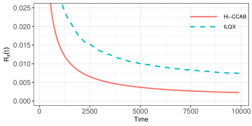
Figure 1: Time-averaged regret for Hi-CCAB and the iterated Lasso-regularized quasi-likelihood regression (ILQX) proposed by Ban and Keskin, (2021).

We follow the simulation set-up introduced by Ban and Keskin, (2021): in particular, generate demands and rewards according to the model (7)–(8), with parameter vectors

$$\alpha$$

$$\beta$$

and the variable $\epsilon_{t}$ follows a normal distribution with mean zero and standard deviation $0.01$.

We compare the time-averaged regret $\mathcal{R}^{\pi}(t)$ of ILQX (iterated lasso-regularized quasi-likelihood regression with price experimentation) proposed by Ban and Keskin, (2021) with Hi-CCAB. The basic idea of ILQX is to use LASSO to estimate the unknown $\alpha$ and $\beta$, and at the same time to conduct price experiments for at least an order of $\sqrt{t}$ times. As shown in Section 2.5.2, their revenue model (8) is a special case of our model (2).

Figure 1 compares the performance, measured by the time-averaged regret, of Hi-CCAB and ILQX. It is clear that Hi-CCAB converges faster than ILQX. As shown in Ban and Keskin, (2021), ILQX converges faster than the greedy iterated least squares (Keskin and Zeevi, 2014, Qiang and Bayati, 2016), which decides the price based on the least square estimate of the unknown $\alpha$ and $\beta$ at each iteration without experiments. We see that Hi-CCAB has better performance than various dynamic pricing algorithms, and is competitive in a continuum armed bandit problem.

5.2 Simulation Experiment II: Bandit Models

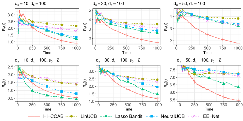
Figure 2: Time-averaged regret in a multi-armed linear bandit setup for Hi-CCAB and other bandit algorithms. The upper row corresponds to a non-sparse case and the lower one corresponds to a sparse case.

In this simulation study, we consider a multi-armed linear bandit, which (as discussed previously) corresponds to a special case of our model with ${\bm{\Theta}}^{*}=({\bm{\beta}}_{1},{\bm{\beta}}_{2},\cdots,{\bm{\beta}}_{m})^{\top}$. In particular, each row of ${\bm{\Theta}}^{*}$ is the parameter of each arm for the multi-arm contextual bandit. Specifically, we set the number of arms $d_{a}=\{10,30,50\}$ and the dimension of covariates $d_{x}=100$. For the representation matrix ${\bm{\Theta}}^{*}$, we consider both non-sparse and sparse cases. For the non-sparse case, we generate ${\bm{\Theta}}^{*}={\bm{U}}{\bm{D}}{\bm{V}}^{\top}$ where ${\bm{U}}\in\mathbb{R}^{d_{a}\times r},{\bm{V}}\in\mathbb{R}^{d_{x}\times r}$ ($r=5$), and ${\bm{D}}$ is a diagonal matrix with $(1,0.9,0.9,0.8,0.5)$ as the diagonal entries. All entries of ${\bm{U}}$ and ${\bm{V}}$ are first generated from i.i.d. $N(0,1)$, and then applied Gram–Schmidt to make each column orthogonal. The matrix ${\bm{U}}$ is scaled to have $\ell_{2}$-norm $\sqrt{d_{a}}$ for each column so that the rewards are comparable across different $d_{a}$’s. For the sparse case, each row of ${\bm{\Theta}}^{*}$ is set as zero except for $s_{0}=2$ randomly selected elements that are drawn from $N(0,1)$. We generate the covariate ${\bm{x}}\overset{i.i.d}{\sim}N(0,{\bm{I}}_{d_{x}})$ and the rewards from our model (3) with variance of the reward error (20) $\sigma^{2}=0.01$.

We compare Hi-CCAB against a) the LinUCB (Li et al., 2010), which is an extension of the traditional Upper Confidence Bound (UCB) algorithm to the contextual multi-armed bandit settings; b) a Lasso Bandit for high-dimensional contextual bandits (Bastani and Bayati, 2020); c) NeuralUCB, a neural-network-based method for contextual bandits (Zhou et al., 2020) and d) EE-Net (Ban et al., 2022), which uses two separate neural networks for exploration and exploitation. Details of the tuning parameters of each algorithm are provided in Appendix 9.1.

Figure 2 shows the regret averaged over 50 simulations. For the non-sparse case in the upper row, Hi-CCAB converges faster than all other methods. The advantage of Hi-CCAB is more pronounced when the dimension of arms becomes larger. This phenomenon demonstrates the advantages of leveraging the low-rank structure, especially when the dimension is high. It is expected that when the dimensions of the action and covariates continue to grow, the gap between Hi-CCAB and the alternatives will further enlarge. For the sparse case in the lower row—a setting not to the advantage of Hi-CCAB—when the dimension of arms is relatively small ($d_{a}=10$), Lasso Bandit converges faster but the margin between Hi-CCAB and Lasso Bandit is small. As the number of arms increases, Hi-CCAB outperforms all other methods. This phenomenon comes as a surprise since in this sparse setup, the matrix ${\bm{\Theta}}^{*}$ is close to full rank. This surprising result may be explained as follows. As the number of arms increases, we observe that the top singular vectors explain most variability and thus approximate ${\bm{\Theta}}^{*}$ well enough. In particular, when $d_{a}=10$, the top 20% singular vectors account for around 40% of the variance, while when $d_{a}=50$, they account for almost 60%. For the top 50% singular vectors, the percentage of variance explained is around 70% when $d_{a}=10$, while it is almost 90% when $d_{a}=50$. In addition, Hi-CCAB is adaptive since it does not require prior knowledge on the rank of ${\bm{\Theta}}^{*}$ and it penalizes more when $t$ is small and the penalization gradually decreases as $t$ increases. In sum, our penalized estimator is robust for such sparse settings, especially for high dimensional settings.

5.3 Case Study I: Instant Noodle Company

In this section, we revisit the instant noodle case study first introduced in Section 2.1. We begin with a more detailed descriptions of the data and experiment setup and results. Our method can provide assortment and pricing decisions simultaneously, which increases the cumulative sales by a factor of $4$ times, and provide insightful interpretations of customer behavior through the latent factors of the estimated representation matrix $\widehat{{\bm{\Theta}}}$.

Data Description.

The original data contains daily sales of $N=176$ products (SKUs) across $369$ cities over the time period from March 1st, 2021 to May 31st, 2022, for a total of $T=456$ days. The sales are split across 31 Chinese provinces. Each product consists of either a single flavor of noodles (13 possible choices), or an assortment of flavors with varying counts/flavor. The assortment and price of each product change daily. The assortment and prices were the same across locations. The maximum number of products to be shown on the homepage is $K=30$. Thus, the total possible of combinations is ${N\choose K}={176\choose 30}$; if each such combination is associated with an action, the action space is extremely high-dimensional, and standard multi-arm bandit algorithms are computationally prohibitive.

Experiment Setup and Results.

To apply Hi-CCAB, we specify the action vectors ${\bm{a}}_{t}$ and the covariate vectors $\{{\bm{x}}_{t,\ell}\}_{\ell=1}^{L}$ with $L=31$ at given time $t$ following the setup in Section 2.1. The action vector takes the form

$${\bm{a}}=({\bm{f}}_{1},{\bm{f}}_{1}^{2},p_{1},p_{1}^{2},\cdots,{\bm{f}}_{K},{\bm{f}}_{K}^{2},p_{K},p_{K}^{2},1)\in{}^{2(m+1)K+1=841},$$

where ${\bm{f}}_{k}=(f_{k,1},\cdots,f_{k,m})$ is a vector of non-negative integers to denote the counts of $m=13$ flavors, $p_{k}$ is the price, and ${\bm{f}}_{k}^{2}$ denotes the vector formed by squaring each component of ${\bm{f}}_{k}$. The context vector ${\bm{x}}_{\ell}\in\mathbb{R}^{50}$ for location $\ell$ includes dummy variables of 31 provinces, the year 2021/2022, 12 months, weekdays, and an indicator of the annual sales event on Jun 18 and Nov 11. See Appendix 9.2 for complete details.

In order to run simulations using the dataset, we first create a pseudo-ground-truth model by estimating ${\bm{\Theta}}^{*}$ and the variance of the reward error $\sigma^{2}$ as in equation (20) using the full dataset. The pair $({\bm{\Theta}}^{*},\sigma)$ define what we refer to as the pseudo-ground-truth for the problem.

Using this fitted model, we assess the validity of bilinear reward assumption (3) via out-of-sample sales prediction. In particular, we do so via a leave-one-out (LOO) approach: recursively over the index $i$, we compute an estimate $\widehat{{\bm{\Theta}}}$ of the true representation matrix with the $i^{th}$ sample removed, and then use this fit to predict the $i^{th}$ reward. We then measure the performance of these LOO predictions relative to the actual rewards; doing so yields an out-of-sample prediction error rate of approximately 7%. See Appendix 9.2 for details.

Initializing Hi-CCAB with the initial step number $t_{\mathchoice{\raisebox{0.0pt}{\leavevmode\resizebox{10.00948pt}{4.0pt}{\hbox{\raisebox{0.0pt}{$\displaystyle init$}}}}}{\raisebox{0.0pt}{\leavevmode\resizebox{10.00948pt}{4.0pt}{\hbox{\raisebox{0.0pt}{$\textstyle init$}}}}}{\raisebox{0.0pt}{\leavevmode\resizebox{10.00948pt}{4.0pt}{\hbox{\raisebox{0.0pt}{$\scriptstyle init$}}}}}{\raisebox{0.0pt}{\leavevmode\resizebox{10.00945pt}{4.0pt}{\hbox{\raisebox{0.0pt}{$\scriptscriptstyle init$}}}}}}=100$ and $\lambda_{0}$ according to Algorithm 1, we then run $100$ trials, in each of which we iterate from $t_{\mathchoice{\raisebox{0.0pt}{\leavevmode\resizebox{10.00948pt}{4.0pt}{\hbox{\raisebox{0.0pt}{$\displaystyle init$}}}}}{\raisebox{0.0pt}{\leavevmode\resizebox{10.00948pt}{4.0pt}{\hbox{\raisebox{0.0pt}{$\textstyle init$}}}}}{\raisebox{0.0pt}{\leavevmode\resizebox{10.00948pt}{4.0pt}{\hbox{\raisebox{0.0pt}{$\scriptstyle init$}}}}}{\raisebox{0.0pt}{\leavevmode\resizebox{10.00945pt}{4.0pt}{\hbox{\raisebox{0.0pt}{$\scriptscriptstyle init$}}}}}}=100$ to $T=456$. At each iteration $t$, we first estimate $\widehat{\bm{\Theta}}_{t}$ and make an assortment-pricing decision ${\bm{a}}_{t+1}$ that maximizes the total sales given the covariate ${\bm{x}}_{t+1}$ according to Algorithm 1, and then generate a reward based on the pseudo-ground-truth model with $({\bm{\Theta}}^{*},\sigma)$.

We evaluate the performance of Hi-CCAB in terms of the time-averaged regret (5) and the percentage gain of the cumulative sales by comparing with the original actions, since no existing bandit algorithms are applicable to this joint assortment-pricing problem with contextual information.

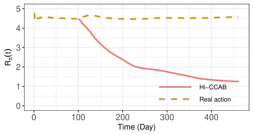
(a) Time-averaged regret (in 1 million RMB).

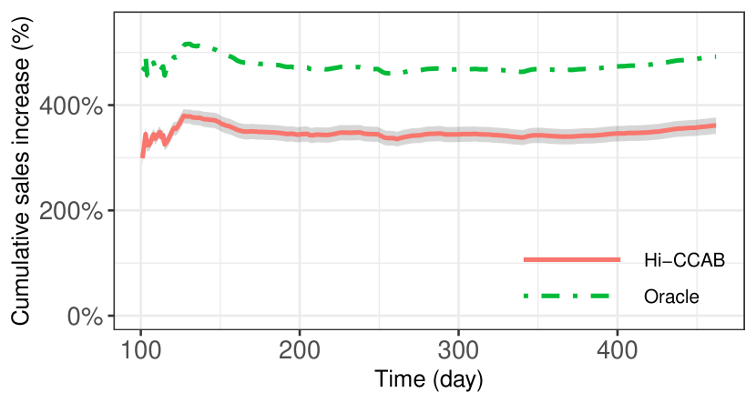
(b) Percentage cumulative sales gain.

Figure 3: Performance of Hi-CCAB compared with real actions in terms of the time-averaged regret and the percentage cumulative gain in revenue. The boundaries of the shadow are the 5th and 95th quantiles.

Figure 3(a) shows the time-averaged regret and Figure 3(b) shows the percentage gain in cumulative sales compared to the real sales (averaged over 100 simulations). The expected average regret of Hi-CCAB converges to zero while that of original actions remains flat. In terms of percentage gain in cumulative sales, Hi-CCAB boosts cumulative sales by almost 4 times. The cumulative sales by Hi-CCAB is also converging to the clairvoyant sales obtained by the oracle solution.

Interpretation of the Representation Matrix ${\bm{\Theta}}^{*}$.

One advantage of our model is the interpretability which allows us to gain insights from the representation matrix ${\bm{\Theta}}^{*}$. Specifically, our model is able to discover the underlying factors of the effect of arm-covariate pairs on the reward. In the following, we examine the pseudo ground truth ${\bm{\Theta}}^{*}$ we obtained using all the data.

The rank of ${\bm{\Theta}}^{*}$ is 4 with the singular values being $(1.9,0.2,0.02,0.00003)$. The leading singular value dominates the rest and thus the leading singular vectors are the most important ones in explaining the effect on the reward, which we will focus on in what follows.

Figure 4 shows the loadings for different covariates (i.e., the leading right singular vector) and our algorithm is able to learn interpretable patterns of the effects on the reward – for weekdays, the effects are drastically different during the weekend and during the weekend; for months, the effects show different patterns during the promotion month (June and November) from other months; for location, the effects of the coastal provinces are different from the rest, which exactly corresponds to the levels of economic development of different regions in China. In sum, our model can exploit the underlying structure of the covariates and provide insights into purchasing behavior and seasonality.

On the other hand, Table 1 explores the (scaled) loadings for the arm on May 29th 2022, the last Sunday in our data (i.e., the leading left singular vectors multiplied with $\left\langle{\bm{v}}_{1},\,\bar{{\bm{x}}}\right\rangle$ where $\bar{{\bm{x}}}$ is the average of ${\bm{x}}_{\ell}$ for $\ell=1,\ldots,L$ on May 29th 2022). Specifically, we investigate the effect of flavors on the reward given the context. We take the average of the loadings of the linear and quadratic terms for each flavor in all 30 products and compare with the total sales of each flavor across all Sundays in the months of May. For ease of comparison, we further scale the sales and the loadings by their corresponding largest numbers. The loadings and sales are closely related to each other. As in Table 1, on May 29th 2022, flavor $1$ (denoted $F1$) has the largest effect, followed by flavors $13$, $10$, $11$, $7$, and $9$. Therefore, our model learns the values of the flavors (per unit).

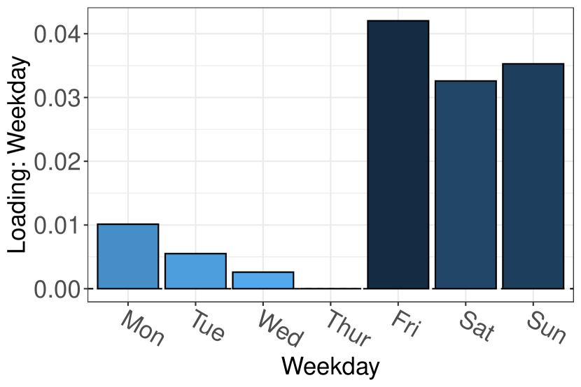
(a) Weekday

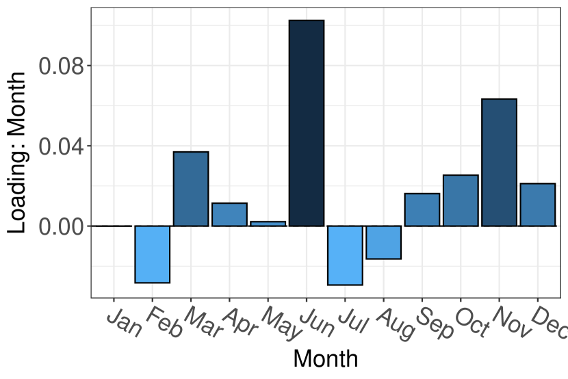
(b) Month

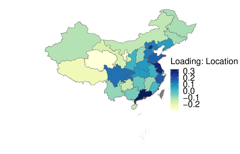
(c) Location

Figure 4: Loadings of the leading right singular vectors for the covariates.

	F1	F2	F3	F4	F5	F6	F7	F8	F9	F10	F11	F12	F13
Sales	1.00	0.05	0.00	0.00	0.00	0.03	0.19	0.00	0.08	0.19	0.18	0.00	0.38
$\tilde{u}_{1}$ (linear)	1.00	0.11	0.00	0.00	0.00	0.05	0.23	0.01	0.13	0.50	0.25	0.03	0.51
$\tilde{u}_{1}$ (quadratic)	1.00	0.07	0.00	0.00	0.00	0.03	0.17	0.01	0.09	0.41	0.19	0.02	0.42

Table 1: Total sales and loadings of the linear and quadratic terms (scaled) of the 13 flavors.

Limitations.

We would like to point out that the increase in cumulative sales in real life could be less than four times as claimed because there will be additional constraints on the action space due to constraints on production or supply chain.

5.4 Case Study II: Manicure Start-up

In this section, we apply our model to a joint assortment-pricing problem faced by a manicure start-up. Unlike the noodle company treated in Section 5.3, this start-up company updates its product line quite frequently, and is interested in determining the color and style to guide its designs as well as optimal ways to offer discounts and promotions. Accordingly, we formulate the problem differently by using the aggregated product features and discount rate as the action vector, thereby demonstrating the flexibility of our model. As we discuss here, our method not only boosts profit, but also provides insightful interpretations.

Data Description.

The start-up provided transaction-level data over the period February 1st, 2020 to April 26th, 2021, for a total of $T=451$ days. Over this period, the product line was updated on a regular basis, with a maximum number of products available online being 74 during October 2020, and a total of 84 products (SKU) avaiable at some point during the entire time horizon. Each product can be described by its texture (glossy versus matted), transparency, and colors (solid or multiple colors). The store also collaborates with designers and we measure their popularity by the number of their Instagram followers. The price of the products is fixed for designer vs non-designer and the cost of each product is known. Being a start-up company in a growth phase, they provide discount promotions on a regular basis to attract more customers. For each transaction, the data contains the purchased product, total price, discount, shipping address, and an indicator of accepting marketing or not.

Experiment Setup and Results.

Instead of a specific assortment of manicures, the start-up is most interested in the trend of colors and styles. At the same time, they need to decide on the number of available products and designer products as well as promotions on a daily basis. Therefore, we use the daily aggregated product information as the action vector and the daily aggregated customer information as well as the time as the covariates. Specifically, we specify the action vectors ${\bm{a}}$ as the count of different colors used in all the manicures (black, white, gray, red, orange, yellow, green, blue, indigo, and violet), styles (the proportions of glossy, transparent and designer manicures, and the total number of Instagram followers of the designers), the discount rate as well as the quadratic terms of all the above, leading to $d_{a}=31$. The covariate vector ${\bm{x}}$ includes location (percentages of purchase from Midwest, Northeast, South, and West), demographic proxies (average of median income and racial distribution by ZIP code), and the proportions of customers accepting marketing of last period, along with dummy variables for the 12 months, weekdays and public holidays. The dimension of the covariate vector is $d_{x}=30$. Given that costs are known, we use profit rather than total sales revenue as our reward $y$.

Similar to our case study described in Section 5.3, we first create a pseudo-truth model by estimating ${\bm{\Theta}}^{*}$ and $\sigma$ using all data and check our model assumptions in Appendix 9.3. We then run the simulation a total of $100$ times with initialization $t_{\mathchoice{\raisebox{0.0pt}{\leavevmode\resizebox{10.00948pt}{4.0pt}{\hbox{\raisebox{0.0pt}{$\displaystyle init$}}}}}{\raisebox{0.0pt}{\leavevmode\resizebox{10.00948pt}{4.0pt}{\hbox{\raisebox{0.0pt}{$\textstyle init$}}}}}{\raisebox{0.0pt}{\leavevmode\resizebox{10.00948pt}{4.0pt}{\hbox{\raisebox{0.0pt}{$\scriptstyle init$}}}}}{\raisebox{0.0pt}{\leavevmode\resizebox{10.00945pt}{4.0pt}{\hbox{\raisebox{0.0pt}{$\scriptscriptstyle init$}}}}}}=100$.

Figure 5 shows the performance of Hi-CCAB in terms of the time-averaged regret and percentage cumulative gain in profit compared to the real actions (averaged over 100 simulations). The finding is similar to those from Section 5.3: in particular, the time-averaged regret of Hi-CCAB converges to zero, whereas the same quantity associated with the original choice of actions stays bounded away from zero. Meanwhile, the Hi-CCAB approach boosts the cumulative profit by more than $7$ times.

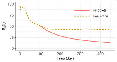
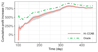
(a) Time-averaged regret (in 1 thousand USD)		(b) Percentage cumulative profit gain

Figure 5: Performance of Hi-CCAB compared with real actions in terms of the time-averaged regret and the percentage cumulative gain in profit. The boundaries of the shadow are the $5^{th}$ and $95^{th}$ quantiles.

Interpretation of the Representation Matrix.

Our procedure learns a representation matrix $\widehat{{\bm{\Theta}}}$, and its singular value decomposition has interesting structure. It has rank $5$, which is low compared to its dimensions $31$ by $30$.

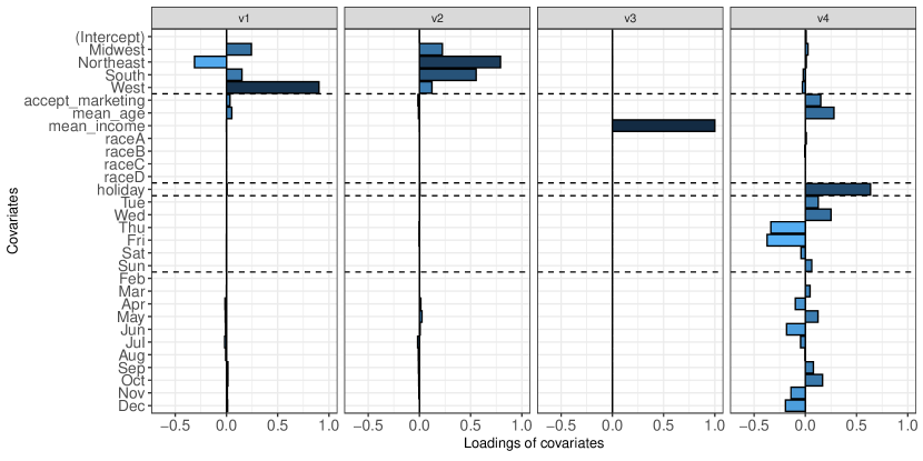
Figure 6: Loadings associated with context vectors, as illustrated by stem plots of the singular vectors ${\bm{v}}_{1}$, ${\bm{v}}_{2}$, ${\bm{v}}_{3}$ and ${\bm{v}}_{4}$. Dashed lines separate the covarites into locations, customers demographic proxies, a holiday indicator, weekdays, and months.

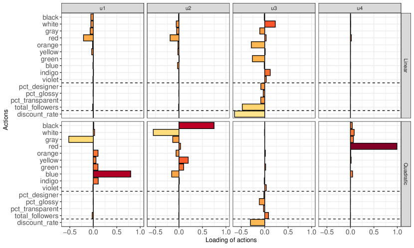
Figure 7: Loadings associated with the action vectors, as illustrated by stem plots of the left singular vectors ${\bm{u}}_{1}$, ${\bm{u}}_{2}$, ${\bm{u}}_{3}$, and ${\bm{u}}_{4}$. Dashed lines separate the actions into colors, styles, and discount rate.

Its ordered singular values are given by $(0.66,0.54,0.22,0.16,0.0008)$. Noting that the last singular value is negligible compared to the first four, we focus our discussion on the singular vectors associated with the first four singular values.

Figures 6 and 7 illustrate (respectively) the loadings of the covariates and actions. At a high level, the four factors capture the Western market $({\bm{u}}_{1},{\bm{v}}_{1})$, Northeastern/Southern market $({\bm{u}}_{2},{\bm{v}}_{2})$, income effect $({\bm{u}}_{3},{\bm{v}}_{3})$, and time effect $({\bm{u}}_{4},{\bm{v}}_{4})$ respectively. The covariate loadings associated with the factors are well-separated, which facilitates interpretations for the actions. Let us first look at color and style. For color, we examine the quadratic terms since the color action vector represents the absolute count of each color’s appearance in the manicures so that the quadratic terms dominate. Comparing the Western market (${\bm{u}}_{1}$ and ${\bm{v}}_{1}$) and Northeastern/Southern market (${\bm{u}}_{2}$ and ${\bm{v}}_{2}$), we observe distinct geographical preferences in color choices—blue is more popular in the Western market while black is preferred in the Northeastern/Southern market; gray does not sell well in the west while white is lackluster in the Northeast and South. As for the income factor (${\bm{u}}_{3},{\bm{v}}_{3}$), the color preferences are reflected in the linear terms (since the quadratic terms are negligible) where white and indigo are more sought-after among higher-income customers while gray, orange, and green are less favorable. For the time factor $({\bm{u}}_{4},{\bm{v}}_{4})$, red stands out as a festive favorite, aligning with holiday trends. In terms of style, their loadings concentrate in the income factor $({\bm{u}}_{3},{\bm{v}}_{3})$. Customers with higher incomes show less interest in designer and glossy products and care less about the popularity of the designers.

Next, we investigate the effects of discounts. Loadings of discount rate are concentrated in the vector ${\bm{u}}_{3}$, associated with the income factor tracked by the pair (${\bm{u}}_{3},{\bm{v}}_{3}$). Generally, for high-income customers, higher discount rates yield lower profits. One plausible explanation goes as follows: the demand function (7) is controlled by the market size (via the linear term) and the price sensitivity (via the quadratic term), both of which depend on income. In our case, the market size in the linear term dominates due to relatively small discount rates (median: $0.067$; 5th and 95th quantiles: $0.03$ and $0.18$) and the fact that the linear term in ${\bm{u}}_{3}$ outweighs the quadratic term. Therefore, the negative linear term suggests that profits will be lower with higher discount rates for our customer base whose household income is of mid-to-high levels (ranging from 95K to 110K).

As income increases, so does the market size, particularly for hedonic purchases such as manicures among our customer base. Consequently, discounts would have incurred more profit loss for higher-income customers. On the other hand, it is crucial to note that as a start-up, customer expansion and retention are vital for long-term growth, in which context discounts can serve as effective incentives. This unique additional dynamics of a startup, however, can only be revealed by a longer sequence of data. That being said, this longer-term aspect of decision-making, while beyond the scope of our current case study, is worthy of further investigation.

6 Conclusions and Future Directions

The growing need for online and data-driven decision-making has led to increased interested in bandit models among both theorists and practitioners. Nonetheless, at least to date, we are not aware of any work on contextual bandits in which both the covariate and action spaces are high-dimensional. Our work in this paper is motivated by applications of bandits—among them the joint assortment-pricing problem—that have this “doubly” high-dimensional nature. We proposed a structured bilinear matrix model for capturing interactions between covariates and actions in determing the reward function. This model is reasonably general, including a number of structured bandit and pricing models as special cases; at the same time, it is also highly interpretable in that the spectral structure of representation matrix captures interactions between actions and contexts.

We proposed an efficient algorithm Hi-CCAB that interleaves steps of low-rank matrix estimation with exploration/exploitation, and we proved a non-asymptotic upper bound on its time-averaged regret. In addition, the generality and flexibility of our model enable its application to the joint assortment-pricing problem, each of which has been studied extensively in operations research and marketing but not jointly. In real case studies with the largest instant noodle producers and a manicure start-up, our method can boost sales/profits, while also provide insights into the underlying structure of the effect on the reward of arms and covariates such as purchasing behaviors.

We conclude by discussing some future research directions. One key contribution of this paper is our novel model for doubly high-dimensional contextual bandits and its application to the joint assortment-pricing problem. We provided a non-asymptotic upper bound on the regret while future work could aim to improve this regret analysis by tightening the regret bound given the outstanding performance of Hi-CCAB compared to other bandit algorithms, and establishing a potentially matching lower bound. Another direction is on its generality in terms of mathematical expressiveness, i.e., when the choice of covariate vector and action vector are particular feature maps as explained in Appendix 7, with a particular focus on theory.

In terms of applications, the flexibility of model allows for applications to other multiple decision-making problems in diverse sectors, such as other business settings and healthcare. In the realm of business, our model can incorporate other quantifiable actions for joint decision-making, particularly in marketing and operations. Furthermore, it offers flexibility in the objective, allowing it to be tailored to suit different outcomes, such as social benefits for social enterprises and the Environmental, Social, and Governance (ESG) performance for responsible investment. In healthcare, especially personalized healthcare, our model holds high potential. For instance, health monitoring, which provides action suggestions based on individual health conditions, aligns with our model. Actions like sleeping patterns, exercise regimens, social media usage, and dietary choices can be considered in high-dimensional and continuous arms. Meanwhile, health outcome also depends on contextual variables such as age, gender, weight, height, basic health status, and compliance level. Traditional bandit models do not suffice for such doubly high-dimensional contextual settings, but our bilinear model with a low-rank ${\bm{\Theta}}^{*}$ for mean reward fits well, as health effects of actions and user characteristics can typically be captured by a few latent factors.

Assessing the performance of our algorithms in other applications, particularly within the field of personalized healthcare, would be practically valuable. Finally, our case studies partially relied on simulations to evaluate the efficacy of our method; however, real operational settings often impose additional constraints on the action space. In order to gauge and improve the real-world performance of our methods, we anticipate further collaboration with companies in carrying out live deployments.

Supplementary material

7 Nonlinear Relationship Representations and Extensions to Reproducing Kernel Hilbert Spaces

In this section, we describe how our bilinear form can capture complicated non-linear effects in the actions and covariates. Suppose that the original (primitive) action vector is given by $\bm{a}_{\mathchoice{\raisebox{0.0pt}{\leavevmode\resizebox{10.8987pt}{4.0pt}{\hbox{\raisebox{0.0pt}{$\displaystyle base$}}}}}{\raisebox{0.0pt}{\leavevmode\resizebox{10.8987pt}{4.0pt}{\hbox{\raisebox{0.0pt}{$\textstyle base$}}}}}{\raisebox{0.0pt}{\leavevmode\resizebox{10.89868pt}{4.0pt}{\hbox{\raisebox{0.0pt}{$\scriptstyle base$}}}}}{\raisebox{0.0pt}{\leavevmode\resizebox{10.8987pt}{4.0pt}{\hbox{\raisebox{0.0pt}{$\scriptscriptstyle base$}}}}}}=(a_{1},a_{2},\ldots,a_{d_{1}})\in{}^{d_{1}}$. We then define an augmented action vector by including all polynomial terms of $\bm{a}_{\mathchoice{\raisebox{0.0pt}{\leavevmode\resizebox{10.8987pt}{4.0pt}{\hbox{\raisebox{0.0pt}{$\displaystyle base$}}}}}{\raisebox{0.0pt}{\leavevmode\resizebox{10.8987pt}{4.0pt}{\hbox{\raisebox{0.0pt}{$\textstyle base$}}}}}{\raisebox{0.0pt}{\leavevmode\resizebox{10.89868pt}{4.0pt}{\hbox{\raisebox{0.0pt}{$\scriptstyle base$}}}}}{\raisebox{0.0pt}{\leavevmode\resizebox{10.8987pt}{4.0pt}{\hbox{\raisebox{0.0pt}{$\scriptscriptstyle base$}}}}}}$ up to order $N_{1}$—that is

$${\bm{a}}\defn(1,a_{1},a_{2},\ldots,a_{d_{1}},a_{1}^{2},a_{2}^{2},\ldots,a_{d_{1}}^{2},a_{1}a_{2},a_{1}a_{3},\ldots,a_{1}a_{d_{1}},a_{2}a_{3},\ldots,a_{2}a_{d_{1}},\ldots,a_{d_{1}-1}a_{d_{1}},\ldots\\ \ldots,a_{1}^{N_{1}},\cdots,a_{d_{1}}^{N_{1}},a_{1}^{N_{1}-1}a_{2},a_{1}^{N_{1}-1}a_{3},\ldots,a_{1}^{N_{1}-1}a_{d_{1}},\ldots,a_{d_{1}}^{N_{1}-1}a_{d_{1}-1},\ldots,a_{d_{1}-N_{1}+1}a_{d_{1}-N_{1}+2}\cdots a_{d_{1}}).$$ (21)

Similarly, let $\bm{x}_{\mathchoice{\raisebox{0.0pt}{\leavevmode\resizebox{10.8987pt}{4.0pt}{\hbox{\raisebox{0.0pt}{$\displaystyle base$}}}}}{\raisebox{0.0pt}{\leavevmode\resizebox{10.8987pt}{4.0pt}{\hbox{\raisebox{0.0pt}{$\textstyle base$}}}}}{\raisebox{0.0pt}{\leavevmode\resizebox{10.89868pt}{4.0pt}{\hbox{\raisebox{0.0pt}{$\scriptstyle base$}}}}}{\raisebox{0.0pt}{\leavevmode\resizebox{10.8987pt}{4.0pt}{\hbox{\raisebox{0.0pt}{$\scriptscriptstyle base$}}}}}}\in{}^{d_{2}}$ denote the original (primitive) context vector. We then define an extended context vector ${\bm{x}}$ by including all the polynomial terms of $\bm{x}_{\mathchoice{\raisebox{0.0pt}{\leavevmode\resizebox{10.8987pt}{4.0pt}{\hbox{\raisebox{0.0pt}{$\displaystyle base$}}}}}{\raisebox{0.0pt}{\leavevmode\resizebox{10.8987pt}{4.0pt}{\hbox{\raisebox{0.0pt}{$\textstyle base$}}}}}{\raisebox{0.0pt}{\leavevmode\resizebox{10.89868pt}{4.0pt}{\hbox{\raisebox{0.0pt}{$\scriptstyle base$}}}}}{\raisebox{0.0pt}{\leavevmode\resizebox{10.8987pt}{4.0pt}{\hbox{\raisebox{0.0pt}{$\scriptscriptstyle base$}}}}}}$ up to order $N_{2}$.

With these definitions, the expected reward takes the form

$${\bm{a}}^{\top}{\bm{\Theta}}{\bm{x}}=\sum_{\begin{subarray}{c}k_{i},\ell_{j}\geq 0\\ k_{1}+k_{2}+\ldots+k_{d_{1}}\leq N_{1},\\ \ell_{1}+\ell_{2}+\ldots+\ell_{d_{2}}\leq N_{2}\end{subarray}}h(k_{1},k_{2},\ldots,k_{N_{1}},\ldots,\ell_{1},\ell_{2},\ldots,\ell_{N_{2}})\cdot a_{1}^{k_{1}}a_{2}^{k_{2}}\cdots a_{d_{1}}^{k_{d_{1}}}\cdot x_{1}^{\ell_{1}}x_{2}^{\ell_{2}}\cdots x_{d_{2}}^{\ell_{d_{2}}},$$ (22)

where $h(k_{1},k_{2},\ldots,k_{N_{1}},\ldots,\ell_{1},\ell_{2},\ldots,\ell_{N_{2}})$ is an element in ${\bm{\Theta}}$.

It is evident that the function $g(\bm{a}_{\mathchoice{\raisebox{0.0pt}{\leavevmode\resizebox{10.8987pt}{4.0pt}{\hbox{\raisebox{0.0pt}{$\displaystyle base$}}}}}{\raisebox{0.0pt}{\leavevmode\resizebox{10.8987pt}{4.0pt}{\hbox{\raisebox{0.0pt}{$\textstyle base$}}}}}{\raisebox{0.0pt}{\leavevmode\resizebox{10.89868pt}{4.0pt}{\hbox{\raisebox{0.0pt}{$\scriptstyle base$}}}}}{\raisebox{0.0pt}{\leavevmode\resizebox{10.8987pt}{4.0pt}{\hbox{\raisebox{0.0pt}{$\scriptscriptstyle base$}}}}}},\bm{x}_{\mathchoice{\raisebox{0.0pt}{\leavevmode\resizebox{10.8987pt}{4.0pt}{\hbox{\raisebox{0.0pt}{$\displaystyle base$}}}}}{\raisebox{0.0pt}{\leavevmode\resizebox{10.8987pt}{4.0pt}{\hbox{\raisebox{0.0pt}{$\textstyle base$}}}}}{\raisebox{0.0pt}{\leavevmode\resizebox{10.89868pt}{4.0pt}{\hbox{\raisebox{0.0pt}{$\scriptstyle base$}}}}}{\raisebox{0.0pt}{\leavevmode\resizebox{10.8987pt}{4.0pt}{\hbox{\raisebox{0.0pt}{$\scriptscriptstyle base$}}}}}})={\bm{a}}^{\top}{\bm{\Theta}}{\bm{x}}$ as in Equation 22 can capture nonlinear relationships in terms of $(\bm{a}_{\mathchoice{\raisebox{0.0pt}{\leavevmode\resizebox{10.8987pt}{4.0pt}{\hbox{\raisebox{0.0pt}{$\displaystyle base$}}}}}{\raisebox{0.0pt}{\leavevmode\resizebox{10.8987pt}{4.0pt}{\hbox{\raisebox{0.0pt}{$\textstyle base$}}}}}{\raisebox{0.0pt}{\leavevmode\resizebox{10.89868pt}{4.0pt}{\hbox{\raisebox{0.0pt}{$\scriptstyle base$}}}}}{\raisebox{0.0pt}{\leavevmode\resizebox{10.8987pt}{4.0pt}{\hbox{\raisebox{0.0pt}{$\scriptscriptstyle base$}}}}}},\bm{x}_{\mathchoice{\raisebox{0.0pt}{\leavevmode\resizebox{10.8987pt}{4.0pt}{\hbox{\raisebox{0.0pt}{$\displaystyle base$}}}}}{\raisebox{0.0pt}{\leavevmode\resizebox{10.8987pt}{4.0pt}{\hbox{\raisebox{0.0pt}{$\textstyle base$}}}}}{\raisebox{0.0pt}{\leavevmode\resizebox{10.89868pt}{4.0pt}{\hbox{\raisebox{0.0pt}{$\scriptstyle base$}}}}}{\raisebox{0.0pt}{\leavevmode\resizebox{10.8987pt}{4.0pt}{\hbox{\raisebox{0.0pt}{$\scriptscriptstyle base$}}}}}})$. Furthermore, by suitably choosing the orders $(N_{1},N_{2})$ of lifting, such a function $g$ can be used to approximate any continuous functions $(\bm{a}_{\mathchoice{\raisebox{0.0pt}{\leavevmode\resizebox{10.8987pt}{4.0pt}{\hbox{\raisebox{0.0pt}{$\displaystyle base$}}}}}{\raisebox{0.0pt}{\leavevmode\resizebox{10.8987pt}{4.0pt}{\hbox{\raisebox{0.0pt}{$\textstyle base$}}}}}{\raisebox{0.0pt}{\leavevmode\resizebox{10.89868pt}{4.0pt}{\hbox{\raisebox{0.0pt}{$\scriptstyle base$}}}}}{\raisebox{0.0pt}{\leavevmode\resizebox{10.8987pt}{4.0pt}{\hbox{\raisebox{0.0pt}{$\scriptscriptstyle base$}}}}}},\bm{x}_{\mathchoice{\raisebox{0.0pt}{\leavevmode\resizebox{10.8987pt}{4.0pt}{\hbox{\raisebox{0.0pt}{$\displaystyle base$}}}}}{\raisebox{0.0pt}{\leavevmode\resizebox{10.8987pt}{4.0pt}{\hbox{\raisebox{0.0pt}{$\textstyle base$}}}}}{\raisebox{0.0pt}{\leavevmode\resizebox{10.89868pt}{4.0pt}{\hbox{\raisebox{0.0pt}{$\scriptstyle base$}}}}}{\raisebox{0.0pt}{\leavevmode\resizebox{10.8987pt}{4.0pt}{\hbox{\raisebox{0.0pt}{$\scriptscriptstyle base$}}}}}})\mapsto f(\bm{a}_{\mathchoice{\raisebox{0.0pt}{\leavevmode\resizebox{10.8987pt}{4.0pt}{\hbox{\raisebox{0.0pt}{$\displaystyle base$}}}}}{\raisebox{0.0pt}{\leavevmode\resizebox{10.8987pt}{4.0pt}{\hbox{\raisebox{0.0pt}{$\textstyle base$}}}}}{\raisebox{0.0pt}{\leavevmode\resizebox{10.89868pt}{4.0pt}{\hbox{\raisebox{0.0pt}{$\scriptstyle base$}}}}}{\raisebox{0.0pt}{\leavevmode\resizebox{10.8987pt}{4.0pt}{\hbox{\raisebox{0.0pt}{$\scriptscriptstyle base$}}}}}},\bm{x}_{\mathchoice{\raisebox{0.0pt}{\leavevmode\resizebox{10.8987pt}{4.0pt}{\hbox{\raisebox{0.0pt}{$\displaystyle base$}}}}}{\raisebox{0.0pt}{\leavevmode\resizebox{10.8987pt}{4.0pt}{\hbox{\raisebox{0.0pt}{$\textstyle base$}}}}}{\raisebox{0.0pt}{\leavevmode\resizebox{10.89868pt}{4.0pt}{\hbox{\raisebox{0.0pt}{$\scriptstyle base$}}}}}{\raisebox{0.0pt}{\leavevmode\resizebox{10.8987pt}{4.0pt}{\hbox{\raisebox{0.0pt}{$\scriptscriptstyle base$}}}}}})$ to arbitrary accuracy on any compact set $\mathcal{C}$. (E.g., see the paper Foupouagnigni and Mouafo Wouodjié, (2020) for results on the approximation (multivariate) functions with Bernstein polynomials). Note that besides polynomial type basis (21) that yields the form (22), we can also use other bases such as Fourier or Haar.

Sometimes we may want to use the basis in an RKHS defined with kernel $\mathscr{K}_{\bm{x}_{\mathchoice{\raisebox{0.0pt}{\leavevmode\resizebox{10.8987pt}{4.0pt}{\hbox{\raisebox{0.0pt}{$\displaystyle base$}}}}}{\raisebox{0.0pt}{\leavevmode\resizebox{10.8987pt}{4.0pt}{\hbox{\raisebox{0.0pt}{$\textstyle base$}}}}}{\raisebox{0.0pt}{\leavevmode\resizebox{10.8987pt}{4.0pt}{\hbox{\raisebox{0.0pt}{$\scriptstyle base$}}}}}{\raisebox{0.0pt}{\leavevmode\resizebox{10.89873pt}{4.0pt}{\hbox{\raisebox{0.0pt}{$\scriptscriptstyle base$}}}}}}}(\cdot,\cdot)$: $\phi_{1}(\cdot),\phi_{2}(\cdot),\phi_{3}(\cdot),\ldots$, for covariates, and the basis associated with kernel $\mathscr{K}_{\bm{a}_{\mathchoice{\raisebox{0.0pt}{\leavevmode\resizebox{10.8987pt}{4.0pt}{\hbox{\raisebox{0.0pt}{$\displaystyle base$}}}}}{\raisebox{0.0pt}{\leavevmode\resizebox{10.8987pt}{4.0pt}{\hbox{\raisebox{0.0pt}{$\textstyle base$}}}}}{\raisebox{0.0pt}{\leavevmode\resizebox{10.8987pt}{4.0pt}{\hbox{\raisebox{0.0pt}{$\scriptstyle base$}}}}}{\raisebox{0.0pt}{\leavevmode\resizebox{10.89873pt}{4.0pt}{\hbox{\raisebox{0.0pt}{$\scriptscriptstyle base$}}}}}}}(\cdot,\cdot)$: $\psi_{1}(\cdot),\psi_{2}(\cdot),\psi_{3}(\cdot),\ldots,$ for actions. The reasons for this choice are numerous, including the vanishing contribution to the reward of large primitive covariates (or primitive action), the need for transforming the domain of the primitive covariates (or primitive action), etc. One difficulty in using the basis in RKHS is that we usually are not able to write out the eigenfunctions by the order of eigenvalues (see Chapter 12 in Wainwright, (2019) for basic properties of RKHS). But this difficulty can be dealt by mapping $\bm{a}_{\mathchoice{\raisebox{0.0pt}{\leavevmode\resizebox{10.8987pt}{4.0pt}{\hbox{\raisebox{0.0pt}{$\displaystyle base$}}}}}{\raisebox{0.0pt}{\leavevmode\resizebox{10.8987pt}{4.0pt}{\hbox{\raisebox{0.0pt}{$\textstyle base$}}}}}{\raisebox{0.0pt}{\leavevmode\resizebox{10.89868pt}{4.0pt}{\hbox{\raisebox{0.0pt}{$\scriptstyle base$}}}}}{\raisebox{0.0pt}{\leavevmode\resizebox{10.8987pt}{4.0pt}{\hbox{\raisebox{0.0pt}{$\scriptscriptstyle base$}}}}}}$ to a lifted vector of the form

$$\bm{x}_{\mathchoice{\raisebox{0.0pt}{\leavevmode\resizebox{10.8987pt}{4.0pt}{\hbox{\raisebox{0.0pt}{$\displaystyle base$}}}}}{\raisebox{0.0pt}{\leavevmode\resizebox{10.8987pt}{4.0pt}{\hbox{\raisebox{0.0pt}{$\textstyle base$}}}}}{\raisebox{0.0pt}{\leavevmode\resizebox{10.89868pt}{4.0pt}{\hbox{\raisebox{0.0pt}{$\scriptstyle base$}}}}}{\raisebox{0.0pt}{\leavevmode\resizebox{10.8987pt}{4.0pt}{\hbox{\raisebox{0.0pt}{$\scriptscriptstyle base$}}}}}}\mapsto{\bm{x}}$$ (23)

where $\mathbbm{x}_{1},\mathbbm{x}_{2},\ldots,\mathbbm{x}_{N_{x}}$ are “characteristic indices” satisfying 1. $\mathscr{K}(\mathbbm{x}_{i},\mathbbm{x}_{j})=0$ for all $i\neq j$, and 2. $P_{\bm{x}_{\mathchoice{\raisebox{0.0pt}{\leavevmode\resizebox{10.8987pt}{4.0pt}{\hbox{\raisebox{0.0pt}{$\displaystyle base$}}}}}{\raisebox{0.0pt}{\leavevmode\resizebox{10.8987pt}{4.0pt}{\hbox{\raisebox{0.0pt}{$\textstyle base$}}}}}{\raisebox{0.0pt}{\leavevmode\resizebox{10.8987pt}{4.0pt}{\hbox{\raisebox{0.0pt}{$\scriptstyle base$}}}}}{\raisebox{0.0pt}{\leavevmode\resizebox{10.89873pt}{4.0pt}{\hbox{\raisebox{0.0pt}{$\scriptscriptstyle base$}}}}}}}(\mathscr{K}(\mathbbm{x}_{i},\bm{x}_{\mathchoice{\raisebox{0.0pt}{\leavevmode\resizebox{10.8987pt}{4.0pt}{\hbox{\raisebox{0.0pt}{$\displaystyle base$}}}}}{\raisebox{0.0pt}{\leavevmode\resizebox{10.8987pt}{4.0pt}{\hbox{\raisebox{0.0pt}{$\textstyle base$}}}}}{\raisebox{0.0pt}{\leavevmode\resizebox{10.89868pt}{4.0pt}{\hbox{\raisebox{0.0pt}{$\scriptstyle base$}}}}}{\raisebox{0.0pt}{\leavevmode\resizebox{10.8987pt}{4.0pt}{\hbox{\raisebox{0.0pt}{$\scriptscriptstyle base$}}}}}})\neq 0)>0$ for all $i$. In this way, we include the basis that form the relevant space and the matrix ${\bm{\Theta}}$ can learn the right structure.

Lifting the space of ${\bm{a}}$ and ${\bm{x}}$, either by explicitly expanding the vector through basis or by using RKHS, significantly increases the expressiveness and flexibility of our model. Despite the increasing complexity in space, the learning task does not necessarily become more complex thanks to our low-rank assumptions. Efficient algorithms designed for low-rank structures can easily handle the increasing space complexity.

8 Technical Details for Proofs

In this section, we first provide the full technical details of the proofs that were deferred from the main body. We begin with details for the proof of Proposition 4.8, which bounds the error in estimating the representation matrix ${\bm{\Theta}}^{*}$. We then turn to the proof of Theorem 4.1. The two lemmas involved in the proof of Proposition 4.8 stated in the main text are proved in Section 8.3 and Section 8.4.

8.1 Proof of Proposition 4.8

Consider the singular value decomposition ${\bm{\Theta}}^{*}={\bm{U}}{\bm{S}}{\bm{V}}^{\top}$, where ${\bm{S}}$ is an $r\times r$ diagonal matrix. Let ${\bm{U}}_{\perp}$ be an $d_{a}\times({d_{a}-r)}$ matrix satisfying $({\bm{U}},{\bm{U}}_{\perp})({\bm{U}},{\bm{U}}_{\perp})^{\top}={\bm{I}}_{d_{a}}$, and define the matrix ${\bm{V}}_{\perp}$ in an analogous manner.

Introducing the shorthand notation $\mathbf{\Delta}_{t,\perp}$, this construction ensures that $|\!|\!|{\bm{\Theta}}^{*}+\mathbf{\Delta}_{t,\perp}|\!|\!|_{{\tiny{\mbox{nuc}}}}=|\!|\!|{\bm{\Theta}}^{*}|\!|\!|_{{\tiny{\mbox{nuc}}}}+|\!|\!|\mathbf{\Delta}_{t,\perp}|\!|\!|_{{\tiny{\mbox{nuc}}}}$. This fact, along with some applications of the triangle inequality, yields the lower bound

$$|\!|\!|{\bm{\Theta}}^{*}+\mathbf{\Delta}_{t}|\!|\!|_{{\tiny{\mbox{nuc}}}} \geq|\!|\!|{\bm{\Theta}}^{*}+\mathbf{\Delta}_{t,\perp}|\!|\!|_{{\tiny{\mbox{nuc}}}}-|\!|\!|\mathbf{\Delta}_{t}-\mathbf{\Delta}_{t,\perp}|\!|\!|_{{\tiny{\mbox{nuc}}}}$$

$$=|\!|\!|{\bm{\Theta}}^{*}|\!|\!|_{{\tiny{\mbox{nuc}}}}+|\!|\!|\mathbf{\Delta}_{t,\perp}|\!|\!|_{{\tiny{\mbox{nuc}}}}-|\!|\!|\mathbf{\Delta}_{t}-\mathbf{\Delta}_{t,\perp}|\!|\!|_{{\tiny{\mbox{nuc}}}}$$

$$\geq|\!|\!|{\bm{\Theta}}^{*}|\!|\!|_{{\tiny{\mbox{nuc}}}}+|\!|\!|\mathbf{\Delta}_{t,\perp}|\!|\!|_{{\tiny{\mbox{nuc}}}}-\sqrt{2r}|\!|\!|\mathbf{\Delta}_{t}-\mathbf{\Delta}_{t,\perp}|\!|\!|_{{\tiny{\mbox{F}}}},$$

where the final inequality follows from the fact that the matrix $\mathbf{\Delta}_{t}-\mathbf{\Delta}_{t,\perp}$ has rank at most $2r$.

Combining this inequality with Equation 15 yields the upper bound

$$e_{t}(\mathbf{\Delta}_{t}) \leq\big{|}\langle\!\langle{\nabla\mathcal{L}_{t}({\bm{\Theta}}^{*})},\;{\mathbf{\Delta}_{t}}\rangle\!\rangle\big{|}+\lambda_{t}\left(\sqrt{2r}|\!|\!|\mathbf{\Delta}_{t}-\mathbf{\Delta}_{t,\perp}|\!|\!|_{{\tiny{\mbox{F}}}}-|\!|\!|\mathbf{\Delta}_{t,\perp}|\!|\!|_{{\tiny{\mbox{nuc}}}}\right).$$ (24)

Next, we apply the results of Lemma 4.9 and Lemma 4.10 to Equation 24. Doing so guarantees that, with probability at least $1-{4\over t}-{1\over t^{2}}-{3\over Lt}-{2\over L^{3}t^{3}}-{1\over t^{2}L}$, we have

$$\begin{split}&\left({\lfloor t^{2\over 3}\rfloor\over 2t}h^{2}-\frac{10(h+h^{2})}{{t}^{2/3}}\Big{(}(d_{a}+d_{x})(1+\frac{1}{2}\log{\log{t}})+6\log{t}+3\log{L}\Big{)}^{2}\log{t}\right)|\!|\!|\mathbf{\Delta}_{t}|\!|\!|_{{\tiny{\mbox{F}}}}^{2}\\ \leq&|\!|\!|\mathbf{\Delta}_{t}|\!|\!|_{{\tiny{\mbox{F}}}}{\sigma(6+3\sqrt{t})(\sqrt{d_{x}\log{(tL)}}+2\log(tL))\over t}+\\ &\Bigg{(}{8h\sigma\over t}\sqrt{\log(tL)}\sqrt{(d_{x}+3\log(tL))(d_{a}+3\log(t))}(\log(d_{x}+d_{a})+2\log(t))\\ &\quad+2h\sigma t^{-2/3}\log(t)\sqrt{\max\{d_{a},d_{x}\}\log(d_{a}+d_{x})\over L}\Bigg{)}\left(|\!|\!|\mathbf{\Delta}_{t}-\mathbf{\Delta}_{t,\perp}|\!|\!|_{{\tiny{\mbox{nuc}}}}+|\!|\!|\mathbf{\Delta}_{t,\perp}|\!|\!|_{{\tiny{\mbox{nuc}}}}\right)\\ &+\lambda_{0}{\sqrt{t}\over t}\sqrt{2r}|\!|\!|\mathbf{\Delta}_{t}|\!|\!|_{{\tiny{\mbox{F}}}}-\lambda_{0}\frac{\sqrt{t}}{t}|\!|\!|\mathbf{\Delta}_{t,\perp}|\!|\!|_{{\tiny{\mbox{nuc}}}}.\end{split}$$ (25)

Next, we make the following updates to the Equation 25: we apply the bound $|\!|\!|\mathbf{\Delta}_{t}-\mathbf{\Delta}_{t,\perp}|\!|\!|_{{\footnotesize{\mbox{nuc}}}}\leq\sqrt{2r}|\!|\!|\mathbf{\Delta}_{t}-\mathbf{\Delta}_{t,\perp}|\!|\!|_{{\tiny{\mbox{F}}}}$, divide both sides by $|\!|\!|\mathbf{\Delta}_{t}|\!|\!|_{{\tiny{\mbox{F}}}}$, and multiply both sides with $3t^{1\over 3}/h^{2}$. Suppose $B_{\mbox{\tiny{init}}}$ is the smallest integer such that for all $t\geq B_{\mbox{\tiny{init}}}$, the following inequalities hold

$$t\geq 8,$$ (26a)

$$t^{1\over 3}\geq 120\,\big{(}1+\frac{1}{h}\big{)}\Big{(}(d_{a}+d_{x})(1+\frac{1}{2}\log{\log{t}})+6\log{t}+3\log{L}\Big{)}^{2}\log{t}$$ (26b)

$$\begin{split}\lambda_{0}\geq&\frac{8h\sigma}{t^{1\over 2}}\sqrt{\log(tL)}\sqrt{(d_{x}+3\log(tL))(d_{a}+3\log(t))}(\log(d_{x}+d_{a})+2\log(t))+\\ &\qquad 2h\sigma t^{-1/6}\log(t)\sqrt{\frac{\max\{d_{a},d_{x}\}\log(d_{a}+d_{x})}{L}}.\end{split}$$ (26c)

Clearly, the burn-in period $B_{\mbox{\tiny{init}}}$ is well-defined because there is a constant $C_{h,L,\lambda_{0}}$ depending on $L,h$ and $\lambda_{0}$ such that for any

$$t\geq C_{h,L,\lambda_{0}}(d_{x}+d_{a})^{6}\left(\log(d_{x}+d_{a})\right)^{4},$$

the Equation 26 hold. Therefore, we have the upper bound

$$B_{\mbox{\tiny{init}}}\leq C_{h,L,\lambda_{0}}(d_{x}+d_{a})^{6}\left(\log(d_{x}+d_{a})\right)^{4}.$$

Then we have for $t\geq B_{\mbox{\tiny{init}}}$,

$$|\!|\!|\widehat{\bm{\Theta}}_{t}-{\bm{\Theta}}^{*}|\!|\!|_{{\tiny{\mbox{F}}}} =|\!|\!|\mathbf{\Delta}_{t}|\!|\!|_{{\tiny{\mbox{F}}}}\leq{9t^{1\over 3}(2+\sqrt{t})(\sqrt{d_{x}\log{(tL)}}+2\log(tL))\sigma\over th^{2}}+6\lambda_{0}{\sqrt{2r}\over h^{2}t^{1\over 6}}.$$ (27)

8.2 Proof of Theorem 4.1

Let the oracle optimal action at time $t$ be ${\bm{a}}^{*}_{t}$ and ${\bm{b}}_{t}=\sum_{\ell=1}^{L}{\bm{x}}_{t,\ell}$. We can decompose the cumulative regret $T\mathcal{R}^{\pi}(T)$ as the sum $B_{T}+D_{T}$, where we define: (i) the cumulative regret until time $B_{\mbox{\tiny{init}}}$

$$B_{T}$$

and (ii) the cumulative regret after the time $B_{\mbox{\tiny{init}}}$:

$$D_{T}$$

When $B_{\mbox{\tiny{init}}}\geq T$, $D_{T}=0$ as it does not include any terms in the summation. We use the same convention for all the summations introduced later: when the index of the beginning of the summation is larger than that of the end, then the summation is set to 0.

We focus on each of these two terms in turn.

8.2.1 Bounding $D_{T}$:

We begin by bounding $D_{T}$. In order to do so, we let $\mathcal{E}_{t}$ denote the event that Equation 27 holds, and let $\mathcal{E}_{t}^{c}$ be its complement. By Proposition 4.8, we have the bound

$$\mathbb{P}(\mathcal{E}_{t}^{c})\leq{4\over t}+{1\over t^{2}}+{3\over Lt}+{2\over L^{3}t^{3}}+\frac{1}{Lt^{2}}\qquad\mbox{for all $t\geq B_{\mbox{\tiny{init}}}$,}$$

and moreover, the event $\mathcal{E}_{t}^{c}$ and estimate $\widehat{\bm{\Theta}}_{t}$ are jointly independent of the random vector ${\bm{b}}_{t+1}$.

Now by definition, we have

$${\bm{a}}_{t+1}^{*\top}=\frac{{\bm{\Theta}}^{*}{\bm{b}}_{t+1}}{|\!|\!|{\bm{\Theta}}^{*}{\bm{b}}_{t+1}|\!|\!|_{{\tiny{\mbox{op}}}}},\quad\mbox{and}\quad\mathbb{E}\left({\bm{a}}_{t+1}^{\top}\mid\{{\bm{x}}_{i,\ell}\}_{j\leq t+1,\ell\leq L},\{{\bm{a}}_{i}\}_{i\leq t},\{y_{i,\ell}\}_{i\leq t,\ell\leq L}\right)=\frac{\widehat{\bm{\Theta}}_{t}{\bm{b}}_{t+1}}{|\!|\!|\widehat{\bm{\Theta}}_{t}{\bm{b}}_{t+1}|\!|\!|_{{\tiny{\mbox{op}}}}}.$$ (28)

Taking the expectation of $D_{T}$ conditional on $\{{\bm{x}}_{t+1,\ell}\}_{\ell=1}^{L}$, and then substituting the two relations from Equation 28 yields

$$D_{T}=\mathbb{E}\left(\sum_{t=\min(B_{\mbox{\tiny{init}}},T)}^{T-1}\left\langle{{\bm{\Theta}}^{*}{\bm{b}}_{t+1}\over|\!|\!|{\bm{\Theta}}^{*}{\bm{b}}_{t+1}|\!|\!|_{{\tiny{\mbox{op}}}}}-{\widehat{\bm{\Theta}}_{t}{\bm{b}}_{t+1}\over|\!|\!|\widehat{\bm{\Theta}}_{t}{\bm{b}}_{t+1}|\!|\!|_{{\tiny{\mbox{op}}}}},\,{\bm{\Theta}}^{*}{\bm{b}}_{t+1}\right\rangle\right),$$

where we recall that $D_{T}=0$ when $B_{\mbox{\tiny{init}}}\geq T$.

Next, we use the pair of events $\mathcal{E}_{t}$ and $\mathcal{E}_{t}^{c}$ to write the decomposition $D_{T}=D^{A}_{T}+D^{B}_{T}$, where

$$D^{A}_{T}$$

$$D^{B}_{T}$$

We analyze each of these two terms in turn.

Analysis of $D^{A}_{T}$:

By adding and subtracting terms, we can write

$$D^{A}_{T} =\sum_{t=(B_{\mbox{\tiny{init}}}\wedge T)}^{T-1}\Bigg{(}\mathbb{E}\left(\left\langle\frac{({\bm{\Theta}}^{*}-\widehat{\bm{\Theta}}_{t}){\bm{b}}_{t+1}}{\|{\bm{\Theta}}^{*}{\bm{b}}_{t+1}\|_{2}}+\frac{\|\widehat{\bm{\Theta}}_{t}{\bm{b}}_{t+1}\|_{2}-\|{\bm{\Theta}}^{*}{\bm{b}}_{t+1}\|_{2}}{\|\widehat{\bm{\Theta}}_{t}{\bm{b}}_{t+1}\|_{2}\|{\bm{\Theta}}^{*}{\bm{b}}_{t+1}\|_{2}}\widehat{\bm{\Theta}}_{t}{\bm{b}}_{t+1},{\bm{\Theta}}^{*}{\bm{b}}_{t+1}\right\rangle\mathbbm{1}\{\mathcal{E}_{t}\}\right)$$

$$\leq\sum_{t=(B_{\mbox{\tiny{init}}}\wedge T)}^{T-1}2\mathbb{E}\left(|\!|\!|\mathbf{\Delta}_{t}|\!|\!|_{{\tiny{\mbox{op}}}}\|{\bm{b}}_{t+1}\|\mathbbm{1}\{\mathcal{E}_{t}\}\right)$$

$$\leq\sum_{t=(B_{\mbox{\tiny{init}}}\wedge T)}^{T-1}2\mathbb{E}\left(|\!|\!|\mathbf{\Delta}_{t}|\!|\!|_{{\tiny{\mbox{F}}}}\|{\bm{b}}_{t+1}\|\mathbbm{1}\{\mathcal{E}_{t}\}\right)$$

$$\leq 2\sum_{t=(B_{\mbox{\tiny{init}}}\wedge T)}^{T-1}\left({9t^{1\over 3}(2+\sqrt{t})(\sqrt{d_{x}\log{(tL)}}+2\log(tL))\sigma\over th^{2}}+6\lambda_{0}{\sqrt{2r}\over h^{2}t^{1\over 6}}\right)\sqrt{Ld_{x}}$$

$$\leq T^{5\over 6}\log(T)\left(1+(\sqrt{d_{x}\log{TL}}+2\log(L))(\frac{1+5T^{-1/2}}{2\log(T)})+5\frac{1}{\sqrt{T}}\right)\sqrt{Ld_{x}}\frac{72\sigma}{5h^{2}}+\frac{108}{5}\lambda_{0}\frac{\sqrt{2rd_{x}L}}{h^{2}}T^{\frac{5}{6}}.$$

Analysis of $D^{B}_{T}$:

We have

$$D^{B}_{T} \stackrel{{\scriptstyle(i)}}{{\leq}}\sum_{t=B_{\mbox{\tiny{init}}}\wedge T}^{T-1}2\mathbb{E}\left(\|{\bm{\Theta}}^{*}{\bm{b}}_{t+1}\|_{2}\mathbbm{1}\{\mathcal{E}_{t}^{c}\}\right)\stackrel{{\scriptstyle(ii)}}{{=}}\sum_{t=B_{\mbox{\tiny{init}}}\wedge T}^{T-1}2\mathbb{E}\left(\|{\bm{\Theta}}^{*}{\bm{b}}_{t+1}\|_{2}\right)\mathbb{E}\left(\mathbbm{1}\{\mathcal{E}_{t}^{c}\}\right)$$

$$\stackrel{{\scriptstyle(iii)}}{{\leq}}\sum_{t=B_{\mbox{\tiny{init}}}\wedge T}^{T-1}2|\!|\!|{\bm{\Theta}}^{*}|\!|\!|_{{\tiny{\mbox{op}}}}\sqrt{\mathbb{E}\left(\|{\bm{b}}_{t+1}\|^{2}\right)}\left({4\over t}+{4\over t^{2}}+{3\over Lt}+{2\over L^{3}t^{3}}+\frac{1}{Lt^{2}}\right)$$

$$\stackrel{{\scriptstyle(iv)}}{{<}}8|\!|\!|{\bm{\Theta}}^{*}|\!|\!|_{{\tiny{\mbox{op}}}}\sqrt{Ld_{x}}\log(T),$$

where step (i) follows from $\big{\|}\frac{{\bm{\Theta}}^{*}{\bm{b}}_{t+1}}{\|{\bm{\Theta}}^{*}{\bm{b}}_{t+1}\|_{2}}-\frac{\widehat{\bm{\Theta}}_{t}{\bm{b}}_{t+1}}{\|\widehat{\bm{\Theta}}_{t}{\bm{b}}_{t+1}\|_{2}}\big{\|}_{2}\leq 2$; step (ii) follows from $\left(\mathcal{E}_{t}^{c},\widehat{\bm{\Theta}}_{t}\right)\perp\!\!\!\perp{\bm{b}}_{t+1}$; step (iii) uses the Cauchy–Schwarz inequality and $\mathbb{P}(\mathcal{E}_{t}^{c})\leq{4\over t}+{1\over t^{2}}+{3\over Lt}+{2\over L^{3}t^{3}}+\frac{1}{Lt^{2}}$ for $t\geq B_{\mbox{\tiny{init}}}$; and step (iv) follows from elementary calculation.

Putting together the pieces:

Combining our bounds on $D^{A}_{T}$ and $D^{B}_{T}$, we find that

$$D_{T}<T^{5\over 6}\log(T)\left({3\over 2}\left(1+(\sqrt{d_{x}\log{(TL)}}+2\log(L))(\frac{1+5T^{-1/2}}{2\log(T)})+5\frac{1}{\sqrt{T}}\right)\sigma\sqrt{d_{x}L}+\frac{\lambda_{0}\sqrt{2rd_{x}L}}{\log{T}}\right)\frac{72}{5h^{2}}\\ +8|\!|\!|{\bm{\Theta}}^{*}|\!|\!|_{{\tiny{\mbox{op}}}}\sqrt{Ld_{x}}\log(T)$$ (29)

8.2.2 Bounding $B_{T}$:

By similar arguments, we can establish the bound

$$B_{T}=\mathbb{E}\left(\sum_{t=0}^{(B_{\mbox{\tiny{init}}}-1)\wedge(T-1)}\sum_{\ell=1}^{L}\mathbb{E}\left({\bm{a}}_{t}^{*\top}{\bm{\Theta}}^{*}{\bm{x}}_{t,\ell}-{\bm{a}}_{t}^{\top}{\bm{\Theta}}^{*}{\bm{x}}_{t,\ell}\right)\right)\leq B_{\mbox{\tiny{init}}}\,\big{\{}2\sqrt{Ld_{x}}|\!|\!|{\bm{\Theta}}^{*}|\!|\!|_{{\tiny{\mbox{op}}}}\big{\}}.$$

Therefore,

$$\mathcal{R}^{\pi}(T)=\frac{B_{T}+D_{T}}{T}\leq{2\sqrt{Ld_{x}}|\!|\!|{\bm{\Theta}}^{*}|\!|\!|_{{\tiny{\mbox{op}}}}B_{\mbox{\tiny{init}}}}T^{-1}+8\sqrt{Ld_{x}}|\!|\!|{\bm{\Theta}}^{*}|\!|\!|_{{\tiny{\mbox{op}}}}\frac{\log(T)}{T}\\ +\frac{\log(T)}{T^{1\over 6}}\left(\left(1+(\sqrt{d_{x}\log{TL}}+2\log(L))(\frac{1+5T^{-1/2}}{2\log(T)})+5\frac{1}{\sqrt{T}}\right)\sigma\sqrt{Ld_{x}}+\frac{\lambda_{0}\sqrt{2rd_{x}L}}{\log(T)}\right)\frac{72}{5h^{2}}.$$ (30)

Setting $c_{1}=2$, $c_{2}=8$, $c_{3}=\frac{72}{5}$ and $c_{4}=\frac{324}{5}$ gives the statement of the theorem.

The choice of $c_{4}$ is based on

$$\left(1+(\sqrt{d_{x}\log{TL}}+2\log(L))(\frac{1+5T^{-1/2}}{2\log(T)})+5\frac{1}{\sqrt{T}}\right)<5+3\sqrt{d_{x}}(1+\sqrt{\log{L}})+7\log{L}.$$

8.3 Proof of Lemma 4.10

Let us prove the claim with $t$ replaced by $T$, so as to allow ourselves to use $t$ as an index of summation. Recall that the noisy reward takes the form $y_{t,\ell}={\bm{a}}^{T}_{t}{\bm{\Theta}}^{*}{\bm{x}}_{t,\ell}+\sigma\varepsilon_{t,\ell}$, so that the loss gradient can be written as

$$\nabla\mathcal{L}_{T}({\bm{\Theta}}^{*}) ={\sigma\over LT}\sum_{t=1}^{T}\sum_{\ell=1}^{L}-\varepsilon_{t,\ell}{\bm{x}}_{t,\ell}{\bm{a}}_{t}^{\top}$$

$$=\underbrace{{\sigma\over LT}\sum_{\ell=1}^{L}-\varepsilon_{1,\ell}{\bm{x}}_{1,\ell}{\bm{a}}_{1}^{\top}+{\sigma\over LT}\sum_{t=2}^{T}\sum_{\ell=1}^{L}-\varepsilon_{t,\ell}{\bm{x}}_{t,\ell}\hat{{\bm{a}}}_{t}^{\top}}_{\mathbf{S}_{2}}+\underbrace{{\sigma\over LT}\sum_{t=2}^{T}\sum_{\ell=1}^{L}-\varepsilon_{t,\ell}{\bm{x}}_{t,\ell}{\bm{\delta}}_{t}^{\top}}_{\mathbf{S}_{3}}.$$

From this decomposition, we have the upper bound

$$\big{|}\langle\!\langle{\nabla\mathcal{L}_{T}(\Theta^{*})},\;{\mathbf{\Delta}}\rangle\!\rangle\big{|}=|\langle\!\langle{\mathbf{S}_{2}},\;{\mathbf{\Delta}_{T}}\rangle\!\rangle+\langle\!\langle{\mathbf{S}_{3}},\;{\mathbf{\Delta}}\rangle\!\rangle\big{|} \leq|\!|\!|\mathbf{S}_{2}|\!|\!|_{{\tiny{\mbox{F}}}}|\!|\!|\mathbf{\Delta}|\!|\!|_{{\tiny{\mbox{F}}}}+|\!|\!|\mathbf{S}_{3}|\!|\!|_{{\tiny{\mbox{op}}}}|\!|\!|\mathbf{\Delta}|\!|\!|_{{\tiny{\mbox{nuc}}}}.$$ (31)

Consequently, in order to establish the claim of the lemma, it suffices to show that the inequalities

$$|\!|\!|\mathbf{S}_{2}|\!|\!|_{{\tiny{\mbox{F}}}} \leq\underbrace{{\sigma(6+3\sqrt{T})(\sqrt{d_{x}\log{(TL)}}+2\log{TL})\over T}}_{\phi_{1}(T)}$$ (32a)

$$\begin{split}|\!|\!|\mathbf{S}_{3}|\!|\!|_{{\tiny{\mbox{op}}}}&\leq\mathop{\vtop{\halign{#\cr$\hfil\displaystyle{\frac{2h\sigma\log(T)}{T^{2/3}}\sqrt{\max\{d_{a},d_{x}\}\log{(d_{a}+d_{x})}\over L}}\hfil$\crcr\kern 3.0pt\nointerlineskip\cr$\bracelu\leaders\vrule height=0.39998pt,depth=0.0pt\hfill\kern 1.0pt\vrule width=1.0pt\kern 1.0pt\vrule width=1.0pt\kern 1.0pt\vrule width=1.0pt$\crcr\kern 3.0pt\cr}}}\limits\\ &\quad\mathop{\vtop{\halign{#\cr$\hfil\displaystyle{+\frac{8h\sigma}{T}\sqrt{\log{(TL)}}\sqrt{(d_{x}+3\log(LT))(d_{a}+3\log(T))}(\log(d_{x}+d_{a})+2\log(T))}\hfil$\crcr\kern 3.0pt\nointerlineskip\cr$\vrule width=1.0pt\kern 1.0pt\vrule width=1.0pt\kern 1.0pt\vrule width=1.0pt\kern 1.0pt\bracerd\braceld\leaders\vrule height=0.39998pt,depth=0.0pt\hfill\braceru$\crcr\kern 3.0pt\cr}}}\limits_{\phi_{2}(T)}\end{split}$$ (32b)

both hold with the probability claimed in the lemma statement.

In order to prove these bounds, let us recall a basic concentration inequalities (cf. Lemma 1 in Laurent and Massart, (2000)): for a $\chi^{2}$-variable $U$ with $k$ degrees of freedom, we have

$$\mathbb{P}\Big{[}U-k\geq 2\sqrt{k\nu}+2\nu\Big{]} \leq\exp{(-\nu)}\qquad\mbox{for any $\nu>0$.}$$ (33)

Define the event

$$\mathcal{J}_{T}$$

Since the random variable $\|{\bm{x}}_{t,\ell}\|^{2}_{2}$ follows a $\chi^{2}$-distribution with degree of freedom $d_{x}$, applying Equation 33 yields

$$\mathbb{P}(\mathcal{J}_{T}) \geq 1-T\,L\,\frac{1}{T^{2}L^{2}}\;=\;1-\frac{1}{TL}.$$

8.3.1 Proof of the bound (32a):

We introduce the convenient shorthand

$$M$$

and define the sum $W(\ell;T)$. With this notation, we have the upper bound

$$|\!|\!|\mathbf{S}_{2}|\!|\!|_{{\tiny{\mbox{F}}}} \leq\underbrace{\frac{\sigma}{LT}\sum_{\ell=1}^{L}|\varepsilon_{1,\ell}|\cdot|\!|\!|{\bm{x}}_{1,\ell}|\!|\!|_{{\tiny{\mbox{F}}}}}_{V_{1}}+\underbrace{\frac{\sigma}{LT}\sum_{\ell=1}^{L}|\!|\!|W(\ell;T)|\!|\!|_{{\tiny{\mbox{F}}}}}_{V_{2}}.$$ (34)

We analyze each of the quantities $V_{1}$ and $V_{2}$ in turn.

Analysis of $V_{1}$:

Define the event

$$\widetilde{\mathcal{J}}_{T}$$

Conditioned on the event $\mathcal{J}_{T}\cap\widetilde{\mathcal{J}}_{T}$, we have the bound $V_{1}\leq\frac{\sigma}{T}6(d_{x}+2\log(TL))$. Elementary calculation shows that $\mathbb{P}(\widetilde{\mathcal{J}}_{T})\geq 1-\frac{1}{T^{2}L}$.

Analysis of $V_{2}$:

Denote the history up to and including time $T$ by

$$H_{T}$$ (35)

Note tha the noise variables $\big{\{}\varepsilon_{T,\ell}\,\mid\ell=1,\ldots,L\big{\}}$ at time $T$ are independent of $H_{T-1}$. For $\lambda>0$, elementary calculation shows that the quantity $Q$ can be upper bounded as

$$Q \leq\mathbb{E}\Bigg{[}\mathbb{E}\Big{[}\exp{(\lambda|\!|\!|W(\ell;T-1)|\!|\!|_{{\tiny{\mbox{F}}}}^{2}-2\lambda\hat{{\bm{a}}}_{T}^{\top}W(\ell;T-1)^{\top}{\bm{x}}_{T,\ell}\varepsilon_{T,\ell}+\lambda\|{\bm{x}}_{T,\ell}\|_{2}^{2}\varepsilon_{T,\ell}^{2})}\mathbbm{1}\{\mathcal{J}_{T}\}\mid H_{T-1},{\bm{x}}_{T,\ell}\Big{]}\Bigg{]}$$

$$=\mathbb{E}\left[\frac{1}{1-2\lambda\|{\bm{x}}_{T,\ell}\|_{2}^{2}}\exp{\left(\lambda|\!|\!|W(\ell;T-1)|\!|\!|_{{\tiny{\mbox{F}}}}^{2}+\frac{(-2\lambda\hat{{\bm{a}}}_{T}^{\top}W(\ell;T-1)^{\top}{\bm{x}}_{T,\ell})^{2}}{2(1-2\lambda\|{\bm{x}}_{T,\ell}\|_{2}^{2})}\right)}\mathbbm{1}\{\mathcal{J}_{T}\}\right]$$

$$\leq\frac{1}{1-2\lambda M}\mathbb{E}\left[\exp{\left(\lambda|\!|\!|W(\ell;T-1)|\!|\!|_{{\tiny{\mbox{F}}}}^{2}+2\lambda^{2}\frac{|\!|\!|W(\ell;T-1)|\!|\!|_{{\tiny{\mbox{op}}}}^{2}M}{1-2\lambda M}\right)}\mathbbm{1}\{\mathcal{J}_{T}\}\right]$$

$$\leq\frac{1}{1-2\lambda M}\mathbb{E}\left[\exp{\left(\frac{\lambda}{1-2\lambda M}\|W(\ell;T-1)\|_{F}^{2}\right)}\mathbbm{1}\{\mathcal{J}_{T}\}\right].$$

Setting $\lambda=\frac{1}{2TM}$ and recursively applying the above arguments, we find that

$$\mathbb{E}\Big{[}\exp{\big{(}\frac{1}{2TM}|\!|\!|W(\ell;T)|\!|\!|_{{\tiny{\mbox{F}}}}^{2}\big{)}}\mathbbm{1}\{\mathcal{J}_{T}\}\Big{]} \;\leq\;\prod_{t=2}^{T}\Big{(}\frac{1}{1-1/t}\Big{)}=T.$$ (36)

Therefore, for any $s>0$, we have

$$\mathbb{P}\Big{[}|\!|\!|W(\ell;T)|\!|\!|_{{\tiny{\mbox{F}}}}^{2}\mathbbm{1}\{\mathcal{J}_{T}\}\geq s^{2}\Big{]} =\mathbb{P}\Big{[}\exp(\tfrac{1}{2TM}|\!|\!|W(\ell;T)|\!|\!|_{{\tiny{\mbox{F}}}}^{2}\mathbbm{1}\{\mathcal{J}_{T}\})\geq\exp(\tfrac{1}{2TM}s^{2})\Big{]}$$

$$\leq T\exp(-\frac{1}{2TM}s^{2}),$$

where the last step uses Markov’s inequality, along with the bound (36).

We now set $s$, and find that

$$\mathbb{P}\Big{[}\big{\{}|\!|\!|W(\ell;T)|\!|\!|_{{\tiny{\mbox{F}}}}\leq s\text{ for all $\ell=1,\ldots,L$}\big{\}}^{c}\cap\mathcal{J}_{T}\Big{]} \leq L\frac{1}{TL^{2}}$$

Noting that $s\leq\sqrt{T}(3\sqrt{d_{x}\log{(TL)}}+6\log(TL))$, we have that

$$\mathbb{P}\Big{[}\big{\{}|\!|\!|\mathbf{S}_{2}|\!|\!|_{{\tiny{\mbox{F}}}}>\frac{\sigma}{T}\big{(}6+3\sqrt{T}\big{)}(\sqrt{d_{x}\log{(TL)}}+2\log(TL))\big{\}}\cap\mathcal{J}_{T}\Big{]} \leq\mathbb{P}(\widetilde{\mathcal{J}}_{T}^{c})+\frac{1}{TL}$$

$$\leq\frac{1}{TL}+\frac{1}{T^{2}L}.$$ (37)

8.3.2 Proof of the bound (32b):

Turning to the analysis of $\mathbf{S}_{3}$, consider the inequalities

$$\max_{\begin{subarray}{c}t\in[T]\\ \ell\in[L]\end{subarray}}|\varepsilon_{t,\ell}|\leq 3\sqrt{\log(TL)},\quad\max_{\begin{subarray}{c}t\in[T]\\ \ell\in[L]\end{subarray}}\|{\bm{x}}_{t,\ell}\|_{2}^{2}\leq 2d_{x}+6\log(LT),\quad\mbox{and}\quad\max_{t\in[T]}\|{\bm{\delta}}_{t}/h\|_{2}^{2} \leq 2d_{a}+6\log(T).$$

and let $\mathcal{G}$ be the event that all three hold simultaneously. An elementary calculation shows that

$$\mathbb{P}(\mathcal{G}^{c}) \leq\frac{2}{T^{3}L^{3}}+\frac{1}{LT}+\frac{1}{T},$$ (38)

and moreover, we have the inclusion $\mathcal{G}\subset\mathcal{J}_{T}$.

Define the following truncated variables:

$$\tilde{\varepsilon}_{t,\ell}=\varepsilon_{t,\ell}\mathbbm{1}\{|\varepsilon_{t,\ell}|\leq 3\sqrt{\log(TL)}\}, \quad\mathbf{\tilde{{{\bm{x}}}}}_{t,\ell}={\bm{x}}_{t,\ell}\mathbbm{1}\{\|{\bm{x}}_{t,\ell}\|_{2}^{2}\leq 2d_{x}+6\log(LT)\},$$

$$\tilde{{\bm{\delta}}}_{t}={\bm{\delta}}_{t}\mathbbm{1}\{\|{\bm{\delta}}_{t}/h\|_{2}^{2}\leq 2d_{a}+6\log(T)\}, \quad\mbox{and}\quad\mathbf{\tilde{S}}_{3}={\sigma\over LT}\sum_{t=2}^{T}\sum_{\ell=1}^{L}-\tilde{\varepsilon}_{t,\ell}\mathbf{\tilde{{{\bm{x}}}}}_{t,\ell}\tilde{{\bm{\delta}}}_{t}^{\top}.$$

Clearly, on the event $\mathcal{G}$, we have the equivalence $\mathbf{S}_{3}=\mathbf{\tilde{S}}_{3}$. Therefore, for any $\alpha>0$, we have that

$$\mathbb{P}(\{|\!|\!|\mathbf{S}_{3}|\!|\!|_{{\tiny{\mbox{op}}}}\geq\alpha\}\cap\mathcal{G})=\mathbb{P}(|\!|\!|\mathbf{S}_{3}|\!|\!|_{{\tiny{\mbox{op}}}}\geq\alpha).$$ (39)

Further, by construction, $\{\tilde{\varepsilon}_{t,\ell},\mathbf{\tilde{{{\bm{x}}}}}_{t,\ell},\tilde{{\bm{\delta}}}_{t}\}_{t,\ell}$ are independent random variables. Applying a matrix Bernstein Inequality (Theorem 1.5 of Tropp, (2012)) to $\mathbf{\tilde{S}}_{3}$, we have that for any $\alpha\geq 0$,

$$\mathbb{P}\Big{[}\big{\{}\frac{LT}{\sigma}|\!|\!|\mathbf{\tilde{S}}_{3}|\!|\!|_{{\tiny{\mbox{op}}}}\geq\alpha\big{\}}\cap\mathcal{G}\Big{]} \leq(d_{x}+d_{a})\exp{\left({-\alpha^{2}\over 2\sigma_{\mathbf{\tilde{S}}_{3}}^{2}+2D\alpha/3}\right)},$$

for any $\sigma_{\mathbf{\tilde{S}}_{3}}^{2}$ lower bounded by

$$\max\Bigg{\{}\Big{|}\!\Big{|}\!\Big{|}\sum_{t=1}^{T}\mathbb{E}\big{(}\big{(}\sum_{\ell=1}^{L}\tilde{\varepsilon}_{t,\ell}\mathbf{\tilde{{{\bm{x}}}}}_{t,\ell}\tilde{{\bm{\delta}}}_{t}^{\top}\big{)}\big{(}\sum_{\ell=1}^{L}\tilde{\varepsilon}_{t,\ell}\mathbf{\tilde{{{\bm{x}}}}}_{t,\ell}\tilde{{\bm{\delta}}}_{t}^{\top}\big{)}^{\top}\big{)}\Big{|}\!\Big{|}\!\Big{|}_{\tiny{\mbox{op}}},\Big{|}\!\Big{|}\!\Big{|}\sum_{t=1}^{T}\mathbb{E}\big{(}\big{(}\sum_{\ell=1}^{L}\tilde{\varepsilon}_{t,\ell}\mathbf{\tilde{{{\bm{x}}}}}_{t,\ell}\tilde{{\bm{\delta}}}_{t}^{\top}\big{)}^{\top}\big{(}\sum_{\ell=1}^{L}\tilde{\varepsilon}_{t,\ell}\mathbf{\tilde{{{\bm{x}}}}}_{t,\ell}\tilde{{\bm{\delta}}}_{t}^{\top}\big{)}\big{)}\Big{|}\!\Big{|}\!\Big{|}_{\tiny{\mbox{op}}}\Bigg{\}},$$ (40)

and

$$D=\max_{t}|\!|\!|\sum_{\ell=1}^{L}-\tilde{\varepsilon}_{t,\ell}\mathbf{\tilde{{{\bm{x}}}}}_{t,\ell}\tilde{{\bm{\delta}}}_{t}^{\top}|\!|\!|_{{\tiny{\mbox{op}}}}\leq 6Lh\sqrt{\log(TL)}\sqrt{(d_{x}+3\log(LT))(d_{a}+3\log(T))}.$$

Elementary calculation shows that the choice $\sigma_{\mathbf{\tilde{S}}_{3}}^{2}$ satisfies Equation 40. Moreover, we set

$$\alpha=2hT^{1\over 3}\log(T)\sqrt{L\max\{d_{a},d_{x}\}\log(d_{a}+d_{x})}\\ +8hL\sqrt{\log(TL)}\sqrt{(d_{x}+3\log(LT))(d_{a}+3\log(T))}(\log(d_{x}+d_{a})+2\log(T))$$

With this choice, we have

$$\mathbb{P}\Bigg{(}|\!|\!|\frac{LT}{\sigma}\mathbf{\tilde{S}}_{3}|\!|\!|_{{\tiny{\mbox{op}}}}\geq\alpha\Bigg{)}\leq\frac{1}{T^{2}}.$$ (41)

The Equation 41 combined the relation (39) gives

$$\mathbb{P}\Big{[}\Big{\{}|\!|\!|\mathbf{S}_{3}|\!|\!|_{{\tiny{\mbox{op}}}}>\phi_{2}(T)\big{\}}\cap\mathcal{G}\Big{]} \leq\frac{1}{T^{2}},$$ (42)

as claimed.

8.4 Proof of Lemma 4.9

For notational simplicity, we replace $t$ in the statement of the lemma in the main paper with $T$ in the proof. Basically, we prove that for any $T\geq 2$, we have the lower bound

$$e_{T}(\mathbf{\Delta})\geq{\lfloor T^{2\over 3}\rfloor\over 2T}h^{2}|\!|\!|\mathbf{\Delta}|\!|\!|_{{\tiny{\mbox{F}}}}^{2}-\frac{10(h+h^{2})}{{T}^{2/3}}\Big{(}(d_{a}+d_{x})(1+\frac{1}{2}\log{\log{T}})+6\log{T}+3\log{L}\Big{)}^{2}\log{T}|\!|\!|\mathbf{\Delta}|\!|\!|_{{\tiny{\mbox{F}}}}^{2}$$

with probability at least $1-{1\over LT}-{3\over T}$.

Let ${\bm{b}}_{t}=\sum_{\ell=1}^{L}{\bm{x}}_{t,\ell}$, and set ${\bm{\delta}}_{t}=\mathbf{0}$ for exploitation rounds. Then we have the decomposition

$$e_{T}(\mathbf{\Delta}) ={1\over 2LT}\sum_{t=1}^{T}\sum_{\ell=1}^{L}({\bm{a}}_{t,\ell}^{\top}\mathbf{\Delta}{\bm{x}}_{t,\ell})^{2}\;=\;{1\over 2LT}\sum_{t=1}^{T}\sum_{\ell=1}^{L}\Big{\{}\big{(}\tfrac{{\bm{b}}_{t}^{\top}\widehat{\bm{\Theta}}_{t-1}^{\top}}{\|{\bm{b}}_{t}^{\top}\widehat{\bm{\Theta}}_{t-1}^{\top}\|_{2}}+{\bm{\delta}}_{t}^{\top}\big{)}\mathbf{\Delta}{\bm{x}}_{t,\ell}\Big{\}}^{2}.$$

This decomposition is well defined and valid with probability one, since we interpret $\widehat{\bm{\Theta}}_{t-1}$ as $\widehat{\bm{\Theta}}_{t-1}$ when $\widehat{\bm{\Theta}}_{t-1}\neq 0$ and as ${\bm{a}}_{t,\ell}{\bm{b}}_{t}^{\top}$ when $\widehat{\bm{\Theta}}_{t-1}=0$. Introduce the shorthand notation

$$\rho_{T}(\mathbf{\Delta})$$ (43)

$$\rho_{1,T}(\mathbf{\Delta})$$ (44)

$$\rho_{2,T}(\mathbf{\Delta})$$ (45)

With these definitions, we have the relations

$$e_{T}(\mathbf{\Delta})-\rho_{T}(\mathbf{\Delta}) ={1\over LT}\sum_{t=1}^{T}\sum_{\ell=1}^{L}(\tfrac{{\bm{b}}_{t}^{\top}\widehat{\bm{\Theta}}_{t-1}^{\top}}{\|{\bm{b}}_{t}^{\top}\widehat{\bm{\Theta}}_{t-1}^{\top}\|_{2}}\mathbf{\Delta}{\bm{x}}_{t,\ell})({\bm{\delta}}_{t}^{\top}\mathbf{\Delta}{\bm{x}}_{t,\ell}),\quad$$

$$\mathbb{E}(e_{T}(\mathbf{\Delta})-\rho_{T}(\mathbf{\Delta})) =0,\quad\mbox{and}$$

$$\mathbb{E}(\rho_{2,T}(\mathbf{\Delta})) \geq{\lfloor T^{2\over 3}\rfloor\over 2T}h^{2}|\!|\!|\mathbf{\Delta}|\!|\!|_{{\tiny{\mbox{F}}}}^{2}.$$

Clearly, we have

$$e(\mathbf{\Delta})\geq{\lfloor T^{2\over 3}\rfloor\over 2T}h^{2}|\!|\!|\mathbf{\Delta}|\!|\!|_{{\tiny{\mbox{F}}}}^{2}+{e_{T}(\mathbf{\Delta})-\rho_{T}(\mathbf{\Delta})\over|\!|\!|\mathbf{\Delta}|\!|\!|_{{\tiny{\mbox{F}}}}^{2}}|\!|\!|\mathbf{\Delta}|\!|\!|_{{\tiny{\mbox{F}}}}^{2}+{\rho_{2,T}(\mathbf{\Delta})-\mathbb{E}(\rho_{2,T}(\mathbf{\Delta}))\over|\!|\!|\mathbf{\Delta}|\!|\!|_{{\tiny{\mbox{F}}}}^{2}}|\!|\!|\mathbf{\Delta}|\!|\!|_{{\tiny{\mbox{F}}}}^{2}.$$ (46)

Next we prove that the following two bounds hold with high probability:

$$\inf_{|\!|\!|\mathbf{\Delta}|\!|\!|_{{\tiny{\mbox{F}}}}>0}{e_{T}(\mathbf{\Delta})-\rho_{T}(\mathbf{\Delta})\over|\!|\!|\mathbf{\Delta}|\!|\!|_{{\tiny{\mbox{F}}}}^{2}} \geq-\frac{2\sqrt{2}h}{T^{2/3}}(d_{x}+3\log{T}+\log{L})(d_{a}+3\sqrt{d_{a}}+4+d_{x})\sqrt{\log{T}}$$ (47a)

$$\inf_{|\!|\!|\mathbf{\Delta}|\!|\!|_{{\tiny{\mbox{F}}}}>0}{\rho_{2,T}(\mathbf{\Delta})-\mathbb{E}(\rho_{2,T}(\mathbf{\Delta}))\over|\!|\!|\mathbf{\Delta}|\!|\!|_{{\tiny{\mbox{F}}}}^{2}} \geq-\frac{4h^{2}}{T^{2/3}}(2d_{a}+6\log{T}+d_{a}\log\log{T})(2d_{x}+6\log{TL}+d_{x}\log\log{TL})\log{T}.$$ (47b)

Before proceeding to proving Equation 47a and  Equation 47b, we define an event and introduce some truncated random variables.

Note that the random variable $\|{\bm{x}}_{t,\ell}\|_{2}^{2}$ follows a $\chi_{d_{x}}^{2}$-distribution, whereas $\|{\bm{\delta}}_{t}/h\|_{2}^{2}$ follows a $\chi_{d_{a}}^{2}$-distribution. Therefore, by combining standard $\chi^{2}$-tail bounds (Lemma 1 in Laurent and Massart, (2000)) with the union bound, for any choice of $\epsilon_{1},\epsilon_{2}>0$, we have

$$\max_{\begin{subarray}{c}t\in[T]\\ \ell\in[L]\end{subarray}}\|{\bm{x}}_{t,\ell}\|_{2}^{2}\leq d_{x}+2\epsilon_{1}+2\sqrt{\epsilon_{1}d_{x}},\quad\mbox{and}\quad\max_{t\in[T]}\|{\bm{\delta}}_{t}/h\|_{2}^{2}\leq d_{a}+2\epsilon_{2}+2\sqrt{\epsilon_{2}d_{a}}$$ (48)

with probability at least $1-\left(LT\exp{(-\epsilon_{1})}+T\exp{(-\epsilon_{2})}\right)$.

Now we set $\epsilon_{1}=2\log(LT)$ $\epsilon_{2}=2\log(T)$, and we introduce the shorthand

$$U_{1}$$

$$\mathcal{U}$$

Clearly, $\mathbb{P}(\mathcal{U})\geq 1-\frac{1}{LT}-\frac{1}{T}$.

Now we introduce the truncated variables

$$\mathbf{\tilde{{{\bm{x}}}}}_{t,\ell}={\bm{x}}_{t,\ell}\mathbbm{1}\{{\bm{x}}_{t,\ell}\leq U_{1}\},\quad\tilde{{\bm{\delta}}}_{t}={\bm{\delta}}_{t}\mathbbm{1}\{\|{\bm{\delta}}_{t}/h\|_{2}^{2}\leq U_{2}\}.$$

Using the truncated variables, we define the truncated version of the quantities defined above.

$$\tilde{e}_{T}(\mathbf{\Delta})=\tilde{e}_{T}(\mathbf{\Delta}),$$

$$\tilde{\rho}_{T}(\mathbf{\Delta})$$

Clearly, on event $\mathcal{U}$, we have that

$$\tilde{e}_{T}(\mathbf{\Delta})=e_{T}(\mathbf{\Delta}), \qquad\tilde{\rho}_{T}(\mathbf{\Delta})=\rho_{T}(\mathbf{\Delta}).$$

8.4.1 Proof of the bound (47a):

We introduce the shorthand notation

$$\mathfrak{D_{1}}(T;\mathbf{\Delta})$$

Then conditioned on the event $\mathcal{U}$, we have

$$\inf_{|\!|\!|\mathbf{\Delta}|\!|\!|_{{\tiny{\mbox{F}}}}>0}\mathfrak{D_{1}}(T;\mathbf{\Delta})=\inf_{|\!|\!|\mathbf{\Delta}|\!|\!|_{{\tiny{\mbox{F}}}}>0}\tilde{\mathfrak{D}}_{1}(T;\mathbf{\Delta}).$$

Next we focus on bounding $\inf_{|\!|\!|\mathbf{\Delta}|\!|\!|_{{\tiny{\mbox{F}}}}>0}\tilde{\mathfrak{D}}_{1}(T;\mathbf{\Delta})$. Elementary calculation gives

$$\tilde{\mathfrak{D}}_{1}(T;\mathbf{\Delta})={1\over T}\sum_{t=1}^{T}\Bigg{\{}\frac{1}{L}\sum_{\ell=1}^{L}(\tfrac{{\bm{b}}_{t}^{\top}\widehat{\bm{\Theta}}_{t-1}^{\top}}{\|{\bm{b}}_{t}^{\top}\widehat{\bm{\Theta}}_{t-1}^{\top}\|_{2}}\frac{\mathbf{\Delta}}{|\!|\!|\mathbf{\Delta}|\!|\!|_{{\tiny{\mbox{F}}}}}\mathbf{\tilde{{{\bm{x}}}}}_{t,\ell})(\tilde{{\bm{\delta}}}_{t}^{\top}\frac{\mathbf{\Delta}}{|\!|\!|\mathbf{\Delta}|\!|\!|_{{\tiny{\mbox{F}}}}}\mathbf{\tilde{{{\bm{x}}}}}_{t,\ell})\Bigg{\}},$$

which gives $\inf_{|\!|\!|\mathbf{\Delta}|\!|\!|_{{\tiny{\mbox{F}}}}>0}\tilde{\mathfrak{D}}_{1}(T;\mathbf{\Delta})=\inf_{|\!|\!|\mathbf{\Delta}|\!|\!|_{{\tiny{\mbox{F}}}}=1}\tilde{\mathfrak{D}}_{1}(T;\mathbf{\Delta})$.

Next we take an $\eta$-covering of the set $\mathbbm{B}$: $\mathbbm{F}=\{\tilde{\bm{\Delta}}_{1},\tilde{\bm{\Delta}}_{2},\ldots,\tilde{\bm{\Delta}}_{\mathbf{N}_{\eta}}\}$. By a standard covering number calculation (e.g. see Example 5.8 in Wainwright, (2019)), $\log{\mathbf{N}_{\eta}}\leq d_{x}d_{a}\log(1+\frac{2}{\eta})$). We have

$$\inf_{|\!|\!|\mathbf{\Delta}|\!|\!|_{{\tiny{\mbox{F}}}}=1}\tilde{\mathfrak{D}}_{1}(T;\mathbf{\Delta})\geq\underbrace{\inf_{\mathbf{\Delta}\in\mathbbm{F}}\tilde{\mathfrak{D}}_{1}(T;\mathbf{\Delta})}_{W_{1}}-\underbrace{\sup_{\stackrel{{\scriptstyle|\!|\!|\mathbf{\Delta}_{1}-\mathbf{\Delta}_{2}|\!|\!|_{{\tiny{\mbox{F}}}}\leq\eta,}}{{|\!|\!|\mathbf{\Delta}_{1}|\!|\!|_{{\tiny{\mbox{F}}}}=1,\;|\!|\!|\mathbf{\Delta}_{2}|\!|\!|_{{\tiny{\mbox{F}}}}=1}}}|\tilde{\mathfrak{D}}_{1}(T;\mathbf{\Delta}_{1})-\tilde{\mathfrak{D}}_{1}(T;\mathbf{\Delta}_{2})|}_{W_{2}}.$$ (49)

Next we analyze the quantities $W_{2}$ and $W_{1}$ separately.

Analysis of $W_{2}$:

$$W_{2} \leq\sup_{\stackrel{{\scriptstyle|\!|\!|\mathbf{\Delta}_{1}|\!|\!|_{{\tiny{\mbox{F}}}}=1,|\!|\!|\mathbf{\Delta}|\!|\!|_{{\tiny{\mbox{F}}}}\leq\eta}}{{|\!|\!|\mathbf{\Delta}_{1}+\mathbf{\Delta}|\!|\!|_{{\tiny{\mbox{F}}}}=1}}}|\tilde{\mathfrak{D}}_{1}(T;\mathbf{\Delta}_{1}+\mathbf{\Delta})-\tilde{\mathfrak{D}}_{1}(T;\mathbf{\Delta}_{1})|$$

$$\leq\sup_{\stackrel{{\scriptstyle|\!|\!|\mathbf{\Delta}_{1}|\!|\!|_{{\tiny{\mbox{F}}}}=1,|\!|\!|\mathbf{\Delta}|\!|\!|_{{\tiny{\mbox{F}}}}\leq\eta}}{{|\!|\!|\mathbf{\Delta}_{1}+\mathbf{\Delta}|\!|\!|_{{\tiny{\mbox{F}}}}=1}}}\Bigg{|}{1\over LT}\sum_{t=1}^{T}\sum_{\ell=1}^{L}\bigg{\{}\big{(}\tfrac{{\bm{b}}_{t}^{\top}\widehat{\bm{\Theta}}_{t-1}^{\top}}{\|{\bm{b}}_{t}^{\top}\widehat{\bm{\Theta}}_{t-1}^{\top}\|_{2}}\mathbf{\Delta}\mathbf{\tilde{{{\bm{x}}}}}_{t,\ell}\big{)}\big{(}\tilde{{\bm{\delta}}}_{t}^{\top}\mathbf{\Delta}_{1}\mathbf{\tilde{{{\bm{x}}}}}_{t,\ell}\big{)}+\big{(}\tfrac{{\bm{b}}_{t}^{\top}\widehat{\bm{\Theta}}_{t-1}^{\top}}{\|{\bm{b}}_{t}^{\top}\widehat{\bm{\Theta}}_{t-1}^{\top}\|_{2}}(\mathbf{\Delta}+\mathbf{\Delta}_{1})\mathbf{\tilde{{{\bm{x}}}}}_{t,\ell}\big{)}\big{(}\tilde{{\bm{\delta}}}_{t}^{\top}\mathbf{\Delta}\mathbf{\tilde{{{\bm{x}}}}}_{t,\ell}\big{)}\bigg{\}}\Bigg{|}$$

$$\leq\frac{\eta}{T^{1/3}}\cdot 2U_{1}\sqrt{U_{2}}h.$$

Analysis of $W_{1}$:

Our strategy is to bound $\mathbb{E}(\exp{(\lambda(-W_{1}))})$ for $\lambda>0$. Recall from Equation 35 our notation for the history up to and including time $T$— that is,

$$H_{T}$$

We take conditional expectation on $(H_{t},\{\mathbf{\tilde{{{\bm{x}}}}}_{t,\ell}\}_{\ell\in[L]})$ iteratively for $t=T,T-1,\ldots,$ in our calculation of $\mathbb{E}(\exp{(\lambda(-W_{1}))})$. It should be noted that the sum $\tilde{\mathfrak{D}}_{1}(T;\mathbf{\Delta})$ contains many zero terms corresponding to the exploitation round. We introduce the shorthand for the set of exploration rounds: $\mathfrak{S}$. With this set-up, we have

$$\mathbb{E}\Big{(}\exp{\big{(}\lambda(-W_{1})\big{)}}\Big{)} =\mathbb{E}\Big{(}\exp{\big{(}\sup_{\mathbf{\Delta}\in\mathbbm{F}}-\lambda\tilde{\mathfrak{D}}_{1}(T;\mathbf{\Delta})\big{)}}\Big{)}$$

$$\leq\sum_{\mathbf{\Delta}\in\mathbbm{F}}\mathbb{E}\Big{(}\exp{\big{(}-\lambda\tilde{\mathfrak{D}}_{1}(T;\mathbf{\Delta})\big{)}}\Big{)}=\sum_{\mathbf{\Delta}\in\mathbbm{F}}\mathbb{E}\bigg{\{}\mathbb{E}\Big{[}\exp{\Big{(}-\lambda\tilde{\mathfrak{D}}_{1}(T;\mathbf{\Delta})\Big{)}}\bigg{|}H_{T-1},\{\mathbf{\tilde{{{\bm{x}}}}}_{T,\ell}\}_{\ell\in[L]}\Big{]}\bigg{\}}$$

$$=\sum_{\mathbf{\Delta}\in\mathbbm{F}}\mathbb{E}\bigg{\{}\underbrace{\exp{\big{(}-\lambda\tilde{\mathfrak{D}}_{1}(T-1;\mathbf{\Delta})\big{)}}}_{\text{measurable w.r.t. }\big{(}H_{T},\;\{\mathbf{\tilde{{{\bm{x}}}}}_{T,\ell}\}_{\ell\in[L]}\big{)}}\times$$

$$\qquad\underbrace{\mathbb{E}\Big{[}\exp{(-\frac{\lambda}{T}\Bigg{\{}\underbrace{\tfrac{{\bm{b}}_{T}^{\top}\widehat{\bm{\Theta}}_{T-1}^{\top}}{\|{\bm{b}}_{T}^{\top}\widehat{\bm{\Theta}}_{T-1}^{\top}\|_{2}}\mathbf{\Delta}\big{(}\frac{1}{L}\sum_{\ell=1}^{L}\mathbf{\tilde{{{\bm{x}}}}}_{T,\ell}\mathbf{\tilde{{{\bm{x}}}}}_{T,\ell}^{\top}\big{)}\mathbf{\Delta}^{\top}}_{\text{ vector }\bm{\zeta}:\text{ measurable w.r.t. }\big{(}H_{T},\;\{\mathbf{\tilde{{{\bm{x}}}}}_{T,\ell}\}_{\ell\in[L]}\big{)}}\;\;\;\tilde{{\bm{\delta}}}_{T}\Bigg{\}})}\;\Big{|}\;H_{T-1},\{\mathbf{\tilde{{{\bm{x}}}}}_{T,\ell}\}_{\ell\in[L]}\Big{]}}_{\text{conditional expectation to be calculated}}\bigg{\}}$$

$$\leq\sum_{\mathbf{\Delta}\in\mathbbm{F}}\mathbb{E}\bigg{\{}\exp{\big{(}-\lambda\tilde{\mathfrak{D}}_{1}(T-1;\mathbf{\Delta})\big{)}}\times E\Big{(}\exp{(-\frac{\lambda}{T}\bm{\zeta}^{\top}{\bm{\delta}}_{T})}\Big{|}H_{T},\;\{\mathbf{\tilde{{{\bm{x}}}}}_{T,\ell}\}_{\ell\in[L]}\Big{)}\bigg{]}\Bigg{\}}$$

$$=\sum_{\mathbf{\Delta}\in\mathbbm{F}}\mathbb{E}\bigg{\{}\exp{\big{(}-\lambda\tilde{\mathfrak{D}}_{1}(T-1;\mathbf{\Delta})\big{)}}\times\bigg{[}\mathbbm{1}\Big{\{}T\notin\mathfrak{S}\Big{\}}+\mathbbm{1}\Big{\{}T\in\mathfrak{S}\Big{\}}\exp{\big{(}\frac{h^{2}}{2}\frac{\lambda^{2}}{T^{2}}\|\bm{\zeta}\|_{2}^{2}\big{)}}\bigg{]}\Bigg{\}}$$

$$\leq\sum_{\mathbf{\Delta}\in\mathbbm{F}}\mathbb{E}\bigg{\{}\exp{\big{(}-\lambda\tilde{\mathfrak{D}}_{1}(T-1;\mathbf{\Delta})\big{)}}\times\bigg{[}\mathbbm{1}\Big{\{}T\notin\mathfrak{S}\Big{\}}+\mathbbm{1}\Big{\{}T\in\mathfrak{S}\Big{\}}\exp{\big{(}\frac{h^{2}}{2}\frac{\lambda^{2}}{T^{2}}U_{1}^{2}\big{)}}\bigg{]}\Bigg{\}}$$

$$\leq\mathbf{N}_{\eta}\exp(\frac{h^{2}}{2}\frac{\lambda^{2}T^{2/3}}{T^{2}}U_{1}^{2})\leq\exp{(\lambda^{2}\frac{1}{T^{4/3}}\frac{h^{2}U_{1}^{2}}{2}+d_{a}d_{x}\log{(1+\frac{2}{\eta})})}$$

Therefore, for any $\gamma_{1}>0$,

$$\mathbb{P}(W_{1}<-\gamma_{1}) \leq E(\exp(-\lambda W_{1}-\lambda\gamma_{1}))$$

$$\leq\exp{(\lambda^{2}\frac{1}{T^{4/3}}\frac{h^{2}U_{1}^{2}}{2}+d_{a}d_{x}\log{(1+\frac{2}{\eta})}-\lambda\gamma_{1})}$$

$$=\exp{\Big{(}\frac{1}{2}(\underbrace{\frac{\lambda}{T^{2/3}}hU_{1}-\gamma_{1}\frac{T^{2/3}}{hU_{1}}}_{\tau})^{2}\Big{)}}\exp{\Big{(}d_{a}d_{x}\log(1+\frac{2}{\eta})-\frac{1}{2}(\frac{\gamma_{1}T^{2/3}}{hU_{1}})^{2}\Big{)}}.$$

The choice $\lambda=\gamma_{1}\frac{T^{4/3}}{h^{2}U_{1}^{2}}$ ensures that $\tau=0$ in the above display. Moreover, if we set

$$\gamma_{1}$$

then we obtain the bound $\mathbb{P}(W_{1}<-\gamma_{1})\leq\frac{1}{T}$.

Combining the analysis of $W_{1}$ and $W_{2}$, we see that, with probability at most $\frac{1}{T}$,

$$\inf_{|\!|\!|\mathbf{\Delta}|\!|\!|_{{\tiny{\mbox{F}}}}=1}\tilde{\mathfrak{D}}_{1}(T;\mathbf{\Delta})<\underbrace{-\frac{hU_{1}}{T^{2/3}}\sqrt{2d_{a}d_{x}\log{(1+\frac{2}{\eta})}+2\log{T}}-\frac{\eta}{T^{1/3}}\cdot 2U_{1}\sqrt{U_{2}}h}_{\xi}.$$

Setting $\eta$, we can lower bound $\xi$ as

$$\xi \geq-\frac{hU_{1}}{T^{2/3}}\sqrt{2d_{a}d_{x}(\log{3}+\frac{1}{3}\log{T})+2\log{T}}-\frac{2U_{1}\sqrt{U_{2}}h}{T^{2/3}}$$

$$\geq-\frac{hU_{1}}{T^{2/3}}(d_{a}+d_{x})\sqrt{2\log{T}}-\frac{2U_{1}\sqrt{U_{2}}h}{T^{2/3}}.$$

Note that

$$U_{1}\leq 2d_{x}+6\log{T}+6\log{L},\qquad U_{2}\leq 2d_{a}+6\log{T},$$

Further calculation gives that

$$\xi>\underbrace{-\frac{2\sqrt{2}h}{T^{2/3}}(d_{x}+3\log{T}+\log{L})(d_{a}+3\sqrt{d_{a}}+4+d_{x})\sqrt{\log{T}}}_{\kappa_{1}}.$$ (50)

Therefore,

$$\mathbb{P}\Bigg{(}\Big{\{}\inf_{|\!|\!|\mathbf{\Delta}|\!|\!|_{{\tiny{\mbox{F}}}}>0}\mathfrak{D_{1}}(T;\mathbf{\Delta})<\kappa_{1}\Big{\}}\cap\mathcal{U}\Bigg{)}<\frac{1}{T}.$$ (51)

8.4.2 Proof of the bound (47b):

We first introduce a slightly different form of truncation. Define the truncation thresholds

$$\check{U}_{1}$$ (52)

Using these truncation levels, we define the “truncation event” as

$$\check{\mathcal{U}} \Big{\{}\max_{\begin{subarray}{c}t\in[T]\\ \ell\in[L]\end{subarray}}\|{\bm{x}}_{t,\ell}\|_{2}^{2}\leq\check{U}_{1}\quad\mbox{and}\quad\max_{t\in[T]}\|{\bm{\delta}}_{t}/h\|_{2}^{2}\leq\check{U}_{2}\Big{\}}.$$

Clearly, this newly defined “truncation” event $\check{\mathcal{U}}\subset\mathcal{U}$.

We introduce the shorthand for truncated variables associated with $\check{\mathcal{U}}$:

$$\mathbf{\check{{{\bm{x}}}}}_{t,\ell}={\bm{x}}_{t,\ell}\mathbbm{1}\{\|\mathbf{\check{{{\bm{x}}}}}_{t,\ell}\|_{2}^{2}\leq\check{U}_{1}\},\qquad\check{{\bm{\delta}}}_{t}={\bm{\delta}}_{t}\mathbbm{1}\{\|{\bm{\delta}}_{t}/h\|_{2}^{2}\leq\check{U}_{2}\}.$$

With the truncated variables, we introduce the shorthand for the quantity to bound and its truncated version.

$$\check{\rho}_{2,T}(\mathbf{\Delta})=\frac{1}{2LT} \sum_{t=1}^{T}\sum_{\ell=1}^{L}\big{(}\check{{\bm{\delta}}}_{t}^{\top}\mathbf{\Delta}\mathbf{\check{{{\bm{x}}}}}_{t,\ell}\big{)}^{2},$$ (53a)

$$\mathfrak{D_{2}}(T;\mathbf{\Delta})={\rho_{2,T}(\mathbf{\Delta})-\mathbb{E}(\rho_{2,T}(\mathbf{\Delta}))\over|\!|\!|\mathbf{\Delta}|\!|\!|_{{\tiny{\mbox{F}}}}^{2}}, \qquad\check{\mathfrak{D}}_{2}(T;\mathbf{\Delta})={\check{\rho}_{2,T}(\mathbf{\Delta})-\mathbb{E}(\check{\rho}_{2,T}(\mathbf{\Delta}))\over|\!|\!|\mathbf{\Delta}|\!|\!|_{{\tiny{\mbox{F}}}}^{2}}.$$ (53b)

Elementary calculation shows that

$$\inf_{|\!|\!|\mathbf{\Delta}|\!|\!|_{{\tiny{\mbox{F}}}}>0}\mathfrak{D_{2}}(T;\mathbf{\Delta}) =\inf_{|\!|\!|\mathbf{\Delta}|\!|\!|_{{\tiny{\mbox{F}}}}=1}\mathfrak{D_{2}}(T;\mathbf{\Delta})$$

$$\geq\underbrace{\inf_{|\!|\!|\mathbf{\Delta}|\!|\!|_{{\tiny{\mbox{F}}}}=1}\check{\mathfrak{D}}_{2}(T;\mathbf{\Delta})}_{Z_{1}(T)}-\underbrace{\sup_{|\!|\!|\mathbf{\Delta}|\!|\!|_{{\tiny{\mbox{F}}}}=1}|\mathfrak{D_{2}}(T;\mathbf{\Delta})-\check{\mathfrak{D}}_{2}(T;\mathbf{\Delta})|}_{Z_{2}(T)}.$$ (54)

Therefore, we only need to bound $Z_{2}(T)$ and $Z_{1}(T)$.

Analysis of $Z_{1}(T)$:

Recall that we use $\mathfrak{S}$ to denote the set of exploration rounds. Rewrite $Z_{1}(T)$ as

$$Z_{1}(T)=\inf_{|\!|\!|\mathbf{\Delta}|\!|\!|_{{\tiny{\mbox{F}}}}=1}\frac{1}{2LT}\sum_{t\in\mathfrak{S}\cap[T]}\sum_{\ell=1}^{L}\bigg{\{}\big{(}\check{{\bm{\delta}}}_{t}^{\top}\mathbf{\Delta}\mathbf{\check{{{\bm{x}}}}}_{t,\ell}\big{)}^{2}-\mathbb{E}\Big{(}\big{(}\check{{\bm{\delta}}}_{t}^{\top}\mathbf{\Delta}\mathbf{\check{{{\bm{x}}}}}_{t,\ell}\big{)}^{2}\Big{)}\bigg{\}}.$$

Clearly, for truncated variables $\check{{\bm{\delta}}}_{t}$ and $\mathbf{\check{{{\bm{x}}}}}_{t,\ell}$,

$$\sup_{|\!|\!|\mathbf{\Delta}|\!|\!|_{{\tiny{\mbox{F}}}}=1}\bigg{|}\big{(}\check{{\bm{\delta}}}_{t}^{\top}\mathbf{\Delta}\mathbf{\check{{{\bm{x}}}}}_{t,\ell}\big{)}^{2}-\mathbb{E}\Big{(}\big{(}\check{{\bm{\delta}}}_{t}^{\top}\mathbf{\Delta}\mathbf{\check{{{\bm{x}}}}}_{t,\ell}\big{)}^{2}\Big{)}\bigg{|}\leq\check{U}_{1}\check{U}_{2}h^{2}.$$

As there are at most $\lfloor T^{2/3}\rfloor$ terms in $\mathfrak{S}\cap[T]$, applying Functional Hoeffding Theorem (see Theorem 3.26 in Wainwright, (2019)) gives

$$\mathbb{P}\Big{(}Z_{1}(T)\leq\mathbb{E}(Z_{1}(T))-\alpha\Big{)}\leq\exp{\Big{(}-\frac{\alpha^{2}T^{2}}{4\lfloor T^{2/3}\rfloor\check{U}_{1}^{2}\check{U}_{2}^{2}h^{4}}\Big{)}},$$

for $\alpha\geq 0$.

Setting $\alpha=\frac{2}{T^{2/3}}\check{U}_{1}\check{U}_{2}h^{2}\log{T}$ yields

$$\mathbb{P}\Big{(}Z_{1}(T)\leq\mathbb{E}(Z_{1}(T))-\frac{2}{T^{2/3}}\check{U}_{1}\check{U}_{2}h^{2}\log{T}\Big{)}\leq\frac{1}{T}.$$ (55)

Next we will bound $\mathbb{E}(Z_{1}(T))$. Note that $\{\mathbf{\Delta}\mid|\!|\!|\mathbf{\Delta}|\!|\!|_{{\tiny{\mbox{F}}}}=1\}$ is separable compact space. By symmetrization argument (see Lemma 11.4 in Boucheron et al., (2013)), we have

$$\Big{|}\mathbb{E}(Z_{1}(T))\Big{|} \leq\frac{1}{2L}\sum_{\ell=1}^{L}\mathbb{E}\Bigg{\{}\sup_{|\!|\!|\mathbf{\Delta}|\!|\!|_{{\tiny{\mbox{F}}}}=1}\bigg{|}\frac{1}{T}\sum_{t\in\mathfrak{S}\cap[T]}\big{(}\check{{\bm{\delta}}}_{t}^{\top}\mathbf{\Delta}\mathbf{\check{{{\bm{x}}}}}_{t,\ell}\big{)}^{2}-\mathbb{E}\Big{(}\big{(}\check{{\bm{\delta}}}_{t}^{\top}\mathbf{\Delta}\mathbf{\check{{{\bm{x}}}}}_{t,\ell}\big{)}^{2}\Big{)}\bigg{|}\Bigg{\}}$$

$$\stackrel{{\scriptstyle\begin{subarray}{c}\text{symmetrization}\\ \text{argument}\end{subarray}}}{{\leq}}\frac{1}{L}\sum_{\ell=1}^{L}\mathbb{E}\Bigg{\{}\sup_{|\!|\!|\mathbf{\Delta}|\!|\!|_{{\tiny{\mbox{F}}}}=1}\Big{|}\frac{1}{T}\sum_{t\in\mathfrak{S}\cap[T]}\omega_{t}\big{(}\check{{\bm{\delta}}}_{t}^{\top}\mathbf{\Delta}\mathbf{\check{{{\bm{x}}}}}_{t,\ell}\big{)}^{2}\Big{|}\Bigg{\}},$$

where $\{w_{i}\}$ are independent Rademacher variables.

By the contraction principle (e.g., Theorem 11.6 of Boucheron et al., (2013)), we have

$$\frac{1}{L}\sum_{\ell=1}^{L}\mathbb{E}\Bigg{\{}\sup_{|\!|\!|\mathbf{\Delta}|\!|\!|_{{\tiny{\mbox{F}}}}=1}\Big{|}\frac{1}{T}\sum_{t\in\mathfrak{S}\cap[T]}\omega_{t}\big{(}\check{{\bm{\delta}}}_{t}^{\top}\mathbf{\Delta}\mathbf{\check{{{\bm{x}}}}}_{t,\ell}\big{)}^{2}\Big{|}\Bigg{\}} \stackrel{{\scriptstyle\begin{subarray}{c}\text{contraction}\\ \text{principle}\end{subarray}}}{{\leq}}\frac{1}{L}\sum_{\ell=1}^{L}\mathbb{E}\Bigg{\{}\sup_{|\!|\!|\mathbf{\Delta}|\!|\!|_{{\tiny{\mbox{F}}}}=1}2h\sqrt{\check{U}_{1}\check{U}_{2}}\bigg{|}\frac{1}{T}\sum_{t\in\mathfrak{S}\cap[T]}\omega_{t}\check{{\bm{\delta}}}_{t}^{\top}\mathbf{\Delta}\mathbf{\check{{{\bm{x}}}}}_{t,\ell}\bigg{|}\Bigg{\}}$$

$$\stackrel{{\scriptstyle\text{by }|\!|\!|\mathbf{\Delta}|\!|\!|_{{\tiny{\mbox{F}}}}=1}}{{\leq}}\frac{1}{L}\sum_{\ell=1}^{L}2h\sqrt{\check{U}_{1}\check{U}_{2}}\frac{1}{T}\mathbb{E}\bigg{(}|\!|\!|\sum_{t\in\mathfrak{S}\cap[T]}\omega_{t}\mathbf{\check{{{\bm{x}}}}}_{t,\ell}\check{{\bm{\delta}}}_{t}^{\top}|\!|\!|_{{\tiny{\mbox{F}}}}\bigg{)}$$

$$\stackrel{{\scriptstyle\begin{subarray}{c}\text{Cauchy}\\ \text{Schwartz}\end{subarray}}}{{\leq}}\frac{1}{L}\sum_{\ell=1}^{L}2h\sqrt{\check{U}_{1}\check{U}_{2}}\frac{1}{T}\sqrt{\mathbb{E}\bigg{(}|\!|\!|\sum_{t\in\mathfrak{S}\cap[T]}\omega_{t}\mathbf{\check{{{\bm{x}}}}}_{t,\ell}\check{{\bm{\delta}}}_{t}^{\top}|\!|\!|_{{\tiny{\mbox{F}}}}^{2}\bigg{)}}$$

$$\leq 2h^{2}\sqrt{\check{U}_{1}\check{U}_{2}}\frac{1}{T^{2/3}}\sqrt{d_{a}d_{x}}.$$

Consequently, we have established the lower bound

$$\mathbb{E}(Z_{1}(T))\geq-2h^{2}\sqrt{\check{U}_{1}\check{U}_{2}}\frac{1}{T^{2/3}}\sqrt{d_{a}d_{x}}.$$ (56)

Combining Equation 56 with Equation 55 yields

$$\mathbb{P}\Big{(}Z_{1}(T)\leq-2h^{2}\sqrt{\check{U}_{1}\check{U}_{2}}\frac{1}{T^{2/3}}\sqrt{d_{a}d_{x}}-\frac{2}{T^{2/3}}\check{U}_{1}\check{U}_{2}h^{2}\log{T}\Big{)} \leq\frac{1}{T}.$$

Analysis of $Z_{2}(T)$:

By the definition of $Z_{2}(T)$, we have the following decomposition

$$Z_{2}(T)\leq\sup_{|\!|\!|\mathbf{\Delta}|\!|\!|_{{\tiny{\mbox{F}}}}=1}\bigg{|}\mathbb{E}\Big{(}\rho_{2,T}(\mathbf{\Delta})\Big{)}-\mathbb{E}\Big{(}\check{\rho}_{2,T}(\mathbf{\Delta})\Big{)}\bigg{|}+\mathbbm{1}\{\check{\mathcal{U}}^{c}\}\cdot\sup_{|\!|\!|\mathbf{\Delta}|\!|\!|_{{\tiny{\mbox{F}}}}=1}\big{|}\rho_{2,T}(\mathbf{\Delta})-\check{\rho}_{2,T}(\mathbf{\Delta})\big{|},$$

where $\rho(T;\mathbf{\Delta})$ and $\check{\rho}(T;\mathbf{\Delta})$ are defined in Equation 45 and Equation 53a. The second term is equal to zero with high probability, since the event $\check{\mathcal{U}}$ happens with high probability.

Turning to the first term, we have

$$\sup_{|\!|\!|\mathbf{\Delta}|\!|\!|_{{\tiny{\mbox{F}}}}=1}\bigg{|}\mathbb{E}\Big{(}\rho_{2,T}(\mathbf{\Delta})\Big{)}-\mathbb{E}\Big{(}\check{\rho}_{2,T}(\mathbf{\Delta})\Big{)}\bigg{|} =\sup_{|\!|\!|\mathbf{\Delta}|\!|\!|_{{\tiny{\mbox{F}}}}=1}\frac{1}{2LT}\sum_{t=1}^{T}\sum_{\ell=1}^{L}\mathbb{E}\bigg{(}\Big{(}{\bm{\delta}}_{t}^{\top}\mathbf{\Delta}{\bm{x}}_{t,\ell}\Big{)}^{2}\mathbbm{1}\Big{\{}\|{\bm{\delta}}_{t}/h\|_{2}^{2}>\check{U}_{2}\text{ or }\|{\bm{x}}_{t,\ell}\|_{2}^{2}>\check{U}_{1}\Big{\}}\bigg{)}$$

$$\leq\underbrace{\sup_{|\!|\!|\mathbf{\Delta}|\!|\!|_{{\tiny{\mbox{F}}}}=1}\frac{1}{2LT}\sum_{t=1}^{T}\sum_{\ell=1}^{L}\mathbb{E}\Big{(}\big{(}{\bm{\delta}}_{t}^{\top}\mathbf{\Delta}{\bm{x}}_{t,\ell}\big{)}^{2}\mathbbm{1}\big{\{}\|{\bm{\delta}}_{t}/h\|_{2}^{2}>\check{U}_{2}\big{\}}\Big{)}}_{\varsigma_{2}}$$

$$+\underbrace{\sup_{|\!|\!|\mathbf{\Delta}|\!|\!|_{{\tiny{\mbox{F}}}}=1}\frac{1}{2LT}\sum_{t=1}^{T}\sum_{\ell=1}^{L}\mathbb{E}\bigg{(}\Big{(}{\bm{\delta}}_{t}^{\top}\mathbf{\Delta}{\bm{x}}_{t,\ell}\Big{)}^{2}\mathbbm{1}\{\|{\bm{\delta}}_{t}/h\|_{2}^{2}\leq\check{U}_{2}\text{ and }\|{\bm{x}}_{t,\ell}\|_{2}^{2}>\check{U}_{1}\}\bigg{)}}_{\varsigma_{1}}.$$

Next we bound $\varsigma_{2}$ and $\varsigma_{1}$ separately.

For $\varsigma_{2}$, note that only $\lfloor T^{2/3}\rfloor$ many terms are non-zero, so that

$$\varsigma_{1} =\sup_{|\!|\!|\mathbf{\Delta}|\!|\!|_{{\tiny{\mbox{F}}}}=1}\frac{1}{2T}\sum_{t=1}^{T}\mathbb{E}\Big{(}\|{\bm{\delta}}_{t}^{\top}\mathbf{\Delta}\|_{2}^{2}\mathbbm{1}\big{\{}\|{\bm{\delta}}_{t}/h\|_{2}^{2}>\check{U}_{2}\big{\}}\Big{)}$$

$$=\sup_{|\!|\!|\mathbf{\Delta}|\!|\!|_{{\tiny{\mbox{F}}}}=1}\frac{1}{2T}\sum_{t=1}^{T}\mathbb{E}\Big{(}\langle\!\langle{\mathbf{\Delta}\mathbf{\Delta}^{\top}},\;{{\bm{\delta}}_{t}{\bm{\delta}}_{t}^{\top}}\rangle\!\rangle\mathbbm{1}\big{\{}\|{\bm{\delta}}_{t}/h\|_{2}^{2}>\check{U}_{2}\big{\}}\Big{)}$$

$$=\frac{\lfloor T^{2/3}\rfloor h^{2}}{2T}\mathbb{E}(\frac{\|{\bm{\delta}}\|_{2}^{2}}{d_{a}}\mathbbm{1}\{\|{\bm{\delta}}\|_{2}>\check{U}_{2}\}),$$

where $\delta\sim N(\mathbf{0},\mathbf{I}_{d_{a}})$. Next, we will calculate $\mathbb{E}(\|{\bm{\delta}}\|_{2}^{2}\mathbbm{1}\{\|{\bm{\delta}}\|_{2}>\check{U}_{2}\})$. We use the spherical coordinates. and let $V(d)$ denote the volume of the unit ball in ^d. Then by dividing by the integral of the normal distribution density and canceling the same terms, we have

$$\mathbb{E}(|{\bm{\delta}}\|_{2}^{2}\mathbbm{1}\{\|{\bm{\delta}}\|_{2}>\check{U}_{2}\})=\frac{\int_{\sqrt{\check{U}_{2}}}^{\infty}\exp{(-r^{2}/2)}r^{2}\cdot r^{d_{a}-1}\mathrm{d}r}{\int_{0}^{\infty}\exp{(-r^{2}/2)}\cdot r^{d_{a}-1}\mathrm{d}r}.$$

Elementary calculation shows that

$$\int_{\sqrt{\tau}}^{\infty}\exp{(-r^{2}/2)}\cdot r^{d}\mathrm{d}r\\ =\begin{cases}\exp{(-\frac{\tau}{2})}2^{k-\frac{1}{2}}\Big{(}\frac{(k-1/2)!}{(1/2)!}\int_{\frac{\tau}{2}}^{\infty}\sqrt{t}\exp{(\frac{\tau}{2}-t)}\mathrm{d}t+\sum_{i=0}^{k-2}(\frac{\tau}{2})^{k-\frac{1}{2}-i}\frac{(k-1/2)!}{(k-(1/2)-i)!}\Big{)},&\text{ even }d=2k\\ \exp{(-\frac{\tau}{2})}2^{k}\sum_{i=0}^{k}(\frac{\tau}{2})^{k-i}\frac{k!}{(k-i)!},&\text{ odd }d=2k+1\end{cases}.$$

Note that $\check{U}_{2}>d_{a}$. Therefore, when $d_{a}$ is even, we have

$$\mathbb{E}(\|{\bm{\delta}}\|_{2}^{2}\mathbbm{1}\{\|{\bm{\delta}}\|_{2}>\check{U}_{2}\}) =2\frac{\exp{(-\check{U}_{2}/2)}\sum_{i=0}^{d_{a}/2}(\frac{\check{U}_{2}}{2})^{(d_{a}/2)-i}\frac{(d_{a}/2)!}{((d_{a}/2)-i)!}}{((d_{a}/2)-1)!}$$

$$=\exp{(-\check{U}_{2}/2)}d_{a}\sum_{i=0}^{d_{a}/2}(\frac{\check{U}_{2}}{2})^{(d_{a}/2)-i}\frac{1}{((d_{a}/2)-i)!}$$

$$<\exp{(-\check{U}_{2}/2)}(\frac{\check{U}_{2}}{2})^{(d_{a}/2)}\frac{1}{(d_{a}/2)!}\frac{d_{a}}{1-(d_{a}/\check{U}_{2})},$$

whereas when $d_{a}$ is odd, we have

$$\mathbb{E}(\|{\bm{\delta}}\|_{2}^{2}\mathbbm{1}\{\|{\bm{\delta}}\|_{2}>\check{U}_{2}\}) =\frac{\exp{(-\frac{\check{U}_{2}}{2})}2^{\frac{d_{a}}{2}}\Big{(}\frac{(\frac{d_{a}}{2})!}{(1/2)!}\int_{\frac{\check{U}_{2}}{2}}^{\infty}\sqrt{t}\exp{(\frac{\check{U}_{2}}{2}-t)}\mathrm{d}t+\sum_{i=0}^{(d_{a}-3)/2}(\frac{\check{U}_{2}}{2})^{\frac{d_{a}}{2}-i}\frac{(\frac{d_{a}}{2})!}{(\frac{d_{a}}{2}-i)!}\Big{)}}{2^{\frac{d_{a}-2}{2}}\sqrt{\pi}\prod_{i=0}^{(d_{a}-5)/2}(d_{a}/2-1-i)}$$

$$=\exp{(-\frac{\check{U}_{2}}{2})}\frac{d_{a}}{\sqrt{\pi}}\Big{(}\int_{\frac{\check{U}_{2}}{2}}^{\infty}\sqrt{t}\exp{(\frac{\check{U}_{2}}{2}-t)}\mathrm{d}t+\sum_{i=0}^{(d_{a}-3)/2}(\frac{\check{U}_{2}}{2})^{\frac{d_{a}}{2}-i}\frac{(1/2)!}{(\frac{d_{a}}{2}-i)!}\Big{)}$$

$$<\exp{(-\frac{\check{U}_{2}}{2})}(\frac{\check{U}_{2}}{2})^{(d_{a}/2)}\frac{d_{a}}{\sqrt{\pi}}\Big{(}\frac{1}{1-(d_{a}/\check{U}_{2})}\frac{(1/2)!}{(d_{a}/2)!}+\sqrt{\pi}(\frac{\check{U}_{2}}{2})^{(-d_{a}/2)}\Big{)}.$$

Plugging in $\check{U}_{2}\geq 2d_{a}+3\log{T}+d_{a}\log{\log{T}}$ and using Stirling formula, we have that for $d_{a}\geq 1,T\geq 2$,

$$\mathbb{E}(\|{\bm{\delta}}\|_{2}^{2}\mathbbm{1}\{\|{\bm{\delta}}\|_{2}>\check{U}_{2}\})<\frac{2d_{a}}{T^{3/2}}.$$

Therefore, we have the bound $\varsigma_{2}<h^{2}T^{-(11/6)}$. Similarly, for $\varsigma_{1}$, as $\check{U}_{1}\geq 2d_{x}+3\log{LT}+\log{\log{(LT)}}$, we have $\varsigma_{1}\leq\frac{h^{2}}{T^{1/3}}\frac{1}{(TL)^{3/2}}$.

Therefore, we have shown that

$$Z_{2}(T)\leq\frac{2h^{2}}{T^{11/6}}+\mathbbm{1}\{\check{\mathcal{U}}^{c}\}\cdot\sup_{|\!|\!|\mathbf{\Delta}|\!|\!|_{{\tiny{\mbox{F}}}}=1}|\rho_{2,T}(\mathbf{\Delta})-\check{\rho}_{2,T}(\mathbf{\Delta})|.$$

Combining the analysis of $Z_{1}(T)$ and $Z_{2}(T)$ with the decomposition (54) yields

$$\mathbb{P}\bigg{(}\Big{\{}\inf_{|\!|\!|\mathbf{\Delta}|\!|\!|_{{\tiny{\mbox{F}}}}>0}\mathfrak{D_{2}}(T;\mathbf{\Delta})<-2h^{2}\sqrt{\check{U}_{1}\check{U}_{2}}\frac{1}{T^{2/3}}\sqrt{d_{a}d_{x}}-\frac{2}{T^{2/3}}\check{U}_{1}\check{U}_{2}h^{2}\log{T}-\frac{2h^{2}}{T^{11/6}}\Big{\}}\cap\check{\mathcal{U}}\bigg{)}\leq\frac{1}{T}.$$

Plugging in $\check{U}_{1}$ and $\check{U}_{2}$ from Equation 52, and setting

$$\kappa_{2}$$ (57)

we find that

$$\mathbb{P}\Big{(}\big{\{}\inf_{|\!|\!|\mathbf{\Delta}|\!|\!|_{{\tiny{\mbox{F}}}}>0}\mathfrak{D_{2}}(T;\mathbf{\Delta})<\kappa_{2}\big{\}}\cap\check{\mathcal{U}}\Big{)}<\frac{1}{T}.$$ (58)

Next we combine the high-probability bounds for $\inf_{|\!|\!|\mathbf{\Delta}|\!|\!|_{{\tiny{\mbox{F}}}}>0}\mathfrak{D_{2}}(T;\mathbf{\Delta})$ Equation 58 and $\inf_{|\!|\!|\mathbf{\Delta}|\!|\!|_{{\tiny{\mbox{F}}}}>0}\mathfrak{D_{1}}(T;\mathbf{\Delta})$ Equation 51 to prove lower bound for $e(\mathbf{\Delta})$.

Recalling the inclusion $\check{\mathcal{U}}\subset\mathcal{U}$, we have

$$\mathbb{P}\left(\inf_{|\!|\!|\mathbf{\Delta}|\!|\!|_{{\tiny{\mbox{F}}}}>0}\mathfrak{D_{1}}(T;\mathbf{\Delta})<\kappa_{1}\text{ or }\inf_{|\!|\!|\mathbf{\Delta}|\!|\!|_{{\tiny{\mbox{F}}}}>0}\mathfrak{D_{2}}(T;\mathbf{\Delta})<\kappa_{2}\right)<\frac{1}{T}+\frac{1}{T}+\mathbb{P}(\mathcal{U}^{c})\leq\frac{3}{T}+\frac{1}{LT},$$

where $\kappa_{1}$ and $\kappa_{2}$ are defined in Equation 50 and Equation 57, respectively. Therefore, going back to Equation 46, we have

$$e(\mathbf{\Delta}) \stackrel{{\scriptstyle\qquad}}{{\geq}}\frac{\lfloor T^{\frac{2}{3}}\rfloor}{2T}h^{2}|\!|\!|\mathbf{\Delta}|\!|\!|_{{\tiny{\mbox{F}}}}^{2}+\kappa_{1}|\!|\!|\mathbf{\Delta}|\!|\!|_{{\tiny{\mbox{F}}}}^{2}+\kappa_{2}|\!|\!|\mathbf{\Delta}|\!|\!|_{{\tiny{\mbox{F}}}}^{2}$$

$$\stackrel{{\scriptstyle\begin{subarray}{c}\text{plug in }\\ \kappa_{1},\kappa_{2}\end{subarray}}}{{=}}\frac{\lfloor T^{\frac{2}{3}}\rfloor}{2T}h^{2}|\!|\!|\mathbf{\Delta}|\!|\!|_{{\tiny{\mbox{F}}}}^{2}$$

$$\qquad-\frac{2\sqrt{2}h}{T^{2/3}}(d_{x}+3\log{T}+\log{L})(d_{a}+3\sqrt{d_{a}}+4+d_{x})\sqrt{\log{T}}|\!|\!|\mathbf{\Delta}|\!|\!|_{{\tiny{\mbox{F}}}}^{2}$$

$$\qquad-\frac{4h^{2}}{T^{2/3}}(2d_{a}+6\log{T}+d_{a}\log\log{T})(2d_{x}+6\log{TL}+d_{x}\log\log{TL})\log{T}|\!|\!|\mathbf{\Delta}|\!|\!|_{{\tiny{\mbox{F}}}}^{2}$$

$$\stackrel{{\scriptstyle\begin{subarray}{c}\text{simplify}\\ \text{terms}\end{subarray}}}{{\geq}}\frac{\lfloor T^{2\over 3}\rfloor}{2T}h^{2}|\!|\!|\mathbf{\Delta}|\!|\!|_{{\tiny{\mbox{F}}}}^{2}-\frac{10(h+h^{2})}{{T}^{2/3}}\Big{(}(d_{a}+d_{x})(1+\frac{1}{2}\log{\log{T}})+6\log{T}+3\log{L}\Big{)}^{2}\log{T}|\!|\!|\mathbf{\Delta}|\!|\!|_{{\tiny{\mbox{F}}}}^{2},$$

with probability at least $1-\frac{3}{T}-\frac{1}{LT}$. This concludes the proof of the lemma.

9 Details on Simulation and Real Case Studies

In this section, we provide more details on the tuning parameters of different algorithms in Simulation II in Section 9.1 and on the two case studies in Sections 9.2 and 9.3.

9.1 Details on Simulation II

In this section, we detail the tuning parameters of each algorithm we used for the simulation study.

Hi-CCAB.

There are three tuning parameters for Hi-CCAB: we set the initialization steps as $t_{\mathchoice{\raisebox{0.0pt}{\leavevmode\resizebox{10.00948pt}{4.0pt}{\hbox{\raisebox{0.0pt}{$\displaystyle init$}}}}}{\raisebox{0.0pt}{\leavevmode\resizebox{10.00948pt}{4.0pt}{\hbox{\raisebox{0.0pt}{$\textstyle init$}}}}}{\raisebox{0.0pt}{\leavevmode\resizebox{10.00948pt}{4.0pt}{\hbox{\raisebox{0.0pt}{$\scriptstyle init$}}}}}{\raisebox{0.0pt}{\leavevmode\resizebox{10.00945pt}{4.0pt}{\hbox{\raisebox{0.0pt}{$\scriptscriptstyle init$}}}}}}=100$; the initial penalization parameter $\lambda_{0}=|\!|\!|{1\over 2t_{\mathchoice{\raisebox{0.0pt}{\leavevmode\resizebox{10.00946pt}{4.0pt}{\hbox{\raisebox{0.0pt}{$\displaystyle init$}}}}}{\raisebox{0.0pt}{\leavevmode\resizebox{10.00946pt}{4.0pt}{\hbox{\raisebox{0.0pt}{$\textstyle init$}}}}}{\raisebox{0.0pt}{\leavevmode\resizebox{10.00945pt}{4.0pt}{\hbox{\raisebox{0.0pt}{$\scriptstyle init$}}}}}{\raisebox{0.0pt}{\leavevmode\resizebox{10.00948pt}{4.0pt}{\hbox{\raisebox{0.0pt}{$\scriptscriptstyle init$}}}}}}L}\sum_{i=1}^{t_{\mathchoice{\raisebox{0.0pt}{\leavevmode\resizebox{10.00946pt}{4.0pt}{\hbox{\raisebox{0.0pt}{$\displaystyle init$}}}}}{\raisebox{0.0pt}{\leavevmode\resizebox{10.00946pt}{4.0pt}{\hbox{\raisebox{0.0pt}{$\textstyle init$}}}}}{\raisebox{0.0pt}{\leavevmode\resizebox{10.00945pt}{4.0pt}{\hbox{\raisebox{0.0pt}{$\scriptstyle init$}}}}}{\raisebox{0.0pt}{\leavevmode\resizebox{10.00948pt}{4.0pt}{\hbox{\raisebox{0.0pt}{$\scriptscriptstyle init$}}}}}}}\sum_{\ell=1}^{L}|{\bm{a}}_{i}^{\top}\widehat{\bm{\Theta}}_{t_{\mathchoice{\raisebox{0.0pt}{\leavevmode\resizebox{10.00946pt}{4.0pt}{\hbox{\raisebox{0.0pt}{$\displaystyle init$}}}}}{\raisebox{0.0pt}{\leavevmode\resizebox{10.00946pt}{4.0pt}{\hbox{\raisebox{0.0pt}{$\textstyle init$}}}}}{\raisebox{0.0pt}{\leavevmode\resizebox{10.00945pt}{4.0pt}{\hbox{\raisebox{0.0pt}{$\scriptstyle init$}}}}}{\raisebox{0.0pt}{\leavevmode\resizebox{10.00948pt}{4.0pt}{\hbox{\raisebox{0.0pt}{$\scriptscriptstyle init$}}}}}}}{\bm{x}}_{i,\ell}-y_{i,\ell}|{\bm{x}}_{i,\ell}{\bm{a}}_{i}^{\top}|\!|\!|_{{\tiny{\mbox{op}}}}$; and the exploration parameter $h=0.1$.

LinUCB (Li et al., 2010).

We apply the LinUCB algorithm with disjoint linear models and set multiplier for the upper confidence bound $\alpha=1+\sqrt{\log(2/\delta)/2}$ with $\delta=.05$ as suggested in the paper.

Lasso Bandit (Bastani and Bayati, 2020).

There are several tuning parameters in the original algorithm including $h$ for the set of “near-optimal arms”, $q$ for the force-sample set, and $\lambda_{1}$ and $\lambda_{2,0}$ as the regularization parameters for the “forced sample estimate” and “all-sample estimate”. We follow the original paper and set $h=5$, $\lambda_{1}=\lambda_{2,0}=0.05$. We set $q=2$ so that the size of initialized forced sample set is close to that we used for Hi-CCAB.

NeuralUCB (Zhou et al., 2020).

The tuning parameters of NeuralUCB include the confidence parameter as in all UCB-based algorithm, the size of neural network, as well as the step size, regularization parameter for gradient descent to train the neural network. We adapted the code from https://github.com/uclaml/NeuralUCB and used the default settings.

EE-Net (Ban et al., 2022).

EE-Net involves tuning parameters for gradient descent to train the exploitation network, exploration network, and the decision-maker network. We adapted the code from https://github.com/banyikun/EE-Net-ICLR-2022 and used the default settings.

G-ESTT (Kang et al., 2022).

We implement the algorithm sketched in Appendix H of Kang et al., (2022) as a potential extension of their main algorithm to contextual setting. Their Theorem 4.3 suggests a choice of $T_{1}$ for which they documented good performance using their main algorithm, but not for the contextual bandits of interest here. To best implement their idea in our setting, we note that our moderate dimensions are already relatively large for their algorithm and our typical time scope $T=1000$ is far too small for what is required in their algorithm. With this issue in mind, we set $T_{1}=\sqrt{rT\log((d_{1}+d_{2})/\delta}/D_{rr}$ instead where $d_{1}=d_{x}$, $d_{2}=d_{a}$, $\delta=0.01$ as in their setup, $D_{rr}=0.5$ is the smallest non-zero singular value.

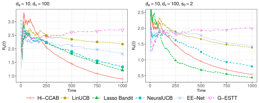
Figure 8: Expected average regret.

In Kang et al., (2022), the main algorithm with theoretical guarantees is designed for low-rank matrix bandit but not for contextual bandit. In Appendix H, the author sketched an extension to the contextual setting, but their theory and numerical validation only apply to non-contextual bandits. We applied the modified G-ESTT to the contextual bandit setting where $d_{a}=10,d_{x}=100$ and the sparse setting with $d_{a}=10,d_{x}=100,s_{0}=2$ as in Section 5.2. Figure 8 shows that the modified G-ESTT does not perform well compared to other contextual bandit algorithms. One reason can be the following. They adopt the explore-then-commit algorithm and their initialization step is required to be of the order $\sqrt{d_{1}d_{2}rT}$. In our simulation setting, the dimension of covariate $d_{2}=d_{x}$ is high and therefore their algorithm will require a large $T_{1}$ to perform well. Therefore, the modified G-ESTT does not perform well in high-dimensional settings (note that the dimensions in their simulations is of the order 10), especially when $T$ is relatively small. In addition, the computational complexity of the modified G-ESTT is high compared to other methods. We tried to run the modified G-ESTT for other settings as in Section 5.2 with larger $d_{x}$ but it would have taken too long and we do not expect a better performance of the modified G-ESTT in higher dimension settings given the above-mentioned claim.

9.2 More details on Case Study I

In this section, we provides more background information on Case Study I and additional numerical results.

Figure 9(a) shows the daily sales by product and each color represents one product (only products that appeared more than 95% of the days are colored; the rest are colored as grey). The days corresponding to the vertical dashed grey lines are days with promotion. The two red vertical lines correspond to the annual sales events. The variation between products was large and one product dominated the rest most of the time. The sales were also driven by the promotion – the sales went up when there is a promotion. Figure 9(b) shows the median unit price across time with the 25th and 75th quantiles as the boundaries of the grey area. The median unit price was around 3.2 RMB and there were variations in unit price among products. Figure 9(c) shows the number of single-flavor and multi-flavor products. Three-quarters of the products were single-flavored. Note that products with the same flavor can have different package sizes. Figure 9(d) shows the number of products with different package sizes. The package size of about 60% of the products is larger than 20 with 30% having package sizes between 10 and 20 and the rest less than 10.

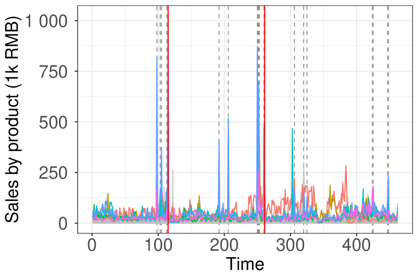
(a) Total sales by product in 1k RMB.

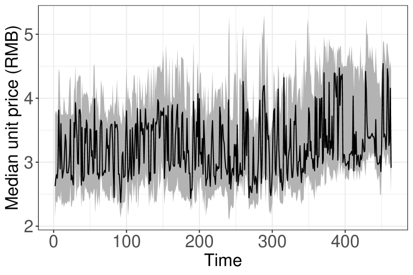
(b) Median price of products.

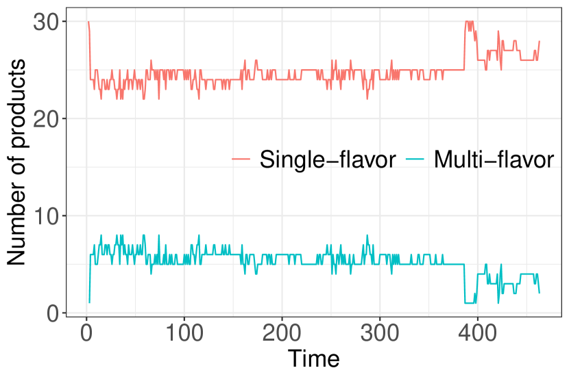
(c) Number of products with various number of flavors.

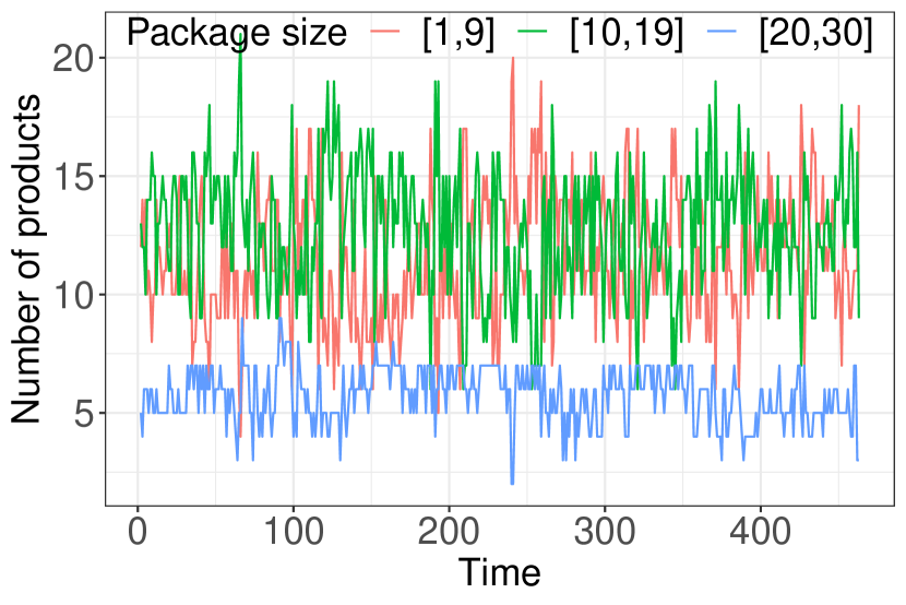
(d) Number of products with various package sizes.

Figure 9: Summary of the products.

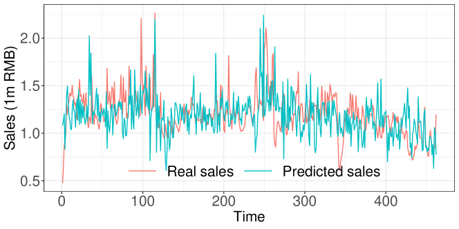
Figure 10: Real sales vs predicted sales.

To check our model assumption (3) on the data, Figure 10 shows the hold-out-sample prediction of the sales versus the real sales. The predicted sale at each time point $t$ is the predicted total sales across $L=31$ locations based on $\widehat{\bm{\Theta}}_{-t}$ estimated from all the data except for data at time $t$, i.e.,

$$\hat{y}_{t,\ell}={\bm{a}}_{t}^{\top}\widehat{{\bm{\Theta}}}_{-t}{\bm{x}}_{t,\ell},$$

where $\widehat{{\bm{\Theta}}}_{-t}=\arg\min_{{\bm{\Theta}}}\sum_{i=1,i\neq t}^{T}\sum_{\ell=1}^{L}\left({\bm{a}}_{i}^{\top}{\bm{\Theta}}{\bm{x}}_{i,\ell}-r_{i,\ell}\right)^{2}+\lambda|\!|\!|{\bm{\Theta}}|\!|\!|_{{\footnotesize{\mbox{nuc}}}}$. As shown in Figure 10, the real sales and the out-of-sample predicted sales follow quite closely across time and the out-of-sample prediction error rate $\sum_{i=1}^{T}\sum_{\ell=1}^{L}(y_{t,\ell}-\hat{y}_{t,\ell})^{2}/\sum_{i=1}^{T}\sum_{\ell=1}^{L}y_{t,\ell}^{2}=0.07$, which indicates that both our model and estimation are reasonable.

Further simulation results.

We first detail how we ran the simulation and then provide more simulation results.

We run 100 trials, in each of which we set $t_{\mathchoice{\raisebox{0.0pt}{\leavevmode\resizebox{10.00948pt}{4.0pt}{\hbox{\raisebox{0.0pt}{$\displaystyle init$}}}}}{\raisebox{0.0pt}{\leavevmode\resizebox{10.00948pt}{4.0pt}{\hbox{\raisebox{0.0pt}{$\textstyle init$}}}}}{\raisebox{0.0pt}{\leavevmode\resizebox{10.00948pt}{4.0pt}{\hbox{\raisebox{0.0pt}{$\scriptstyle init$}}}}}{\raisebox{0.0pt}{\leavevmode\resizebox{10.00945pt}{4.0pt}{\hbox{\raisebox{0.0pt}{$\scriptscriptstyle init$}}}}}}=100$ for the initialization step and $\lambda_{0}$ according to Algorithm 1 to estimate $\widehat{\bm{\Theta}}_{t_{\mathchoice{\raisebox{0.0pt}{\leavevmode\resizebox{10.00946pt}{4.0pt}{\hbox{\raisebox{0.0pt}{$\displaystyle init$}}}}}{\raisebox{0.0pt}{\leavevmode\resizebox{10.00946pt}{4.0pt}{\hbox{\raisebox{0.0pt}{$\textstyle init$}}}}}{\raisebox{0.0pt}{\leavevmode\resizebox{10.00945pt}{4.0pt}{\hbox{\raisebox{0.0pt}{$\scriptstyle init$}}}}}{\raisebox{0.0pt}{\leavevmode\resizebox{10.00948pt}{4.0pt}{\hbox{\raisebox{0.0pt}{$\scriptscriptstyle init$}}}}}}}$; and then at each time $t=t_{\mathchoice{\raisebox{0.0pt}{\leavevmode\resizebox{10.00948pt}{4.0pt}{\hbox{\raisebox{0.0pt}{$\displaystyle init$}}}}}{\raisebox{0.0pt}{\leavevmode\resizebox{10.00948pt}{4.0pt}{\hbox{\raisebox{0.0pt}{$\textstyle init$}}}}}{\raisebox{0.0pt}{\leavevmode\resizebox{10.00948pt}{4.0pt}{\hbox{\raisebox{0.0pt}{$\scriptstyle init$}}}}}{\raisebox{0.0pt}{\leavevmode\resizebox{10.00945pt}{4.0pt}{\hbox{\raisebox{0.0pt}{$\scriptscriptstyle init$}}}}}}+1,\ldots,T$, we follow Algorithm 1 to make an assortment-pricing decide ${\bm{a}}_{t}$ given covariate ${\bm{x}}_{t}$. After determining ${\bm{a}}_{t}$, we generate the sales $y_{t,\ell}$ for $\ell=1,\ldots,L=31$ locations according to model (3) based on the pseudo-truth-model with $({\bm{\Theta}},\sigma)$. We further compare the performance of the assortment-pricing policy with exploration and without exploration and with different initialization time $t_{\mathchoice{\raisebox{0.0pt}{\leavevmode\resizebox{10.00948pt}{4.0pt}{\hbox{\raisebox{0.0pt}{$\displaystyle init$}}}}}{\raisebox{0.0pt}{\leavevmode\resizebox{10.00948pt}{4.0pt}{\hbox{\raisebox{0.0pt}{$\textstyle init$}}}}}{\raisebox{0.0pt}{\leavevmode\resizebox{10.00948pt}{4.0pt}{\hbox{\raisebox{0.0pt}{$\scriptstyle init$}}}}}{\raisebox{0.0pt}{\leavevmode\resizebox{10.00945pt}{4.0pt}{\hbox{\raisebox{0.0pt}{$\scriptscriptstyle init$}}}}}}$. Each setup is simulated 100 times.

Figures 11(a)-11(b) show the time-averaged regret and Figure 11(d) show percentage gain in cumulative sales when $t_{\mathchoice{\raisebox{0.0pt}{\leavevmode\resizebox{10.00948pt}{4.0pt}{\hbox{\raisebox{0.0pt}{$\displaystyle init$}}}}}{\raisebox{0.0pt}{\leavevmode\resizebox{10.00948pt}{4.0pt}{\hbox{\raisebox{0.0pt}{$\textstyle init$}}}}}{\raisebox{0.0pt}{\leavevmode\resizebox{10.00948pt}{4.0pt}{\hbox{\raisebox{0.0pt}{$\scriptstyle init$}}}}}{\raisebox{0.0pt}{\leavevmode\resizebox{10.00945pt}{4.0pt}{\hbox{\raisebox{0.0pt}{$\scriptscriptstyle init$}}}}}}=20,50,100$ with exploration and without exploration. Hi-CCAB with exploration performs better then without exploration. As expected, longer initialization steps provide a better initial estimation of the ${\bm{\Theta}}$ and thus helps with the performance in a short time windows. As time goes by, all of the time-averaged regrets converge to zero and the percentage gain in cumulative sales should converge.

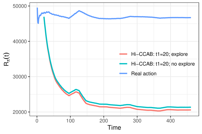
(a) Time-averaged regret when $t_{\mathchoice{\raisebox{0.0pt}{\leavevmode\resizebox{10.00948pt}{4.0pt}{\hbox{\raisebox{0.0pt}{$\displaystyle init$}}}}}{\raisebox{0.0pt}{\leavevmode\resizebox{10.00948pt}{4.0pt}{\hbox{\raisebox{0.0pt}{$\textstyle init$}}}}}{\raisebox{0.0pt}{\leavevmode\resizebox{10.00946pt}{4.0pt}{\hbox{\raisebox{0.0pt}{$\scriptstyle init$}}}}}{\raisebox{0.0pt}{\leavevmode\resizebox{10.00941pt}{4.0pt}{\hbox{\raisebox{0.0pt}{$\scriptscriptstyle init$}}}}}}=20$.

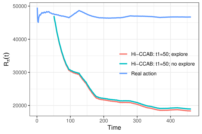
(b) Time-averaged when $t_{\mathchoice{\raisebox{0.0pt}{\leavevmode\resizebox{10.00948pt}{4.0pt}{\hbox{\raisebox{0.0pt}{$\displaystyle init$}}}}}{\raisebox{0.0pt}{\leavevmode\resizebox{10.00948pt}{4.0pt}{\hbox{\raisebox{0.0pt}{$\textstyle init$}}}}}{\raisebox{0.0pt}{\leavevmode\resizebox{10.00946pt}{4.0pt}{\hbox{\raisebox{0.0pt}{$\scriptstyle init$}}}}}{\raisebox{0.0pt}{\leavevmode\resizebox{10.00941pt}{4.0pt}{\hbox{\raisebox{0.0pt}{$\scriptscriptstyle init$}}}}}}=50$.

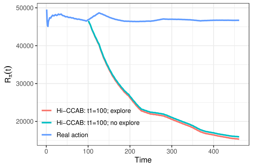
(c) Time-averaged when $t_{\mathchoice{\raisebox{0.0pt}{\leavevmode\resizebox{10.00948pt}{4.0pt}{\hbox{\raisebox{0.0pt}{$\displaystyle init$}}}}}{\raisebox{0.0pt}{\leavevmode\resizebox{10.00948pt}{4.0pt}{\hbox{\raisebox{0.0pt}{$\textstyle init$}}}}}{\raisebox{0.0pt}{\leavevmode\resizebox{10.00946pt}{4.0pt}{\hbox{\raisebox{0.0pt}{$\scriptstyle init$}}}}}{\raisebox{0.0pt}{\leavevmode\resizebox{10.00941pt}{4.0pt}{\hbox{\raisebox{0.0pt}{$\scriptscriptstyle init$}}}}}}=100$.

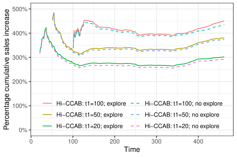
(d) Percentage cumulative sales gain.

Figure 11: Performance of Hi-CCAB with different initialization times $t_{\mathchoice{\raisebox{0.0pt}{\leavevmode\resizebox{10.00948pt}{4.0pt}{\hbox{\raisebox{0.0pt}{$\displaystyle init$}}}}}{\raisebox{0.0pt}{\leavevmode\resizebox{10.00948pt}{4.0pt}{\hbox{\raisebox{0.0pt}{$\textstyle init$}}}}}{\raisebox{0.0pt}{\leavevmode\resizebox{10.00946pt}{4.0pt}{\hbox{\raisebox{0.0pt}{$\scriptstyle init$}}}}}{\raisebox{0.0pt}{\leavevmode\resizebox{10.00941pt}{4.0pt}{\hbox{\raisebox{0.0pt}{$\scriptscriptstyle init$}}}}}}$ and with and without exploration.

9.3 More details on Case Study II

In this section, we provides more background information on Case Study II and additional numerical results.

Figure 12(a) shows the total counts of manicures featuring various colors. Note that one manicure can potentially use multiple colors. Red was the most prevalent color, followed by white, gray, black, blue, yellow, and orange. The ranking, apart from red, was determined by sales volumes from previous periods. Figure 12(b) shows the style of the manicures, i.e., percentages of designer, glossy, and transparent manicures respectively. The count of designer manicures surged in around June 2020 after the total profits increased and then plateaued as shown in Figure 13. Figure 12(c) shows the total number of followers on Instagram of the designers and Figure 12(d) presents the discount rate, calculated as the percentage of total daily discount amounts. Notably, discount peaks are observed around Thanksgiving, New Year’s, and April Fool’s Day.

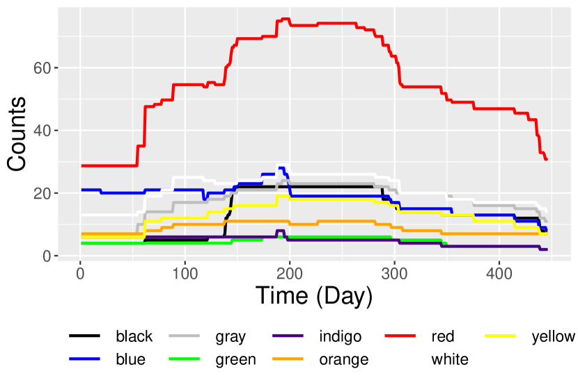
(a) Counts of manicures with different colors.

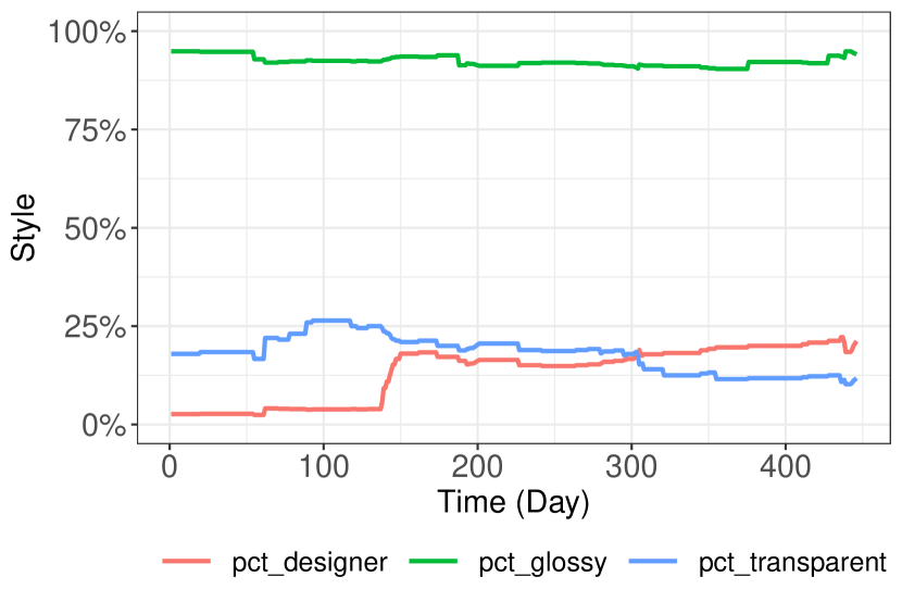
(b) Style of the manicures.

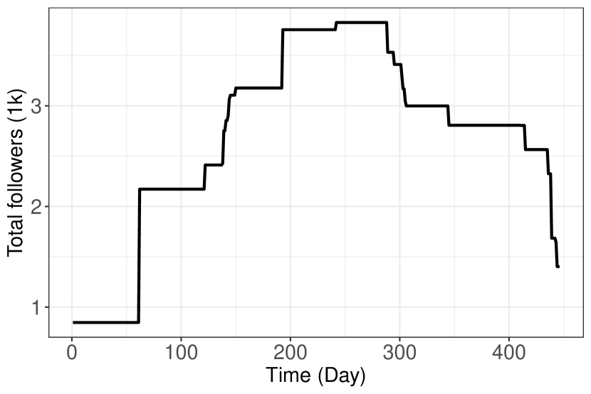
(c) Total number of follows of designers.

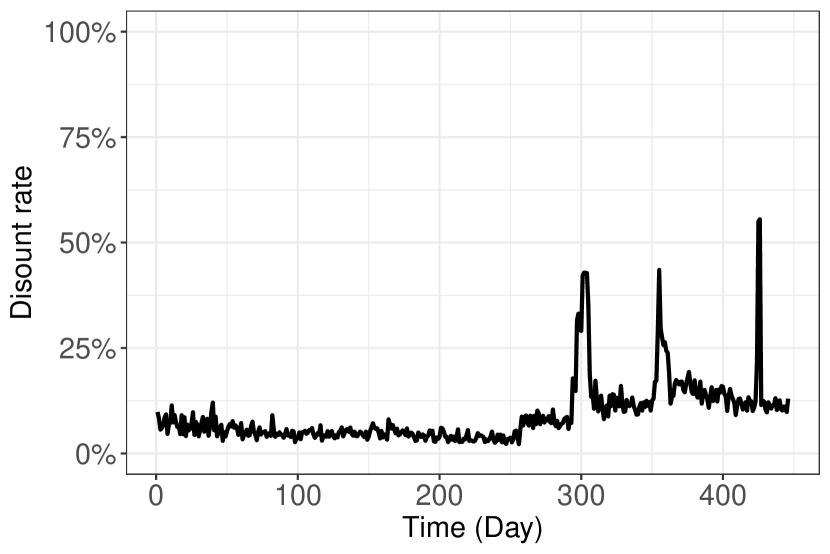
(d) Discount rate.

Figure 12: Summary of the products.

We check our model assumption (3) on the data similar to Case Study I as detailed in Section 9.2. Figure 10 shows the hold-out-sample prediction of the profits versus the real profits. The real sales and the out-of-sample predicted sales follow quite closely over time and the out-of-sample prediciton error rate is around 8%, which again indicates that both our model and estimation are reasonable.

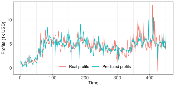
Figure 13: Real profits vs predicted profits.

References

- Abbasi-Yadkori et al., (2011) Abbasi-Yadkori, Y., Pál, D., and Szepesvári, C. (2011). Improved algorithms for linear stochastic bandits. In Advances in Neural Information Processing Systems, volume 24.
- Abbasi-Yadkori et al., (2012) Abbasi-Yadkori, Y., Pal, D., and Szepesvari, C. (2012). Online-to-confidence-set conversions and application to sparse stochastic bandits. In Artificial Intelligence and Statistics, pages 1–9. PMLR.
- Agrawal, (1995) Agrawal, R. (1995). The continuum-armed bandit problem. SIAM journal on control and optimization, 33(6):1926–1951.
- Agrawal et al., (2019) Agrawal, S., Avadhanula, V., Goyal, V., and Zeevi, A. (2019). MNL-bandit: A dynamic learning approach to assortment selection. Operations Research, 67(5):1453–1485.
- Akçay et al., (2010) Akçay, Y., Natarajan, H. P., and Xu, S. H. (2010). Joint dynamic pricing of multiple perishable products under consumer choice. Management Science, 56(8):1345–1361.
- Araman and Caldentey, (2009) Araman, V. F. and Caldentey, R. (2009). Dynamic pricing for nonperishable products with demand learning. Operations Research, 57(5):1169–1188.
- Auer, (2002) Auer, P. (2002). Using confidence bounds for exploitation-exploration trade-offs. Journal of Machine Learning Research, 3(Nov):397–422.
- Ban and Keskin, (2021) Ban, G.-Y. and Keskin, N. B. (2021). Personalized dynamic pricing with machine learning: High-dimensional features and heterogeneous elasticity. Management Science, 67(9):5549–5568.
- Ban et al., (2022) Ban, Y., Yan, Y., Banerjee, A., and He, J. (2022). EE-net: Exploitation-exploration neural networks in contextual bandits. In The Tenth International Conference on Learning Representations.
- Bastani and Bayati, (2020) Bastani, H. and Bayati, M. (2020). Online decision making with high-dimensional covariates. Operations Research, 68(1):276–294.
- Bastani et al., (2022) Bastani, H., Simchi-Levi, D., and Zhu, R. (2022). Meta dynamic pricing: Transfer learning across experiments. Management Science, 68(3):1865–1881.
- Bennett et al., (2007) Bennett, J., Lanning, S., et al. (2007). The Netflix prize. In Proceedings of KDD cup and workshop, volume 2007, page 35. New York.
- Bernstein et al., (2019) Bernstein, F., Modaresi, S., and Sauré, D. (2019). A dynamic clustering approach to data-driven assortment personalization. Management Science, 65(5):2095–2115.
- Besbes and Zeevi, (2009) Besbes, O. and Zeevi, A. (2009). Dynamic pricing without knowing the demand function: Risk bounds and near-optimal algorithms. Operations Research, 57(6):1407–1420.
- Boucheron et al., (2013) Boucheron, S., Lugosi, G., and Massart, P. (2013). Concentration Inequalities: A Nonasymptotic Theory of Independence. Oxford University Press.
- Broder and Rusmevichientong, (2012) Broder, J. and Rusmevichientong, P. (2012). Dynamic pricing under a general parametric choice model. Operations Research, 60(4):965–980.
- Cai and Guo, (2017) Cai, T. T. and Guo, Z. (2017). Confidence intervals for high-dimensional linear regression: Minimax rates and adaptivity. The Annals of Statistics, 45(2):615 – 646.
- Cai and Zhang, (2018) Cai, T. T. and Zhang, A. (2018). Rate-optimal perturbation bounds for singular subspaces with applications to high-dimensional statistics. The Annals of Statistics, 46(1):60–89.
- Candes and Plan, (2010) Candes, E. J. and Plan, Y. (2010). Matrix completion with noise. Proceedings of the IEEE, 98(6):925–936.
- Caro and Gallien, (2007) Caro, F. and Gallien, J. (2007). Dynamic assortment with demand learning for seasonal consumer goods. Management science, 53(2):276–292.
- Chen and Gallego, (2021) Chen, N. and Gallego, G. (2021). Nonparametric pricing analytics with customer covariates. Operations Research, 69(3):974–984.
- Chen et al., (2023) Chen, X., Krishnamurthy, A., and Wang, Y. (2023). Robust dynamic assortment optimization in the presence of outlier customers. Operations Research.
- (23) Chen, X., Owen, Z., Pixton, C., and Simchi-Levi, D. (2022a). A statistical learning approach to personalization in revenue management. Management Science, 68(3):1923–1937.
- Chen et al., (2021) Chen, X., Shi, C., Wang, Y., and Zhou, Y. (2021). Dynamic assortment planning under nested logit models. Production and Operations Management, 30(1):85–102.
- Chen and Wang, (2017) Chen, X. and Wang, Y. (2017). A note on a tight lower bound for mnl-bandit assortment selection models. arXiv preprint arXiv:1709.06109.
- Chen et al., (2020) Chen, X., Wang, Y., and Zhou, Y. (2020). Dynamic assortment optimization with changing contextual information. The Journal of Machine Learning Research, 21(1):8918–8961.
- (27) Chen, Y., Wang, Y., Fang, E. X., Wang, Z., and Li, R. (2022b). Nearly dimension-independent sparse linear bandit over small action spaces via best subset selection. Journal of the American Statistical Association, pages 1–13.
- (28) Chen, Y., Xie, M., Liu, J., and Zhao, K. (2022c). Interconnected neural linear contextual bandits with UCB exploration. In Pacific-Asia Conference on Knowledge Discovery and Data Mining, pages 169–181. Springer.
- Cheung and Simchi-Levi, (2017) Cheung, W. C. and Simchi-Levi, D. (2017). Thompson sampling for online personalized assortment optimization problems with multinomial logit choice models. Available at SSRN 3075658.
- Cohen et al., (2020) Cohen, M. C., Lobel, I., and Paes Leme, R. (2020). Feature-based dynamic pricing. Management Science, 66(11):4921–4943.
- Dani et al., (2008) Dani, V., Hayes, T. P., and Kakade, S. M. (2008). Stochastic linear optimization under bandit feedback. In Conference on Learning Theory.
- Den Boer, (2015) Den Boer, A. V. (2015). Dynamic pricing and learning: historical origins, current research, and new directions. Surveys in Operations Research and Management Science, 20(1):1–18.
- den Boer and Zwart, (2014) den Boer, A. V. and Zwart, B. (2014). Simultaneously learning and optimizing using controlled variance pricing. Management Science, 60(3):770–783.
- Estelami et al., (2001) Estelami, H., Lehmann, D. R., and Holden, A. C. (2001). Macro-economic determinants of consumer price knowledge: A meta-analysis of four decades of research. International Journal of Research in Marketing, 18(4):341–355.
- Fan et al., (2022) Fan, J., Guo, Y., and Yu, M. (2022). Policy optimization using semiparametric models for dynamic pricing. Journal of the American Statistical Association, pages 1–29.
- Fan et al., (2021) Fan, J., Li, K., and Liao, Y. (2021). Recent developments in factor models and applications in econometric learning. Annual Review of Financial Economics, 13:401–430.
- Féraud et al., (2016) Féraud, R., Allesiardo, R., Urvoy, T., and Clérot, F. (2016). Random forest for the contextual bandit problem. In Artificial Intelligence and Statistics, pages 93–101. PMLR.
- Foupouagnigni and Mouafo Wouodjié, (2020) Foupouagnigni, M. and Mouafo Wouodjié, M. (2020). On multivariate Bernstein polynomials. Mathematics, 8(9):1397.
- Gallego and Wang, (2014) Gallego, G. and Wang, R. (2014). Multiproduct price optimization and competition under the nested logit model with product-differentiated price sensitivities. Operations Research, 62(2):450–461.
- Gordon et al., (2013) Gordon, B. R., Goldfarb, A., and Li, Y. (2013). Does price elasticity vary with economic growth? a cross-category analysis. Journal of Marketing Research, 50(1):4–23.
- Hao et al., (2020) Hao, B., Lattimore, T., and Wang, M. (2020). High-dimensional sparse linear bandits. In Advances in Neural Information Processing Systems, volume 33, pages 10753–10763.
- Hotelling, (1933) Hotelling, H. (1933). Analysis of a complex of statistical variables into principal components. Journal of Educational Psychology, 24(6):417.
- Hu et al., (2021) Hu, J., Chen, X., Jin, C., Li, L., and Wang, L. (2021). Near-optimal representation learning for linear bandits and linear RL. In International Conference on Machine Learning, pages 4349–4358. PMLR.
- Javanmard and Nazerzadeh, (2019) Javanmard, A. and Nazerzadeh, H. (2019). Dynamic pricing in high-dimensions. The Journal of Machine Learning Research, 20(1):315–363.
- Jun et al., (2019) Jun, K.-S., Willett, R., Wright, S., and Nowak, R. (2019). Bilinear bandits with low-rank structure. In International Conference on Machine Learning, pages 3163–3172. PMLR.
- Kaiser, (1958) Kaiser, H. F. (1958). The Varimax criterion for analytic rotation in factor analysis. Psychometrika, 23(3):187–200.
- Kallus and Udell, (2020) Kallus, N. and Udell, M. (2020). Dynamic assortment personalization in high dimensions. Operations Research, 68(4):1020–1037.
- Kang et al., (2022) Kang, Y., Hsieh, C.-J., and Lee, T. C. M. (2022). Efficient frameworks for generalized low-rank matrix bandit problems. In Advances in Neural Information Processing Systems, volume 35, pages 19971–19983.
- Keskin and Zeevi, (2014) Keskin, N. B. and Zeevi, A. (2014). Dynamic pricing with an unknown demand model: Asymptotically optimal semi-myopic policies. Operations research, 62(5):1142–1167.
- Kim and Paik, (2019) Kim, G.-S. and Paik, M. C. (2019). Doubly-robust LASSO bandit. In Advances in Neural Information Processing Systems, volume 32.
- Kim and Vojnovic, (2021) Kim, J.-h. and Vojnovic, M. (2021). Scheduling servers with stochastic bilinear rewards. arXiv preprint arXiv:2112.06362.
- Kleinberg, (2004) Kleinberg, R. (2004). Nearly tight bounds for the continuum-armed bandit problem. In Proceedings of the 17th International Conference on Neural Information Processing Systems, NIPS’04, pages 697––704, Cambridge, MA, USA. MIT Press.
- Kleinberg and Leighton, (2003) Kleinberg, R. and Leighton, T. (2003). The value of knowing a demand curve: Bounds on regret for online posted-price auctions. In 44th Annual IEEE Symposium on Foundations of Computer Science, 2003. Proceedings., pages 594–605. IEEE.
- Kleinberg et al., (2019) Kleinberg, R., Slivkins, A., and Upfal, E. (2019). Bandits and experts in metric spaces. Journal of the ACM, 66(4).
- Krishnamurthy et al., (2020) Krishnamurthy, A., Langford, J., Slivkins, A., and Zhang, C. (2020). Contextual bandits with continuous actions: Smoothing, zooming, and adapting. The Journal of Machine Learning Research, 21(1):5402–5446.
- Kumar et al., (2014) Kumar, V., Umashankar, N., Kim, K. H., and Bhagwat, Y. (2014). Assessing the influence of economic and customer experience factors on service purchase behaviors. Marketing Science, 33(5):673–692.
- Kveton et al., (2017) Kveton, B., Szepesvári, C., Rao, A., Wen, Z., Abbasi-Yadkori, Y., and Muthukrishnan, S. (2017). Stochastic low-rank bandits. arXiv preprint arXiv:1712.04644.
- Lale et al., (2019) Lale, S., Azizzadenesheli, K., Anandkumar, A., and Hassibi, B. (2019). Stochastic linear bandits with hidden low rank structure. arXiv preprint arXiv:1901.09490.
- Lattimore and Szepesvári, (2020) Lattimore, T. and Szepesvári, C. (2020). Bandit algorithms. Cambridge University Press.
- Laurent and Massart, (2000) Laurent, B. and Massart, P. (2000). Adaptive estimation of a quadratic functional by model selection. Annals of Statistics, pages 1302–1338.
- Li et al., (2010) Li, L., Chu, W., Langford, J., and Schapire, R. E. (2010). A contextual-bandit approach to personalized news article recommendation. In Proceedings of the 19th International Conference on World Wide Web, pages 661–670.
- Li et al., (2018) Li, Q., Cheng, G., Fan, J., and Wang, Y. (2018). Embracing the blessing of dimensionality in factor models. Journal of the American Statistical Association, 113(521):380–389.
- Lu et al., (2010) Lu, T., Pál, D., and Pál, M. (2010). Contextual multi-armed bandits. In Proceedings of the Thirteenth International Conference on Artificial Intelligence and Statistics, pages 485–492. JMLR Workshop and Conference Proceedings.
- Lu et al., (2021) Lu, Y., Meisami, A., and Tewari, A. (2021). Low-rank generalized linear bandit problems. In International Conference on Artificial Intelligence and Statistics, pages 460–468. PMLR.
- Madden et al., (2000) Madden, T. J., Hewett, K., and Roth, M. S. (2000). Managing images in different cultures: A cross-national study of color meanings and preferences. Journal of International Marketing, 8(4):90–107.
- Miao and Chao, (2021) Miao, S. and Chao, X. (2021). Dynamic joint assortment and pricing optimization with demand learning. Manufacturing & Service Operations Management, 23(2):525–545.
- Miao and Chao, (2022) Miao, S. and Chao, X. (2022). Online personalized assortment optimization with high-dimensional customer contextual data. Manufacturing & Service Operations Management, 24(5):2741–2760.
- Miao et al., (2022) Miao, S., Chen, X., Chao, X., Liu, J., and Zhang, Y. (2022). Context-based dynamic pricing with online clustering. Production and Operations Management, 31(9):3559–3575.
- Negahban and Wainwright, (2011) Negahban, S. and Wainwright, M. J. (2011). Estimation of (near) low-rank matrices with noise and high-dimensional scaling. The Annals of Statistics, 39(2):1069–1097.
- Papini et al., (2021) Papini, M., Tirinzoni, A., Restelli, M., Lazaric, A., and Pirotta, M. (2021). Leveraging good representations in linear contextual bandits. In International Conference on Machine Learning, pages 8371–8380. PMLR.
- Pol, (1991) Pol, L. G. (1991). Demographic contributions to marketing: an assessment. Journal of the Academy of Marketing Science, 19:53–59.
- Qiang and Bayati, (2016) Qiang, S. and Bayati, M. (2016). Dynamic pricing with demand covariates. arXiv preprint arXiv:1604.07463.
- Recht et al., (2010) Recht, B., Fazel, M., and Parrilo, P. A. (2010). Guaranteed minimum-rank solutions of linear matrix equations via nuclear norm minimization. SIAM Review, 52(3):471–501.
- Rizk et al., (2021) Rizk, G., Thomas, A., Colin, I., Laraki, R., and Chevaleyre, Y. (2021). Best arm identification in graphical bilinear bandits. In International Conference on Machine Learning, pages 9010–9019. PMLR.
- Robbins, (1952) Robbins, H. (1952). Some aspects of the sequential design of experiments. Bulletin of the American Mathematical Society, 58(5):527–535.
- Rohe and Zeng, (2023) Rohe, K. and Zeng, M. (2023). Vintage Factor Analysis with Varimax Performs Statistical Inference. Journal of the Royal Statistical Society Series B: Statistical Methodology, page qkad029.
- Rusmevichientong et al., (2010) Rusmevichientong, P., Shen, Z.-J. M., and Shmoys, D. B. (2010). Dynamic assortment optimization with a multinomial logit choice model and capacity constraint. Operations Research, 58(6):1666–1680.
- Rusmevichientong and Tsitsiklis, (2010) Rusmevichientong, P. and Tsitsiklis, J. N. (2010). Linearly parameterized bandits. Mathematics of Operations Research, 35(2):395–411.
- Sauré and Zeevi, (2013) Sauré, D. and Zeevi, A. (2013). Optimal dynamic assortment planning with demand learning. Manufacturing & Service Operations Management, 15(3):387–404.
- Schuler et al., (2016) Schuler, A., Liu, V., Wan, J., Callahan, A., Udell, M., Stark, D. E., and Shah, N. H. (2016). Discovering patient phenotypes using generalized low rank models. In Biocomputing 2016: Proceedings of the Pacific Symposium, pages 144–155. World Scientific.
- Shen et al., (2023) Shen, S., Chen, X., Fang, E., and Lu, J. (2023). Combinatorial inference on the optimal assortment in multinomial logit models. Available at SSRN 4371919.
- Singh, (2006) Singh, S. (2006). Impact of color on marketing. Management Decision, 44(6):783–789.
- Slivkins, (2011) Slivkins, A. (2011). Contextual bandits with similarity information. In Proceedings of the 24th annual Conference On Learning Theory, pages 679–702. JMLR Workshop and Conference Proceedings.
- Srebro et al., (2005) Srebro, N., Alon, N., and Jaakkola, T. S. (2005). Generalization error bounds for collaborative prediction with low-rank matrices. In Neural Information Processing Systems (NIPS).
- Tropp, (2012) Tropp, J. A. (2012). User-friendly tail bounds for sums of random matrices. Foundations of Computational Mathematics, 12(4):389–434.
- Turğay et al., (2020) Turğay, E., Bulucu, C., and Tekin, C. (2020). Exploiting relevance for online decision-making in high-dimensions. IEEE Transactions on Signal Processing, 69:1438–1451.
- Udell et al., (2016) Udell, M., Horn, C., Zadeh, R., Boyd, S., et al. (2016). Generalized low rank models. Foundations and Trends® in Machine Learning, 9(1):1–118.
- Wainwright, (2019) Wainwright, M. J. (2019). High-dimensional statistics: A non-asymptotic viewpoint, volume 48. Cambridge University Press.
- Wakefield and Inman, (2003) Wakefield, K. L. and Inman, J. J. (2003). Situational price sensitivity: the role of consumption occasion, social context and income. Journal of Retailing, 79(4):199–212.
- Xu and Bastani, (2021) Xu, K. and Bastani, H. (2021). Learning across bandits in high dimension via robust statistics. arXiv preprint arXiv:2112.14233.
- Xu et al., (2022) Xu, P., Wen, Z., Zhao, H., and Gu, Q. (2022). Neural contextual bandits with deep representation and shallow exploration. In The Tenth International Conference on Learning Representations.
- Yang et al., (2020) Yang, J., Hu, W., Lee, J. D., and Du, S. S. (2020). Impact of representation learning in linear bandits. arXiv preprint arXiv:2010.06531.
- Zhou et al., (2020) Zhou, D., Li, L., and Gu, Q. (2020). Neural contextual bandits with UCB-based exploration. In International Conference on Machine Learning, pages 11492–11502. PMLR.