Representation Learning in Low-rank Slate-based Recommender Systems
Abstract
Reinforcement learning (RL) in recommendation systems offers the potential to optimize recommendations for long-term user engagement. However, the environment often involves large state and action spaces, which makes it hard to efficiently learn and explore. In this work, we propose a sample-efficient representation learning algorithm, using the standard slate recommendation setup, to treat this as an online RL problem with low-rank Markov decision processes (MDPs). We also construct the recommender simulation environment with the proposed setup and sampling method.
1 Introduction
Recommender systems aim to find personalized contents based on the learned user preferences, as in collaborative filtering (Breese et al., 2013; Konstan et al., 1997; Srebro et al., 2004; Mnih & Salakhutdinov, 2007) and content-based filtering (Van Meteren & Van Someren, 2000). A good recommender increases user engagement, and keeps the user interacting within the system. The current popular platforms, like Youtube (Covington et al., 2016), Spotify (Jacobson et al., 2016), and Netflix (Gomez-Uribe & Hunt, 2015), make extensive use of recommender systems. However, as a user interacts with the system for a longer term, it becomes necessary to keep track of the user dynamics. Traditional methods focus more on myopic predictions, where they estimate the users’ immediate responses. Current research has increased to narrate the problem as a Markov decision process (Rendle et al., 2010; He & McAuley, 2016), and do long-term planning using reinforcement learning algorithms (Shani et al., 2005; Gauci et al., 2018). However, using RL methods in recommender systems faces an issue regarding the large observation and action space, and doing efficient exploration becomes a harder question. Prior RL methods in recommender systems often overlook exploration, or use -greedy and Boltzmann exploration (Afsar et al., 2022).
In this work, we do representation learning under the low-rank MDP assumption. More specifically, we focus on the case where a user can be learned using a history of observations into a low-dimension representation. And the user dynamics can be modeled as transitions of such representation. Concretely, a low-rank MDP assumes that the MDP transition matrix admits a low-rank factorization, i.e., there exists two unknown mappings , , such that for all , where is the probability of transiting to the next state under the current state and action . The representation in a low-rank MDP not only linearizes the optimal state-action value function of the MDP (Jin et al., 2020), but also linearizes the transition operator. Such low-rankness assumption has been shown to be realistic in movie recommender systems (Koren et al., 2009).
Our main contribution is using upper confidence bound (UCB) driven representation learning to efficiently explore in user representation space. It is a practical extension from Rep-UCB, which provides theorical guarantee on efficient exploration under low-rank MDP with sample complexity (Uehara et al., 2021). We focus on the case where action is slate recommendation. And under the mild assumption of user choice behavior which we will elaborate in Definition 2.3, the combinatorial action space can be reduced to where is the slate size and is the item space.
To evaluate our method systematically, we introduce a recommender simulation environment, RecSim NG, that allows the straightforward configuration of an item collection (or vocabulary), a user (latent) state model and a user choice model (Mladenov et al., 2021). We describe specific instantiations of this environment suitable for user representation learning, and the construction of our Rep-UCB-Rec learning and optimization methods.
1.1 Related Works
Recommender Systems Recommender systems have relied on collaborative filtering techniques to learn the connection between users and items. Conceptually, they cluster users and items, or embed users and items in a low-dimensional representation (Krestel et al., 2009; Moshfeghi et al., 2011) for further predictions.
For the sake of capturing more nuanced user behaviors, deep neural networks (DNNs) are used in real world applications (Van den Oord et al., 2013; Covington et al., 2016). It naturally follows to be studied as a RL problem, as the user dynamics can be modeled as MDPs. Embeddings are commonly used to learn latent representations from immediate user interactions (Liu et al., 2020). And predictive models are commonly used to improve sample efficiency (Chen et al., 2021) and do self-supervised RL (Xin et al., 2020; Zhou et al., 2020).
Low-rank MDPs Oracle-efficient algorithms for low-rank MDPs (Agarwal et al., 2020; Uehara et al., 2021) provide sample complexity bounds easing the difficulty of exploration in large state space. Under more restricted setting, such as block MDPs (Misra et al., 2020) and -step decodable MDPs (Efroni et al., 2022), methods are also studied to deal with the curse of dimensionality.
Slate-based recommendation and choice models Slate recommondation is common in recommender systems (Deshpande & Karypis, 2004; Viappiani & Boutilier, 2010; Ie et al., 2019). Within the context, the complexity within a constructed plate is studied using methods like off-policy evaluation and learning inverse propensity scores (Swaminathan et al., 2017). Hierarchical models are also used for studying user behavior interacting with slates (Mehrotra et al., 2019).
The user choice model is linked with the slate recommendation. A common choice model is multinomial logit model (Louviere et al., 2000). As a good representation of user choice boosts the probability capturing the real-world user behaviors, many areas, such as econometrics, psychology, and operations research (Luce, 2012), have studied it using their own scientific methods. Within the ML community, another popular choice is cascade model (Joachims, 2002), as it also captures the fading attention introduced by browsing behavior.
2 Preliminaries
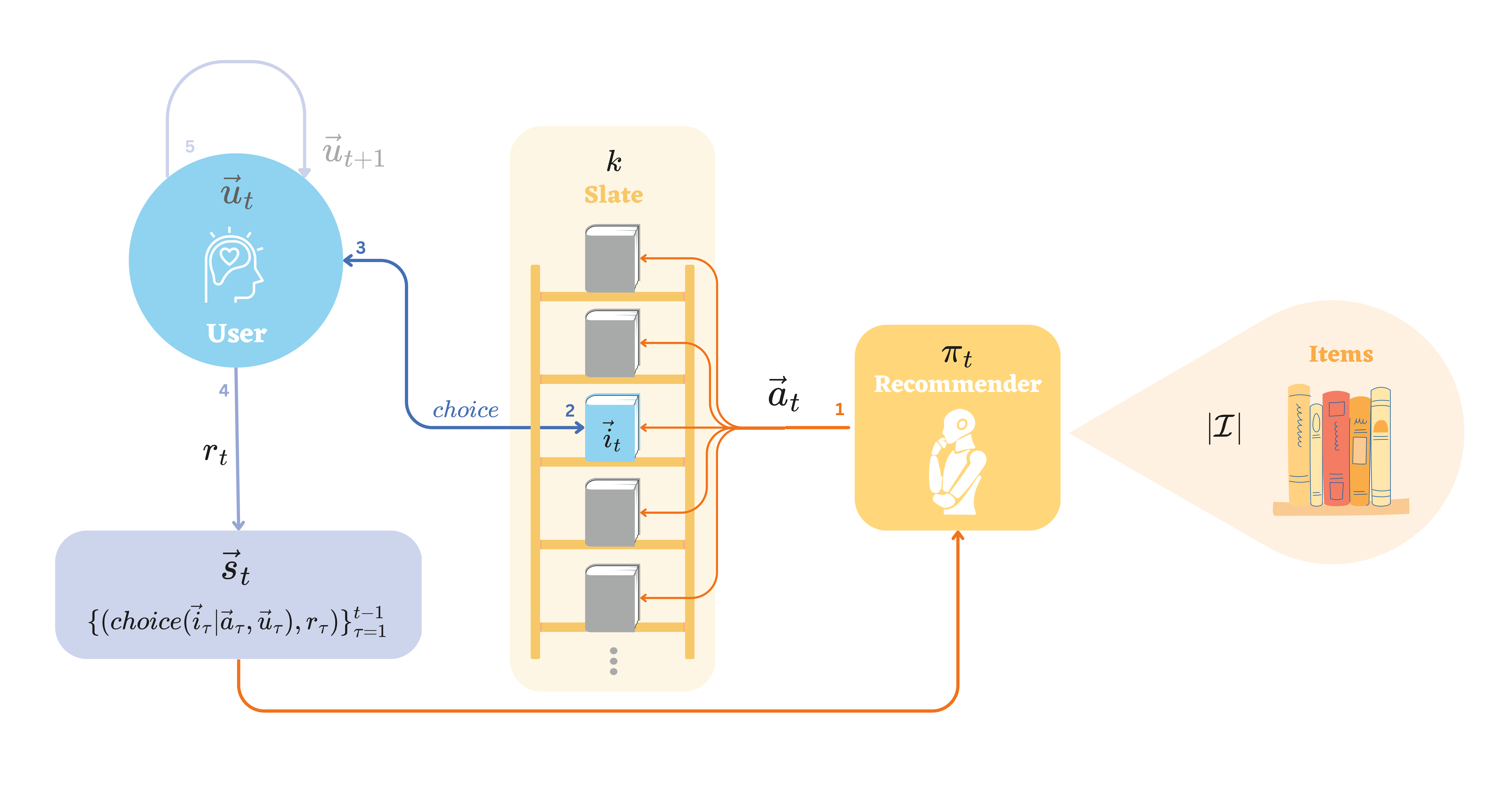
We consider an episodic MDP for slate-based recommendations. In which, a recommender presents a slate to a user, and the user selects zero or one item to consume. Then, the user respond to this consumed item with an engagement measure. The above setup is commonly used and easily extensible to real world applications (Ie et al., 2019).
Under our setup, the states can reflect the ground-truth user states , which includes static user features (such as demographics), as well as dynamic user features (such as moods). Particularly, the user history interacting with past recommendations plays a key role. This history summarization is usually domain specific, and can capture the user latent state in a partially observable MDP. The state should be predictive of immediate user response (e.g., immediate engagement, hence reward) and self-predictive (i.e., summarizes user history in a way that renders the implied dynamics Markovian).
The action space is the set of all possible recommendation slates. We assume a fixed set of items to recommend. Then, an action is a subsets , and , where is the slate size. We assume no constraints, so that each item and each slate can be recommended at each state . Note that we do not account for positional bias within a slate in this work. However, we do note that the effects of ordering within one slate can be learned using offline methods (Schnabel et al., 2016). Because a user may select no item from a slate, we assume that every slate includes a -th null item. This is standard in most choice modeling work for specifying the necessary user behaviors induced by a choice from the slate.
The transition represents the probability of user transitioning to from when action is taken by the recommender. The uncertainty mainly reflects two aspects of a recommender system MDP. First, it indicates how a user will consume a particular recommended item from the slate, marking the critical role that choice models play in evaluating the quality of a slate. Second, the user state would dynamically transit based on the consumed item. Since the ground truth is unknown, we need to learn it by interacting with environments in an online manner or utilizing offline data at hand.
The reward usually measures user engagement under state when recommended with slate . Note that, expectation is more often used to account for the uncertainty introduced by user choice. Without loss of generality, we assume trajectory reward is normalized, i.e., for any trajectory , we have . We assume that is known. This assumption largely relies on the success of existing myopic, item-level recommender (Covington et al., 2016).
The discounted factor and initial distribution are also known.
Our goal is to learn a policy which maps from state to distribution over actions (i.e., recommended slates). We use the following notations. Under some probability transition , the value function to represent the expected total discounted reward of under starting at . Similarly, we define the state-action function . Then, the expected total discounted reward of a policy under transition and reward is denoted by . We define the state-action discounted occupancy distribution , where is the probability of visiting at time step under and . The state visitation as Finally, given a vector , , , and where are constants.
We focus on low-rank MDP defined as follows, with normalized function classes.
Definition 2.1.
(Low-rank MDP) A transition model admits a low-rank decomposition with rank if there exist two embedding functions and such that
where for all and for any function , . An MDP is low-rank if admits low-rank decomposition.
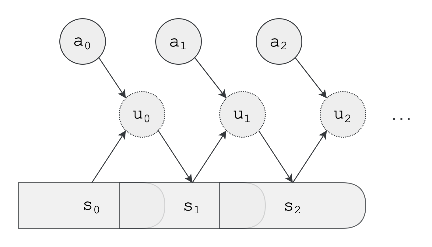
Within the context of recommender systems, low-rank MDPs capture the latent user representation dynamics as shown in Figure 2. As states are observed and follow Markovian transition, they mainly contain information of the history of user interactions with the recommender. Note that the states are likely to have overlapping information under this definition, and this simplifies the model class of as we will later discuss in Definition 2.1. The actions are the slates presented to the user at each time step. Thus, from a logged history of user and a current slate recommendation, maps to the latent representation of user. In reality, the latent space would be a compact representation space that contains the most important information that impacts user decisions. Learning such representation and interpreting would be meaningful in real life applications.
In episodic online learning, the goal is to learn a stationary policy that maximize , where is the ground truth transition. We can only reset at initial distribution , which emphasize the restricted nature of recommender systems and the challenge for exploration. The sampling of state from visitation is done by following the roll-in procedure: from starting state , at every time step , with probability we terminate, otherwise we execute and transit to .
Function approximation for representation learning. Since and are unknown, we use function classes to capture them. These model classes can be learned using the existing myopic methods for user behavior prediction.
Assumption 2.2.
(Realizability) We assume to have access to model classes and .
We assume the function approximators also follow the normalization as and , i.e., for any and , for all , for all , and for all .
We learn the functions via supervised learning oracle, which should be computationally efficient given the task.
Definition 2.3.
(Maximum Likelihood Estimator) The MLE oracle takes a dataset of tuples, and returns
The assumption above is achievable by the myopic estimators of user behavior models within recommendation context.
User choice model.
We introduce an assumption that is developed to reasonably structuralize the user behavior, and lead to effective reduction on the action space (Ie et al., 2019).
Assumption 2.4.
(Reward / transition dependence on selection) We assume that and depend only on the item on slate that is consumed by the user (including the null item).
The original action space under our MDP is with unordered -sets over . With large item space, effective exploration is impossible. Luckily, the nature of human preference and structure of recommender systems poses the possibility for reduction. With the prior assumption on user choice setup, where user select zero (null) or one item from slate, we formalize the properties as follows:
Now, notice that the transition can be described as , where represents the user’s choice on item given a slate, and is the user state transition when is consumed. This helps us to redefine uniform action in Section 3 and obtain complexity bound independent of the combinatorial action space.
Similar to the reward , we assume the user choice given a -pair is known, relying on the success of existing myopic, item-level recommender (Covington et al., 2016). Thus, the low-rank MDP realizability assumption here is used to describe .
3 Main results
We now define uniform action within the above setup. Remind that the uniform action is used to encourage user transition to some novel states. As user transition is only dependent on consumed item , we use the following definition for sufficient exploration.
Definition 3.1.
The uniform action for a slate recommendation is defined as the following:
-
1.
randomly pick an item from .
-
2.
fill the remainder of the slates using the items least-likely be selected by the user.
We further show that under this definition, the effective uniform action space is .
Lemma 3.2.
The user choose the selected item with probability at least .
We use the basic properties of probability and pigeonhole principle to further arrive at the proposition.
Proposition 3.3.
Efficient exploration action space is achieved in .
Proof.
By product rule of probability, the user select an item with probability at least under the uniform action as defined above.
By pigeonhole principle, every uniform actions lead to at least one duplicate action in this space. ∎
Note that the above change in distribution of action space definition is introduced by asymmetry of uniform distributions. More specifically, by the principle of indifference, we choose our objective on user state transition instead of naive action space (White, 2010).
3.1 Algorithm
The algorithm is based on Rep-UCB (Uehara et al., 2021), with specified definition on state space , action space , the data collection process, and the uniform action under the context of recommender system.
A state consist of static user features and a history of past recommendations and user responses. An action provides a slate recommendation. During the data collection process, for every iteration, we do one rollout under current policy . We assume the states sampled from the initial distribution follows the prior 2.2 on model classes. The sampling procedure for begins with . At every time step , we terminate with probability , or execute and observe . We sample uniform action defined by Definition 3.1. It means the recommender would do recommendations based on planning until termination, then do two uniform recommendations by the end of data collection process. We collect the tuple and update datasets.
Representation learning, building the empirical covariance matrix, and calculating the bonus are done sequentially after datasets updates. The final step within the episode is planning using the learned estimation of transition with added exploration bonus.
3.2 Analysis
The PAC bound for Rep-UCB (Uehara et al., 2021) provides us a good starting point. Our anlaysis focuses on reducing the naive combinatorial action space to be polynomial in slate size and item space size .
Theorem 3.4.
(PAC Bound for Rep-UCB-Rec) Fix , Let be a uniform mixture of and be optimal policy. Set the parameters as follows:
with probability at least , we have
The number of collected samples is at most
where
and
Proof.
The upper bound dependency on is introduced by the importance weighing of the policy to uniform action, where . Under our definition of under slate recommendation context, we naturally change the upper bound to . Note that this dependency is then interchangeable throughout the proof. ∎
4 Simulations
We discuss the simulation environment setup and the algorithm construction in this section. The simulation uses Recsim NG (Mladenov et al., 2021). A graph illustration is shown in Appendix A.
4.1 Simulation environment
Item class. A static set of items are sampled at the beginning of the simulation. Each item is represented by a -dimensional vector , where each dimension represents a topic. Each item has a length (e.g. length of a video, music or an article), and a quality that is unobserved from the user.
User interest. Users have various degrees of interests in each topics. Each user is represented by an interest vector . The user interest towards a certain item is calculated by inner product . The user interest vector and the mechanism of user interest towards items are unobserved to recommenders.
User choice. Given a slate of items, a user choose to consume one item from the slate with
This choice model is called multinomial logit model (Louviere et al., 2000). For the null item (no choice), the item is simply represented by a -dimensional zeros vector with length and quality zeros.
User dynamics. The internal transition of user interest vector allows the environment to capture Markovian transition and allow RL methods to do meaningful planning. After the consumption on item at time step , a user follows
where The constants are for normalization. Under this update, the user transits to favor the topics in more if the quality of is positive.
Reward. The reward is reflected by the user consumption time of a chosen item . It is linear with respect to the length and the user interest of item .
4.2 Algorithm construction
The state is a history of length that the user interacts with the recommender. The history contains the slate recommendations and user responses at each time step . We construct the sampling procedure introduced by At each episode, the recommender follows the current learned policy and observe user responses. Until the rollin procedure terminates, the recommender further does two step uniform recommendation. The supervised learning for representation is done in an offline manner, where we combine two model classes and train them together to make predictions from to . Note that by definiton of states, we only predict the user next response towards current action, and slide up one time step the time window of history. It eases the complexity of large state space to and reflects on the special structure behind recommender systems. After calculating the emperical covariance matrix and exploration bonus, we utilize a costomized simulator where transition and reward are estimated. Standard policy gradient methods are used to calculate the updated policy within the this environment under and .
5 Conclusion
In this work, we propose a sample-efficient representation learning algorithm, using the standard slate recommendation setup, to treat this as an online RL problem with low-rank Markov decision processes (MDPs). We show that the sample complexity for learning near-optimal policy is where is the slate size and is the item space. We further show the detailed construction of a recommender simulation environment with the proposed setup and sampling method.
References
- Afsar et al. (2022) Afsar, M. M., Crump, T., and Far, B. Reinforcement learning based recommender systems: A survey. ACM Computing Surveys, 55(7):1–38, 2022.
- Agarwal et al. (2020) Agarwal, A., Kakade, S., Krishnamurthy, A., and Sun, W. Flambe: Structural complexity and representation learning of low rank mdps. Advances in neural information processing systems, 33:20095–20107, 2020.
- Breese et al. (2013) Breese, J. S., Heckerman, D., and Kadie, C. Empirical analysis of predictive algorithms for collaborative filtering. arXiv preprint arXiv:1301.7363, 2013.
- Chen et al. (2021) Chen, M., Chang, B., Xu, C., and Chi, E. H. User response models to improve a reinforce recommender system. In Proceedings of the 14th ACM International Conference on Web Search and Data Mining, pp. 121–129, 2021.
- Covington et al. (2016) Covington, P., Adams, J., and Sargin, E. Deep neural networks for youtube recommendations. In Proceedings of the 10th ACM conference on recommender systems, pp. 191–198, 2016.
- Deshpande & Karypis (2004) Deshpande, M. and Karypis, G. Item-based top-n recommendation algorithms. ACM Transactions on Information Systems (TOIS), 22(1):143–177, 2004.
- Efroni et al. (2022) Efroni, Y., Jin, C., Krishnamurthy, A., and Miryoosefi, S. Provable reinforcement learning with a short-term memory. In International Conference on Machine Learning, pp. 5832–5850. PMLR, 2022.
- Gauci et al. (2018) Gauci, J., Conti, E., Liang, Y., Virochsiri, K., He, Y., Kaden, Z., Narayanan, V., Ye, X., Chen, Z., and Fujimoto, S. Horizon: Facebook’s open source applied reinforcement learning platform. arXiv preprint arXiv:1811.00260, 2018.
- Gomez-Uribe & Hunt (2015) Gomez-Uribe, C. A. and Hunt, N. The netflix recommender system: Algorithms, business value, and innovation. ACM Transactions on Management Information Systems (TMIS), 6(4):1–19, 2015.
- He & McAuley (2016) He, R. and McAuley, J. Fusing similarity models with markov chains for sparse sequential recommendation. In 2016 IEEE 16th international conference on data mining (ICDM), pp. 191–200. IEEE, 2016.
- Ie et al. (2019) Ie, E., Jain, V., Wang, J., Narvekar, S., Agarwal, R., Wu, R., Cheng, H.-T., Lustman, M., Gatto, V., Covington, P., et al. Reinforcement learning for slate-based recommender systems: A tractable decomposition and practical methodology. arXiv preprint arXiv:1905.12767, 2019.
- Jacobson et al. (2016) Jacobson, K., Murali, V., Newett, E., Whitman, B., and Yon, R. Music personalization at spotify. In Proceedings of the 10th ACM Conference on Recommender Systems, pp. 373–373, 2016.
- Jin et al. (2020) Jin, C., Yang, Z., Wang, Z., and Jordan, M. I. Provably efficient reinforcement learning with linear function approximation. In Conference on Learning Theory, pp. 2137–2143. PMLR, 2020.
- Joachims (2002) Joachims, T. Optimizing search engines using clickthrough data. In Proceedings of the eighth ACM SIGKDD international conference on Knowledge discovery and data mining, pp. 133–142, 2002.
- Konstan et al. (1997) Konstan, J. A., Miller, B. N., Maltz, D., Herlocker, J. L., Gordon, L. R., and Riedl, J. Grouplens: Applying collaborative filtering to usenet news. Communications of the ACM, 40(3):77–87, 1997.
- Koren et al. (2009) Koren, Y., Bell, R., and Volinsky, C. Matrix factorization techniques for recommender systems. Computer, 42(8):30–37, 2009.
- Krestel et al. (2009) Krestel, R., Fankhauser, P., and Nejdl, W. Latent dirichlet allocation for tag recommendation. In Proceedings of the third ACM conference on Recommender systems, pp. 61–68, 2009.
- Liu et al. (2020) Liu, F., Guo, H., Li, X., Tang, R., Ye, Y., and He, X. End-to-end deep reinforcement learning based recommendation with supervised embedding. In Proceedings of the 13th International Conference on Web Search and Data Mining, pp. 384–392, 2020.
- Louviere et al. (2000) Louviere, J. J., Hensher, D. A., and Swait, J. D. Stated choice methods: analysis and applications. Cambridge university press, 2000.
- Luce (2012) Luce, R. D. Individual choice behavior: A theoretical analysis. Courier Corporation, 2012.
- Mehrotra et al. (2019) Mehrotra, R., Lalmas, M., Kenney, D., Lim-Meng, T., and Hashemian, G. Jointly leveraging intent and interaction signals to predict user satisfaction with slate recommendations. In The World Wide Web Conference, pp. 1256–1267, 2019.
- Misra et al. (2020) Misra, D., Henaff, M., Krishnamurthy, A., and Langford, J. Kinematic state abstraction and provably efficient rich-observation reinforcement learning. In International conference on machine learning, pp. 6961–6971. PMLR, 2020.
- Mladenov et al. (2021) Mladenov, M., Hsu, C.-W., Jain, V., Ie, E., Colby, C., Mayoraz, N., Pham, H., Tran, D., Vendrov, I., and Boutilier, C. Recsim ng: Toward principled uncertainty modeling for recommender ecosystems. arXiv preprint arXiv:2103.08057, 2021.
- Mnih & Salakhutdinov (2007) Mnih, A. and Salakhutdinov, R. R. Probabilistic matrix factorization. Advances in neural information processing systems, 20, 2007.
- Moshfeghi et al. (2011) Moshfeghi, Y., Piwowarski, B., and Jose, J. M. Handling data sparsity in collaborative filtering using emotion and semantic based features. In Proceedings of the 34th international ACM SIGIR conference on Research and development in Information Retrieval, pp. 625–634, 2011.
- Rendle et al. (2010) Rendle, S., Freudenthaler, C., and Schmidt-Thieme, L. Factorizing personalized markov chains for next-basket recommendation. In Proceedings of the 19th international conference on World wide web, pp. 811–820, 2010.
- Schnabel et al. (2016) Schnabel, T., Swaminathan, A., Singh, A., Chandak, N., and Joachims, T. Recommendations as treatments: Debiasing learning and evaluation. In international conference on machine learning, pp. 1670–1679. PMLR, 2016.
- Shani et al. (2005) Shani, G., Heckerman, D., Brafman, R. I., and Boutilier, C. An mdp-based recommender system. Journal of Machine Learning Research, 6(9), 2005.
- Srebro et al. (2004) Srebro, N., Rennie, J., and Jaakkola, T. Maximum-margin matrix factorization. Advances in neural information processing systems, 17, 2004.
- Swaminathan et al. (2017) Swaminathan, A., Krishnamurthy, A., Agarwal, A., Dudik, M., Langford, J., Jose, D., and Zitouni, I. Off-policy evaluation for slate recommendation. Advances in Neural Information Processing Systems, 30, 2017.
- Uehara et al. (2021) Uehara, M., Zhang, X., and Sun, W. Representation learning for online and offline rl in low-rank mdps. arXiv preprint arXiv:2110.04652, 2021.
- Van den Oord et al. (2013) Van den Oord, A., Dieleman, S., and Schrauwen, B. Deep content-based music recommendation. Advances in neural information processing systems, 26, 2013.
- Van Meteren & Van Someren (2000) Van Meteren, R. and Van Someren, M. Using content-based filtering for recommendation. In Proceedings of the machine learning in the new information age: MLnet/ECML2000 workshop, volume 30, pp. 47–56. Barcelona, 2000.
- Viappiani & Boutilier (2010) Viappiani, P. and Boutilier, C. Optimal bayesian recommendation sets and myopically optimal choice query sets. Advances in neural information processing systems, 23, 2010.
- White (2010) White, R. Evidential symmetry and mushy credence. 2010.
- Xin et al. (2020) Xin, X., Karatzoglou, A., Arapakis, I., and Jose, J. M. Self-supervised reinforcement learning for recommender systems. In Proceedings of the 43rd International ACM SIGIR conference on research and development in Information Retrieval, pp. 931–940, 2020.
- Zhou et al. (2020) Zhou, K., Wang, H., Zhao, W. X., Zhu, Y., Wang, S., Zhang, F., Wang, Z., and Wen, J.-R. S3-rec: Self-supervised learning for sequential recommendation with mutual information maximization. In Proceedings of the 29th ACM international conference on information & knowledge management, pp. 1893–1902, 2020.
Appendix A Graph illustration of the simulation environment.