The IA Guide:
A Breakdown of Intrinsic Alignment Formalisms

Abstract

We summarize common notations and concepts in the field of Intrinsic Alignments (IA). IA refers to physical correlations involving galaxy shapes, galaxy spins, and the underlying cosmic web. Its characterization is an important aspect of modern cosmology, particularly in weak lensing analyses. This resource is both a reference for those already familiar with IA and designed to introduce someone to the field by drawing from various studies and presenting a collection of IA formalisms, estimators, modeling approaches, alternative notations, and useful references.

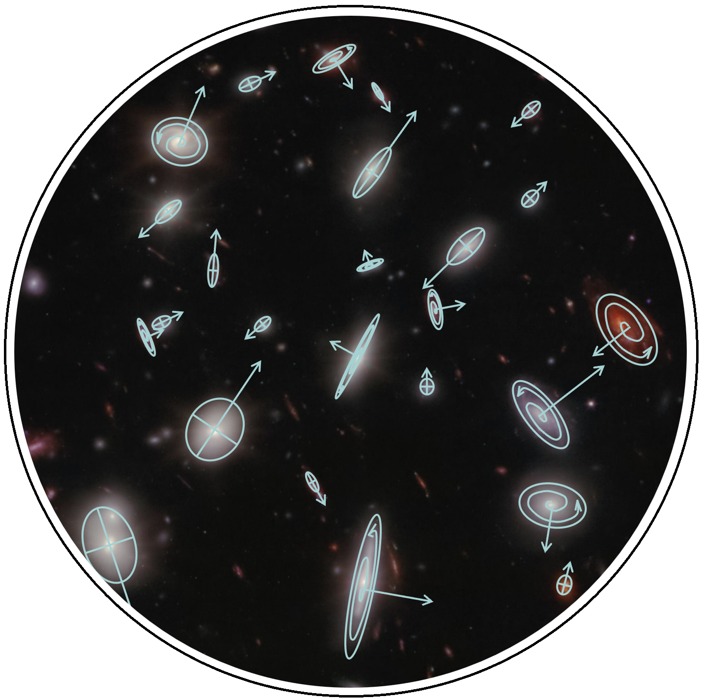
Figure 1: Galaxy shapes and orientations traced over a portion of JWST’s NIRCam image of Abell 2744.

1 Introduction

This resource is a condensed overview of quantities relevant for describing the intrinsic alignment (IA) of galaxies. For scientists new to the field, it is a useful starting place which contains a broad introduction to IA and helpful references with more details and derivations. It is also structured to be a quick reference for those already familiar with IA. This is not a review article and not necessarily intended to be read beginning-to-end. Sections 2-7 each contain common formalisms of an IA estimator, brief pedagogical explanations with practical advice, alternative notations, and useful references. The remaining sections summarize IA modeling and applications. Terms in teal are hyperlinked to glossary entries at the end of the document.

IA refers to correlations between galaxy shapes and between galaxy shapes and the underlying dark matter distribution. These arise naturally within our current understanding of galaxy formation, as confirmed by hydrodynamic simulations (Kiessling et al., 2015; Bhowmick et al., 2020; Samuroff et al., 2021). In the case of elliptical galaxies, shapes are elongated along the external gravitational field (Croft & Metzler, 2000; Catelan et al., 2001). The shapes of spiral galaxies are typically associated with their angular momentum, which arises from the torque produced by the external gravitational field (Heavens et al., 2000; Codis et al., 2015). The alignments of spiral galaxy shapes are much weaker than for ellipticals and so far have not been directly observed (Zjupa et al., 2020; Johnston et al., 2019; Samuroff et al., 2022). Some studies use galaxy spin instead of shapes to measure alignment (Lee, 2011), though here we focus on shapes as they can be more directly connected to cosmic shear and are most commonly used in observational studies. Lee & Erdogdu (2007) provides a pedagogical overview of the physics and formalisms of spin alignments.

While IA can be used as a cosmological probe, historically it is most often studied as a contaminant of weak lensing. As light travels to us from distant galaxies, it is bent by the gravitational field of the large-scale structure of the Universe and thus we observe distorted galaxy images. When this effect is too small to be detected for individual galaxies, we say that we are in the weak lensing regime. The resulting shear in these galaxy shapes is known as cosmic shear, and is a primary tool used to probe cosmological parameters (Refregier, 2003). The correlations between observed galaxy shapes used to measure weak lensing are difficult to separate from those that arise from IA. Studies show that IA can account for a 30% error on the matter power spectrum amplitude as measured by cosmic shear (Hirata et al., 2007), making IA one of the most significant sources of systematic errors in weak lensing measurements.

Additional note: galaxy types

Throughout this guide, we refer to galaxies as “early-type” or “late-type”, “blue” or “red”, and “elliptical” or “spiral”, depending on the reference we are following. Early-type galaxies are usually elliptical or lenticular and tend to be redder in color. Late-type galaxies are spiral and typically blue. The terminology “early” and “late” does not refer to the age of the galaxy, but to their ordering in the Hubble Sequence (also known as “The Tuning Fork”) when Hubble initially thought that ellipticals evolve into spirals (Hubble, 1926). Although sometimes used interchangeably, it’s important to keep in mind that populations may be defined differently in different analyses.

1.1 Reviews

Here is a list of available reviews and primers on IA. A Zotero group of key IA papers can be found below.

• “The intrinsic alignment of galaxies and its impact on weak gravitational lensing in an era of precision cosmology” Troxel & Ishak (2015)
  The first comprehensive review on intrinsic alignments, presenting extensive documentation of commonly used formalisms and the role of IA in precision cosmology.

• “Galaxy alignments: An overview” Joachimi et al. (2015)
  Broad synopsis of IA, including physical motivations, a historical overview, and main trends.

• “Galaxy alignments: Observations and impact on cosmology” Kirk et al. (2015)
  Descriptions of formalisms for measuring shapes and IA tracer s, overview of IA observations, and discussion of cosmological impacts and mitigation.

• “Galaxy alignments: Theory, modelling and simulations” Kiessling et al. (2015)
  Detailed overview of common models and IA in $N$-body and hydrodynamic simulations.

2 Ellipticity

IA studies model simulated, three-dimensional (3D) galaxy shapes as triaxial ellipsoids, and observed galaxies as their projected shape on the sky: two-dimensional (2D) ellipses. This 2D ellipticity is quantified in terms of the lengths of the major and minor axes of the ellipse ($a$ and $b$, respectively, with $b\leq a$) and the orientation angle of the major axis, $\theta$, as shown in Figure 2.

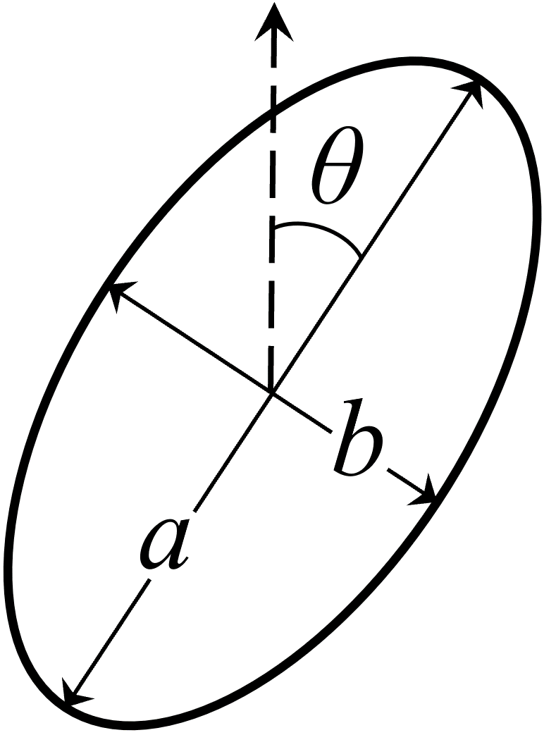
Figure 2: The quantities $a$, $b$ and $\theta$ which define the shape and orientation of an ellipse.

For the detection of IA, ellipticity is typically measured relative to directions tracing the tidal field (e.g., positions of galaxy overdensities in real data, or reconstructed tidal fields in simulations), often as a function of transverse separation $r_{p}$. By convention, the alignment signal is highest for very elongated shapes (larger axis ratio) that point along the direction of the tidal field.

While the formalisms below are standard, the methods of fitting shapes to observations vary across surveys and can impact the resulting IA signal. The signal is also correlated with the clustering of the galaxy sample and depends on how far along the Line of Sight (LOS) the measurement is averaged over. Therefore, it is more common to use IA correlation function s rather than a relative ellipticity, although ellipticity is a component of most estimator s.

2.1 Ellipticity: 2D Formalism

There are two different ways in which the ellipticity of 2D shapes is commonly quantified. We will refer to these as $\varepsilon$ and $\chi$ and to ellipticity generically as $\epsilon$. In the rest of the document $\epsilon$ can be taken to stand for either of the two ellipticity definitions. These are defined as:

$$\varepsilon=\frac{a-b}{a+b}\exp(2\mathrm{i}\theta)\,$$ (6)

$$\chi=\frac{a^{2}-b^{2}}{a^{2}+b^{2}}\exp(2\mathrm{i}\theta)\,.$$ (7)

Both quantities are often referred to as the ellipticity, but $\chi$ is also known as the distortion (Mandelbaum et al., 2014) or the normalized polarization (Viola et al., 2014). The definition $\varepsilon$ (but usually denoted $\epsilon$) is often used in weak lensing studies because it is an unbiased estimator of the cosmic shear, $\gamma$. Whereas $\chi$ must be adjusted by the responsivity $\mathcal{R}$ which quantifies the response of the ellipticity to an applied gravitational shear:

$$\gamma=\frac{\langle\chi\rangle}{2\mathcal{R}}\,.$$ (8)

$\mathcal{R}=1-\chi_{\mathrm{rms}}$ (rms is the root mean square) and is typically $\approx 0.9$ depending on the galaxy sample (Singh & Mandelbaum, 2016). In later parts of this guide, $\epsilon$ is used generally. It is assumed that where the $\chi$ definition is intended, it will have been adjusted for the responsivity so $\mathcal{R}$ is not explicitly shown.

Ellipticity is a complex quantity which can be broken up into its real and imaginary components, $\epsilon_{1}$ and $\epsilon_{2}$:

$$\epsilon=\epsilon_{1}+\mathrm{i}\epsilon_{2}\,,$$ (9)

where

$$\epsilon_{1} =\lvert\epsilon\rvert\cos(2\theta)$$ (10)

$$\epsilon_{2} =\lvert\epsilon\rvert\sin(2\theta)\,.$$ (11)

The factor of 2 arises because ellipticity is a spin-2 quantity, which means that it is invariant under rotations of integer multiples of $\pi$ (not $2\pi$). See Figure 3. The angle $\theta$ is usually defined as East of North. Its range can be $0-\pi$ or $\pm\frac{\pi}{2}$.

$\epsilon_{1}$ represents the orientation of an ellipse relative to the direction where $\theta=0$ and $\epsilon_{2}$ represents the orientation relative to the direction where $\theta=\frac{\pi}{4}$. Note that $\epsilon_{1}$ and $\epsilon_{2}$ contain the same information (Figure 3). When measured relative to another galaxy or the direction of the tidal field, they are usually denoted as $\epsilon_{+}$ and $\epsilon_{\times}$, with the subscripts respectfully read as “plus” and “cross”. $\epsilon_{+}>0$ indicates an alignment along the tidal field direction, and $\epsilon_{+}<0$ indicates a tangential orientation as seen in gravitational shear (Section 3). $\epsilon_{\times}$ is equivalent to $\epsilon_{2}$. On average, $\epsilon_{\times}$ is 0 in the real Universe.

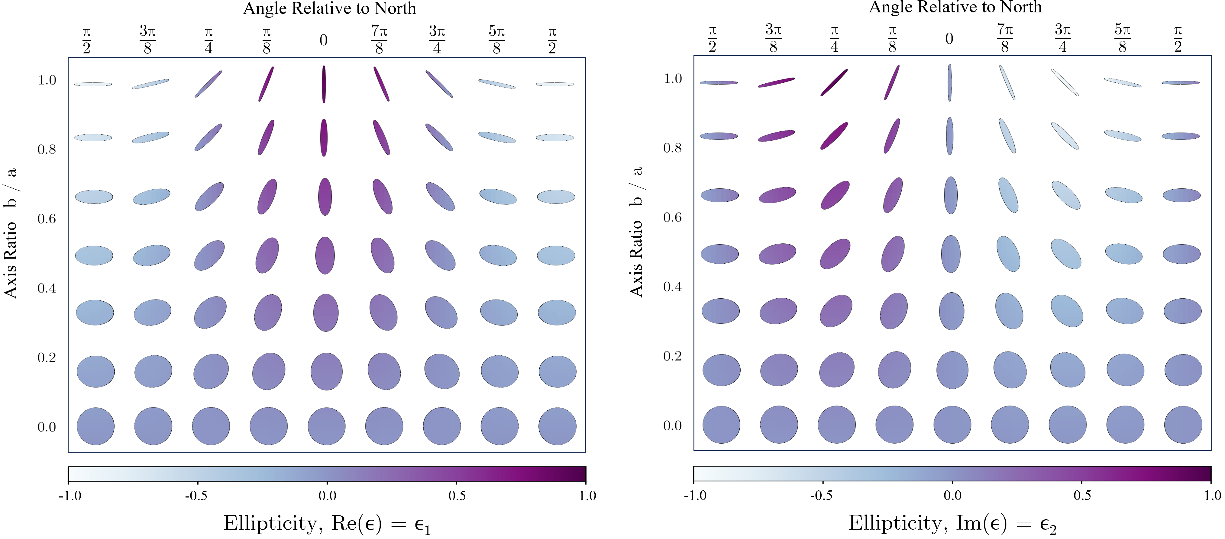
Figure 3: Visualization of the real and imaginary components of ellipticity, as described in Section 2. These functionally contain the same information. $\epsilon_{1}$ is maximum when a shape is highly elongated and exactly aligned with the angle that the ellipticity is defined relative to, most commonly North. $\epsilon_{2}$ is maximum when the shape is aligned with $\pi/4$ away from the principal angle.

2.2 Ellipticity: Modeling and 3D Formalism

Ellipticity from particles
Simulated galaxies and halos are usually modeled as triaxial ellipsoids composed of “particles”. To summarize the shape of these objects, it’s common to use the inertia tensor, I, which is computed by summing over the positions $i,j\in(x,y,z)$ of $N$ particles. To better approximate the object’s position and shape, this sum is usually weighted by particle mass or luminosity (when applicable). For weights $w_{k}$ which sum to $W$, this form of the moment of inertia tensor is (Samuroff et al., 2021)

$$I_{ij}=\frac{1}{W}\sum^{N}_{k=1}w^{k}x_{i}^{k}x_{j}^{k}\,.$$ (12)

It’s also common to weight $I_{ij}$ by distance from the center of the object. This center-weighting produces the reduced inertia tensor (Chisari et al., 2015),

$$\tilde{I}_{ij}=\frac{1}{W}\sum^{N}_{k=1}w^{k}\frac{x_{i}^{k}x_{j}^{k}}{x^{l}x_{l}}\,.$$ (13)

Note that $l$ are dummy indices that are contracted over for summation. As a result, the denominator of the above fraction represents the distance of particle $k$ from the object’s center of mass. The reduced inertia tensor can provide a better approximation of the shape of the object at its center (Joachimi et al., 2013). In Eqs. (12) and (13), the weighting kernel is inherently round, and thus produces a bias in the estimator s. To avoid this limitation, studies often iteratively rescale the lengths of the ellipse axes while keeping the volume constant. (Mandelbaum et al., 2015; Schneider et al., 2012; Tenneti et al., 2014).

An ellipsoid can be constructed using the eigenvectors and eigenvalues of $I_{ij}$, which can then be projected along the $z$-axis into its 2D second moments $Q_{11}$, $Q_{22}$, $Q_{12}+Q_{21}$ (Bartelmann & Schneider, 2001).

The projected ellipticity $\chi$ is obtained via

$$\chi=\frac{(Q_{11}-Q_{22},2Q_{12})}{Q_{11}+Q_{22}+2\sqrt{\det\mathbf{Q}}}\,.$$ (14)

Note that the denominator is different if the alternative definition of ellipticity is used - see Section 2.1 and Mandelbaum et al. (2014).

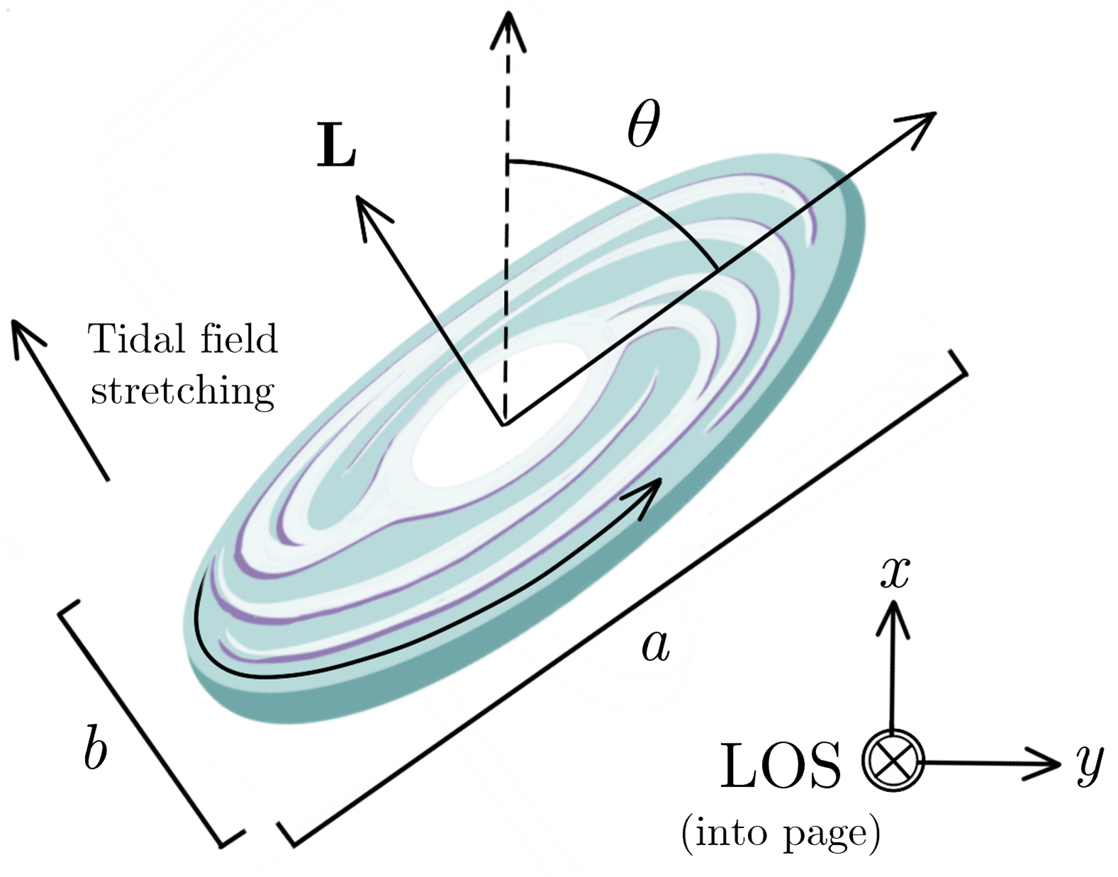
Figure 4: The set up for obtaining the projected shape of a spiral galaxy. In linear theory, the angular momentum vector $\mathbf{L}$ of the galaxy is aligned along the direction of tidal stretching. The projected axis ratio, $b/a$, is a function of $\mathbf{L}$ and the ratio of the disk’s intrinsic thickness to its diameter (not shown here).

Projected Ellipticity from angular momentum
Late-type galaxies are typically modeled as circular discs and their ellipticity is often assumed to be aligned with their angular momentum vector (tidal torquing or spin alignment), $\mathbf{L}=L_{i}=\left\{L_{x},L_{y},L_{\parallel}\right\}^{\tau}$. $\tau$ denotes the transpose vector and $i={1,2,3}$ the three spatial directions (Figure 4). To obtain the projected shape of a spiral galaxy along the LOS, or $L_{\parallel}$, the orientation angle $\theta$ is given by:

$$\theta=\frac{\pi}{2}+\text{arctan}\left(\frac{L_{y}}{L_{x}}\right)\,,$$ (15)

and the axis ratio:

$$\frac{b}{a}=\frac{\lvert L_{\parallel}\lvert}{\lvert\mathbf{L}\lvert}+r_{\text{edge-on}}\sqrt{1-\frac{L_{\parallel}^{2}}{\lvert\mathbf{L}\rvert^{2}}}\,.$$ (16)

$r_{\text{edge-on}}$ describes the ratio of the disc thickness to disc diameter, which is approximately equivalent to the axis ratio for a galaxy viewed edge-on; this contribution is expected to be significant for galaxies with bulges (Joachimi et al., 2013). Assuming linear tidal torquing, a halo’s spin is written as (Lee & Pen, 2008)

$$L_{i}\propto\epsilon_{ijk}I^{k}_{l}T^{jl}\,,$$ (17)

where ${i,j,k}={1,2,3}$ in the three spatial directions, $\epsilon_{ijk}$ the Levi-Civita symbol and $T^{jl}$ the gravitational tidal shear. The latter, which is a symmetric tensor, is defined as (e.g. Blazek et al., 2011)

$$T_{ij}=\frac{\partial^{2}\Phi}{\partial x_{i}\partial x_{j}}\,,$$ (18)

where $\Phi$ is the gravitational potential, $x$ represents comoving Cartesian coordinates and the indices $\{i,j\}=\{1,2,3\}$ indicate the three spatial directions. Following Eq. (17), tidal torquing leads to quadratic alignments of galaxy shapes with the tidal shear.

Ellipticity from tidal field
Early-type galaxies are considered to be triaxial ellipsoids whose axes align with the underlying gravitational tidal shear, $T_{ij}$ (Catelan et al., 2001). In order to derive the predicted galaxy ellipticities given $T_{ij}$, we can project the 3D tidal field along two axes at the location of each galaxy. The convention is to project along the galaxy’s North Pole distance, $\phi_{1}$, and right ascension, $\phi_{2}$ (see 5). The latter is the angle complementary to declination. In this setting, $\epsilon_{1}>0$ corresponds to east-west elongation and $\epsilon_{2}>0$ corresponds to northeast-southwest elongation. We first consider a Cartesian orthonormal basis, $(\hat{\mathbf{x}},\hat{\mathbf{y}},\hat{\mathbf{z}})$, at the location of each galaxy. We then rotate this basis into $(\mathbf{\hat{n}},\boldsymbol{\hat{\phi}_{1}},\boldsymbol{\hat{\phi}_{2}})$, such that $\mathbf{\hat{n}}$ is parallel to the LOS to the galaxy. These two bases are related by

$$\boldsymbol{\hat{\phi}_{1}} = \cos{\phi_{1}}\cos{\phi_{2}}\,\hat{\mathbf{x}}+\cos{\phi_{1}}\sin{\phi_{2}}\,\hat{\mathbf{y}}-\sin{\phi_{1}}\,\hat{\mathbf{z}}\,,$$ (19)

$$\boldsymbol{\hat{\phi_{2}}} = -\sin{\phi_{2}}\,\hat{\mathbf{x}}+\cos{\phi_{2}}\,\hat{\mathbf{y}}.$$ (20)

The next step is to intermediately define the linear combinations,

$$m^{i}_{+} = \frac{1}{\sqrt{2}}\left(\boldsymbol{\hat{\phi}_{2}^{i}}-i\boldsymbol{\hat{\phi}_{1}^{i}}\right)$$ (21)

$$m^{i}_{-} = \frac{1}{\sqrt{2}}\left(\boldsymbol{\hat{\phi}_{2}^{i}}+i\boldsymbol{\hat{\phi}_{1}^{i}}\right)\,,$$ (22)

Having defined the above fields, we can decompose the 3D tidal shear into the rotated basis, as (Schmidt & Jeong, 2012)

$$T_{\pm}=\sum_{i=1}^{3}\sum_{j=1}^{3}{m^{i}}_{\mp}{m^{j}}_{\mp}T_{ij}\,,$$ (23)

where $T_{\pm}$ are the 2D ellipticities, such that (Tsaprazi et al., 2022)

$$\epsilon_{1}\pm i\epsilon_{2}=-\frac{C_{1}}{4\pi G}T_{\pm}\,,$$ (24)

in the nonlinear alignment model, for example, described in Section 8.3. Here $C_{1}$ is the IA amplitude (introduced in Section 8.1) and $(\epsilon_{1},\epsilon_{2})$ the observed galaxy ellipticities.

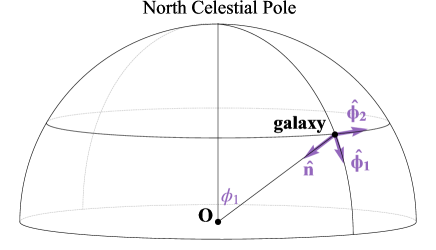
Figure 5: Representation of the Northern Celestial Hemisphere. The observer is indicated by O and a given observed galaxy by galaxy. The purple basis indicates the rotated basis defined in Eq. (19) and Eq. (20), whereas $\phi_{1}$ is the angle from the North Pole.

2.3 Ellipticity: Additional Notations

• $\epsilon$: frequently used rather than $\varepsilon$ and sometimes instead of $\chi$.

• $e$: sometimes used equivalently to $\epsilon$.

• $\epsilon_{\text{T}}$ or $\epsilon_{\text{t}}$: the tangential component of ellipticity, equivalent to $\epsilon_{+}$.

• $\eta$: sometimes used instead of $\chi$.

• $\phi$: sometimes used for the orientation angle.

• $a,b$: sometimes denote the length of the semi-axes of the ellipse, rather than the full axes lengths.

• $q$: the ratio of the ellipse axes, $b/a$, with $b\leq a$.

2.4 Ellipticity: References

• “On the intrinsic shape of elliptical galaxies” Binggeli (1980)
  Historical discussion of the true and projected shapes of elliptical galaxies.

• “Weak gravitational lensing” Bartelmann & Schneider (2001)
  Review paper, Section 4 contains additional ellipticity details.

• “Shapes and shears, stars and smears: Optimal measurements for Weak Lensing” Bernstein & Jarvis (2002)
  Defines the shear responsivity factor, $\mathcal{R}$.

• “Intrinsic galaxy shapes and alignments I: Measuring and modelling COSMOS intrinsic galaxy ellipticities” Joachimi et al. (2013)
  Contains condensed formulae for projecting 3D shapes to 2D.

• “The third gravitational lensing accuracy testing (GREAT3) challenge handbook” Mandelbaum et al. (2014)
  Section 2.1 includes different ellipticity definitions.

• “Means of confusion: How pixel noise affects shear estimates for weak gravitational lensing” (Melchior & Viola, 2012)
  Appendix A discusses pros and cons of different ellipticity definitions.

• “Intrinsic alignments of galaxies in the Illustris simulation” Hilbert et al. (2017)
  Additional notation and definitions for 3D shapes.

• “The mass dependence of dark matter halo alignments with large-scale structure” Piras et al. (2018)
  Derivations for the 3D shapes of galaxies from the moment of inertia tensor.

• “Intrinsic alignment as an RSD contaminant”, Lamman et al. (2023)
  Appendix A contains condensed relations for flat projection of a triaxial shape.

• “Galaxy shape statistics in the effective field theory” Vlah et al. (2021)
  Formalism for projecting 3D shapes in forms that are convenient for numerical implementation.

• “Intrinsic alignment from multiple shear estimates: A first application to data and forecasts for Stage IV” MacMahon & Leonard (2023)
  A demonstration of how systematic effects in determining shapes affect intrinsic alignments, in a way distinct from the weak lensing signal.

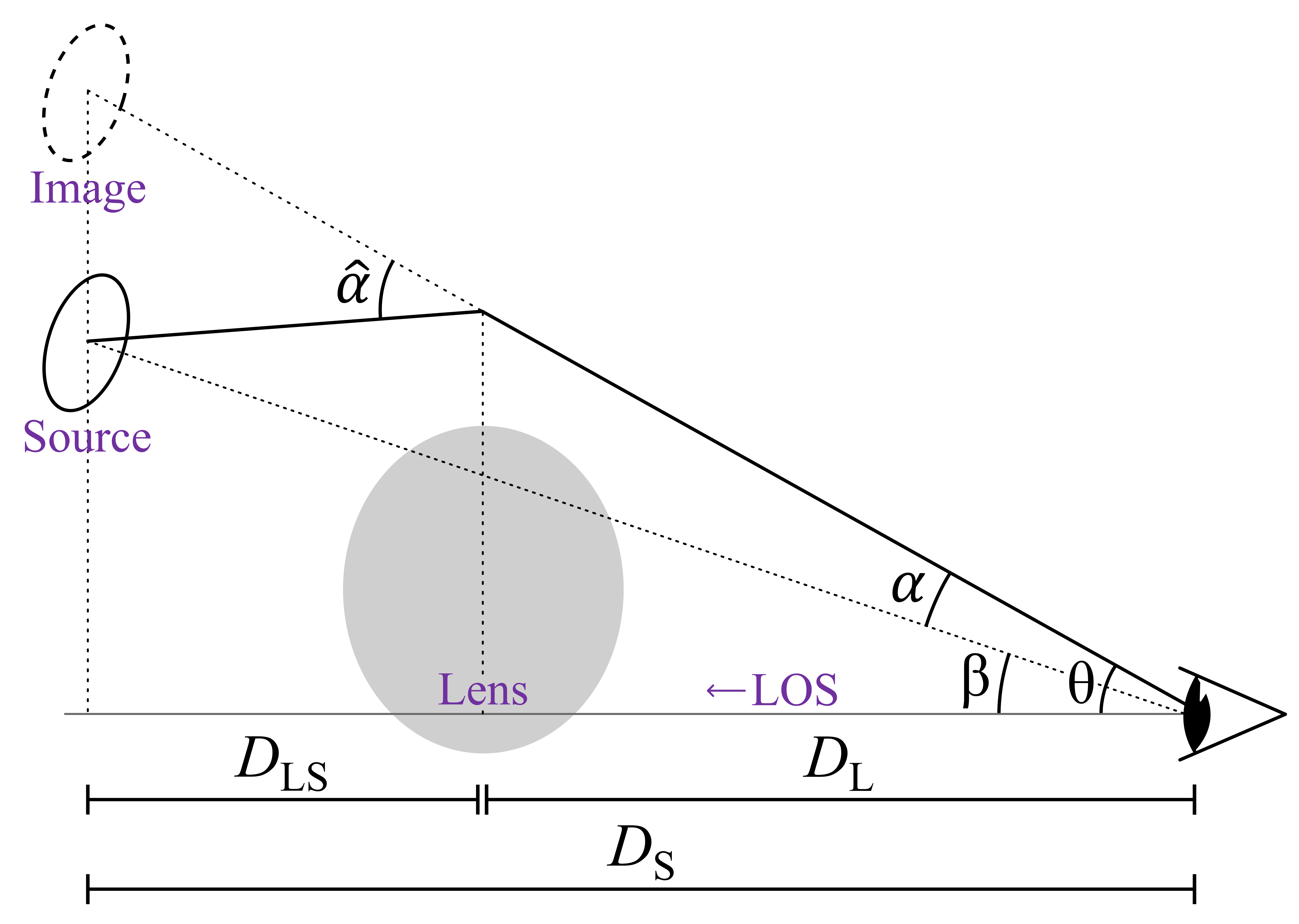
Figure 6: A diagram of a gravitational lensing system. A mass concentrated at an angular diameter distance $D_{\text{L}}$ from the observer lenses the light from a source located at distance $D_{\text{S}}$. In the thin-lens approximation, the true angular position of the light source $\boldsymbol{\beta}$ with respect to the LOS is related to the observed angular position $\boldsymbol{\theta}$ through the lens or ray-tracing equation, $\boldsymbol{\beta}=\boldsymbol{\theta}-\boldsymbol{\alpha}(\boldsymbol{\theta})$, where $\boldsymbol{\alpha}$ is the reduced deflection angle measured by the observer. The angle $\hat{\boldsymbol{\alpha}}$ is the deflection angle measured at the lens. Note that angles are exaggerated to aid visualization.

3 Shear

IA is often measured as a contaminant of cosmic shear (Bernstein & Jarvis, 2002; Hirata & Seljak, 2004) and is sometimes referred to as intrinsic shear, $\gamma_{\text{I}}$. The systematic distortion of galaxy light by foreground mass creates a tangential shear on the sky, $\gamma_{\text{lensing}}$, often acting in opposition to the signal from tidal alignment at large scales. As these two phenomena are difficult to distinguish observationally and are necessarily measured together, much of the IA formalism described in this and following sections is from weak lensing.

3.1 Shear: Formalism

The observed shear signal is the combination of the intrinsic component of shapes and the component gravitationally lensed by foreground mass:

$$\gamma_{\text{observed}}=\gamma_{\text{I}}+\gamma_{\text{lensing}}\,.$$ (25)

This mathematical sum is an approximation for when the effects are small, as in weak lensing; see the note about shear addition below. Shear quantifies the shape of galaxies and thus is related to the ellipticity described in Section 2.1. Lensing is often defined via the critical mean density, $\Sigma_{\text{crit}}$, which is the maximum surface density before the light of a source is split into multiple images by a foreground mass. $\Sigma_{\text{crit}}$ is a function of fundamental constants and the radial separations involved in the lensing system, as illustrated in Figure 6.

$$\Sigma_{\text{crit}}=\frac{c^{2}D_{\mathrm{S}}}{4\pi GD_{\mathrm{L}}D_{\mathrm{LS}}}.$$ (26)

For instance, in galaxy-galaxy lensing, as opposed to lensing by the large-scale structure, the shear is caused by a particular overdensity. It is the difference between the average surface density within some projected separation $\bar{\Sigma}(<r_{p})$, and the surface density at separation $\Sigma(r_{p})$, as a fraction of $\Sigma_{\rm crit}$:

$$\gamma_{\text{overdensity}}=\frac{\bar{\Sigma}(<r_{p})-\Sigma(r_{p})}{\Sigma_{\rm crit}}\,.$$ (27)

Variable definitions

• $\gamma$: total shear, as described in Section 4.

• $\gamma_{\mathrm{I}}$: intrinsic shear due to tidal alignment.

• $\langle\epsilon\rangle$: expectation value of the ellipticity.

• $\Sigma$: surface overdensity, projected to the plane of the sky, i.e., the mass density integrated along the LOS.

• $D_{\mathrm{S}}$: radial distance between observer and light source.

• $D_{\mathrm{L}}$: radial distance between observer and gravitational lens.

• $D_{\mathrm{LS}}$: radial distance between light source and lens.

• $c$: speed of light.

• G: gravitational constant.

3.2 Shear: Additional Notation

• $\gamma_{t}$ or $\gamma_{T}$ or $\gamma_{+}$: tangential shear. Since $\gamma_{\times}=0$ in the true Universe, like $\epsilon_{+}$, most of the time $\gamma_{t}=\gamma$.

• $\gamma_{\mathrm{IA}}$: alternative notation for $\gamma_{\mathrm{I}}$, intrinsic shear due to tidal alignment.

Additional note: shear addition

Since shear matrices can be asymmetrical, they do not form a group under matrix multiplication, and therefore shear terms are not commutative under matrix addition. Instead, we can define a group with an addition operation,

$$\boldsymbol{\gamma}_{3}=\boldsymbol{\gamma}_{2}\oplus\boldsymbol{\gamma}_{1}\quad\Longleftrightarrow\quad\mathbf{S}\boldsymbol{\gamma}_{3}\mathbf{R}=\mathbf{S}\boldsymbol{\gamma}_{2}\mathbf{S}\boldsymbol{\gamma}_{1}\,,$$ (28)

where $\mathbf{S}_{\gamma}$ is the shear matrix, and $\mathbf{R}$ is the unique rotation matrix that allows $\mathbf{S}\boldsymbol{\gamma}_{3}$ to be symmetric. For weak lensing in general, the shears are assumed to be small, such that using the mathematical addition is a valid approximation. However, this is not always true for IA. We refer the reader to Miralda-Escude (1991) and Bernstein & Jarvis (2002) for derivation of the appropriate addition formalism.

Additional note: convergence

Weak lensing has two effects on observed galaxies: shear, $\gamma$, and convergence, $\kappa$, shown in Figure 7. The shear is trace-free and characterizes the anisotropic stretching of the galaxy’s source image by quantifying the projection of the gravitational tidal field. Convergence measures the surface mass density and is an isotropic distortion, describing the change in size of the lensed galaxy while maintaining a constant surface brightness.

When galaxy shapes are measured, we actually measure the reduced shear,

$$g=\frac{\gamma}{1-\kappa}\,,$$ (29)

since we measure shapes, not sizes. This is an invariant quantity which introduces a mass-sheet degeneracy (Schneider & Er, 2008). Since $\kappa\ll 1$ in the weak lensing regime, the shear is a good approximation of the reduced shear. Note that $g$ in the above equation is not to be confused with the variable g that is used to describe galaxy positions, nor with the overdensity. Both shear and convergence contribute to the magnification, $\mu$, which is defined as the ratio of lensed to unlensed flux:

$$\mu=\frac{1}{(1-\kappa)^{2}-|\gamma|^{2}}\,.$$ (30)

In the weak lensing regime, $\mu\approx 1+2\kappa$.

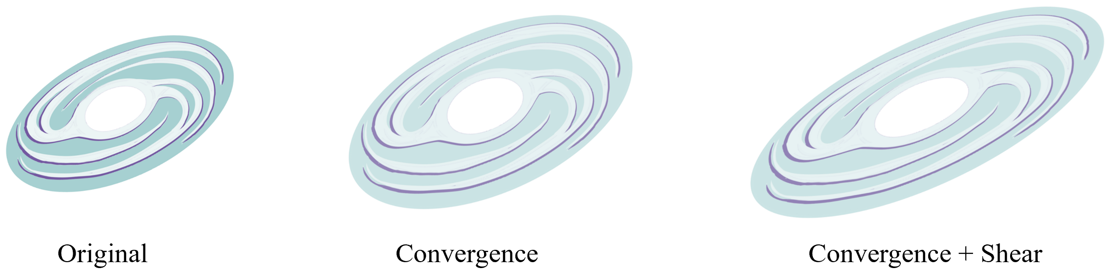
Figure 7: A cartoon demonstrating the difference between convergence and shear. Convergence isotropically changes the apparent size of a galaxy while conserving surface brightness, demonstrated here by a fainter color. Shear elongates the galaxy.

3.3 Shear: References

• “A method for weak lensing observations” Kaiser et al. (1995)
  Describes the motivation for measuring shear and how to model the shear response.

• “Weak gravitational lensing” Bartelmann & Schneider (2001)
  Comprehensive review of all aspects of weak lensing.

• “Cosmology with cosmic shear observations: a review” Kilbinger (2015)
  More recent review of all aspects of cosmic shear.

• “Weak gravitational lensing” Bartelmann & Maturi (2017)
  Basic introduction to concepts, assuming little prior knowledge.

• “Weak Lensing for Precision Cosmology” Mandelbaum (2018)
  Review of weak lensing in modern cosmology

4 IA Correlation Function Notation

The observed shape-density and shape-shape correlations are the result of several different combinations of effects. For example, these can include tidal alignments and “extrinsic” alignments, such as weak lensing. This section describes the notation most commonly used to denote these effects, while Section 5 describes methods to quantify their correlations.

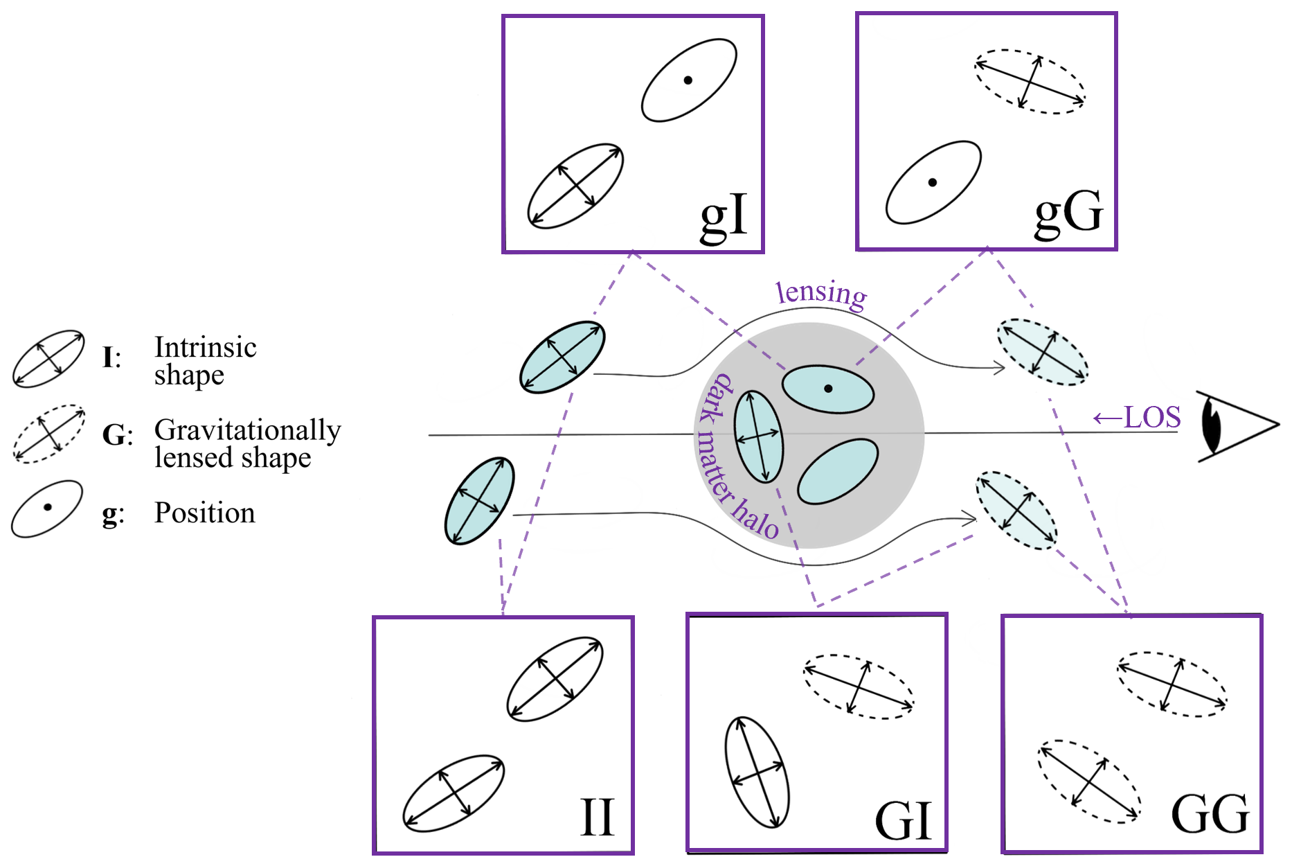
Figure 8: A schematic of correlations relevant to IA and weak lensing studies, shown along the LOS. Here, two background galaxies are lensed by a foreground dark matter halo. The observed shape $\epsilon$ of a galaxy is a combination of its intrinsic (I) and lensed (G) components. These are correlated with the underlying dark matter density, which can be traced by galaxy shapes and positions (g). Correlations are represented by combining these notations. For example, gI is the correlation between galaxy positions and intrinsic galaxy shapes, and GI is the correlation between the lensed component of galaxy shapes and intrinsic galaxy shapes. GI correlations are important because overdensities cause IA between galaxies at the same redshift while also lensing more distant galaxies. Separating galaxies into widely-spaced tomographic bins can distinguish between the GI and II terms (Section 4.2, Figure 9). For other helpful diagrams of IA correlations, see Figure 1.6 of Fortuna (2021) and Figure 6 of Troxel & Ishak (2015).
Note that this is a cartoon; galaxy shapes, orientations, and positions are only symbolic. These correlations are never measured for individual galaxies and are typically only statistically significant when measured for at least $10^{4}$ objects.

4.1 Correlations: Formalism

The main correlated components relevant to IA are the intrinsic shape of galaxies, the component of the shape which is gravitationally lensed, and the position of galaxies (Figure 8). For observed correlations that are measured as a function of sky separation, these are most commonly notated as

• I: intrinsic galaxy shape.

• G: lensed component of shape, also referred to as “extrinsic” shape.

• g: galaxy position (used as a tracer).

The observed shape-shape correlation $\langle\epsilon_{i}\epsilon_{j}\rangle$ between galaxies in two radial bins, $i$ and $j$, is the sum of every G and I combination:

$$\langle\epsilon_{i}\epsilon_{j}\rangle=\langle\text{G}_{i}\text{G}_{j}\rangle+\langle\text{G}_{i}\text{I}_{j}\rangle+\langle\text{I}_{i}\text{G}_{j}\rangle+\langle\text{I}_{i}\text{I}_{j}\rangle$$ (31)

These effects don’t necessarily sum mathematically (see the note above on shear addition). The notation $\langle X_{i}Y_{j}\rangle$ indicates the correlation of a quantity $X$ of a sample $i$ relative to quantity $Y$ of sample $j$ (Section 5.1). For example, $\langle\text{G}_{i}\text{I}_{j}\rangle$ is the correlation between lensed galaxy shapes of one sample relative to the intrinsic shapes of another sample. For binning along the LOS (see Section 4.2 on tomography), if $i$ is in a closer radial bin than $j$ then $\langle\text{G}_{i}\text{I}_{j}\rangle$ will be 0 since lensed shapes are created by a foreground mass. Therefore, either the second or the third term of Eq. (31) will be equal to zero. The first term of Eq. (31) is the shear correlation which is of interest for weak lensing studies but cannot be directly measured because the observed signal includes the IA term. The last term is the correlation between intrinsic ellipticities. Similarly, the observed galaxy shape-density correlation $\langle\epsilon_{i}n_{j}\rangle$ contains contributions from cross terms between lensed shape and density, and intrinsic shape and density,

$$\langle\epsilon_{i}n_{j}\rangle=\langle\text{G}_{i}n_{j}\rangle+\langle\text{I}_{i}n_{j}\rangle\,.$$ (32)

The observed galaxy number density is the sum of the intrinsic number density g and a lensing magnification component $m$ due to foreground overdensities (see the note above on convergence). This expression can then be written as

$$\langle\epsilon_{i}n_{j}\rangle=\langle\text{G}_{i}\text{g}_{j}\rangle+\langle\text{I}_{i}\text{g}_{j}\rangle\ +\langle\text{G}_{i}m_{j}\rangle\ +\langle\text{I}_{i}m_{j}\rangle\,,$$ (33)

where $\langle\text{G}_{i}\text{g}_{j}\rangle$ is usually called the galaxy-galaxy lensing signal. See Joachimi & Bridle (2010) for a cosmological analysis using a joint treatment of galaxy ellipticity, galaxy number density, and their cross-correlations.

4.2 Correlations: Additional Notations

• $+$: As defined in Section 2.1, the component of shape relative to the direction of the tidal field.

• $\times$: As defined in Section 2.1, the component of shape relative to $\frac{\pi}{4}$-off the direction of the tidal field.

• $T$ or $t$: the “tangential” component of shape, equivalent to $+$ (Hilbert et al., 2017).

• $\gamma_{\text{obs}}$: total observed shape, similar to $\epsilon$.

• $\gamma$: gravitational shear, or the correlation between lensed shapes. Equivalent to GG. Also sometimes used as the total observed shape.

• $\delta_{g}=\frac{g-\bar{g}}{\bar{g}}$: fractional overdensity, often used interchangeably with g.

• $\delta_{\text{m}}$: fractional overdensity of matter, as opposed to overdensity traced by galaxies. Sometimes notated as just $\delta$.

• $m$: sometimes used to refer to magnification from lensing, see Section 3.2.

• $\eta_{e}$: correlation between the 3D shape of a galaxy and position of another galaxy (Tenneti et al., 2015; Chisari et al., 2015). This is different from the lensing parameter in Section 3.

• $\eta_{s}$: correlation between the spin direction of a galaxy and position of another galaxy (Chisari et al., 2015).

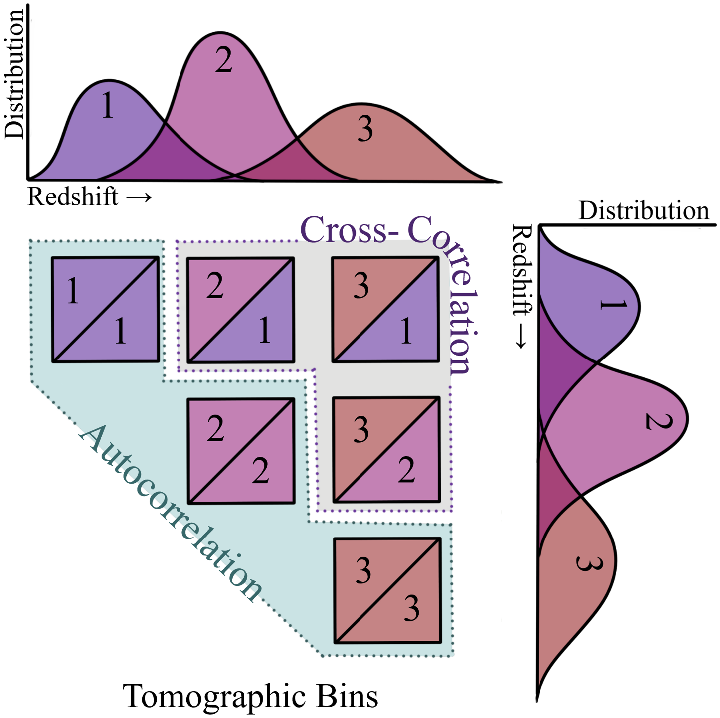
Figure 9: An illustrative example of binning used to measure cosmic shear. The initial redshift distribution is sliced into three tomographic bins (real surveys typically use more). The redshift distributions shown on the vertical and horizontal axes can be from the same or different samples. The boxes are number- and color-coordinated to show the six different combinations for correlations. If the correlations are done within the same bin, they are referred to as auto-correlations. Correlations between different bins are called cross-correlations.

Additional note: tomography

Tomography in the context of cosmological correlations refers to the technique where the redshift distribution of galaxies, $n(z)$, is sliced into redshift bins, also referred to as tomographic bins. This method allows extraction of additional information from correlations within the galaxy sample which would otherwise be projected out, for example the growth of structure as a function of time. Binning can be done so that bins are equally separated in redshift, so that there is an equal number of galaxies in each bin, or some combination of the two. If correlations are measured inside one bin, they are called “auto-correlations”. Correlations between galaxies in different tomographic bins are referred to as “cross-correlations”. Both spectroscopic and photometric surveys utilize the tomographic technique. In spectroscopic surveys, it is possible to avoid the overlapping of redshift bins. This is not possible in photometric surveys because the redshifts are not known precisely or accurately enough. For more information on the rationale for tomography, see Hu (1999).

4.3 Correlations: References

• “The correlation function of galaxy ellipticities produced by Gravitational Lensing” Miralda-Escude (1991)
  Historical documentation of ellipticity correlations.

• “Intrinsic alignments of galaxies in the Horizon-AGN cosmological hydrodynamical simulation” Chisari et al. (2015)
  Defines formalisms used in correlations of 3D shapes and spins.

• “Intrinsic alignments of disc and elliptical galaxies in the MassiveBlack-II and Illustris simulations” Tenneti et al. (2016)
  Defines additional formalisms used in 3D correlations.

5 IA Correlation Function Estimators

Correlations between the components described in Section 4 are quantified using the correlation function $\xi$. This is often measured as a function of separation of pairs along the LOS ($\Pi$) and in the transverse direction ($r_{p}$). Since we are dealing with pairs, these functions are called two-point correlation functions (2PCF). As opposed to the power spectra estimators described in the next sections, these correlation functions are less sensitive to survey geometry. In practice, most observations measure the projection of $\xi$ along the LOS $w_{p}$. While this contains less information than the full 3D correlations, it is more straightforward to observe and model, particularly when used in weak lensing analyses.

5.1 IA Correlation Function: Formalism

The IA correlation function is most commonly measured using a generalized form of the Landy-Szalay (LS) estimator, which was devised to estimate galaxy clustering (Landy & Szalay, 1993). This estimator accounts for systematics and has less variance than other estimators since it uses overdensity instead of density. To include information about alignment, the counts of galaxy pairs are weighted by the degree to which components are correlated (Mandelbaum et al., 2006).

The count of galaxy pairs between sample $A$ and $B$ is notated as $AB$. The count weighted by the correlation between shapes in $A$ and the positions of $B$ is $A_{+}B$:

$$A_{+}B=\sum_{i\in A,j\in B}\epsilon_{+}(j|i)\,,$$ (34)

The count weighted by the correlation between shapes in $A$ and shapes in $B$ is $A_{+}B_{+}$:

$$A_{+}B_{+}=\sum_{i\in A,j\in B}\epsilon_{+}(j|i)\epsilon_{+}(i|j)\,.$$ (35)

Here, $\epsilon_{+}(j|i)$ represents the $+$ component of the ellipticity of galaxy $j$ relative to the vector between it and the galaxy $i$ (Section 2). As described in Section 2.1, $0<\epsilon_{+}<1$ indicates radial alignment and $-1<\epsilon_{+}<0$ indicates tangential alignment.

Consider a galaxy shape catalogue, $S$, and a galaxy position catalog, $D$ ($D$ for density tracer s). These can be from the same sample. $S_{+}$ and $S_{\times}$ represent the relative $+$ and $\times$ component of shapes, as described in Eq.s 34, 35. $R_{D}$ and $R_{S}$ are randoms for the respective datasets: generated data designed to match the survey geometry but with no correlations. The correlation functions are

$$\xi_{gg}(r_{p},\Pi)=\frac{SD-R_{S}D-SR_{D}+R_{S}R_{D}}{R_{S}R_{D}}\,,$$ (36)

$$\xi_{g+}(r_{p},\Pi)=\frac{S_{+}D-S_{+}R_{D}}{R_{S}R_{D}}\,,$$ (37)

$$\xi_{++}(r_{p},\Pi)=\frac{S_{+}S_{+}}{R_{S}R_{S}}\quad\text{and}\quad\xi_{\times\times}(r_{p},\Pi)=\frac{S_{\times}S_{\times}}{R_{S}R_{S}}\,.$$ (38)

Note that $\langle S_{+}\rangle=\langle S_{\times}\rangle=0$, which allows us to disregard the contribution of $S_{+}R_{+}$ and $S_{\times}R_{\times}$ to first order due to systematic effects.

Projected Correlation Function
Most IA observations measure these correlation functions integrated along the LOS $\Pi$. The projected correlation function between two properties $a$ and $b$ is

$$w_{ab}(r_{p})=\int_{-\Pi_{\text{max}}}^{\Pi_{\text{max}}}\mathrm{d}\Pi\,\xi_{ab}(r_{p},\Pi)\,.$$ (39)

In practice, this requires a choice of how far along the LOS to integrate ($\Pi_{\text{max}}$) and in what size bins ($\mathrm{d}\Pi$). Typical values for these are comoving distances of $\Pi_{\text{max}}=100h^{-1}$Mpc, $\mathrm{d}\Pi=10h^{-1}$Mpc (Singh et al., 2015).

3D IA correlation function
The IA correlation function can be measured in 3D space, such as $\xi_{g+}(r_{p},\Pi)$ and $\xi_{++}(r_{p},\Pi)$, or the equivalent for the $\times$ component. It can also be quantified through the monopole and quadrupole components of IA correlation as a function of the redshift-space separation, $s$, $\xi_{g+}(s)$ or $\xi_{++}(s)$ (Singh & Mandelbaum, 2016; Okumura & Taruya, 2023). While more complicated to measure and model, these estimators can extract significantly more information from a survey (Singh et al., 2023).

Variable definitions

• $\xi$: usually used to denote a correlation function.

• $\xi_{gg}$: galaxy clustering, i.e., galaxy position-position correlation.

• $\xi_{g+}$: cross correlation of galaxy positions and intrinsic ellipticities.

• $\xi_{++},\xi_{\times\times}$: intrinsic shear shape-shape correlation.

• $D$: positions of sample used as a density tracer.

• $S$: positions of sample used for shape measurements.

• $R_{D}$: positions of random points made to match the spatial distribution of galaxy sample $D$ but with no spatial correlations.

• $R_{S}$: positions of random points corresponding to $S$.

• $S_{+}$: shapes of galaxies in shape sample.

• $w_{ab}$: projected correlation function.

• $\Pi$: distance along the LOS. $\Pi_{\text{max}}\sim 100h^{-1}$Mpc.

• $r_{p}$: distance transverse to the LOS.

5.2 IA Correlation Function: Additional Notations

• Alternative estimators similar to the LS estimators, are, for example (Joachimi et al., 2011)

  $$\xi_{g+}(r_{p},\Pi)=\frac{S_{+}D-S_{+}R_{D}}{D_{S}R_{D}}\,,$$ (40)

  The advantages of using the LS estimator are that it is less affected by survey geometry and has a higher signal-to-noise ratio (Singh et al., 2015).

• Another common way of denoting correlation functions is to write $\xi_{\gamma g}(r_{p},\Pi)=\langle\gamma(r_{p})g(r_{p}^{\prime})\rangle$.

• The projected correlation function is also notated as $w_{p}$.

• Sometimes the projected correlation function is integrated from $0-\Pi_{\text{max}}$ instead of $\pm\Pi_{\text{max}}$, in which case $\xi$ should be multiplied by 2.

• Correlation functions can also sometimes be expressed in terms of angles, such as $\xi(\bm{\vartheta})$ (or $\omega(\bm{\vartheta})$), in which case $\bm{\vartheta}$ is the 2D vector $\vec{\bm{\vartheta}}=(\vartheta_{1},\vartheta_{2})$, measured in the plane perpendicular to the LOS.

5.3 IA Correlation Function: References

• “Galaxy Alignments: Observations and Impact on Cosmology” Kirk et al. (2015)
  Contains a pedagogical, in-depth discussion of different IA correlation function estimators.

• “The correlation function of galaxy ellipticities produced by gravitational lensing” Miralda-Escude (1991)
  Original formalism for combining shape information in correlation functions.

• “The WiggleZ Dark Energy Survey: Direct constraints on blue galaxy intrinsic alignments at intermediate redshifts” Mandelbaum et al. (2011)
  Definitions of the generalized SZ IA estimators and helpful descriptions.

• “Intrinsic alignments of SDSS-III BOSS LOWZ sample galaxies” Singh et al. (2015)
  and “Intrinsic Alignments of BOSS LOWZ galaxies II: Impact of shape measurement methods” Singh & Mandelbaum (2016)
  Contain condensed definitions of IA correlation functions with most commonly used notation.

Additional note: estimators derived from shear correlation functions
Rather than using shear correlation function s directly, other estimator s derived from them may be preferred, for example to obtain higher signal-to-noise ratios or to control the physical scales used. In weak lensing studies, derived estimators are often chosen because they separate $E$-mode s from $B$-mode s. Lensing does not produce $B$-mode s so their detection in cosmic shear data could mean that the signal is affected by systematic effects such as IA.

The references below introduce three common derived estimators: complete orthogonal sets of E/B integrals (COSEBIs), aperture mass statistics, and band powers, and include their use for IA studies.

• “KiDS-1000 cosmology: Cosmic shear constraints and comparison between two point statistics” Asgari et al. (2021)
  Discusses pros and cons of estimators.

• “COSEBIs: Extracting the full E-/B-mode information from cosmic shear correlation functions” Schneider et al. (2010)
  Introduces COSEBIs as a method to separate E- and B-modes whilst retaining cosmological information.

• “Analysis of two-point statistics of cosmic shear” Schneider et al. (2002)
  Illustrates use of aperture mass statistics and band powers.

• “Sources of contamination to weak lensing three-point statistics: Constraints from N-body simulations” (Semboloni et al., 2008)
  Example of using aperture mass statistics to measure IA in simulations.

6 3D IA Power Spectrum

The power spectrum is perhaps the most basic statistic that can be used to describe density fields. By definition, the power spectrum is the mean square of the density fluctuation amplitudes. It is a function of wavenumber $k$ (Fourier space) or a multipole $\ell$ (spherical harmonics space) and is directly connected to the correlation function (Hikage et al., 2019).

The IA power spectrum described in this section quantifies the correlation between intrinsic galaxy shapes and the galaxy (or mass) density field in Fourier space. It is a 3D quantity which can be modeled directly or measured from simulations and is most often used to study IA directly. For a visualization of a typical IA power spectrum, see Figure 2 of Kurita et al. (2021).

6.1 3D IA Power Spectrum: Formalism

The Fourier transform of the intrinsic shear, $\gamma_{\text{I}}$, can be written as

$$\gamma_{\text{I}}(\bm{k}) =\gamma_{1}(\bm{k})+i\gamma_{2}(\bm{k})$$ (41)

$$\equiv\gamma(\bm{k})e^{-2i\phi_{\bm{k}}}\,,$$

where $\phi_{\bm{k}}$ is the angle measured from the first coordinate axis to $\bm{k}_{\perp}\equiv\sqrt{(k_{1}^{2}+k_{2}^{2})}$, the wave vector on the sky plane, so that $\phi_{\bm{k}}=\arctan(k_{1}/k_{2})$.

The galaxy-intrinsic power spectrum can be calculated from the correlation function of the galaxy density, g, and shear, $\gamma$,

$$P_{g\gamma}(\bm{k}) =\int\int\text{d}^{2}r_{p}\int\operatorname{d}\!{\Pi}\ e^{-i2\phi}e^{i\bm{k}\cdot\mathbf{r}}\xi_{g\gamma}(r_{p},\Pi)$$ (42)

$$=\int r_{p}\operatorname{d}\!{r}_{p}\int\operatorname{d}\!{\Pi}\ \xi_{g\gamma}(r_{p},\Pi)\int\operatorname{d}\!{\phi}\ e^{-i2\phi}e^{ikr\cos\phi}$$

$$=\int r_{p}\operatorname{d}\!{r}_{p}\int\operatorname{d}\!{\Pi}\ \xi_{g\gamma}(r_{p},\Pi)J_{2}(kr_{p})\,,$$

where $\vec{\bm{r}}=(r_{p},\Pi)$ and $\xi_{g\gamma}(r_{p},\Pi)=\langle g(r_{p},\Pi)\gamma(r_{p},\Pi)\rangle$ (Mandelbaum et al., 2011) and $J_{2}(kr_{p})$ is a Bessel function of the first kind.

We can also decompose the shear into its $E$- and $B$- modes, which are coordinate-independent quantities in Fourier space,

$$\gamma_{E}(\bm{k})+i\gamma_{B}(\bm{k})\equiv\gamma(\bm{k})e^{-2i\phi_{\bm{k}}}\,.$$ (43)

The $E$-mode $P_{gE}(\bm{k})$ and $B$-mode $P_{gB}(\bm{k})$ power spectra correspond to the real and imaginary part of $P_{g\gamma}$, respectively.

Similarly, other types of IA power spectra are

$$(2\pi)^{3}\delta_{D}(\bm{k}+\bm{k}^{\prime})P_{EE}(\bm{k})\equiv\langle\gamma_{E}(\bm{k})\gamma_{E}(\bm{k}^{\prime})\rangle\,,$$ (44)

$$(2\pi)^{3}\delta_{D}(\bm{k}+\bm{k}^{\prime})P_{\delta E}(\bm{k})\equiv\langle\gamma_{E}(\bm{k})\delta_{\text{m}}(\bm{k}^{\prime})\rangle\,,$$ (45)

where $\delta=\delta_{\text{m}}$ is the matter density field, and $\delta_{D}$ is the Dirac delta function. Equivalently, we have,

$$P_{EE}(\bm{k})=\int\text{d}^{2}r_{p}\operatorname{d}\!{\Pi}\ e^{-i\bm{k}\cdot\mathbf{r}}\xi_{EE}(r_{p},\Pi)\,,$$ (46)

$$P_{E\delta}(\bm{k})=\int\text{d}^{2}r_{p}\operatorname{d}\!{\Pi}\ e^{-i\bm{k}\cdot\mathbf{r}}\xi_{E\delta}(r_{p},\Pi)\,.$$ (47)

The $B$-mode power spectra, $\langle\gamma_{B}\gamma_{B}\rangle=0$ for IA caused by the scalar tidal field in the linear regime. $\langle g\gamma_{B}\rangle$ and $\langle\gamma_{E}\gamma_{B}\rangle$ should also vanish due to statistical parity invariance of the Universe. Note that, although $E$-mode and $B$-mode shear are defined in the 2D plane perpendicular to the LOS direction, the power spectra are functions of the 3D wave vector, $\bm{k}$. In other words, they are functions of $k=|\bm{k}|$ and the direction of $\bm{k}$.

Variable definitions

• $\bm{k}$: 3D wave vector.

• $\gamma_{E}(\bm{k})=\gamma_{1}(\bm{k})\cos{2\phi_{\bm{k}}}+\gamma_{2}(\bm{k})\sin{2\phi_{\bm{k}}}$, $E$-mode shear generated by the scalar gravitational potential.

• $\gamma_{B}(\bm{k})=-\gamma_{1}(\bm{k})\sin{2\phi_{\bm{k}}}+\gamma_{2}(\bm{k})\cos{2\phi_{\bm{k}}}$, $B$-mode shear cannot be generated by the scalar field in the linear regime, used as a check for systematic errors.

• $P_{EE}(\bm{k})$: auto power spectrum of the $E$-mode shear field, i.e., the intrinsic shape correlation signal.

• $P_{E\delta}(\bm{k})$: cross power spectrum between the $E$-mode shear and the mass density field, i.e., the GI signal.

Additional note: Alternative notation for 3D IA power spectra

Any of the above power spectra can also be expressed as

$$(2\pi)^{3}\delta_{D}(\bm{k}-\bm{k}^{\prime})P{(\bm{k})}=\langle\gamma(\bm{k})\gamma^{*}(\bm{k}^{\prime})\rangle\,,$$ (48)

where ^∗ is the complex conjugate, $P{(\bm{k})}$ is any one of the 3D IA power spectra and $\gamma$ denotes the intrinsic shear (or one of its components such as $\gamma_{E}$).

Additional note: multipole moments

Multipole moments of the IA power spectrum (Kurita et al., 2021) can be defined as

$$P_{XY}^{(\ell)}(k)=\frac{2\ell+1}{2}\int^{1}_{-1}\mathrm{d}\mu\mathcal{L}_{\ell}(\mu)P_{XY}(k,\mu),$$ (49)

where $P_{XY}(k,\mu)$ is one of the power spectra defined in Eqs. (42), (44) or (45), $\mu$ is the cosine of the angle between $\bm{k}$ and the LOS direction, $\mathcal{L}_{\ell}$ is the Legendre polynomial. $P^{(0)}$ is the monopole component, $P^{(2)}$ is the quadrupole component, and $P^{(4)}$ is the hexadecapole component. These can be used to quantify information about anisotropic effects.

Additional note: relation with correlation function

The relation between the correlation function and power spectrum can be written as

$$\langle[\gamma_{E}(\bm{k})+i\gamma_{B}(\bm{k})]g(\bm{k}^{\prime})\rangle =\langle\gamma(\bm{k})g(\bm{k}^{\prime})\rangle e^{-2i\phi_{\bm{k}}}$$

$$\equiv(2\pi)^{3}\delta_{D}(\bm{k}+\bm{k}^{\prime})P_{g\gamma}(\bm{k})\,,$$ (50)

where $\delta_{D}(\bm{k}+\bm{k}^{\prime})$ is the 3D Dirac delta function. Or, equivalently:

$$\xi_{g\gamma}(\mathbf{r})=\int\frac{\mathrm{d}\bm{k}}{(2\pi)^{3}}\,P_{g\gamma}(\bm{k})e^{2i(\phi_{\bm{k}}-\phi_{\mathbf{r}})}e^{i\bm{k}\cdot\mathbf{r}}.$$ (51)

For observations, this expression can also be written as

$$\xi_{AB}(r_{p},\Pi,z)=\int\frac{d^{2}k_{\perp}dk_{z}}{{(2\pi)^{3}}}P_{AB}(k,z)(1+\beta_{A}\mu^{2})(1+\beta_{B}\mu^{2})e^{i(r_{p}k_{\perp}+\Pi k_{z})}\,,$$ (52)

where $A,B\in\{g,+,\times\}$. $\beta$ models the effect of redshift-space distortions. $\beta_{+}=0$ and $\beta_{\times}=0$ to first order in the case of shear, and $\beta_{g}=f/b_{g}$ in the case of galaxies, where $f$ is the structure growth rate and $b_{g}$ the galaxy bias (Singh & Mandelbaum, 2016).

6.2 3D IA Power Spectrum: References

• “Power spectrum of halo intrinsic alignments in simulations” Kurita et al. (2021)
  Formalism and first measurement in N-body simulation.

• “Power spectrum of intrinsic alignments of galaxies in IllustrisTNG” Shi et al. (2021)
  IA power spectrum of galaxies in IllustrisTNG.

• “Analysis method for 3D power spectrum of projected tensor fields with fast estimator and window convolution modeling: An application to intrinsic alignments” Kurita & Takada (2022)
  Methodology for measuring IA power spectrum in observation.

• “Three-point intrinsic alignments of dark matter haloes in the IllustrisTNG simulation” Pyne et al. (2022)
  Extends formalism to three-point statistics.

7 2D IA Power Spectrum

The cosmic shear field is projected onto the plane of the sky and so the power spectrum used for weak lensing is also projected and therefore 2D. It can be defined in Fourier space ($P(k)$) or in spherical harmonic space (the angular power spectrum $C(\ell)$, or simply $C_{\ell}$). In this section we focus on the latter Note that terminology is often used quite loosely and both $P(k)$ and $C(\ell)$ may be referred to as the shear power spectrum.

In terms of the multipole moments of the 3D IA power spectrum, discussed in Section 6, the IA power spectrum relevant to cosmic shear analysis is the one evaluated at $\mu=0$, i.e., $P_{\delta E}(k,\mu=0)\equiv P_{\delta E}(k_{\perp})$, where $k_{\perp}=k(1-\mu^{2})^{1/2}$.

Power spectra can be expressed in terms of corresponding correlation function s. In the case of IA there is a family of correlation functions to choose from (see Kiessling et al. (2015) and Section 5). An example is the galaxy position-ellipticity correlation function $w_{g+}(r_{p})$:

$$w_{g+}(r_{p})=-b_{g}\int\operatorname{d}\!{z}\ W(z)\int_{0}^{\infty}\frac{\operatorname{d}\!{k}_{\perp}k_{\perp}}{2\pi}J_{2}(k_{\perp}r_{p})P_{\delta I}(k_{\perp},z)\,.$$ (53)

Here $P_{\delta I}(k_{\perp},z)$ corresponds to $P_{\delta E}(k_{\perp},z)$ in Section 6. The quantity $b_{g}$ is the galaxy-dark matter bias which is assumed here to be linear and scale-independent. These assumptions are justifiable for quasi-linear scales where perturbation theory applies, and assuming that on these scales structure formation is entirely determined by gravity (Desjacques et al., 2018). At smaller scales other considerations come into play and linear bias cannot safely be assumed.

Variable definitions

• $r_{p}$: transverse separation, as described in Section 2.

• $b_{g}$: galaxy-dark matter bias.

• $z$: redshift.

• $W(z)$: redshift weighted window function (Mandelbaum et al., 2011).

• $k_{\perp}$: wave vector perpendicular to the LOS.

• $J_{2}(k_{\perp}r_{p})$: a Bessel function of the first kind.

• $P_{\delta I}(k_{\perp},z)$: represents the 3D density-ellipticity power spectrum.

The 3D IA power spectrum can be projected along the LOS to construct the 2D projected angular IA power spectrum $C_{\epsilon\epsilon}^{ij}(\ell)$ as the sum of the gravitational lensing part GG, gravitational-intrinsic GI, and intrinsic-intrinsic contribution II:

$$C_{\epsilon\epsilon}^{ij}(\ell)=C_{\mathrm{GG}}^{ij}(\ell)+C^{ij}_{\mathrm{GI}}(\ell)+C_{\mathrm{II}}^{ij}(\ell)\,.$$ (54)

Each contribution in the above expression is described in spherical harmonic space where $\ell$ is the angular frequency. Figure 10 shows the $C_{\ell}s$ for each of these components.

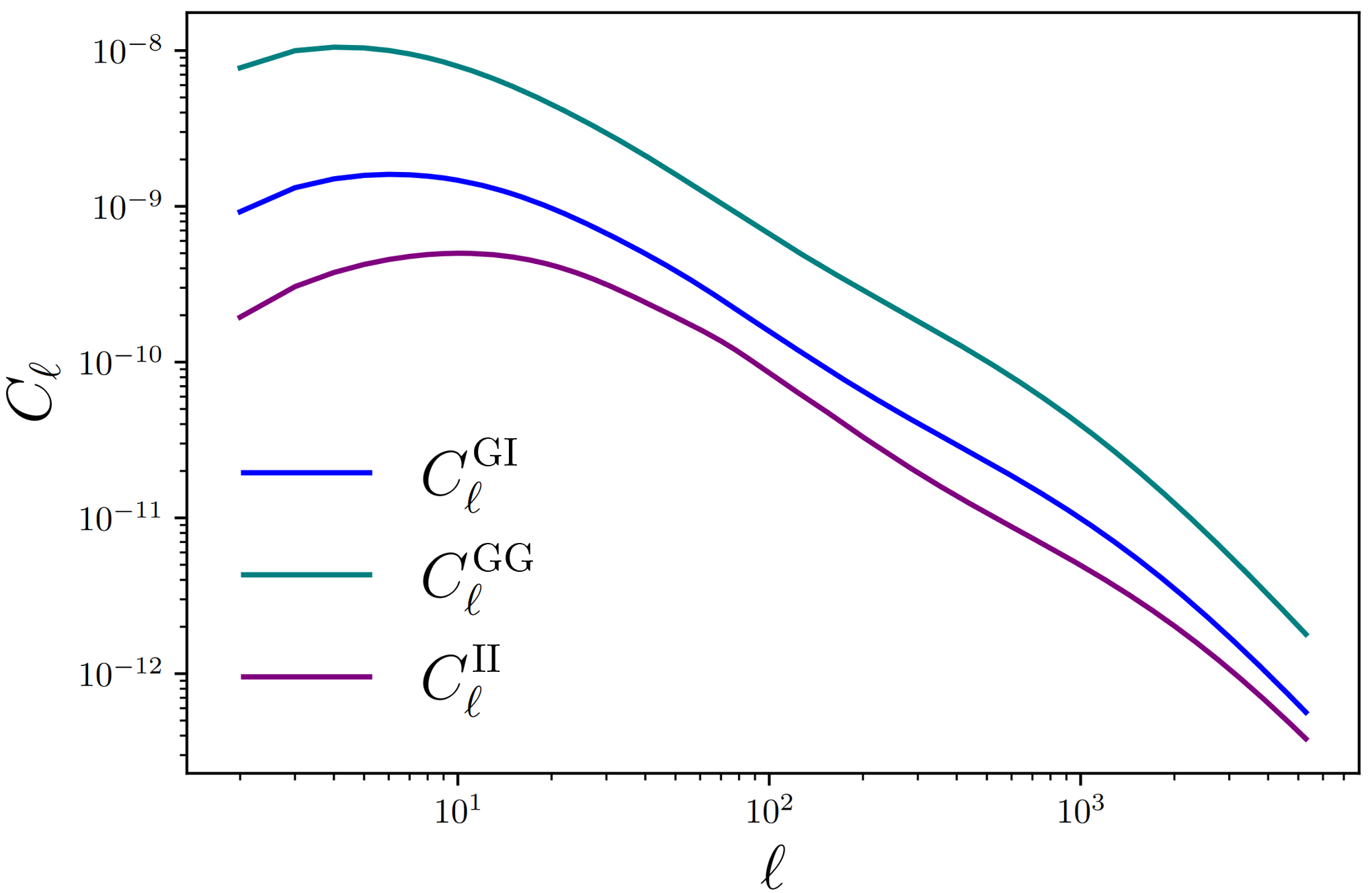
Figure 10: Angular power spectra for the different contributions given in Eq. (54). The $C_{\ell}^{\text{GI}}$ curve shows the absolute value for the component, as it is an anti-correlation. This plot was generated using the python package pyccl Chisari & Dvorkin (2013), assuming the nonlinear alignment model described in Section 8.3.

Indices $(i,j)$ represent two redshift bins in which the correlation is taking place (see Section 4.2). Terms in Eq. (54) can be represented as:

$$C_{\mathrm{GG}}^{ij}(\ell)=\int_{0}^{\chi_{\mathrm{H}}}\operatorname{d}\!{\chi}\frac{q^{i}(\chi)q^{j}(\chi)}{f^{2}_{K}(\chi)}P_{\delta\delta}\left(k=\frac{\ell}{f_{K}(\chi)},\chi\right)\,,$$ (55)

$$C_{\mathrm{GI}}^{ij}(\ell)=\int_{0}^{\chi_{\mathrm{H}}}\operatorname{d}\!{\chi}\frac{q^{i}(\chi)q^{j}(\chi)}{f^{2}_{K}(\chi)}P_{\delta\mathrm{I}}\left(k=\frac{\ell}{f_{K}(\chi)},\chi\right)\,,$$ (56)

$$C_{\mathrm{II}}^{ij}(\ell)=\int_{0}^{\chi_{\mathrm{H}}}\operatorname{d}\!{\chi}\frac{q^{i}(\chi)q^{j}(\chi)}{f^{2}_{K}(\chi)}P_{\mathrm{II}}\left(k=\frac{\ell}{f_{K}(\chi)},\chi\right)\,.$$ (57)

Section 8 discusses various methods used to model the power spectra $P_{\delta\mathrm{I}}$ and $P_{\mathrm{II}}$.

Variable definitions

• $\chi$ is the radial comoving distance.

• $\chi_{\mathrm{H}}$ is the comoving distance to the horizon.

• $f_{K}(\chi)$ is the radial function:

  $$f_{K}(\chi)=\begin{cases}\frac{1}{\sqrt{K}}\sin{(\sqrt{K}\chi)},&\text{if }\;\;K>0\;\;\text{(open universe)}\\ \chi,&\text{if }\;\;K=0\;\;\text{(flat universe)}\\ \frac{1}{\sqrt{-K}}\sinh{(\sqrt{-K}\chi)},&\text{if}\;\;K<0\;\;\text{(closed universe)}\par\end{cases}$$

  with $\frac{1}{\sqrt{|K|}}$ the curvature radius of the spatial part of spacetime.

• $q^{i}(\chi)$ and $q^{j}(\chi)$ are the lensing weighting functions in tomographic bins $i$ and $j$, respectively:

  $$q^{i}(\chi)=\frac{3H_{0}^{2}\Omega_{\text{m}}}{2c^{2}}\frac{f_{K}(\chi)}{a(\chi)}\int_{\chi}^{\chi_{\mathrm{H}}}\operatorname{d}\!{\chi}^{\prime}p^{i}(\chi^{\prime})\frac{f_{K}(\chi^{\prime}-\chi)}{f_{K}(\chi^{\prime})}\,,$$ (58)

  with $H_{0}$ the Hubble parameter, $\Omega_{\text{m}}$ the matter density fraction, $c$ the speed of light in a vacuum, and $a(\chi)$ the scale factor.

• $p^{i}(z)$ and $p^{j}(z)$ are galaxy redshift distributions in tomographic bins $i$ and $j$, respectively.

• $p^{i}(\chi)$ and $p^{j}(\chi)$ are the redshift distributions in tomographic bins $i$ and $j$, respectively, in radial comoving distance space: $p^{i}(\chi)=p^{i}(z)\frac{\operatorname{d}\!{z}}{\operatorname{d}\!{\chi}}$ and $p^{j}(\chi)=p^{j}(z)\frac{\operatorname{d}\!{z}}{\operatorname{d}\!{\chi}}$.

Limber Approximation

Power spectra on small scales (high multipoles $\ell$) are computationally expensive to calculate, especially if they involve rapidly oscillating functions. In practical applications, the Limber approximation is often used (Kitching et al., 2017; LoVerde & Afshordi, 2008). In this approximation the integrand varies more slowly but the result is still accurate at small scales.

One way to understand the approximation is to write the lensing angular power spectrum, $C_{\ell}^{\phi\phi}$, as (Lemos et al., 2017)

$$C_{\ell}^{\phi\phi}(r,s)=\frac{8}{\pi}\left(\frac{3\Omega_{\text{m}}^{2}H_{0}^{2}}{2c^{2}}\right)^{2}\int\frac{\operatorname{d}\!{k}}{k^{2}}\ I^{r}_{\ell}(k)I^{s}_{\ell}(k)\,,$$ (59)

where

$$I^{r}_{\ell}(k)=\int\frac{\mathrm{d}\chi}{\chi}\ [1+z(\chi)]q^{r}(\chi)j_{\ell}(k\chi)[P_{\delta}(k;\chi)]^{1/2}\,.$$ (60)

The Limber approximation replaces the spherical Bessel function $j_{\ell}(k\chi)$ with a delta function:

$$j_{\ell}(k\chi)\rightarrow\sqrt{\frac{\pi}{2\nu}}\delta_{D}(\nu-k_{\chi})\,,$$ (61)

with $\nu=\ell+\frac{1}{2}=k\chi$. Then the shear power spectrum takes the form:

$$C_{\ell}^{\epsilon\epsilon}(r,s)=\frac{(\ell+2)!}{\nu^{4}(\ell-2)!}\left(\frac{3\Omega_{\text{m}}^{2}H_{0}^{2}}{2c^{2}}\right)^{2}\int\operatorname{d}\!{\chi}\ [1+z(\chi)]^{2}q^{r}(\chi)q^{s}(\chi)P_{\delta}\left(\frac{\nu}{\chi};\chi\right)\,.$$ (62)

The Limber approximation assumes that the variation of the kernels of the projected fluctuations are limited to scales larger than the average clustering length, which makes it invalid across all scales. This limitation, combined with the need to reduce systematic errors for future cosmological surveys, require non-Limber methods. There have been recent efforts to move away from the Limber approximation in numerical analysis, such as in Leonard et al. (2023) which presents several alternatives to implement this calculation in a fast and reliable framework.

7.1 2D IA Power Spectra: Additional Notations

• $r$ and $s$: indices that denote two tomographic bins are usually $i$ and $j$. Some authors use $r$ and $s$ instead (for example Lemos et al. (2017))

• $W$: represents a window function. It is often called a filter function or a survey window. It can be defined in terms of many survey parameters such as redshift $z$, position on the sky $\theta$, etc.

• $n^{r}(\chi)$ and $n^{s}(\chi)$: often used in place of $p^{i}(\chi)$ and $p^{j}(\chi)$ to denote the redshift distributions in respective tomographic bins $i$ and $j$.

7.2 2D IA Power Spectra: References

• “Weak lensing power spectra for precision cosmology: Multiple-deflection, reduced shear and lensing bias corrections” Krause & Hirata (2010)
  Detailed derivation for the corrected weak lensing power spectra.

• “Cosmology from cosmic shear power spectra with Subaru Hyper Suprime-Cam first-year data” Hikage et al. (2019)
  Example of accounting for IA in power spectrum analysis of data from the Hyper Supreme-Cam (HSC).

• “KiDS-1000 cosmology: Cosmic shear constraints and comparison between two point statistics” Asgari et al. (2021)
  Short breakdown of the power spectra for KiDS survey. Has a good list of references.

Additional note: beyond the power spectrum
Power spectra are powerful probes of IA. However, lower-order statistics such as the power spectrum or 2PCF compress information in non-Gaussian and anisotropic fields, like the dark matter field in the weakly and strongly nonlinear regime. Ideally we want to ensure that high-order statistics (e.g., 3-point correlations (Schmitz et al., 2018) or entire fields) are taken into account in IA inferences and that uncertainties are accounted for self-consistently via forward modeling in weak lensing (see Porqueres et al. (2023) and references therein). A 3D inference of IA has been performed on existing galaxy datasets (Tsaprazi et al., 2022). With the advent of next-generation data these methods must be advanced to smaller scales in order to increase the signal-to-noise ratio of the detections.

8 Modeling

Many IA models have developed over the past couple decades and even the earlier ones are still useful. Advancements reflect the increasing understanding and importance of IA and the need to extend theory to smaller scales and a wider range of alignment mechanisms. Models are often created for specific scales and galaxy types, the main two being spiral and elliptical. As noted in Section 1, how these morphologies relate to ELG/LRG s is a source of discussion and the distinction between “red” and “blue” galaxy samples is survey and simulation-dependent.

Here we summarize the most commonly used IA models and point towards useful references for more information. In Sections 8.1-8.4 we discuss models which estimate the amplitude of the IA effect, starting with an explanation of the amplitude itself. Section 8.5 and Section 8.6 discuss two other modeling approaches: effective field theory and halo models. Section 8.7 and Table 1 summarize the observational status of the models. Finally, Section 8.8 briefly introduces self-calibration, a model-agnostic technique.

8.1 Alignment Amplitude

Alignment amplitude is an empirical constant which relates a measurement of the underlying density to the amplitude, or strength, of the IA signal. It is most commonly used as a parameter in models of the IA projected correlation function and the IA power spectrum. Some models include more than one amplitude parameter but where there is only a single parameter, it is often (but not always) denoted by $A_{\text{IA}}$. When cosmological parameters are estimated from weak lensing, $A_{\text{IA}}$ is often treated as a “nuisance” parameter to be marginalized over.

The amplitude is expected to evolve with redshift and also to depend on galaxy/halo mass. The redshift dependence is thought to arise because galaxies traverse regions of differing tidal shear due to their peculiar velocities (advection) (Schmitz et al., 2018) or because halo mass accretion is stronger at higher redshifts (Asgari et al., 2023). IA is generally expected to vary with luminosity because more luminous galaxies are typically younger and have less time to misalign (Blazek et al., 2011). In observational studies, luminosity is often used as a proxy for mass so that we have $A_{\text{IA}}(z,L)$.

All these dependencies are difficult to quantify in practice. Because of this, the redshift scaling is often separated into “low redshift” and “high redshift” contributions. Alternatively, the alignment amplitude is simply set to be constant across the redshift range. Observations have found $A_{\text{IA}}$ to be consistent with zero for blue galaxies (Johnston et al., 2019), suggesting lack of tidal alignment, but robust detections have been made for red galaxies e.g. Fortuna et al. (2021b). For this reason, the amplitude may be corrected for the fraction of red galaxies, or the two sub-samples analyzed separately.

In the sections below, we give a brief overview of the current models: Linear Alignment model (LA), Nonlinear Alignment model (NLA), Tidal Alignment and Tidal Torquing model (TATT), the Effective Field Theory (EFT), and the halo model.

8.1.1 IA Amplitude: Additional Notation

Although $A_{\text{IA}}$ is a common notation, the amplitude is sometimes denoted as $A$ or $A{\text{I}}$. However, one must be careful as they often represent different quantities depending on the model. Additionally, superscripts may be used to indicate the amplitude of subsamples e.g., $A_{\text{IA}}^{\text{R}}$, $A_{\text{IA}}^{\text{B}}$ for red and blue samples.

For models with more than one IA amplitude the notation $A_{1}$, $A_{2},\ldots$ is often used. In this case $A_{1}$ may also be used for the single-amplitude model.

8.1.2 IA Amplitude: References

• “Redshift and luminosity evolution of the intrinsic alignments of galaxies in Horizon-AGN” Chisari et al. (2016)
  A detailed work on the IA amplitude dependency on redshift and luminosity.

• “KiDS+GAMA: Intrinsic alignment model constraints for current and future weak lensing cosmology” Johnston et al. (2019)
  Dependency of IA amplitude on color in observations.

• “KiDS-1000: Constraints on the intrinsic alignment of luminous red galaxies” (Fortuna et al., 2021b)
  Luminosity and redshift dependence of IA for LRG s.

• “Advances in Constraining Intrinsic Alignment Models with Hydrodynamic Simulations” (Samuroff et al., 2021)
  Comprehensive analysis comparing multiple simulations and dependence of IA on galaxy properties.

8.2 Linear Alignment model (LA)

This approach assumes that the ellipticity of a galaxy (and hence $A_{\text{IA}}$) is linearly related to the gravitational potential at the time the galaxy formed. Before we start, it is useful to define two redshifts relevant for the LA and other models:

• $z_{\mathrm{IA}}$: the redshift at which the alignment is set.

• $z_{\mathrm{obs}}$: the redshift at which the IA is observed.

Since the details of galaxy formation and evolution are not well understood, two scenarios are proposed for the redshift $z_{\text{IA}}$ at which the alignment is produced.

• Instantaneous Alignment: In this case the alignment redshift is assumed to be the same as the observed redshift, $z_{\mathrm{IA}}=z_{\mathrm{obs}}$, and the IA amplitude is a simple linear function of redshift.

  $$A_{\mathrm{IA}}(z)=-C_{1}(z)\rho_{\text{m},0}(1+z)\,,$$ (63)

  where $C_{1}(z)$ is a contribution due to the response to the tidal field and $\rho_{\text{m},0}$ is the matter density at $z=0$ (today).

• Early Alignment: In the early alignment scenario, the redshift at which the IA signal is observed is later than the redshift at which the alignment was set, $z_{\mathrm{obs}}<z_{\mathrm{IA}}$. If it is assumed that the halo first forms during the matter domination era (primordial alignment) then $A_{\mathrm{IA}}$ does not depend on $z_{\mathrm{IA}}$ and evolves as

  $$A_{\mathrm{IA}}(z)=-\frac{C_{1}(z)\rho_{\text{m},0}(1+z)}{\bar{D}(z)}\,,$$ (64)

  where $\bar{D}(z)$ has been set to unity at matter domination: $\bar{D}(z)=(1+z)D(z)$, and $D(z)$ is the growth factor. It is often assumed that alignment happens later than this because it is affected by more recent mergers and accretion. Then the amplitude is given by:

  $$A_{\mathrm{IA}}(z)=-C_{1}(z)\rho_{\text{m},0}(1+z_{\mathrm{IA}})\frac{D(z_{\mathrm{IA}})}{D(z)}\,.$$ (65)

8.2.1 LA model: References

• “Intrinsic and extrinsic galaxy alignment” Catelan et al. (2001)
  Introduction of LA model.

• “Intrinsic alignment-lensing interference as a contaminant of cosmic shear” Hirata & Seljak (2004)
  Development of LA model.

• “Tidal alignment of galaxies” Blazek et al. (2015)
  Section 3.2 discusses alignment epochs.

8.3 Nonlinear Alignment model (NLA)

This is an empirical model which replaces the linear power spectrum used in the LA model with the full nonlinear matter power spectrum, $P_{\text{NL}}(k,z)$, while preserving the assumption that density perturbations are described by the Poisson equation. Physically, the latter assumption fails in the nonlinear regime of structure formation due to gravitational evolution. However, this model has been widely adopted due to its ability to accurately reproduce ellipticity correlations for red elliptical galaxies down to $\sim 6$ $h^{-1}$Mpc. The NLA model is often enhanced to include other sample dependencies, for example on redshift or galaxy luminosity, usually captured by additional power laws.

To incorporate a luminosity $L$ dependence, the IA amplitude $A_{\text{IA}}$ is expressed as a power law of the general form:

$$A_{\text{IA}}\mapsto A\left(\frac{L}{L_{0}}\right)^{\alpha_{L}}\,,$$ (66)

where $A$ is a prefactor, $L_{0}$ is a pivot luminosity and $\alpha_{L}$ is a luminosity scaling. Furthermore, the IA amplitude form can be extended to account for the redshift evolution as

$$A_{\text{IA}}(L,z)=A\left(\frac{L}{L_{0}}\right)^{\alpha_{L}}(1+z)^{\alpha_{z}}\,,$$ (67)

with $\alpha_{z}$ a redshift scaling parameter. This parameter is often denoted $\eta$ or, if the redshift contribution is separated into low- and high-redshift parts, $\eta_{\mathrm{low-z}}$ and $\eta_{\mathrm{high-z}}$. Not to be confused with the definition in Section 2.3 or in Section 4. For more details, consult Chisari et al. (2016).

Practical uses
Another parametrization of the redshift and luminosity dependent IA amplitude frequently used in analyses is:

$$A_{\mathrm{IA}}(L,z)=A_{0}\frac{C_{1}\rho_{\text{m},0}}{D(z)}\left(\frac{L}{L_{0}}\right)^{\alpha_{L}}\left(\frac{1+z}{1+z_{0}}\right)^{\alpha_{z}}\,,$$ (68)

where $A_{0}$ is a prefactor and $z_{0}$ is a pivot redshift. $C_{1}$, $\rho_{\text{m},0}$ and $D(z)$ are described in Section 8.2. Since the signal is not observed in blue galaxies, the amplitude is corrected for the fraction of red galaxies and the redshift scaling is often separated into “low redshift” and “high redshift” contribution. The details can be found in Krause et al. (2016).

8.3.1 NLA model: References

• “Dark energy constraints from cosmic shear power spectra: Impact of intrinsic alignments on photometric redshift requirements” Bridle & King (2007)
  First use of NLA model. The authors argue that this model might not be “closer to the truth”, but that it matches the data slightly better than the LA model.

• “Constraints on intrinsic alignment contamination of weak lensing surveys using the MegaZ-LRG sample” Joachimi et al. (2011)
  Frequently cited paper with values for constants in LA/NLA model.

• “Intrinsic alignments of SDSS-III BOSS LOWZ sample galaxies” Singh et al. (2015)
  Tests NLA model against observations.

• “The impact of intrinsic alignment on current and future cosmic shear surveys” Krause et al. (2016)
  Detailed description of the luminosity and redshift dependent IA amplitude.

8.4 Tidal Alignment and Tidal Torquing model (TATT)

The above models are strictly thought to apply only to elliptical galaxies. TATT was introduced to account for the alignment of spiral galaxies whose configuration depends on angular momentum rather than being pressure-supported. The basic idea is to express a galaxy’s intrinsic shape $\gamma^{\mathrm{I}}_{ij}$ as an expansion of the trace-free tidal field tensor $s_{ij}$ to second order in the linear density field:

$$\gamma^{\mathrm{I}}_{ij}=C_{1}s_{ij}+C_{1\delta}(\delta\times s_{ij})+C_{2}\bigg{[}\sum_{k=0}^{2}s_{ik}s_{kj}-\frac{1}{3}\delta_{ij}s^{2}\bigg{]}\,,$$ (69)

where $\delta$ and $s$ respectively describe the density and tidal fields. The first term corresponds to tidal alignment as in the LA/NLA models. The second is “density weighting” and arises because alignment can only be measured where there is a galaxy. The third term is tidal torquing. The tidal alignment is described by $C_{1}$,

$$C_{1}(z)=-A_{1}(z)\frac{\bar{C}_{1}\rho_{\text{m}}}{D(z)}\,,$$ (70)

with a similar formula for $C_{1\delta}$, which can be parameterized as $C_{1\delta}=b_{1}C_{1}$, where $b_{1}$ is called the linear bias. $A_{1}$ is equivalent to $A_{\mathrm{IA}}$ in the LA/NLA models. For the case of instantaneous alignment ($z_{\text{IA}}=z_{\text{obs}}$):

$$A_{1}(z)=-C_{1}(z)\rho_{\text{m},0}(1+z);$$ (71)

for earlier epochs of alignment:

$$A_{1}(z)=-C_{1}(z)\rho_{\text{m},0}(1+z_{\text{IA}})\frac{D(z_{\text{IA}})}{D(z)}\,;$$ (72)

and for primordial alignment during matter domination:

$$A_{1}(z)=-\frac{C_{1}(z)\rho_{\text{m},0}(1+z)}{\bar{D}(z)}\,,$$ (73)

with ${\bar{D}(z)}=D(z)(1+z)$, and $\bar{D}(z)=1$ during matter domination. The tidal torquing parameter, $C_{2}$, is given by

$$C_{2}(z)=A_{2}(z)\frac{5\bar{C}_{1}\rho_{\text{m}}}{D^{2}(z)}\,,$$ (74)

where $A_{2}$ is a second alignment amplitude. The factor 5 is an approximation related to the different IA power spectrum in the pure tidal alignment and tidal torquing cases.

8.4.1 TATT model: References

• “Beyond linear galaxy alignments” Blazek et al. (2019)
  Introduction of TATT model and full equations for IA power spectra.

• “Advances in constraining intrinsic alignment models with hydrodynamic simulations” Samuroff et al. (2021)
  2PCF measurements from simulations comparing NLA and TATT models (and comparing simulations). Contains helpful discussion of the models..

8.5 Effective Field Theory (EFT) model

EFT extends the modeling of IA to smaller scales in a more theoretically rigorous way than the NLA model. On large scales, the matter density distribution is treated as an effective fluid, while the small-scale physics are decoupled and packed into a set of free parameters with values that can be constrained through either simulations or observations. Since this approach includes higher spatial derivatives of the density and tidal field s, the modeling of IA is extended from linear scales to the quasi-linear regime.

This approach involves first capturing the physical interactions that give rise to intrinsic galaxy shape correlations within the galaxies’ rest frame. These correlations are then expressed in terms of local gravitational observables. This accounts for the statistical properties of galaxy shapes resulting from gravitational effects and allows for a systematic approach to modeling the corresponding IA. Next, the obtained statistical information is projected onto the sky, effectively mapping the correlations onto the observed galaxy shapes (Vlah et al., 2020). Presently this is the only IA model capable of characterizing the auto-spectrum of IA $B$-modes with high accuracy (Bakx et al., 2023).

8.5.1 EFT: References

• “An EFT description of galaxy intrinsic alignments” Vlah et al. (2020)
  EFT description of 3D IA.

• “Galaxy shape statistics in the effective field theory” Vlah et al. (2021)
  Projection onto the observed sky.

• “Effective field theory of intrinsic alignments at one loop order: a comparison to dark matter simulations” Bakx et al. (2023)
  Comparison of EFT of IA to simulations.

8.6 Halo model

The halo model is an alternative approach which does not directly model the IA amplitude. Instead, it builds on the halo model of galaxy clustering in which the power spectrum is modeled as the sum of a one-halo term corresponding to the (small-scale) correlation of galaxies within a single dark matter halo, and a two-halo term corresponding to the (large-scale) correlation of galaxies in different halos. Applied to IA, this allows for different modeling of the alignment of satellite and central galaxies. In particular it can be assumed that centrals have the same ellipticity and orientation as their parent halos and that this can be described by the linear alignment model. The two-halo term allows for different amplitudes for the alignment contribution of red and blue populations:

$$P^{\mathrm{2h}}_{\mathrm{GI}}(k)=f^{\mathrm{red}}_{\mathrm{c}}P^{\mathrm{red}}_{\mathrm{GI}}(k)+f^{\mathrm{blue}}_{\mathrm{c}}P^{\mathrm{blue}}_{\mathrm{GI}}(k)\,,$$ (75)

where the fraction of red and blue centrals, $f^{\mathrm{red}}_{\mathrm{c}}$ and $f^{\mathrm{blue}}_{\mathrm{c}}$, can be determined using a model of the halo occupation distribution. Under the assumption of a spherical halo, the inter-halo alignment between centrals and satellites is zero on average, and thus the one-halo term describes the alignment of satellites with each other and the local matter field:

$$P^{\mathrm{1h}}_{\mathrm{GI}}(k)=\int\operatorname{d}\!{M}n(M)\frac{M}{\bar{\rho}_{\text{m}}}f_{\mathrm{s}}\frac{\langle N_{\mathrm{s}}|M\rangle}{\bar{n}_{\mathrm{s}}}|\hat{\gamma}^{\mathrm{I}}(\boldsymbol{k}|M)|\hat{U}(M,k)\,,$$ (76)

where $n(M)$ is the halo mass function, $f_{\mathrm{s}}$ is the fraction of satellite galaxies, which can be written as a function of redshift, $\langle N_{\mathrm{s}}|M\rangle$ is the halo occupation distribution of satellites, $\hat{U}(M,k)$ is the normalized matter density profile, and $\hat{\gamma}^{\mathrm{I}}$ is the density-weighted average of the satellite intrinsic ellipticity. An additional dependence on radius can be included, and equivalent intrinsic-intrinsic power spectrum terms can be similarly derived.

The halo model has been shown to fit observations in the range $0.3-1.5$ $h^{-1}$Mpc (Singh et al., 2015), and on larger scales can be complemented by the LA or the NLA models. Although its formalism relies on physical assumptions, such as the symmetry of the halos or the alignment of satellites inside a halo, and it suffers from the lack of constraints for fainter galaxies, this model performs well in the context of weak lensing correction for current surveys.

Variable definitions

• $P^{\mathrm{2h}}_{\mathrm{GI}}(k)$: 2-halo term of the gravitational-intrinsic power spectrum.

• $f^{\mathrm{red}}_{\mathrm{c}},f^{\mathrm{blue}}_{\mathrm{c}}$: fractions of red and blue central galaxies.

• $P^{\mathrm{1h}}_{\mathrm{GI}}(k)$: 1-halo term of the gravitational-intrinsic power spectrum.

• $n(M)$: halo mass function.

• $f_{\mathrm{s}}$: fraction of satellite galaxies.

• $\langle N_{\mathrm{s}}|M\rangle$: halo occupation distribution of satellites.

• ${\bar{n}_{\mathrm{s}}}$: mean number density of galaxies.

• $|\hat{\gamma}^{\mathrm{I}}(\boldsymbol{k}|M)|$: density-weighted average satellite ellipticity.

• $\hat{U}(M,k)$: normalized matter density profile.

8.6.1 Halo model: References

• “Halo models of large scale structure” Cooray & Sheth (2002)
  Original halo model of galaxy clustering.

• “A halo model for intrinsic alignments of galaxy ellipticities” Schneider & Bridle (2010)
  First IA halo model.

• “The halo model as a versatile tool to predict intrinsic alignments” Fortuna et al. (2021a)
  Development of halo model for IA.

• “The halo model for cosmology: A pedagogical review” Asgari et al. (2023)
  Introduction to the halo model with some discussion of IA.

Table 1: Current consensus on the scale range of IA model validity and corresponding galaxy populations used to derive it.

Model	Scales [$h^{-1}$Mpc]	Galaxy type	Study
LA	$>$ 10	clusters	Chisari et al. (2014)
NLA	$>$ 6	LRG	Singh et al. (2015)
TATT	$>$ 2	LRG, ELG	Samuroff et al. (2022)
EFT	$>$ 0.3	LRG, ELG	Bakx et al. (2023)
Halo	0.3-1.5	LRG	Singh et al. (2015)

8.7 Modeling: Observational status

The assumption of the linearity of tidal shear breaks down on small scales. Therefore, alignment models that are more informed about nonlinear structure growth are required for accurate modeling of galaxy shapes. In Table 1, we report estimates of the scales at which the models discussed above are considered to accurately model ellipticity correlations. Chisari et al. (2014) reported that the linear alignment model behaves well only down to $10$ $h^{-1}$Mpc, whereas Singh et al. (2015) found that the nonlinear alignment model accurately models the ellipticities of luminous red galaxies down to $6$ $h^{-1}$Mpc. However, both these models seem to underestimate $A_{\text{IA}}$ on smaller scales. An accurate extension down to $2$ $h^{-1}$Mpc (Samuroff et al., 2022) is the TATT model. Finally, the halo model has been successfully used in the range $0.3-1.5$ $h^{-1}$Mpc (Singh et al., 2015), yet it lacks the ability to capture correlations in the mildly nonlinear regime.

8.8 Self-calibration

When weak lensing data is used to constrain cosmological parameters, an alternative to directly modeling IA and marginalizing over parameters is to follow a model-agnostic approach through self-calibration. This technique exploits cross-correlations with other survey observables and does not need any data external to the survey (for example to set priors on the IA parameters). The articles below are selected examples of self-calibration, ranging from its initial proposal to its application to recent survey data.

8.8.1 Self-calibration: References

• “Self-calibration of gravitational shear-galaxy intrinsic ellipticity correlation in weak lensing surveys” Zhang (2010)
  First paper on IA self-calibration.

• “Self-calibration for three-point intrinsic alignment autocorrelations in weak lensing surveys” Troxel & Ishak (2012)
  Useful overview and extends the concept to three-point statistics.

• “Self-calibration method for II and GI types of intrinsic alignments of galaxies” Yao et al. (2019)
  Review of methodology and forecast for LSST.

• “KiDS-1000: Cross-correlation with Planck cosmic microwave background lensing and intrinsic alignment removal with self-calibration” Yao et al. (2023)
  Comparison of self-calibration with other methods and application to KiDS data.

9 IA Applications

Although galaxy IA has been intensively studied as one of the most important systematic effects for weak lensing cosmology, it can cause other biases and has the potential to be a novel probe in cosmology. Here we list a selection of papers which describe some of these applications. As a direct result of galaxy formation mechanics, in principle IA can also be used to explore the relationship between the formation of galaxies and their dark matter environment. However, currently higher precision measurements and more detailed modeling are necessary before IA is useful for constraining galaxy formation, particularly on small scales.

9.1 Redshift-space distortion bias

When IA is combined with a bias in galaxy orientations due to a survey’s target selection, the survey can measure an enhanced clustering along the LOS. This anisotropic clustering effect mimics redshift space distortions (RSD), which are used to measure the growth of large-scale structure.

• “Tidal alignments as a contaminant of redshift space” Hirata (2009)
  First work that discussed orientation-dependent selection effects and IA on RSD measurements.

• “Detection of anisotropic galaxy assembly bias in BOSS DR12” Obuljen et al. (2020)
  Finds a correlation between galaxy orientation and anisotropic clustering in BOSS.

• “Impact of intrinsic alignments on clustering constraints of the growth rate” Zwetsloot & Chisari (2022)
  Contains a helpful theory discussion on this effect.

• “Intrinsic alignment as an RSD contaminant in the DESI survey” Lamman et al. (2023)
  Forecasts a significant impact on DESI’s RSD measurements from IA.

9.2 Cosmological applications

IA can be used to explore cosmological parameters through the impact that features such as RSD, Baryon Acoustic Oscillations (BAO) and Primordial Non-Gaussianity (PNG) have on the IA signal. Below is an incomplete list of papers discussing the use of IA to probe cosmology:

• “Imprint of inflation on galaxy shape correlations” Schmidt et al. (2015)
  The original paper on exploring PNG through IA.

• “Cosmological information in the intrinsic alignments of luminous red galaxies” Chisari & Dvorkin (2013)
  Forecasts for the ability of ongoing spectroscopic surveys to constrain local PNG and BAO in the cross-correlation function of IAs and the galaxy density field.

• “Intrinsic alignment statistics of density and velocity fields at large scales: Formulation, modeling, and baryon acoustic oscillation features” Okumura et al. (2019)
  The first detection of the BAO feature on IA, in N-body simulations.

• “The impact of self-interacting dark matter on the intrinsic alignments of galaxies” Harvey et al. (2021)
  Finds that self-interacting dark matter could suppress IA in a way distinct from potential baryonic effects.

• “The alignment of galaxies at the Baryon Acoustic Oscillation scale” van Dompseler et al. (2023)
  Gives a theoretical explanation of the characteristics of the BAO feature on IA.

• “Tightening geometric and dynamical constraints on dark energy and gravity: galaxy clustering, intrinsic alignment and kinetic Sunyaev-Zel’dovich effect” Okumura & Taruya (2022)
  Demonstration of the extra constraining power obtained by adding IA and kinetic Sunyaev-Zel’dovich to conventional clustering measurement, using Fisher matrix.

• “Constraints on anisotropic primordial non-Gaussianity from intrinsic alignments of SDSS-III BOSS galaxies” Kurita & Takada (2023)
  First constraints on anisotropic PNG using IA.

• “Imprint of anisotropic primordial non-Gaussianity on halo intrinsic alignments in simulations” Akitsu et al. (2021)
  Uses N-body simulations to show that IA can probe anisotropic PNG, while clustering cannot.

Author Contributions

The author order is lead, followed by the coauthors in reverse alphabetical order. All coauthors contributed equally.
C.L.: claire.lamman@cfa.harvard.edu
E.T.: eleni.tsaprazi@fysik.su.se
J.S.: jingjing.shi@ipmu.jp
N.S.: nikolina.sarcevic@gmail.com
S.P.: s.pyne@ucl.ac.uk
E.L.: elegnani@ifae.es
T.F.: tassia.ferreira@physics.ox.ac.uk

References

- Akitsu et al. (2021) Akitsu, K., Kurita, T., Nishimichi, T., Takada, M., & Tanaka, S. 2021, Physical Review D, 103, 083508, doi: 10.1103/PhysRevD.103.083508
- Asgari et al. (2023) Asgari, M., Mead, A. J., & Heymans, C. 2023, The halo model for cosmology: a pedagogical review, doi: 10.48550/arXiv.2303.08752
- Asgari et al. (2021) Asgari, M., Lin, C.-A., Joachimi, B., et al. 2021, Astronomy & Astrophysics, 645, A104, doi: 10.1051/0004-6361/202039070
- Bakx et al. (2023) Bakx, T., Kurita, T., Chisari, N. E., Vlah, Z., & Schmidt, F. 2023, Effective Field Theory of Intrinsic Alignments at One Loop Order: a Comparison to Dark Matter Simulations, arXiv, doi: 10.48550/arXiv.2303.15565
- Bartelmann & Maturi (2017) Bartelmann, M., & Maturi, M. 2017, Scholarpedia, 12, 32440, doi: 10.4249/scholarpedia.32440
- Bartelmann & Schneider (2001) Bartelmann, M., & Schneider, P. 2001, Physics Reports, 340, 291, doi: 10.1016/S0370-1573(00)00082-X
- Bernstein & Jarvis (2002) Bernstein, G. M., & Jarvis, M. 2002, The Astronomical Journal, 123, 583, doi: 10.1086/338085
- Bhowmick et al. (2020) Bhowmick, A. K., Chen, Y., Tenneti, A., Di Matteo, T., & Mandelbaum, R. 2020, Monthly Notices of the Royal Astronomical Society, 491, 4116, doi: 10.1093/mnras/stz3240
- Binggeli (1980) Binggeli, B. 1980, Astronomy & Astrophysics, 82, 289
- Blazek et al. (2011) Blazek, J., McQuinn, M., & Seljak, U. 2011, Journal of Cosmology and Astroparticle Physics, 2011, 010, doi: 10.1088/1475-7516/2011/05/010
- Blazek et al. (2015) Blazek, J., Vlah, Z., & Seljak, U. 2015, Journal of Cosmology and Astroparticle Physics, 2015, 015, doi: 10.1088/1475-7516/2015/08/015
- Blazek et al. (2019) Blazek, J. A., MacCrann, N., Troxel, M. A., & Fang, X. 2019, Physical Review D, 100, 103506, doi: 10.1103/PhysRevD.100.103506
- Bridle & King (2007) Bridle, S., & King, L. 2007, New Journal of Physics, 9, 444, doi: 10.1088/1367-2630/9/12/444
- Catelan et al. (2001) Catelan, P., Kamionkowski, M., & Blandford, R. D. 2001, Monthly Notices of the Royal Astronomical Society, 320, L7, doi: 10.1046/j.1365-8711.2001.04105.x
- Chisari et al. (2015) Chisari, N., Codis, S., Laigle, C., et al. 2015, Monthly Notices of the Royal Astronomical Society, 454, 2736, doi: 10.1093/mnras/stv2154
- Chisari & Dvorkin (2013) Chisari, N. E., & Dvorkin, C. 2013, Journal of Cosmology and Astroparticle Physics, 2013, 029, doi: 10.1088/1475-7516/2013/12/029
- Chisari et al. (2014) Chisari, N. E., Mandelbaum, R., Strauss, M. A., Huff, E. M., & Bahcall, N. A. 2014, Monthly Notices of the Royal Astronomical Society, 445, 726, doi: 10.1093/mnras/stu1786
- Chisari et al. (2016) Chisari, N. E., Laigle, C., Codis, S., et al. 2016, Monthly Notices of the Royal Astronomical Society, 461, 2702, doi: 10.1093/mnras/stw1409
- Codis et al. (2015) Codis, S., Gavazzi, R., Dubois, Y., et al. 2015, Monthly Notices of the Royal Astronomical Society, 448, 3391, doi: 10.1093/mnras/stv231
- Cooray & Sheth (2002) Cooray, A., & Sheth, R. 2002, Physics Reports, 372, 1, doi: 10.1016/S0370-1573(02)00276-4
- Croft & Metzler (2000) Croft, R. A. C., & Metzler, C. A. 2000, The Astrophysical Journal, 545, 561, doi: 10.1086/317856
- Desjacques et al. (2018) Desjacques, V., Jeong, D., & Schmidt, F. 2018, Physics Reports, 733, 1, doi: 10.1016/j.physrep.2017.12.002
- Ferreira & Marra (2022) Ferreira, T., & Marra, V. 2022, Monthly Notices of the Royal Astronomical Society, 513, 5438, doi: 10.1093/mnras/stac1272
- Fortuna (2021) Fortuna, M. C. 2021, PhD thesis, Leiden University. https://hdl.handle.net/1887/3243460
- Fortuna et al. (2021a) Fortuna, M. C., Hoekstra, H., Joachimi, B., et al. 2021a, Monthly Notices of the Royal Astronomical Society, 501, 2983, doi: 10.1093/mnras/staa3802
- Fortuna et al. (2021b) Fortuna, M. C., Hoekstra, H., Johnston, H., et al. 2021b, Astronomy & Astrophysics, 654, A76, doi: 10.1051/0004-6361/202140706
- Harvey et al. (2021) Harvey, D., Chisari, N. E., Robertson, A., & McCarthy, I. G. 2021, Monthly Notices of the Royal Astronomical Society, 506, 441, doi: 10.1093/mnras/stab1741
- Heavens (2009) Heavens, A. 2009, Statistical techniques in cosmology, Tech. rep., doi: 10.48550/arXiv.0906.0664
- Heavens et al. (2000) Heavens, A., Refregier, A., & Heymans, C. 2000, Monthly Notices of the Royal Astronomical Society, 319, 649, doi: 10.1111/j.1365-8711.2000.03907.x
- Hikage et al. (2019) Hikage, C., Oguri, M., Hamana, T., et al. 2019, Publications of the Astronomical Society of Japan, 71, 43, doi: 10.1093/pasj/psz010
- Hilbert et al. (2017) Hilbert, S., Xu, D., Schneider, P., et al. 2017, Monthly Notices of the Royal Astronomical Society, 468, 790, doi: 10.1093/mnras/stx482
- Hirata (2009) Hirata, C. M. 2009, Monthly Notices of the Royal Astronomical Society, 399, 1074, doi: 10.1111/j.1365-2966.2009.15353.x
- Hirata et al. (2007) Hirata, C. M., Mandelbaum, R., Ishak, M., et al. 2007, Monthly Notices of the Royal Astronomical Society, 381, 1197, doi: 10.1111/j.1365-2966.2007.12312.x
- Hirata & Seljak (2004) Hirata, C. M., & Seljak, U. 2004, Physical Review D, 70, 063526, doi: 10.1103/PhysRevD.70.063526
- Hogg (2000) Hogg, D. W. 2000, Distance measures in cosmology, arXiv, doi: 10.48550/arXiv.astro-ph/9905116
- Hu (1999) Hu, W. 1999, The Astrophysical Journal, 522, L21, doi: 10.1086/312210
- Hubble (1926) Hubble, E. P. 1926, The Astrophysical Journal, 64, 321, doi: 10.1086/143018
- Joachimi & Bridle (2010) Joachimi, B., & Bridle, S. L. 2010, Astronomy and Astrophysics, 523, A1, doi: 10.1051/0004-6361/200913657
- Joachimi et al. (2011) Joachimi, B., Mandelbaum, R., Abdalla, F. B., & Bridle, S. L. 2011, Astronomy and Astrophysics, 527, A26, doi: 10.1051/0004-6361/201015621
- Joachimi et al. (2013) Joachimi, B., Semboloni, E., Bett, P. E., et al. 2013, Monthly Notices of the Royal Astronomical Society, 431, 477, doi: 10.1093/mnras/stt172
- Joachimi et al. (2015) Joachimi, B., Cacciato, M., Kitching, T. D., et al. 2015, Space Science Reviews, 193, 1, doi: 10.1007/s11214-015-0177-4
- Johnston et al. (2019) Johnston, H., Georgiou, C., Joachimi, B., et al. 2019, Astronomy and Astrophysics, 624, A30, doi: 10.1051/0004-6361/201834714
- Kaiser et al. (1995) Kaiser, N., Squires, G., & Broadhurst, T. 1995, The Astrophysical Journal, 449, 460, doi: 10.1086/176071
- Kiessling et al. (2015) Kiessling, A., Cacciato, M., Joachimi, B., et al. 2015, Space Science Reviews, 193, 67, doi: 10.1007/s11214-015-0203-6
- Kilbinger (2015) Kilbinger, M. 2015, Reports on Progress in Physics, 78, 086901, doi: 10.1088/0034-4885/78/8/086901
- Kirk et al. (2015) Kirk, D., Brown, M. L., Hoekstra, H., et al. 2015, Space Science Reviews, 193, 139, doi: 10.1007/s11214-015-0213-4
- Kitching et al. (2017) Kitching, T. D., Alsing, J., Heavens, A. F., et al. 2017, Monthly Notices of the Royal Astronomical Society, 469, 2737, doi: 10.1093/mnras/stx1039
- Krause et al. (2016) Krause, E., Eifler, T., & Blazek, J. 2016, Monthly Notices of the Royal Astronomical Society, 456, 207, doi: 10.1093/mnras/stv2615
- Krause & Hirata (2010) Krause, E., & Hirata, C. M. 2010, Astronomy & Astrophysics, 523, A28, doi: 10.1051/0004-6361/200913524
- Kurita & Takada (2022) Kurita, T., & Takada, M. 2022, Physical Review D, 105, 123501, doi: 10.1103/PhysRevD.105.123501
- Kurita & Takada (2023) —. 2023, Constraints on anisotropic primordial non-Gaussianity from intrinsic alignments of SDSS-III BOSS galaxies, doi: 10.48550/arXiv.2302.02925
- Kurita et al. (2021) Kurita, T., Takada, M., Nishimichi, T., et al. 2021, Monthly Notices of the Royal Astronomical Society, 501, 833, doi: 10.1093/mnras/staa3625
- Lamman et al. (2023) Lamman, C., Eisenstein, D., Aguilar, J. N., et al. 2023, Monthly Notices of the Royal Astronomical Society, 522, 117, doi: 10.1093/mnras/stad950
- Landy & Szalay (1993) Landy, S. D., & Szalay, A. S. 1993, The Astrophysical Journal, 412, 64, doi: 10.1086/172900
- Lee (2011) Lee, J. 2011, The Astrophysical Journal, 732, 99, doi: 10.1088/0004-637X/732/2/99
- Lee & Erdogdu (2007) Lee, J., & Erdogdu, P. 2007, The Astrophysical Journal, 671, 1248, doi: 10.1086/523351
- Lee & Pen (2008) Lee, J., & Pen, U.-L. 2008, The Astrophysical Journal, 681, 798, doi: 10.1086/588646
- Lemos et al. (2017) Lemos, P., Challinor, A., & Efstathiou, G. 2017, Journal of Cosmology and Astroparticle Physics, 2017, 014, doi: 10.1088/1475-7516/2017/05/014
- Leonard et al. (2023) Leonard, C. D., Ferreira, Tassia, Fang, X., et al. 2023, Open Journal of Astrophysics, 6, 1, doi: 10.21105/astro.2212.04291
- LoVerde & Afshordi (2008) LoVerde, M., & Afshordi, N. 2008, Physical Review D, 78, 123506, doi: 10.1103/PhysRevD.78.123506
- MacMahon & Leonard (2023) MacMahon, C. M. B., & Leonard, C. D. 2023
- Mandelbaum (2018) Mandelbaum, R. 2018, Annual Review of Astronomy and Astrophysics, 56, 393, doi: 10.1146/annurev-astro-081817-051928
- Mandelbaum et al. (2006) Mandelbaum, R., Hirata, C. M., Ishak, M., Seljak, U., & Brinkmann, J. 2006, Monthly Notices of the Royal Astronomical Society, 367, 611, doi: 10.1111/j.1365-2966.2005.09946.x
- Mandelbaum et al. (2011) Mandelbaum, R., Blake, C., Bridle, S., et al. 2011, Monthly Notices of the Royal Astronomical Society, 410, 844, doi: 10.1111/j.1365-2966.2010.17485.x
- Mandelbaum et al. (2014) Mandelbaum, R., Rowe, B., Bosch, J., et al. 2014, The Astrophysical Journal Supplement Series, 212, 5, doi: 10.1088/0067-0049/212/1/5
- Mandelbaum et al. (2015) Mandelbaum, R., Rowe, B., Armstrong, R., et al. 2015, Monthly Notices of the Royal Astronomical Society, 450, 2963, doi: 10.1093/mnras/stv781
- Melchior & Viola (2012) Melchior, P., & Viola, M. 2012, Monthly Notices of the Royal Astronomical Society, 424, 2757, doi: 10.1111/j.1365-2966.2012.21381.x
- Miralda-Escude (1991) Miralda-Escude, J. 1991, The Astrophysical Journal, 380, 1, doi: 10.1086/170555
- Obuljen et al. (2020) Obuljen, A., Percival, W. J., & Dalal, N. 2020, Journal of Cosmology and Astroparticle Physics, 2020, 058, doi: 10.1088/1475-7516/2020/10/058
- Okumura & Taruya (2022) Okumura, T., & Taruya, A. 2022, Physical Review D, 106, 043523, doi: 10.1103/PhysRevD.106.043523
- Okumura & Taruya (2023) —. 2023, The Astrophysical Journal, 945, L30, doi: 10.3847/2041-8213/acbf48
- Okumura et al. (2019) Okumura, T., Taruya, A., & Nishimichi, T. 2019, Physical Review D, 100, 103507, doi: 10.1103/PhysRevD.100.103507
- Piras et al. (2018) Piras, D., Joachimi, B., Schäfer, B. M., et al. 2018, Monthly Notices of the Royal Astronomical Society, 474, 1165, doi: 10.1093/mnras/stx2846
- Porqueres et al. (2023) Porqueres, N., Heavens, A., Mortlock, D., Lavaux, G., & Makinen, T. L. 2023, Field-level inference of cosmic shear with intrinsic alignments and baryons, doi: 10.48550/arXiv.2304.04785
- Pyne et al. (2022) Pyne, S., Tenneti, A., & Joachimi, B. 2022, Monthly Notices of the Royal Astronomical Society, 516, 1829, doi: 10.1093/mnras/stac2351
- Refregier (2003) Refregier, A. 2003, Annual Review of Astronomy and Astrophysics, 41, 645, doi: 10.1146/annurev.astro.41.111302.102207
- Samuroff et al. (2021) Samuroff, S., Mandelbaum, R., & Blazek, J. 2021, Monthly Notices of the Royal Astronomical Society, 508, 637, doi: 10.1093/mnras/stab2520
- Samuroff et al. (2022) Samuroff, S., Mandelbaum, R., Blazek, J., et al. 2022, The Dark Energy Survey Year 3 and eBOSS: constraining galaxy intrinsic alignments across luminosity and colour space, doi: 10.48550/arXiv.2212.11319
- Schmidt et al. (2015) Schmidt, F., Chisari, N. E., & Dvorkin, C. 2015, Journal of Cosmology and Astroparticle Physics, 2015, 032, doi: 10.1088/1475-7516/2015/10/032
- Schmidt & Jeong (2012) Schmidt, F., & Jeong, D. 2012, Physical Review D, 86, 083527, doi: 10.1103/PhysRevD.86.083527
- Schmitz et al. (2018) Schmitz, D. M., Hirata, C. M., Blazek, J., & Krause, E. 2018, Journal of Cosmology and Astroparticle Physics, 2018, 030, doi: 10.1088/1475-7516/2018/07/030
- Schneider & Bridle (2010) Schneider, M. D., & Bridle, S. 2010, Monthly Notices of the Royal Astronomical Society, 402, 2127, doi: 10.1111/j.1365-2966.2009.15956.x
- Schneider et al. (2012) Schneider, M. D., Frenk, C. S., & Cole, S. 2012, Journal of Cosmology and Astroparticle Physics, 2012, 030, doi: 10.1088/1475-7516/2012/05/030
- Schneider et al. (2010) Schneider, P., Eifler, T., & Krause, E. 2010, Astronomy and Astrophysics, 520, A116, doi: 10.1051/0004-6361/201014235
- Schneider & Er (2008) Schneider, P., & Er, X. 2008, Astronomy & Astrophysics, 485, 363, doi: 10.1051/0004-6361:20078631
- Schneider et al. (2002) Schneider, P., van Waerbeke, L., Kilbinger, M., & Mellier, Y. 2002, Astronomy & Astrophysics, 396, 1, doi: 10.1051/0004-6361:20021341
- Semboloni et al. (2008) Semboloni, E., Heymans, C., van Waerbeke, L., & Schneider, P. 2008, Monthly Notices of the Royal Astronomical Society, 388, 991, doi: 10.1111/j.1365-2966.2008.13478.x
- Shi et al. (2021) Shi, J., Kurita, T., Takada, M., et al. 2021, Journal of Cosmology and Astroparticle Physics, 2021, 030, doi: 10.1088/1475-7516/2021/03/030
- Singh & Mandelbaum (2016) Singh, S., & Mandelbaum, R. 2016, Monthly Notices of the Royal Astronomical Society, 457, 2301, doi: 10.1093/mnras/stw144
- Singh et al. (2015) Singh, S., Mandelbaum, R., & More, S. 2015, Monthly Notices of the Royal Astronomical Society, 450, 2195, doi: 10.1093/mnras/stv778
- Singh et al. (2023) Singh, S., Shakir, A., Jagvaral, Y., & Mandelbaum, R. 2023, Increasing the power of survey data with multipole-based intrinsic alignment estimators, doi: 10.48550/arXiv.2307.02545
- Tenneti et al. (2016) Tenneti, A., Mandelbaum, R., & Di Matteo, T. 2016, Monthly Notices of the Royal Astronomical Society, 462, 2668, doi: 10.1093/mnras/stw1823
- Tenneti et al. (2014) Tenneti, A., Mandelbaum, R., Di Matteo, T., Feng, Y., & Khandai, N. 2014, Monthly Notices of the Royal Astronomical Society, 441, 470, doi: 10.1093/mnras/stu586
- Tenneti et al. (2015) Tenneti, A., Singh, S., Mandelbaum, R., et al. 2015, Monthly Notices of the Royal Astronomical Society, 448, 3522, doi: 10.1093/mnras/stv272
- Troxel & Ishak (2012) Troxel, M. A., & Ishak, M. 2012, Monthly Notices of the Royal Astronomical Society, 423, 1663, doi: 10.1111/j.1365-2966.2012.20987.x
- Troxel & Ishak (2015) —. 2015, Physics Reports, 558, 1, doi: 10.1016/j.physrep.2014.11.001
- Tsaprazi et al. (2022) Tsaprazi, E., Nguyen, N.-M., Jasche, J., Schmidt, F., & Lavaux, G. 2022, Journal of Cosmology and Astroparticle Physics, 2022, 003, doi: 10.1088/1475-7516/2022/08/003
- van Dompseler et al. (2023) van Dompseler, D., Georgiou, C., & Chisari, N. E. 2023, The alignment of galaxies at the Baryon Acoustic Oscillation scale, doi: 10.48550/arXiv.2301.04649
- Viola et al. (2014) Viola, M., Kitching, T. D., & Joachimi, B. 2014, Monthly Notices of the Royal Astronomical Society, 439, 1909, doi: 10.1093/mnras/stu071
- Vlah et al. (2020) Vlah, Z., Chisari, N. E., & Schmidt, F. 2020, Journal of Cosmology and Astroparticle Physics, 2020, 025, doi: 10.1088/1475-7516/2020/01/025
- Vlah et al. (2021) —. 2021, Journal of Cosmology and Astroparticle Physics, 2021, 061, doi: 10.1088/1475-7516/2021/05/061
- Yao et al. (2019) Yao, J., Ishak, M., & Troxel, M. A. 2019, Monthly Notices of the Royal Astronomical Society, 483, 276, doi: 10.1093/mnras/sty3188
- Yao et al. (2023) Yao, J., Shan, H., Zhang, P., et al. 2023, KiDS-1000: cross-correlation with Planck cosmic microwave background lensing and intrinsic alignment removal with self-calibration, arXiv. http://arxiv.org/abs/2301.13437
- Zhang (2010) Zhang, P. 2010, The Astrophysical Journal, 720, 1090, doi: 10.1088/0004-637X/720/2/1090
- Zjupa et al. (2020) Zjupa, J., Schäfer, B. M., & Hahn, O. 2020, Intrinsic Alignments in IllustrisTNG and their implications for weak lensing: Tidal shearing and tidal torquing mechanisms put to the test, arXiv. http://arxiv.org/abs/2010.07951
- Zwetsloot & Chisari (2022) Zwetsloot, K., & Chisari, N. E. 2022, Monthly Notices of the Royal Astronomical Society, 516, 787, doi: 10.1093/mnras/stac2283
Glossary
- -mode
- Gradient-free component of the shear field, in analogy to the magnetic field. The detection of -modes in weak lensing data can indicate the presence of systematic effects such as IA.
- -mode
- Curl-free component of the shear field, in analogy to the electric field. The weak lensing shear field should contain only -modes.
- Bessel function
- Bessel functions are generalisations of trigonometric functions. Bessel functions of the first kind are solutions of the second order differential equation
which are well-behaved at . is a constant. Spherical Bessel functions are solutions of - central
- The central, typically largest and most massive, galaxy in a cluster or halo.
- convergence
- The isotropic increase or decrease in the observed size of a source image.
- correlation function
- A statistical quantity that measures the degree of correlation between two random variables. In weak lensing, it quantifies the correlation between galaxy shapes as a function of their separation.
- cosmic shear
- The coherent distortion of galaxy images through weak gravitational lensing by the large-scale structure along the LOS.
- early-type galaxies
- These are usually elliptical galaxies, as described by the Hubble Sequence (Hubble, 1926), and are sometimes referred to as simply “red” galaxies.
- ELG
- Emission-Line Galaxies are a type of galaxy that emit light at specific wavelengths, typically in the optical and near-infrared parts of the electromagnetic spectrum.
- elliptical
- Large galaxies with little gas and dust. Similar to the “early-type” and red galactic populations.
- estimator
- An estimator for a parameter is a function of the data. When evaluated at the observed data it provides an estimate of the true value of the parameter.
- forward modeling
- Forward modeling is a technique in which the expected distribution of data is inferred from parameters of a model that is assumed is true (rather than the other way around). An instructive discussion on forward modeling can be found in Heavens (2009).
- galaxy-galaxy lensing
- The distortion of shapes of background (source) galaxies by individual foreground (lens) galaxies.
- halo
- Usually refers to the dark matter “clump” surrounding a galaxy or cluster of galaxies.
- hydrodynamic simulations
- Simulations of galactic and structure formation which contain baryons and feedback. Done on smaller scales than n-body simulations which are dark matter only.
- late-type galaxies
- These are usually spiral galaxies, as described by the Hubble Sequence (Hubble, 1926) and are sometimes referred to as simply “blue” galaxies.
- Legendre polynomial
- Legendre polynomials are solutions of the second-order differential equation
They arise as solutions of Laplace’s equation in spherical coordinates. - Levi-Civita symbol
-
is defined as:
(4) - LOS
- “Line of Sight”, i.e. radial direction away from Earth. For a helpful guide to distance measurements in cosmology, see Hogg (2000).
- LRG
- Luminous Red Galaxies are characterized by high luminosity in the red part of the electromagnetic spectrum. Comparable to elliptical galaxies.
- mass-sheet degeneracy
- A transformation of the surface mass density ,
yields the same observed quantities, such as image shapes and positions, magnification ratios, luminosities, etc. This introduces what is called a “mass-sheet degeneracy” since the value of cannot be directly inferred.(5) - photometric
- In the context of cosmology, this refers to galaxy properties (most commonly redshifts) which were estimated through imaging color, as opposed to spectroscopy.
- pivot luminosity
- The value of luminosity at which the luminosity function goes from one regime to another – for example from a power law to an exponential law. In practice, this is set to correspond to the absolute magnitude of -22.