An assessment of racial disparities in pretrial decision-making using misclassification models

Abstract

Pretrial risk assessment tools are used in jurisdictions across the country to assess the likelihood of “pretrial failure,” the event where defendants either fail to appear for court or reoffend. Judicial officers, in turn, use these assessments to determine whether to release or detain defendants during trial. While algorithmic risk assessment tools were designed to predict pretrial failure with greater accuracy relative to judges, there is still concern that both risk assessment recommendations and pretrial decisions are biased against minority groups. In this paper, we develop methods to investigate the association between risk factors and pretrial failure, while simultaneously estimating misclassification rates of pretrial risk assessments and of judicial decisions as a function of defendant race. This approach adds to a growing literature that makes use of outcome misclassification methods to answer questions about fairness in pretrial decision-making. We give a detailed simulation study for our proposed methodology and apply these methods to data from the Virginia Department of Criminal Justice Services. We estimate that the VPRAI algorithm has near-perfect specificity, but its sensitivity differs by defendant race. Judicial decisions also display evidence of bias; we estimate wrongful detention rates of $39.7\%$ and $51.4\%$ among white and Black defendants, respectively.

Keywords: algorithmic bias, bias correction, EM algorithm, identification, label switching, MCMC, noisy labels, sensitivity, specificity, racial disparities, risk assessment

1 Introduction

Algorithmic pretrial risk assessments provide decision-makers with an assessment of the likelihood of “pretrial failure,” the event where defendants either fail to appear for court (FTA) or reoffend. Judges use them at arraignment to determine whether to release or detain defendants pending trial. In theory, by predicting pretrial failure with greater accuracy and objectivity relative to judges, risk assessments simultaneously promote decarceration, public safety, and racial equity (Milgram et al.,, 2015; Viljoen et al.,, 2019; Marlowe et al.,, 2020). In doing so, they solve multiple policy problems at once: reducing costs and alleviating overburdened carceral infrastructure, keeping the public safe, and mitigating long standing inequality in the criminal legal system.

Jurisdictions across the country have taken advantage of this low-cost policy solution, and algorithmic pretrial risk assessments are rapidly gaining popularity. Between 2014 and 2017, the number of US jurisdictions using pretrial risk assessments increased twofold (Pretrial Justice Institute,, 2017), so that today roughly half report using them (Pretrial Justice Institute,, 2019), and two thirds of the population is subject to their use (Lattimore et al.,, 2020). The Virginia Pretrial Risk Assessment Instrument (VPRAI) alone is used across the entire state of Virginia and 59 counties outside the state, so that an estimated 34.2 million people live in a county that administers that particular risk tool (Mapping Pretrial Injustice,, 2023).

The evidence as to whether or not risk assessments achieve the desired policy goals is mixed, in part because the body of empirical research documenting their impacts is still relatively small (Copp et al.,, 2022). Theoretical work comparing pretrial risk assessment predictions to judicial decisions suggests that pretrial risk assessments may lead to reductions in crime, decreased jail populations, and greater racial equity (Kleinberg et al.,, 2018). However, as many have pointed out (Cadigan and Lowenkamp,, 2011; Stevenson,, 2018; Stevenson and Doleac,, 2022; Copp et al.,, 2022), judges—not risk instruments—make pretrial decisions, and understanding the effects of pretrial risk assessments in terms of jail populations, racial disparities, and criminal activity requires empirical study. The results of multiple quasi-experimental studies suggest that pretrial risk assessments do not fulfill their potential. In some cases, the initial reductions in pretrial detention diminish after only a few months (Sloan et al.,, 2023), and in others they do not appear at all (Copp et al.,, 2022; Stevenson and Doleac,, 2022; Stevenson,, 2018; Imai et al.,, 2023). Furthermore, pretrial risk assessments may actually drive racial inequality in the criminal legal system (Copp et al.,, 2022), perhaps because when judges override risk tool recommendations, their decisions more often favor white defendants while punishing Black and Latinx defendants (Copp et al.,, 2022; Bahl et al.,, 2023). These results align with growing evidence that risk assessments are primarily beneficial to white and more affluent defendants and can have the opposite effect, intensifying harm, to Black and indigent defendants (Skeem et al.,, 2020; Marlowe et al.,, 2020). Although it remains relatively small, the body of research about pretrial risk assessments has grown exponentially since ProPublica’s report on a particular pretrial risk assessment known as the Correctional Offender Management Profiling for Alternative Sanctions (COMPAS) (Angwin and Larson,, 2016). The report revealed that COMPAS was far more likely to erroneously predict that Black defendants would experience pretrial failure relative to white defendants and led to a number of analyses about algorithmic fairness in the criminal legal system (e.g., Mitchell et al.,, 2021; Corbett-Davies et al.,, 2017; Coston et al.,, 2021; Berk et al.,, 2021).

Our goal is to investigate the accuracy of both pretrial risk assessments and judicial decisions in predicting defendant risk of reoffense or failure to appear (FTA) for trial. To accomplish this goal, we view pretrial assessments and judicial decisions as noisy observed proxies for a true outcome of interest: pretrial failure. Our proposed modeling strategy allows us to investigate the association between pretrial failure and risk factors, while simultaneously estimating misclassification rates of pretrial risk assessments and of judicial decisions as a function of defendant race.

This approach adds to a growing literature that makes use of outcome misclassification methods to answer questions about algorithmic fairness. Previous studies have shown that even small amounts of misclassification (4% - 7%) in arrest data can result in statistically significant bias against Black defendants in the COMPAS instrument (Fogliato et al.,, 2020). Similar approaches have been developed to reveal gender disparities in the context of medical diagnoses (Webb and Wells,, 2023). These existing methods, however, rely on known misclassification rates and perfect sensitivity assumptions (Fogliato et al.,, 2020) or only account for only a single observed proxy (Webb and Wells,, 2023).

The stakes of this work are high. One reason for the proliferation of algorithmic pretrial risk assessment tools is the growing recognition that pretrial detention is both a major driver of the massive jail population and a hugely damaging, life altering event. More than 95% of jail population growth over the last 40 years is attributable to the rising pretrial population (Zeng,, 2018), and racial/ethnic minorities and the poor are disproportionately impacted by this growth (Demuth,, 2003; Demuth and Steffensmeier,, 2004; Schlesinger,, 2005; Sutton,, 2013; Wooldredge,, 2012; Wooldredge et al.,, 2015). This is true in part because they receive higher bond amounts (Demuth and Steffensmeier,, 2004; Wooldredge et al.,, 2017), and can less often afford bail (Katz and Spohn,, 1995; Demuth,, 2003; Sacks et al.,, 2015; Schlesinger,, 2005). Jurisdictions that deploy risk assessments often do so in the hopes that they encourage judges to impose only the least restrictive means necessary to ensure public safety, functionally reducing or eliminating bond in many cases.

Once a defendant is detained pretrial, the negative impacts cascade. Not only does pretrial detention impact guilty plea decisions, case dismissals, and charge reductions (Hagan,, 1975; Schlesinger,, 2008; Wooldredge et al.,, 2015), it also increases the likelihood that defendants receive convictions and lengthens sentences for the convicted (Leslie and Pope,, 2017). Pretrial detention also has many downstream effects. Even short exposure to the criminal justice system increases rates of recidivism (Prins,, 2019; Marlowe et al.,, 2020), reduces the likelihood of gaining employment, and suppresses wages among the employed (Dobbie et al.,, 2018).

More research is urgently needed to understand the accuracy of pretrial risk assessments, as well as the manner in which judges interact with them. While there are many methodological proposals for evaluating algorithmic fairness, there are comparatively few existing datasets on which to test those methods. Because pretrial datasets are not widely available, many studies rely on the same one, first made available by ProPublica in 2016. Each of these studies makes important, incremental contributions to our collective understanding of the material trade offs of relying on pretrial risk assessments to solve particular policy problems.

We expand on this growing body of research in two distinct ways: first, by introducing a novel algorithm to assess the accuracy of sequential and noisy binary decisions; second, by applying it to a countywide dataset provided by the Virginia Department of Criminal Justice Services to measure the differential misclassification of pretrial failure across racial groups. Prince William County agreed to share this data after the authors engaged in extensive qualitative research across the state. Our study is the first to make use of it.

The remainder of this article is organized as follows. In Section 2, we introduce the motivating pretrial detention data from the Virginia Department of Criminal Justice Services. Section 3 describes the conceptual framework for our model, including both frequentist and Bayesian estimation procedures. Section 4 demonstrates the utility of our proposed methods through simulation studies across various settings. In Section 5, we analyze the risk factors associated with pretrial failure, and simultaneously estimate the accuracy of the VPRAI and judicial decisions, with respect to defendant race. In Section 6, we provide a concluding discussion.

2 Virginia Department of Criminal Justice Services Data

The study uses pretrial data from admitted persons in Prince William County, Virginia between January 2016 and December 2019 to investigate risk factors for “pretrial failure”, defined as reoffense before trial or failure to appear (FTA) for a trial date. These records were provided by the Virginia Department of Criminal Justice Services and were collected between January 1, 2016 and December 31, 2019. We are interested in risk factors associated with relapse into criminal behavior after admittance and before trial date, a concept known as recidivism (Desmarais and Singh,, 2013), as well as failure to appear for trial. In this dataset, however, we do not have records of criminal activity and FTA after the initial arrest. Instead, we have two sequential and imperfect measures of this behavior. First, the risk of pretrial failure is measured using the Virginia Pretrial Risk Assessment Instrument (VPRAI). This instrument uses factors such as current charge, criminal history, employment status, and drug use to assess an individual’s likelihood of reoffense or FTA. Based on the VPRAI recommendation, a judge will make a final decision to release or detain an individual before their trial. We can view the judge’s decision as another imperfect measure of an individual’s propensity for pretrial failure, and this outcome is based on a first-stage outcome, the VPRAI recommendation. Previous work in the criminal justice and fairness literature suggests that risk instrument recommendations and judge decisions may be frequently misclassified, and that these misclassifications may depend on the race of the defendant (Angwin and Larson,, 2016). Thus, we expect misclassification of pretrial failure to be associated with defendant race. Our overall goal is to assess the severity and direction of this misclassification, while estimating the true association between risk factors and pretrial failure.

In our analysis, we only include individuals with charge categories for which we could reconstruct the VPRAI recommendation, including non-violent misdemeanors, driving under the influence, violent misdemeanors, and firearm charges. We also only included individuals whose race was listed as either white or Black. After excluding all records with missing values in the responses and the covariates, we had a total of 1,990 records in our dataset. Of these, 259 individuals ($13.0\%$) received a “detain” VPRAI recommendation, but 1,038 defendants ($52.2\%$) were detained by the court ahead of their trial.

3 A Multistage Misclassification Model

The misclassification model first introduced in Webb and Wells, (2023) can be extended to a multistage framework. Let $Y=j$ denote an observation’s true outcome status, taking values $j\in\{1,2\}$ and we are interested in the relationship between $Y$ and a set of predictors $X$. Instead of obtaining just one potentially misclassified measurement of $Y$ as in Webb and Wells, (2023), we now have $a$ sequential imperfect measurements of $Y$. Let $Y^{*(a)}$ denote the observed outcome from stage $a$ of the data generating process, taking values $k^{(a)}\in\{1,2\}$. Let $Z^{(a)}$ denote a set of predictors related to the misclassification of $Y^{*(a)}$. The mechanism that generates the observed outcome, $Y^{*(a)}$, given the true outcome, $Y$, and all earlier-stage observed outcomes, $Y^{*(a-1)}\dots Y^{*(1)}$, is called the $a^{th}$-stage observation mechanism. Figure 1 displays the conceptual model for a two-stage misclassification model. The conceptual process can be expressed mathematically as

True outcome mechanism: $$\;\operatorname{logit}\{P(Y=j|X;\beta)\}=\beta_{j0}+\beta_{jX}X$$ (1)

$$a^{th}\text{ Observation mechanism: } \;\operatorname{logit}\{P(Y^{*(a)}=k^{(a)}|\mathcal{Y}^{*(a-1)},Y=j,Z^{(a)};\gamma)\}$$

$$\;=\gamma^{(a)}_{\mathscr{k}^{(a)}j0}+\gamma^{(a)}_{\mathscr{k}^{(a)}jZ^{(a)}}Z^{(a)}$$

where $\mathscr{k}^{(a)}=\{k^{(a)},k^{(a-1)},\dots,k^{(1)}\}$ and $\mathcal{Y}^{*(a-1)}=\{Y^{*(a-1)}=k^{(a-1)},\dots,Y^{*(1)}=k^{(1)}\}$. In this setup, category $2$ is the reference category for the true outcome and all observed outcomes. Individual $i$’s true outcome category is by denoted $\pi_{ij}$. Using (1), we can express probabilities for individual $i$’s true response category and $a^{th}$ observed category, conditional on the true outcome and all earlier-stage outcomes,

$$\begin{aligned} P(Y_{i}=j|X;\beta)=&\;\;\pi_{ij}=\frac{\text{exp}\{\beta_{j0}+\beta_{jX}X_{i}\}}{1+\text{exp}\{\beta_{j0}+\beta_{jX}X_{i}\}}\\ P(Y^{*(a)}_{i}=k^{(a)}|\mathcal{Y}^{*(a-1)},Y=j,Z^{(a)};\gamma)=&\;\pi^{*(a)}_{i\mathscr{k}^{(a)}j}=\frac{\text{exp}\{\gamma^{(a)}_{\mathscr{k}^{(a)}j0}+\gamma^{(a)}_{\mathscr{k}^{(a)}jZ^{(a)}}Z^{(a)}\}}{1+\text{exp}\{\gamma^{(a)}_{\mathscr{k}^{(a)}j0}+\gamma^{(a)}_{\mathscr{k}^{(a)}jZ^{(a)}}Z^{(a)}\}}.\end{aligned}$$ (2)

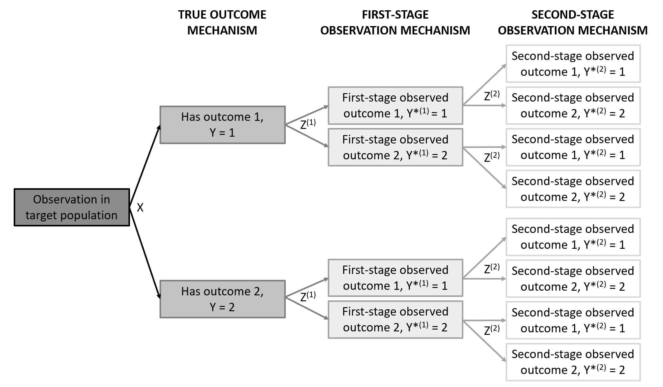
Figure 1: Diagram of the assumed data structure for a two-stage misclassification model.

We define the probability of observing outcomes $\mathscr{k}^{(a)}$ in stage $a$ of the model using the model structure

$$P(Y^{*(a)}=k^{(a)}) \;=\sum_{j=1}^{2}\sum_{k^{(a-1)},\dots,k^{(1)}=1}^{2}\Bigl{(}P(Y^{*(a)}=k^{(a)}|\mathcal{Y}^{*(a-1)},Y=j,Z^{(a)},\dots,Z^{(1)};\gamma)$$ (3)

$$\qquad\phantom{a}\times P(Y^{*(a-1)}=k^{(a-1)}|\mathcal{Y}^{*(a-2)},Y=j,Z^{(a-1)},\dots,Z^{(1)};\gamma)\times\dots$$

$$\qquad\phantom{a}\times P(Y^{*(1)}=k^{(1)}|Y=j,Z^{(1)};\gamma)\times P(Y=j|X;\beta)\Bigr{)}$$

$$=\sum_{j=1}^{2}\sum_{k^{(a-1)},\dots,k^{(1)}=1}^{2}\Bigl{(}\pi^{*(a)}_{\mathscr{k}^{(a)}j}\times\pi^{*(a-1)}_{\mathscr{k}^{(a-1)}j}\times\dots\times\pi^{*(1)}_{\mathscr{k}^{(1)}j}\times\pi_{ij}\Bigr{)}.$$

The contribution to the likelihood by a single subject $i$ is thus $\prod_{k^{(a)}=1}^{2}P(Y_{i}^{*(a)}=k^{(a)})^{y^{*(a)}_{ik^{(a)}}}$ where $y^{*(a)}_{ik^{(a)}}=\mathbb{I}\{Y_{i}^{*(a)}=k^{(a)}\}$. We can estimate $(\beta,\gamma)$ using the following observed data log-likelihood for subjects $i=1,\dots,N$,

$$\ell_{obs}(\beta,\gamma;X,Z^{(a)},\dots,Z^{(1)}) \;=\sum_{i=1}^{N}\log\Bigl{\{}\prod_{b=1}^{a}\bigl{(}\prod_{k^{(b)}=1}^{2}P(Y_{i}^{*(b)}=k^{(b)})^{y^{*(b)}_{ik^{(b)}}}\bigr{)}\Bigr{\}}$$ (4)

$$=\sum_{i=1}^{N}\Bigl{[}\sum_{b=1}^{a}y^{*(b)}_{ik^{(b)}}\sum_{k^{(b)}=1}^{2}\log\{P(Y_{i}^{*(b)}=k^{(b)})\}\Bigr{]}$$

$$=\sum_{i=1}^{N}\Bigl{[}\sum_{b=1}^{a}y^{*(b)}_{ik^{(b)}}\sum_{k^{(b)}=1}^{2}\log\{\sum_{j=1}^{2}\sum_{k^{(b-1)},\dots,k^{(1)}=1}^{2}\bigl{(}\pi^{*(b)}_{\mathscr{k}^{(b)}j}\times\pi^{*(b-1)}_{\mathscr{k}^{(b-1)}j}\times\dots\times\pi^{*(1)}_{\mathscr{k}^{(1)}j}\times\pi_{ij}\bigr{)}\}\Bigr{]}$$

where $\sum_{k^{(a)},\dots,k^{(1)}=1}^{2}$ is equivalent to $\sum_{k^{(a)}=1}^{2},\sum_{k^{(a-1)}=1}^{2},\dots,\sum_{k^{(1)}=1}^{2}$. As in the basic model, the observed data log-likelihood is difficult to use directly for optimization. Instead, we can view the true outcome $Y$ as a latent variable, and construct the complete data log-likelihood for a multistage model as follows,

$$\ell_{complete}(\beta,\gamma;X,Z^{(a)},\dots,Z^{(1)}) \;=\sum_{i=1}^{N}\Bigl{[}\sum_{j=1}^{2}y_{ij}\text{log}\{P(Y_{i}=j|X_{i})\}$$ (5)

$$+\sum_{b=1}^{a}\Bigl{(}\sum_{j=1}^{2}\sum_{k^{(a)},\dots,k^{(1)}=1}^{2}y_{ij}\bigl{(}\prod_{h=1}^{b}y^{*(h)}_{ik^{(h)}}\bigr{)}\text{log}\{P(Y^{*(b)}_{i}=k^{(b)}|\mathcal{Y}^{*(b-1)},Y=j,Z^{(b)})\}\Bigr{)}\Bigr{]}$$

$$=\sum_{i=1}^{N}\Bigl{[}\sum_{j=1}^{2}y_{ij}\text{log}\{\pi_{ij}\}+\sum_{b=1}^{a}\Bigl{(}\sum_{j=1}^{2}\sum_{k^{(a)},\dots,k^{(1)}=1}^{2}y_{ij}\bigl{(}\prod_{h=1}^{b}y^{*(h)}_{ik^{(h)}}\bigr{)}\text{log}\{\pi^{*(b)}_{i\mathscr{k}^{(b)}j}\}\Bigr{)}\Bigr{]}.$$

Since we do not observe the true outcome value $Y$, the complete data log-likelihood cannot be used for maximization. Note that (5) can be viewed as a mixture model with latent mixture components, $y_{ij}$, and covariate-dependent mixing proportions $\pi_{ij}$.

Since the complete data log-likelihood for the multistage model is a mixture likelihood, it is also invariant under relabeling of the mixture components, $y_{ij}$. Regardless of the number of stages in the model, $a$, there are two mixture components and therefore $J!=2!=2$ plausible parameter sets (Betancourt,, 2017; Stephens,, 2000). In addition, the pattern that governs these parameter sets is identical to that described in Webb and Wells, (2023), the $\beta$ parameters change signs and the $\gamma$ parameters change $j$ subscripts. A procedure to correct label switching in a multistage misclassification model is provided in Algorithm 1 (Webb and Wells,, 2023).

Algorithm 1 Correcting label switching in multistage binary outcome misclassification models

Compute average $\pi^{*(b)}_{\mathscr{k}^{(b)}=j,j}=\pi^{*(b)}_{k^{(b)}=j,k^{(b-1)}=j,\dots,k^{(1)}=j,j}$ for all $j\in\{1,2\}$ and all $b\in\{1,\dots,a\}$ using $\hat{\beta}$ and $\hat{\gamma}$.

if $\pi^{*(b)}_{\mathscr{k}^{(b)}=j,j}>0.50$ for all $j\in\{1,2\}$ and all $b\in\{1,\dots,a\}$ then

     $\hat{\beta}_{corrected}\leftarrow\hat{\beta}$

     $\hat{\gamma}_{corrected}\leftarrow\hat{\gamma}$

else

     $\hat{\beta}_{corrected}\leftarrow-\hat{\beta}$

     $\hat{\gamma}^{(b)}_{corrected,\mathscr{k}^{(b)}1}\leftarrow\hat{\gamma}^{(b)}_{\mathscr{k}^{(b)}2}$

     $\hat{\gamma}^{(b)}_{corrected,\mathscr{k}^{(b)}2}\leftarrow\hat{\gamma}^{(b)}_{\mathscr{k}^{(b)}1}$

end if

Algorithm 1 relies on the following identification assumption:

Assumption 1

The probability of correct classification is at least 0.50, on average across subjects $i$ and across all model stages; that is, $\pi^{*(a)}_{\mathscr{k}^{(a)}=j,j}=\pi^{*(a)}_{k^{(a)}=j,k^{(a-1)}=j,\dots,k^{(1)}=j,j}>0.50$.

Note that Algorithm 1 uses average conditional response probabilities for all observation stages $b\in\{1,\dots,a\}$. Depending on the problem context, analysts may instead choose to implement Algorithm 1 using average conditional response probabilities from only a subset of the model stages. This choice would create a less strict criterion for label switching, but would be simpler to implement than if all $a$ stage outcomes were considered.

3.1 Estimation Methods

Both the EM algorithm and MCMC can be used to estimate $\beta$ and $\gamma$ in a multistage misclassification model. Both estimation strategies are available in the R Package COMBO for a two-stage misclassification model (Hochstedler,, 2023).

3.1.1 Maximization Using an EM Algorithm

Because 5 is linear in $y_{ij}$, we can replace $y_{ij}$ with the following quantity in the E-step of the algorithm,

$$w^{(a)}_{ij}=P(Y_{i}=j|Y_{i}^{*(a)},\dots,Y_{i}^{*(1)},X,Z)=\sum_{k^{(a)},\dots,k^{(1)}=1}^{2}\frac{\pi_{ij}\bigl{(}\prod_{b=1}^{a}y^{*(b)}_{ik^{(b)}}\pi^{*(b)}_{i\mathscr{k}^{(b)}j}\bigr{)}}{\sum_{\ell=1}^{2}\pi_{i\ell}\bigl{(}\prod_{b=1}^{a}\pi^{*(b)}_{i\mathscr{k}^{(b)}\ell}\bigr{)}}.$$ (6)

In the M-step, we maximize the following expected log-likelihood with respect to $\beta$ and $\gamma$,

$$Q=\sum_{i=1}^{N}\Bigl{[}\sum_{j=1}^{2}w^{(a)}_{ij}\text{log}\{\pi_{ij}\}+\sum_{b=1}^{a}\Bigl{(}\sum_{j=1}^{2}\sum_{k^{(a)},\dots,k^{(1)}=1}^{2}w^{(a)}_{ij}\bigl{(}\prod_{h=1}^{b}y^{*(h)}_{ik^{(h)}}\bigr{)}\text{log}\{\pi^{*(b)}_{i\mathscr{k}^{(b)}j}\}\Bigr{)}\Bigr{]}.$$ (7)

After estimates for $\beta$ and $\gamma$ are obtained from this EM algorithm, Algorithm 1 must be used to correct potential label switching and return final parameter estimates. The covariance matrix for $\beta$ and $\gamma$ is obtained by inverting the expected information matrix.

3.1.2 Bayesian Modeling

Our proposed multistage misclassification model is defined for each of the $a$ stages in the model: $Y^{*(a)}_{ik^{(a)}}|\pi^{*(a)}_{ik^{(a)}}\sim Multinomial(\pi^{*(a)}_{ik^{(a)}},J)$. Here, $\pi^{*(a)}_{ik^{(a)}}=\sum_{j=1}^{2}\sum_{k^{(a-1)},\dots,k^{(1)}=1}^{2}\pi^{*(a)}_{i\mathscr{k}^{(a)}j}\times\pi^{*(a-1)}_{i\mathscr{k}^{(a-1)}j}\times\dots\times\pi^{*(1)}_{i\mathscr{k}^{(1)}j}\times\pi_{ij}$. $J$ refers to the number of outcome categories. Prior distributions for the parameters should be determined using input from subject-matter experts, based on the context of the problem that the model is applied to. We recommend proper, relatively flat priors. In the R Package, COMBO, users can specify prior parameters for either Uniform, Normal, Double Exponential, or t prior distributions. Before summarizing the results, Algorithm 1 must be applied on each individual MCMC chain to correct for label switching, if it is present. Standard methods are used to compute variance metrics.

4 Simulation Studies

We present simulations for evaluating the proposed binary outcome misclassification model in terms of bias and root mean squared error (rMSE) for two-stage cases. The two-stage mislcassification model is compared to a naive two-stage model that assumes no measurement error in both of the observed outcomes.

We investigate four simulation settings with varying sample sizes and misclassification rates: (1) small sample size and large misclassification rates and (2) large sample size and small misclassification rates, (3) small sample size and perfect $Y^{*(1)}$ and, (4) small sample size and perfect specificity in $Y^{*(2)}$. We present results from the EM algorithm for settings 1-4 and results from MCMC for settings 1, 3, and 4. MCMC was not performed for setting 2 due to computational time constraints (see Appendix A). Details on these settings can be found in Appendix A.

Table 1 and Table 2 present mean parameter estimates and rMSE across 500 simulated datasets for simulation settings 1-4. For each simulation setting, Table 3 presents the true outcome probability, first-stage sensitivity, first-stage specificity, second-stage sensitivity, and second-stage specificity values measured from the generated data and estimated from the EM algorithm and MCMC results.

Table 1: Bias and root mean squared error (rMSE) for parameter estimates from 500 realizations of simulation Settings 1 and 2. “EM” and “MCMC” estimates were computed using the COMBO R Package. The “Naive Analysis” results were obtained by a two-stage model that does not account for outcome misclassification. Estimates marked with a “-” are not obtained by the given estimation method.

		EM		MCMC		Naive Analysis
Scenario		Bias	rMSE	Bias	rMSE	Bias	rMSE
	$\beta_{0}$	0.032	0.197	-0.053	0.224	0.029	0.299
(1)	$\beta_{X}$	-0.101	0.301	0.261	0.490	-0.100	0.547
	$\gamma^{(1)}_{110}$	-0.028	0.209	0.249	0.522	-	-
	$\gamma^{(1)}_{11Z^{(1)}}$	0.044	0.338	0.405	1.046	-	-
	$\gamma^{(1)}_{120}$	0.067	0.333	-0.496	1.210	-	-
	$\gamma^{(1)}_{12Z^{(1)}}$	-0.156	0.656	-1.425	2.168	-	-
	$\gamma^{(2)}_{1110}$	-0.014	0.249	1.697	2.385	-0.195	0.364
	$\gamma^{(2)}_{111Z^{(2)}}$	0.047	0.374	2.674	2.989	0.114	1.233
	$\gamma^{(2)}_{1210}$	-0.022	0.652	-2.938	4.341	-	-
	$\gamma^{(2)}_{121Z^{(2)}}$	0.128	0.710	2.674	3.664	-	-
	$\gamma^{(2)}_{1120}$	0.017	1.236	2.387	3.925	-	-
	$\gamma^{(2)}_{112Z^{(2)}}$	-0.398	3.091	-0.124	3.091	-	-
	$\gamma^{(2)}_{1220}$	0.026	0.343	-1.918	2.647	-0.073	3.909
	$\gamma^{(2)}_{122Z^{(2)}}$	-0.125	0.581	-3.025	3.247	-0.390	3.251
	$\beta_{0}$	0.003	0.036			0.006	0.058
(2)	$\beta_{X}$	-0.005	0.062			0.026	0.101
	$\gamma^{(1)}_{110}$	-0.011	0.108			-	-
	$\gamma^{(1)}_{11Z^{(1)}}$	0.013	0.096			-	-
	$\gamma^{(1)}_{120}$	0.036	0.188			-	-
	$\gamma^{(1)}_{12Z^{(1)}}$	-0.035	0.213			-	-
	$\gamma^{(2)}_{1110}$	-0.012	0.111			-0.053	0.157
	$\gamma^{(2)}_{111Z^{(2)}}$	0.013	0.108			-0.128	0.208
	$\gamma^{(2)}_{1210}$	0.166	0.413			-	-
	$\gamma^{(2)}_{121Z^{(2)}}$	-0.061	0.211			-	-
	$\gamma^{(2)}_{1120}$	-0.110	0.492			-	-
	$\gamma^{(2)}_{112Z^{(2)}}$	0.024	0.234			-	-
	$\gamma^{(2)}_{1220}$	-0.027	0.151			-0.092	0.239
	$\gamma^{(2)}_{122Z^{(2)}}$	0.006	0.133			0.234	0.363

Table 2: Bias and root mean squared error (rMSE) for parameter estimates from 500 realizations of simulation Settings 3 and 4. “EM” and “MCMC” estimates were computed using the COMBO R Package. The “Naive Analysis” results were obtained by a two-stage model that does not account for outcome misclassification. Estimates marked with a “-” are not obtained by the given estimation method.

		EM		MCMC		Naive Analysis
Scenario		Bias	rMSE	Bias	rMSE	Bias	rMSE
	$\beta_{0}$	-0.018	0.118	-0.001	0.113	0.016	0.247
(3)	$\beta_{X}$	-0.097	0.195	0.013	0.166	-0.131	0.457
	$\gamma_{110}$	19.373	65.503	1.26	1.640	-	-
	$\gamma_{11Z^{(1)}}$	-4.068	14.446	-0.450	1.094	-	-
	$\gamma_{120}$	-43.863	186.594	-0.815	1.397	-	-
	$\gamma_{12Z^{(1)}}$	-4.388	285.955	0.678	1.295	-	-
	$\gamma^{(2)}_{1110}$	-0.016	0.194	-0.033	0.327	-0.034	0.325
	$\gamma^{(2)}_{111Z^{(2)}}$	0.064	0.282	0.527	0.969	0.239	0.898
	$\gamma^{(2)}_{1210}$	1.247	2.059	-0.797	1.084	-	-
	$\gamma^{(2)}_{121Z^{(2)}}$	1.224	2.035	-0.742	1.049	-	-
	$\gamma^{(2)}_{1120}$	2.191	2.820	0.872	1.236	-	-
	$\gamma^{(2)}_{112Z^{(2)}}$	1.727	2.242	0.345	0.883	-	-
	$\gamma^{(2)}_{1220}$	0.000	0.228	-0.006	0.631	-0.024	2.788
	$\gamma^{(2)}_{122Z^{(2)}}$	-0.082	0.335	-1.019	1.589	-0.968	6.350
	$\beta_{0}$	0.016	0.165	-0.049	0.230	0.006	0.232
(4)	$\beta_{X}$	-0.160	0.266	0.037	0.272	-0.149	0.349
	$\gamma_{110}$	-0.057	0.197	0.101	0.293	-	-
	$\gamma_{11Z^{(1)}}$	0.061	0.264	0.211	0.749	-	-
	$\gamma_{120}$	0.133	0.282	0.017	0.458	-	-
	$\gamma_{12Z^{(1)}}$	-0.042	0.440	-0.655	1.292	-	-
	$\gamma^{(2)}_{1110}$	0.011	0.252	1.119	1.823	-0.195	0.349
	$\gamma^{(2)}_{111Z^{(2)}}$	0.034	0.394	1.888	2.381	0.033	1.549
	$\gamma^{(2)}_{1210}$	-0.114	0.509	-2.304	4.178	-	-
	$\gamma^{(2)}_{121Z^{(2)}}$	0.004	0.461	2.610	3.502	-	-
	$\gamma^{(2)}_{1120}$	-0.067	9.275	-0.134	1.197	-	-
	$\gamma^{(2)}_{112Z^{(2)}}$	1.251	8.798	1.370	2.132	-	-
	$\gamma^{(2)}_{1220}$	-12.413	29.590	-1.238	1.365	-4.833	18.441
	$\gamma^{(2)}_{122Z^{(2)}}$	-9.996	24.390	0.413	0.731	3.482	10.316

Table 3: Estimated event probabilities from 500 realizations of simulation Settings 1-4. “Data” terms refer to empirical values computed from generated datasets. “EM” and “MCMC” estimates were computed using the COMBO R Package.

Scenario			Data	EM	MCMC
(1)		$P(Y=1)$	0.648	0.647	0.650
		$P(Y=2)$	0.352	0.353	0.350
		$P(Y^{*(1)}=1|Y=1)$	0.852	0.848	0.888
		$P(Y^{*(1)}=2|Y=2)$	0.822	0.816	0.897
		$P(Y^{*(2)}=1|Y^{*(1)}=1,Y=1)$	0.903	0.901	0.978
		$P(Y^{*(2)}=2|Y^{*(1)}=2,Y=2)$	0.853	0.851	0.973
(2)		$P(Y=1)$	0.648	0.648
		$P(Y=2)$	0.352	0.352
		$P(Y^{*(1)}=1|Y=1)$	0.921	0.920
		$P(Y^{*(1)}=2|Y=2)$	0.921	0.919
		$P(Y^{*(2)}=1|Y^{*(1)}=1,Y=1)$	0.949	0.949
		$P(Y^{*(2)}=2|Y^{*(1)}=2,Y=2)$	0.920	0.921
(3)		$P(Y=1)$	0.647	0.640	0.648
		$P(Y=2)$	0.353	0.360	0.352
		$P(Y^{*(1)}=1|Y=1)$	1	0.997	0.999
		$P(Y^{*(1)}=2|Y=2)$	1	0.977	0.999
		$P(Y^{*(2)}=1|Y^{*(1)}=1,Y=1)$	0.902	0.903	0.917
		$P(Y^{*(2)}=2|Y^{*(1)}=2,Y=2)$	0.851	0.855	0.890
(4)		$P(Y=1)$	0.648	0.642	0.641
		$P(Y=2)$	0.352	0.358	0.359
		$P(Y^{*(1)}=1|Y=1)$	0.851	0.847	0.871
		$P(Y^{*(1)}=2|Y=2)$	0.820	0.803	0.848
		$P(Y^{*(2)}=1|Y^{*(1)}=1,Y=1)$	0.903	0.903	0.967
		$P(Y^{*(2)}=2|Y^{*(1)}=2,Y=2)$	1	0.994	0.999

Setting 1: Across all simulated datasets, the average $P(Y=1)$ was $64.8\%$, the average $P(Y^{*(1)}=1)$ was $61.5\%$, and the average $P(Y^{*(2)}=1)$ was $63.3\%$. The average first-stage correct classification rate was $85.2\%$ for $Y^{*(1)}=1$ and $82.2\%$ for $Y^{*(1)}=2$. The average second-stage correct classification rate was $90.3\%$ for $Y^{*(2)}=1$ and $85.3\%$ for $Y^{*(2)}=2$ (Table 3). The naive analysis results in small bias for $\beta_{X}$, but the rMSE is large compared to the EM Algorithm and MCMC methods that account for potential misclassification (Table 1). Our proposed EM Algorithm performs well for the $\beta$ parameters and first-stage $\gamma$ parameters. Some of the second-stage $\gamma$ parameter estimates have wider variation. While our proposed MCMC method performs well for the $\beta$ parameter estimates, the bias and rMSE for the $\gamma$ estimates are considerably higher than that of the EM Algorithm. Both the EM Algorithm and MCMC methods recover the true outcome probabilities $P(Y=1)$ and $P(Y=2)$ in Table 3, but MCMC tends to consistently overestimate correct classification rates for both stages of model.

Setting 2: In Setting 2, the average $P(Y=1)$ was $64.8\%$ (Table 3). The observed outcome response probabilities were $62.4\%$ for $Y^{*(1)}$ and $64.4\%$ for $Y^{*(2)}$. The average first-stage sensitivity and specificity were both $92.1\%$. For second-stage outcomes, the average correct classification rate was $94.9\%$ for $Y^{*(2)}=1$ and $92.0\%$ for $Y^{*(2)}=2$. While the bias for naive $\beta$ estimates is not large, the naive method rMSE is higher than that of the two-stage misclassification model (Table 1). The two-stage misclassification model achieves low bias across all parameter estimates using the EM Algorithm. In addition the EM Algorithm results in near-perfect recovery of response probabilities and conditional response probabilities for $Y$, $Y^{*(1)}$, and $Y^{*(2)}$ (Table 3). It should be noted that there were numerical issues in the estimation of many realizations for Setting 5. Scaling this method to large sample sizes is a topic under investigation.

Setting 3: In Setting 3, the average response probabilities for each marginal outcome, $Y$, $Y^{*(1)}$, and $Y^{*(2)}$ were $64.7\%$, $64.7\%$, and $63.6\%$, respectively. Per the simulation design, $Y^{*(1)}$ was measured without error. The second-stage correct classification rate was $90.2\%$ for $Y^{*(2)}=1$ and $85.1\%$ for $Y^{*(2)}=2$ (Table 3). In this setting, the naive model is an appropriate choice for the data. As such, we find low bias in the naive $\beta$ estimates in Table 2. Across both the EM Algorithm and MCMC estimates, we find substantial bias and large rMSE estimates for the first-stage $\gamma$ parameters. This is not concerning, since the first-stage $\gamma$ parameters govern the misclassification mechanism for $Y^{*(1)}$, and there is no first-stage misclassification in the design. Similarly, the second-stage $\gamma$ parameters associated with mismatched $Y$ and $Y^{*(1)}$ terms are estimated with considerable bias using both the EM Algorithm and MCMC. Since mismatched $Y$ and $Y^{*(1)}$ terms are not possible in this study design, it is unsurprising that the corresponding regression parameters are estimated poorly. The remaining second-stage $\gamma$ terms, however, are estimated with low bias and with rMSE well under the naive model using the EM Algorithm. MCMC also produces reasonable estimates, but the bias and rMSE are both higher than that of the EM Algorithm. In Table 3, we see that both the EM and MCMC methods provide accurate estimates of $Y$ response probabilities. Importantly, both methods also correctly capture the perfect measurement of $Y^{*(1)}$, with correct classification probabilities estimated between $97.7\%$ and $99.9\%$. Second-stage correct classification rates are also estimated accurately using the EM Algorithm. These probabilities are slightly overestimated using MCMC.

Setting 4: In Setting 4, the average response probability for $Y=1$ was $64.8\%$ (Table 3). The average response probabilities for the first-stage and second-stage observed outcomes were $61.5\%$ and $56.7\%$, respectively. The average first-stage correct classification rate was $85.1\%$ for $Y^{*(1)}=1$ and $82.0\%$ for $Y^{*(1)}=2$. The average second-stage correct classification rate was $90.3\%$ for $Y^{*(2)}=1$. Per the simulation design, $P(Y^{*(2)}|Y^{*(1)}=2,Y=2)=1$. The naive analysis yields low bias for $\beta$ terms and for $\gamma^{(2)}_{111}$ terms, but the rMSE is higher than that of the EM Algorithm estimates, in particular (Table 2). The EM algorithm performs well in terms of bias and rMSE for most terms, but estimation is problematic for $\gamma^{(2)}_{1220}$ and $\gamma^{(2)}_{122Z^{(2)}}$. These results are not concerning because extreme parameter estimates correspond to a lack of misclassification in the specificity mechanism of the second-stage outcomes, which was appropriate given the simulation design. The MCMC estimation did not show this extreme behavior in the estimates of $\gamma^{(2)}_{1220}$ and $\gamma^{(2)}_{122Z^{(2)}}$, presumably due to the limits of the uniform prior distribution used in the analysis. For other terms in the model, MCMC also produced reasonable estimates, though bias and rMSE were generally higher than that of the EM algorithm, especially for second-stage $\gamma^{(2)}$ parameters. Both the EM Algorithm and MCMC estimates correspond to highly accurate estimates of response and first-stage classification probabilities $P(Y=1)$, $P(Y^{*(1)}=1|Y=1)$, and $P(Y^{*(1)}=2|Y=2)$ (Table 3). The EM Algorithm estimates $P(Y^{*(2)}=1|Y^{*(1)}=1,Y=1)$ without bias, while MCMC overestimates the quantity. Importantly, both methods correctly estimate near-perfect classification for $P(Y^{*(2)}=2|Y^{*(1)}=2,Y=2)$, as specified by the simulation design.

5 Evaluating the Accuracy of Pretrial Assessments and Judicial Decisions

In this section, we apply our model to investigate risk factors for reoffense or FTA in the presence of two sequential and dependent noisy outcomes: VPRAI recommendations and judge decisions.

Our first stage response variable is the VPRAI recommendation, dichotomized into “detain” and “release” recommendation categories. Our second-stage response variable is the court’s final decision to detain or release a defendant before their trial. We assessed the association of pretrial failure with risk factors including the number of prior failures to appear (FTA) for trial, employment status, drug abuse history, and the number of previous violent arrests. Employment and drug history variables were coded as binary indicators.

We estimated model parameters using the EM algorithm and label switching correction for the multistage model, defined in Section 3. Parameter estimates and standard errors are provided in Table 4. With the exception of the intercept and drug history association parameters, the $\beta$ estimates in the misclassification model are all attenuated compared to the naive model. We find that increased numbers of previous FTA, unemployment, a history of drug abuse, and increased numbers of violent arrests are all associated with true incidence of recidivism or FTA in this data set. For the first-stage outcome, we find that, given true recidivism or FTA, Black defendants are more likely to have a VPRAI detention recommendation than white defendants. Moreover, given no reoffense or FTA, Black defendants are still more likely to have a VPRAI detention recommendation than white defendants. This trend remains for court decisions. Given no pretrial failure and regardless of VPRAI recommendations, Black individuals are more likely to be detained by the court than white individuals. Similarly, given pretrial failure and a VPRAI detention recommendation, Black defendants are more likely to be detained before their trial than white defendants. Black defendants are also more likely to be detained before their trial than white defendants in the case of true recidivism or FTA and a VPRAI recommendation of “release”, though this parameter estimate has extremely high standard error due to perfect separation, or perfect prediction of the outcome by race (Mansournia et al.,, 2018). In fact, conditional on true recidivism or FTA and a VPRAI “release” recommendation, our model estimates that $100\%$ of Black defendants are detained by judges.

Table 4: Parameter estimates and standard errors from the applied example using the Virginia Department of Criminal Justice Services dataset.“EM” estimates were computed using the COMBO R Package. The “Naive Analysis” results were obtained by running a two-stage model that does not account for outcome misclassification. Estimates marked with a “-” are not obtained by the given estimation method. $\beta_{FTA}$ refers to the association between a defendant’s number of previous failures to appear (FTA) and recidivism. $\beta_{unemployed}$ refers to the association between employment status (reference = employed or unable to work) and recidivism. $\beta_{drug}$ refers to the association between drug abuse history (reference = no history of drug abuse) and recidivism. $\beta_{violent}$ refers to the association between a defendant’s number of previous violent arrests and recidivism. $\gamma^{(1)}_{1,j,race}$ refers to the association between race and VPRAI risk score, given true recidivism status $j$. $\gamma^{(2)}_{1,k,j,race}$ refers to the association between race and the court’s decision to detain a defendant, given VPRAI risk score $k$ and true recidivism status $j$. The reference category for race is white. $\beta_{0}$, $\gamma^{(1)}_{1j0}$, and $\gamma^{(2)}_{1kj0}$ are intercept terms for all $j$ and all $k$.

		EM		Naive Analysis
		Est.	SE	Est.	SE
$\beta_{0}$		-3.512	0.105	-2.382	1.943
$\beta_{FTA}$		1.224	0.218	1.344	1.328
$\beta_{unemployed}$		0.732	0.056	1.036	1.094
$\beta_{drug}$		1.968	0.126	1.586	1.251
$\beta_{violent}$		0.280	0.0223	1.028	1.328
$\gamma^{(1)}_{110}$		-0.029	0.199	-	-
$\gamma^{(1)}_{11,race}$		1.843	0.376	-	-
$\gamma^{(1)}_{120}$		-20.270	0.605	-	-
$\gamma^{(1)}_{12,race}$		15.341	0.603	-	-
$\gamma^{(2)}_{1110}$		1.576	0.298	0.666	0.296
$\gamma^{(2)}_{111,race}$		0.327	0.374	0.364	0.230
$\gamma^{(2)}_{1210}$		0.892	0.203	-	-
$\gamma^{(2)}_{121,race}$		15.645	182.618	-	-
$\gamma^{(2)}_{1120}$		-6.492	1.858	-	-
$\gamma^{(2)}_{112,race}$		9.822	1.859	-	-
$\gamma^{(2)}_{1220}$		-0.418	0.018	-0.668	0.304
$\gamma^{(2)}_{122,race}$		0.459	0.018	0.517	0.171

We also use the EM Algorithm parameter estimates to assess VPRAI sensitivity and specificity, as well as the fairness and accuracy of judge decisions. In the sample, we estimate a pretrial failure rate of $17.9\%$. The VPRAI appears to have moderate sensitivity and near-perfect specificity; we estimate that the VPRAI correctly recommends detention for $67.5\%$ of defendants and correctly recommends release for $99.6\%$ of defendants. This sensitivity rate, however, differs by defendant race. Among Black defendants who are expected to reoffend or fail to appear for their trial date, the VPRAI recommends pretrial detention $86.0\%$ of the time. Among white defendants, this rate drops to just $49.3\%$. Moving to judge decisions, we estimate that, among individuals who had a VPRAI detention recommendation, judges correctly detain defendants in $84.9\%$ of cases. However, among defendants who received a VPRAI release recommendation, we estimate that judges correctly release defendants just $54.7\%$ of the time. Again, these rates differ by defendant race. Among defendants estimated to truly reoffend or not appear for trial and who were given a VPRAI detention recommendation, a court detention decision is received by $82.9\%$ of white defendants and $87.0\%$ of Black defendants. Among white defendants who are not expected to reoffend or fail to appear and who have VPRAI “release” recommendations, we estimate that $60.3\%$ are, in fact, released before their trial. Among Black defendants, this proportion drops to just $49.0\%$. Collapsing across VPRAI recommendations, we estimate that judges appropriately detain white individuals in $76.8\%$ of cases and appropriately detain Black individuals in $88.8\%$ of cases, suggesting that white defendants may be given “the benefit of the doubt” more often than Black defendants. Similarly, we estimate that white defendants are wrongfully detained by the court in $39.7\%$ of cases, but wrongful detentions happen in as many as $51.4\%$ of cases involving Black defendants.

6 Discussion

In this work, we assess the accuracy of pretrial risk assessment recommendations and judicial decisions in predicting defendant pretrial failure and find that Black defendants are more often misclassified—both by the VPRAI and, to a greater extent, judicial officers—relative to their white counterparts. Practically, this means that, conditioned on the likelihood of pretrial failure, the VPRAI more often recommends detention for Black defendants, and that judges are more likely to detain Black defendants, regardless of VPRAI recommendation or likelihood of pretrial failure. This suggests that pretrial risk assessments may actually institutionalize or exacerbate the very racial inequality they are intended to combat. These results have implications not only for Virginia, but also for every jurisdiction that administers pretrial risk assessments.

Beyond this specific application, our algorithm has a wide array of use cases in other high-stakes policy settings. Many public sector algorithms estimate binary outcomes to aid human decision-making, including child welfare intervention systems (Chouldechova et al.,, 2018), welfare fraud detection algorithms (Eubanks,, 2018), and public housing allocation systems (Balagot et al.,, 2019; Schneider,, 2020). The decisions these algorithms and agencies make can change the course of a person’s life. Our algorithm offers a method of exposing instances of misclassification that may systematically disadvantage certain groups of people. While similar approaches of measuring such disparities exist, they require known misclassification rates and perfect sensitivity (Fogliato et al.,, 2020), or only account for only a single observed proxy (Webb and Wells,, 2023). Our methods have the additional strengths of not requiring gold standard labels and of being a multi-stage generalization of the work of Webb and Wells, (2023). Specifically, we can handle data generation processes that are comprised of multiple dependent and sequential misclassified binary outcomes.

Further generalizations of our methods are still possible in future work. For example, our work assumes that predictor variables are correctly measured, which is unlikely in practice. A more complex modeling structure would be required to account for imperfect arrest records or demographic variables. In addition, our method is limited to sequential and dependent binary outcomes. If categorical or continuous outcomes are present in a research design, further extensions of this work would be required.

Acknowledgements

The authors would like to thank Karen Levy and Solon Barocas for their insights into pretrial detention processes. Data used in the two-stage misclassification model analysis was provided by the Virginia Department of Criminal Justice Services.

Funding

Funding support for Kimberly A. H. Webb was provided by the LinkedIn and Cornell Ann S. Bowers College of Computing and Information Science strategic partnership PhD Award. Martin T. Wells was supported by NIH awards U19AI111143-07 and P01-AI159402.

Disclosure Statement

The authors report there are no competing interests to declare.

Appendix A Simulation Study Settings

A.1 Simulation Settings

We present simulations for evaluating the proposed binary outcome misclassification model in terms of bias and root mean squared error (rMSE) for two-stage cases. For a given simulation scenario, we present parameter estimates for a binary outcome misclassification model obtained from the EM-algorithm and from MCMC, under a Uniform$(-10,10)$ prior distribution setting. We compare our estimates to a naive analysis model that assumes $Y^{*(1)}$ and $Y^{*(2)}$ are measured without error.

In all settings, we generate $500$ datasets with $P(Y=1)\approx 65\%$. In the simulation settings for the two-stage model, we consider four simulation scenarios. First, we examine the case of a relatively small sample size and high misclassification rate, as this case would likely be highly problematic in a two-stage example. In this setting, datasets had $1000$ members and the imposed outcome misclassification rates for $Y^{*(1)}$ were between $10\%$ and $22\%$. The probability of correct measurement across all stages was set between $79\%$ and $92\%$. In Setting 2, we show that even with two sequential observed outcomes and a large sample size, even small misclassification rates can still impact parameter estimation. In this setting, we generated datasets with $10000$ members and imposed misclassification rates in $Y^{*(1)}$ between $4\%$ and $9\%$. In the third simulation setting, we evaluated the case where $Y^{*(1)}$ is measured without error, but $Y^{*(2)}$ is subject to misclassification. In Setting 4, we instead consider the case where $Y^{*(1)}$ is subject to misclassification, but $Y^{*(2)}$ has perfect specificity. These scenarios demonstrate that our multistage methods are still appropriate for cases where there is perfect measurement in at least one of the observed outcomes. In both Setting 3 and Setting 4, we generated datasets with $1000$ members and imposed misclassification rates between $10\%$ and $20\%$ in the imperfectly measured outcome.

For a dataset with $1,000$ members, the two-stage analysis using our proposed EM algorithm took about $25$ seconds. The MCMC analysis took considerably longer, at approximately $3.5$ hours.

These settings are outlined in Table 5. All analyses were conducted in R (R Core Team,, 2021).

Table 5: Number of generated datasets (N. Realizations), Sample size ($N$), $P(Y=1)$, first-stage sensitivity ($P(Y^{*}=1|Y=1)$), first-stage specificity ($P(Y^{*}=2|Y=2)$), second-stage sensitivity ($P(Y^{*(2)}=1|Y^{*(1)}=1,Y=1)$), second-stage specificity ($P(Y^{*(2)}=2|Y^{*(1)}=2,Y=2)$), $\beta$ prior distribution, and $\gamma$ prior distribution settings for each of the the simulation Settings 4, 5, and 6.

Scenario				Setting
(1)		N. Realizations		500
		$N$		1000
		$P(Y=1)$		0.65
		$P(Y^{*(1)}=1|Y=1)$		0.83 - 0.91
		$P(Y^{*(1)}=2|Y=2)$		0.79 - 0.85
		$P(Y^{*(2)}=1|Y^{*(1)}=1,Y=1)$		0.85 - 0.92
		$P(Y^{*(2)}=2|Y^{*(1)}=2,Y=2)$		0.79 - 0.87
		$\beta$ prior distribution		Uniform$(-10,10)$
		$\gamma$ prior distribution		Uniform$(-10,10)$
(2)		N. Realizations		500
		$N$		10000
		$P(Y=1)$		0.65
		$P(Y^{*(1)}=1|Y=1)$		0.91 - 0.93
		$P(Y^{*(1)}=2|Y=2)$		0.91 - 0.93
		$P(Y^{*(2)}=1|Y^{*(1)}=1,Y=1)$		0.94 - 0.96
		$P(Y^{*(2)}=2|Y^{*(1)}=2,Y=2)$		0.91 - 0.93
		$\beta$ prior distribution		Uniform$(-10,10)$
		$\gamma$ prior distribution		Uniform$(-10,10)$
(3)		N. Realizations		500
		$N$		1000
		$P(Y=1)$		0.65
		$P(Y^{*(1)}=1|Y=1)$		1
		$P(Y^{*(1)}=2|Y=2)$		1
		$P(Y^{*(2)}=1|Y^{*(1)}=1,Y=1)$		0.88 - 0.92
		$P(Y^{*(2)}=2|Y^{*(1)}=2,Y=2)$		0.82 - 0.90
		$\beta$ prior distribution		Uniform$(-10,10)$
		$\gamma$ prior distribution		Uniform$(-10,10)$
(4)		N. Realizations		500
		$N$		1000
		$P(Y=1)$		0.65
		$P(Y^{*(1)}=1|Y=1)$		0.84 - 0.90
		$P(Y^{*(1)}=2|Y=2)$		0.80 - 0.89
		$P(Y^{*(2)}=1|Y^{*(1)}=1,Y=1)$		0.88 - 0.92
		$P(Y^{*(2)}=2|Y^{*(1)}=2,Y=2)$		1
		$\beta$ prior distribution		Uniform$(-10,10)$
		$\gamma$ prior distribution		Uniform$(-10,10)$

A.2 Data Generation

For each of the two-stage simulated datasets, we begin by generating the predictor $X$ from a standard Normal distribution and the predictors $Z^{(1)}$ and $Z^{(2)}$ from a Gamma distribution. The shape parameters for the Gamma distributions were 1 for both $Z^{(1)}$ and $Z^{(2)}$ in Setting 1, Setting 3, and Setting 4. In Setting 2, the shape parameters for the Gamma distributions were 2 for both $Z^{(1)}$ and $Z^{(2)}$. For Settings 1-4, we used the following relationship to generate the true outcome status: $P(Y=1|X)=1+(-2)X$. For Setting 1, Setting 2, and Setting 4, we obtained $Y^{*(1)}$ using the following relationships: $P(Y^{*(1)}=1|Y=1,Z^{(1)})=1+(1)Z^{(1)}$ and $P(Y^{*(1)}=1|Y=2,Z^{(1)})=-0.50+(-1.5)Z^{(1)}$. In Setting 2, $P(Y^{*(1)}=1|Y=1,Z^{(1)})=5+(5)Z^{(1)}$ and $P(Y^{*(1)}=1|Y=2,Z^{(1)})=-5+(-5)Z^{(1)}$. The choice of parameter values resulted in near perfect sensitivity and specificity for $Y^{*(1)}$ in the generated datasets. For Settings 1-3, we obtained $Y^{*(2)}$ using the following relationships: $P(Y^{*(2)}=1|Y^{*(1)}=1,Y=1,Z^{(2)})=1.5+(1)Z^{(2)}$, $P(Y^{*(2)}=1|Y^{*(1)}=2,Y=1,Z^{(2)})=0.50+(0.50)Z^{(2)}$, $P(Y^{*(2)}=1|Y^{*(1)}=1,Y=2,Z^{(2)})=-0.50+(0)Z^{(2)}$, and $P(Y^{*(2)}=1|Y^{*(1)}=2,Y=2,Z^{(2)})=-1+(-1)Z^{(2)}$. In Setting 4, the same relationships for $P(Y^{*(2)}=1|Y^{*(1)}=1,Y=1,Z^{(2)})$ and $P(Y^{*(2)}=1|Y^{*(1)}=2,Y=1,Z^{(2)})$ were retained, but $P(Y^{*(2)}=1|Y^{*(1)}=2,Y=2,Z^{(2)})=P(Y^{*(2)}=1|Y^{*(1)}=1,Y=2,Z^{(2)})=-5+(-5)Z^{(2)}$, ensuring perfect specificity in $Y^{*(2)}$.

References

- Angwin and Larson, (2016) Angwin, J. and Larson, J. (2016). Machine Bias. URL. https://www.propublica.org/article/machine-bias-risk-assessments-in-criminal-sentencing [accessed 16 February 2023].
- Bahl et al., (2023) Bahl, U., Topaz, C. M., Obermüller, L., Goldstein, S., and Sneirson, M. (2023). Algorithms in judges’ hands: Incarceration and inequity in Broward County, Florida. SocArXiv.
- Balagot et al., (2019) Balagot, C., Lemus, H., Hartrick, M., Kohler, T., and Lindsay, S. P. (2019). The homeless coordinated entry system: the vi-spdat and other predictors of establishing eligibility for services for single homeless adults. Journal of Social Distress and the Homeless, 28(2):149–157.
- Berk et al., (2021) Berk, R., Heidari, H., Jabbari, S., Kearns, M., and Roth, A. (2021). Fairness in criminal justice risk assessments: The state of the art. Sociological Methods & Research, 50(1):3–44.
- Betancourt, (2017) Betancourt, M. (2017). Identifying Bayesian mixture models. URL. https://betanalpha.github.io/assets/case_studies/identifying_mixture_models.html [accessed 30 September 2022].
- Cadigan and Lowenkamp, (2011) Cadigan, T. P. and Lowenkamp, C. T. (2011). Implementing risk assessment in the federal pretrial services system. Fed. Probation, 75:30.
- Chouldechova et al., (2018) Chouldechova, A., Benavides-Prado, D., Fialko, O., and Vaithianathan, R. (2018). A case study of algorithm-assisted decision making in child maltreatment hotline screening decisions. In Conference on Fairness, Accountability and Transparency, pages 134–148. PMLR.
- Copp et al., (2022) Copp, J. E., Casey, W., Blomberg, T. G., and Pesta, G. (2022). Pretrial risk assessment instruments in practice: The role of judicial discretion in pretrial reform. Criminology & Public Policy, 21(2):329–358.
- Corbett-Davies et al., (2017) Corbett-Davies, S., Pierson, E., Feller, A., Goel, S., and Huq, A. (2017). Algorithmic decision making and the cost of fairness. In Proceedings of the 23rd ACM SIGKDD international conference on knowledge discovery and data mining, pages 797–806.
- Coston et al., (2021) Coston, A., Rambachan, A., and Chouldechova, A. (2021). Characterizing fairness over the set of good models under selective labels. In International Conference on Machine Learning, pages 2144–2155. PMLR.
- Demuth, (2003) Demuth, S. (2003). Racial and ethnic differences in pretrial release decisions and outcomes: A comparison of Hispanic, Black, and White felony arrestees. Criminology, 41(3):873–908.
- Demuth and Steffensmeier, (2004) Demuth, S. and Steffensmeier, D. (2004). The impact of gender and race-ethnicity in the pretrial release process. Social Problems, 51(2):222–242.
- Desmarais and Singh, (2013) Desmarais, S. and Singh, J. (2013). Risk assessment instruments validated and implemented in correctional settings in the United States.
- Dobbie et al., (2018) Dobbie, W., Goldin, J., and Yang, C. S. (2018). The effects of pre-trial detention on conviction, future crime, and employment: Evidence from randomly assigned judges. American Economic Review, 108(2):201–240.
- Eubanks, (2018) Eubanks, V. (2018). Automating Inequality: How High-Tech Tools Profile, Police, and Punish the poor. St. Martin’s Press.
- Fogliato et al., (2020) Fogliato, R., Chouldechova, A., and G’Sell, M. (2020). Fairness evaluation in presence of biased noisy labels. In International Conference on Artificial Intelligence and Statistics, pages 2325–2336. PMLR.
- Hagan, (1975) Hagan, J. (1975). The social and legal construction of criminal justice: A study of the pre-sentencing process. Social Problems, 22(5):620–637.
- Hochstedler, (2023) Hochstedler, K. A. (2023). COMBO: Correcting Misclassified Binary Outcomes in Association Studies. R package version 1.0.0.
- Imai et al., (2023) Imai, K., Jiang, Z., Greiner, D. J., Halen, R., and Shin, S. (2023). Experimental evaluation of algorithm-assisted human decision-making: Application to pretrial public safety assessment. Journal of the Royal Statistical Society Series A: Statistics in Society, 186(2):167–189.
- Katz and Spohn, (1995) Katz, C. M. and Spohn, C. C. (1995). The effect of race and gender on bail outcomes: A test of an interactive model. American Journal of Criminal Justice, 19:161–184.
- Kleinberg et al., (2018) Kleinberg, J., Lakkaraju, H., Leskovec, J., Ludwig, J., and Mullainathan, S. (2018). Human decisions and machine predictions. The Quarterly Journal of Economics, 133(1):237–293.
- Lattimore et al., (2020) Lattimore, P. K., Tueller, S., Levin-Rector, A., and Witwer, A. (2020). The prevalence of local criminal justice practices. Fed. Probation, 84:28.
- Leslie and Pope, (2017) Leslie, E. and Pope, N. G. (2017). The unintended impact of pretrial detention on case outcomes: Evidence from new york city arraignments. The Journal of Law and Economics, 60(3):529–557.
- Mansournia et al., (2018) Mansournia, M. A., Geroldinger, A., Greenland, S., and Heinze, G. (2018). Separation in logistic regression: Causes, consequences, and control. American Journal of Epidemiology, 187(4):864–870.
- Mapping Pretrial Injustice, (2023) Mapping Pretrial Injustice (2023). Mapping pretrial injustice: A community driven database. https://pretrialrisk.com/national-landscape/how-many-jurisdictions-use-each-tool/. Accessed: 2023-08-28.
- Marlowe et al., (2020) Marlowe, D. B., Ho, T., Carey, S. M., and Chadick, C. D. (2020). Employing standardized risk assessment in pretrial release decisions: Association with criminal justice outcomes and racial equity. Law and Human Behavior, 44(5):361.
- Milgram et al., (2015) Milgram, A. et al. (2015). Pretrial risk assessment: Improving public safety and fairness in pretrial decision-making, 27 fed. Federal Sentencing Reporter, 216:220.
- Mitchell et al., (2021) Mitchell, S., Potash, E., Barocas, S., D’Amour, A., and Lum, K. (2021). Algorithmic fairness: Choices, assumptions, and definitions. Annual Review of Statistics and Its Application, 8:141–163.
- Pretrial Justice Institute, (2017) Pretrial Justice Institute (2017). https://www.prisonpolicy.org/scans/pji/the_state_of_pretrial_in_america_pji_2017.pdf. Accessed: 2023-08-28.
- Pretrial Justice Institute, (2019) Pretrial Justice Institute (2019). https://static1.squarespace.com/static/61d1eb9e51ae915258ce573f/t/61df3e19dc500a1e42344351/1642020381052/Scan+of+Pretrial+Practices.pdf. Accessed: 2023-08-28.
- Prins, (2019) Prins, S. J. (2019). Criminogenic or criminalized? Testing an assumption for expanding criminogenic risk assessment. Law and Human Behavior, 43(5):477.
- R Core Team, (2021) R Core Team (2021). R: A Language and Environment for Statistical Computing. R Foundation for Statistical Computing, Vienna, Austria.
- Sacks et al., (2015) Sacks, M., Sainato, V. A., and Ackerman, A. R. (2015). Sentenced to pretrial detention: A study of bail decisions and outcomes. American Journal of Criminal Justice, 40:661–681.
- Schlesinger, (2005) Schlesinger, T. (2005). Racial and ethnic disparity in pretrial criminal processing. Justice Quarterly, 22(2):170–192.
- Schlesinger, (2008) Schlesinger, T. (2008). The cumulative effects of racial disparities in criminal processing. The Advocate, 13(3):22–34.
- Schneider, (2020) Schneider, V. (2020). Locked out by big data: how big data algorithms and machine learning may undermine housing justice. Columbia Human Rights Law Review, 52:251.
- Skeem et al., (2020) Skeem, J., Scurich, N., and Monahan, J. (2020). Impact of risk assessment on judges’ fairness in sentencing relatively poor defendants. Law and Human Behavior, 44(1):51.
- Sloan et al., (2023) Sloan, C., Naufal, G., and Caspers, H. (2023). The effect of risk assessment scores on judicial behavior and defendant outcomes. Journal of Human Resources, 58:1–58.
- Stephens, (2000) Stephens, M. (2000). Dealing with label switching in mixture models. Journal of the Royal Statistical Society: Series B (Statistical Methodology), 62(4):795–809.
- Stevenson, (2018) Stevenson, M. (2018). Assessing risk assessment in action. Minn. L. Rev., 103:303.
- Stevenson and Doleac, (2022) Stevenson, M. T. and Doleac, J. L. (2022). Algorithmic risk assessment in the hands of humans. Available at SSRN 3489440.
- Sutton, (2013) Sutton, J. R. (2013). Structural bias in the sentencing of felony defendants. Social Science Research, 42(5):1207–1221.
- Viljoen et al., (2019) Viljoen, J. L., Jonnson, M. R., Cochrane, D. M., Vargen, L. M., and Vincent, G. M. (2019). Impact of risk assessment instruments on rates of pretrial detention, postconviction placements, and release: A systematic review and meta-analysis. Law and Human Behavior, 43(5):397.
- Webb and Wells, (2023) Webb, K. A. H. and Wells, M. T. (2023). Statistical inference for association studies in the presence of binary outcome misclassification. arXiv preprint arXiv:2303.10215.
- Wooldredge, (2012) Wooldredge, J. (2012). Distinguishing race effects on pre-trial release and sentencing decisions. Justice Quarterly, 29(1):41–75.
- Wooldredge et al., (2017) Wooldredge, J., Frank, J., and Goulette, N. (2017). Ecological contributors to disparities in bond amounts and pretrial detention. Crime & Delinquency, 63(13):1682–1711.
- Wooldredge et al., (2015) Wooldredge, J., Frank, J., Goulette, N., and Travis III, L. (2015). Is the impact of cumulative disadvantage on sentencing greater for black defendants? Criminology & Public Policy, 14(2):187–223.
- Zeng, (2018) Zeng, Z. (2018). Jail inmates in 2016. National Criminal Justice, 251210.