Robust e-NeRF: NeRF from Sparse & Noisy Events under Non-Uniform Motion

Abstract

Event cameras offer many advantages over standard cameras due to their distinctive principle of operation: low power, low latency, high temporal resolution and high dynamic range. Nonetheless, the success of many downstream visual applications also hinges on an efficient and effective scene representation, where Neural Radiance Field (NeRF) is seen as the leading candidate. Such promise and potential of event cameras and NeRF inspired recent works to investigate on the reconstruction of NeRF from moving event cameras. However, these works are mainly limited in terms of the dependence on dense and low-noise event streams, as well as generalization to arbitrary contrast threshold values and camera speed profiles. In this work, we propose Robust e-NeRF, a novel method to directly and robustly reconstruct NeRFs from moving event cameras under various real-world conditions, especially from sparse and noisy events generated under non-uniform motion. It consists of two key components: a realistic event generation model that accounts for various intrinsic parameters (e.g. time-independent, asymmetric threshold and refractory period) and non-idealities (e.g. pixel-to-pixel threshold variation), as well as a complementary pair of normalized reconstruction losses that can effectively generalize to arbitrary speed profiles and intrinsic parameter values without such prior knowledge. Experiments on real and novel realistically simulated sequences verify our effectiveness. Our code, synthetic dataset and improved event simulator are public.

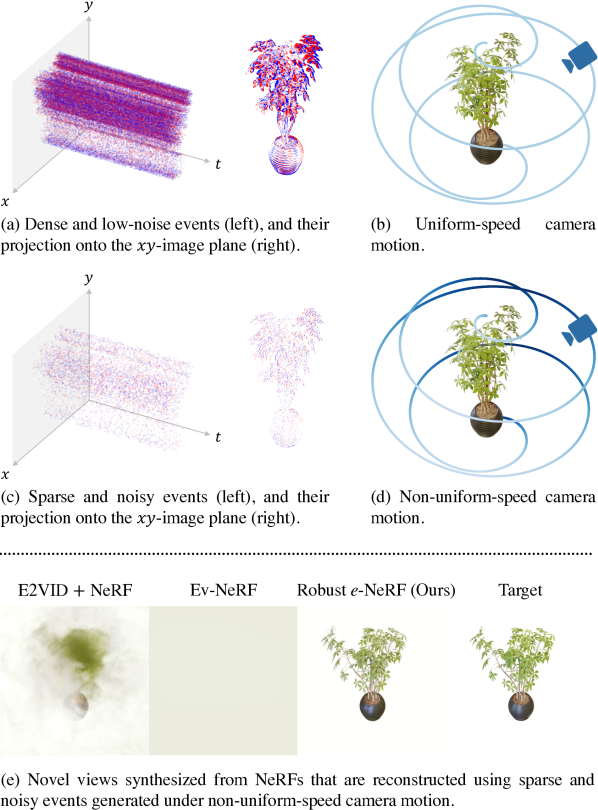
Figure 1: Existing works on NeRF reconstruction from moving event cameras heavily rely on (a) temporally dense and low-noise events generated under roughly (b) uniform-speed camera motion. In contrast, our method, Robust e-NeRF is able to directly and robustly reconstruct NeRFs from (c) sparse and noisy events generated under (d) non-uniform camera motion, as shown in (e).

1 Introduction

Event cameras are bio-inspired sensors that represent a paradigm shift in visual acquisition and processing. This is attributed to its fundamentally distinctive principle of operation, where its pixels independently respond to log-intensity changes in an asynchronous manner, yielding a stream of events, rather than measuring absolute linear intensity synchronously at a constant rate, as done in standard cameras. Such unique properties contribute to their multitude of advantages over standard cameras [9]: low power, low latency, high temporal resolution and high dynamic range, thereby the recent success of event-based [16, 41, 10, 7, 42] or event-image hybrid [53, 52, 12] applications.

The success of many downstream visual applications in robotics, computer vision, graphics and virtual/augmented reality also hinges on an efficient and effective representation to encode various information of the scene being interacted with. Neural scene representations [27, 32, 54, 59, 23], especially neural fields [57], have recently emerged as promising candidates for future applications, owing to their continuous nature and memory efficiency. This trend is further driven by the exceptional capabilities and photo-realism of Neural Radiance Field (NeRF) [27]-based works [54, 26, 50, 34, 35, 36].

Motivated by such promise and potential of event cameras and NeRF, we are interested in studying the following research question: How to robustly reconstruct a NeRF from a moving event camera under general real-world conditions? One simple way is to retrofit an events-to-video reconstruction method [42, 49, 33] to NeRF. However, such a naïve approach is inherently limited by the low photometric accuracy and consistency of the reconstructed video frames, since they are assumed to be true observations of the scene.

On the contrary, recent works, such as EventNeRF [45], Ev-NeRF [13] and E-NeRF [20], have proposed to reconstruct NeRFs directly using events via alternative reconstruction losses inspired or derived from an event generation model. Nonetheless, these works heavily rely on a temporally dense and low-noise event stream, which is generally inaccessible in practice due to the presence of refractory period (i.e. pixel dead-time after generating an event) and pixel-to-pixel variation in the contrast threshold (i.e. minimum log-intensity change for event generation). Such a limitation can be partly attributed to the accumulation of successive events at each pixel over time intervals, as performed in these works. Moreover, the reduction in contrast sensitivity resulting from the event accumulation also leads to a loss of detail in the reconstruction.

In addition, these methods do not directly and effectively generalize to arbitrary contrast threshold values and camera speed profiles, as their optimal hyper-parameter configuration greatly depends on the contrast threshold and speed of motion. EventNeRF and E-NeRF assumes symmetric positive and negative thresholds, which generally does not hold true in practice. While joint optimization of the contrast threshold is supported in Ev-NeRF, an additional regularization is necessary to prevent degeneracy. Furthermore, the assumption of time-varying thresholds made in Ev-NeRF and E-NeRF, which is not well supported by the literature, also leads to a reduction in reconstruction accuracy as shown in our experiments.

Contributions.

We propose Robust e-NeRF, a novel method to directly and robustly reconstruct NeRFs from moving event cameras under various real-world conditions, especially from temporally sparse and noisy event streams given by event cameras in non-uniform motion.

In particular, we incorporate a more realistic event generation model that accounts for various intrinsic parameters (e.g. time-independent, asymmetric contrast threshold and refractory period) and non-idealities (e.g. pixel-to-pixel threshold variation). Furthermore, we introduce two complementary normalized reconstruction losses that are not only effectively invariant to the camera motion speed and threshold scale, but also minimally influenced by asymmetric thresholds. This allows for their effective generalization, as well as the regularization-free joint optimization of unknown contrast threshold and refractory period from poor initializations. The first loss serves as the primary loss for high-fidelity reconstruction, while the second acts as a smoothness constraint for better regularization of textureless regions. As both loss functions do not involve event accumulation, detailed and robust reconstruction from sparse and noisy events can be achieved. Our experiments on novel sequences, simulated using an improved version of ESIM [40], and real sequences from TUM-VIE [19] verify the effectiveness of Robust e-NeRF. We publicly release our code, synthetic event dataset and improved ESIM.

2 Related Work

Event-based Scene Reconstruction.

Successful reconstruction of geometry, and possibly appearance, from events has been demonstrated in notable works, such as [39, 10, 61, 41, 16, 62]. Nonetheless, reconstruction of scene appearance is largely limited to diffuse surfaces due to the adoption of Lambertian surface assumption via brightness constancy [41, 16]. Moreover, existing methods can mainly recover semi-dense geometry, in the form of discrete depth maps or point clouds, corresponding to edges (more precisely, locations with high perceived spatial intensity gradient) in the scene. This is due to the fact that events are primarily generated along edges under relative motion [9].

While [56] achieved dense diffuse reconstruction by applying the classic Structure-from-Motion (SfM) and Multi-View Stereo (MVS) pipelines on video frames reconstructed from events [42], its performance is intrinsically limited by the accuracy of the recovered frames, as similarly discussed in Sec. 1. Although limited to simple, object-level mesh or specialized parametric models, [46, 29, 58] also demonstrated dense diffuse reconstruction via Analysis-by-Synthesis or equivalently Vision-as-Inverse-Graphics [14]. In contrast, we aim to reconstruct dense, continuous scene geometry and view-dependent appearance, in the form of a NeRF, directly from the raw event stream.

Reconstructing Neural Radiance Fields.

In general, visual reconstruction of neural scene representations, including NeRFs, is achieved via Analysis-by-Synthesis. Nonetheless, NeRF derivatives mainly focus on the reconstruction from dense [24, 4, 5] or sparse [30, 17] multi-view images, possibly with depth maps [2, 3] or point clouds [44, 6, 43].

The reconstruction of NeRFs from events was first proposed and investigated in Ev-NeRF [13], E-NeRF [20] and EventNeRF [45]. E-NeRF also explored on using a combination of events and images for NeRF reconstruction. However, these works suffer from various limitations, as outlined in Sec. 1. Moreover, EventNeRF also relies on the access to the analytic camera trajectory, in contrast to E-NeRF and our work which only require constant-rate camera poses. Furthermore, inconsistent sets of loss functions and hyper-parameters were also adopted across different scenes in E-NeRF. In addition, E-NeRF with normalized and no-event losses also requires the contrast threshold to be known as a priori, which is hard to achieve in practice.

3 Our Method

We first briefly introduce the Neural Radiance Field (NeRF) scene representation (Sec. 3.1) . Next, we detail the event generation model (Sec. 3.2) and normalized training losses (Sec. 3.3) proposed to robustly reconstruct NeRFs from event cameras. Lastly, we describe a Gamma Correction-based approach to align the radiance levels of the synthesized views to a set of given reference views (Sec. 3.4).

3.1 Preliminaries: Neural Radiance Fields

Neural Radiance Field (NeRF) [27] represents a scene using a Multi-Layer Perceptron (MLP) $F_{\Theta}:(\bm{x},\bm{d})\mapsto(\bm{c},\sigma)$ that maps 3D position $\bm{x}=(x,y,z)$ and 2D viewing direction $\bm{d}=(\theta,\phi)$ to its corresponding directional emitted radiance, or simply color, $\bm{c}=(r,g,b)$ and volume density $\sigma$. From this representation, the estimated incident radiance $\hat{\bm{L}}$ at a given pixel $\bm{u}$ can be computed using the volume rendering equation with quadrature [51], as follows:

$$\begin{split}\hat{\bm{L}}(\bm{u})&=\sum_{i=1}^{N}T_{i}(1-\exp(-\sigma_{i}\delta_{i}))\bm{c}_{i}\ ,\\ T_{i}&=\exp(-\sum_{j=1}^{i-1}\sigma_{j}\delta_{j})\ ,\end{split}$$ (1)

where $\sigma_{i}$ and $\bm{c}_{i}$ are the volume density and emitted radiance, respectively, of a sample $\bm{x}_{i}$ along the back-projected ray through the pixel, which has direction $\bm{d}$ from the camera center $\bm{o}$. The sample $\bm{x}_{i}=\bm{o}+s_{i}\bm{d}$ has a distance $s_{i}$ from the camera center and a distance of $\delta_{i}=s_{i+1}-s_{i}$ between its adjacent sample $\bm{x}_{i+1}$.

3.2 Event Generation Model

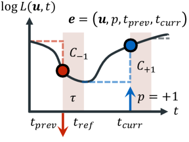
Figure 2: Event generation model. An event $\bm{e}$ of polarity $p$ is generated at timestamp $t_{\mathit{curr}}$ when the difference in log-radiance $\log L$ at a pixel $\bm{u}$, measured with respect to a reference $\log L$ at timestamp $t_{\mathit{ref}}$, has the same sign as $p$ and a magnitude that equals to the contrast threshold associated to polarity $p$, $C_{p}$. Red, downwards and blue, upwards arrows represent events of polarities $-1$ and $+1$, respectively, and each right-angled dashed line represents the measured change in $\log L$. After an event is generated, the pixel will be temporarily deactivated for an amount of time given by the refractory period $\tau$, as shaded in the figure. Thus, $t_{\mathit{ref}}$ is simply the sum of the previous event timestamp $t_{\mathit{prev}}$ and $\tau$.

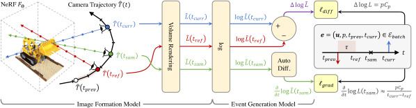
Figure 3: Overview of Robust e-NeRF training. For each event $\bm{e}$ in the batch $\mathcal{E}_{\mathit{batch}}$ sampled randomly from the event stream, we first derive the reference timestamp $t_{\mathit{ref}}$ (Eq. 4), given the refractory period $\tau$, and sample a timestamp $t_{\mathit{sam}}$ between $t_{\mathit{ref}}$ and $t_{\mathit{curr}}$. Next, we interpolate the given constant-rate camera poses at $t_{\mathit{ref}},t_{\mathit{sam}}$ and $t_{\mathit{curr}}$ using LERP for position and SLERP for orientation. Given these pose estimates $\hat{T}$, we then perform volume rendering on the back-projected rays from pixel $\bm{u}$ with the NeRF $F_{\Theta}$ (Eq. 1). This is done to infer the predicted radiance $\hat{L}$, and thus log-radiance $\log{\hat{L}}$, of pixel $\bm{u}$ at $t_{\mathit{ref}},t_{\mathit{sam}}$ and $t_{\mathit{curr}}$. For brevity, we denote $\hat{L}(t)=\hat{L}(\bm{u},t)$. These $\log{\hat{L}}$ are ultimately used to derive the predicted log-radiance difference $\Delta\log\hat{L}$ and gradient $\frac{\partial}{\partial t}\log\hat{L}(t_{\mathit{sam}})$ for the computation of the reconstruction loss: threshold-normalized difference loss $\ell_{\mathit{diff}}$ (Eq. 6) and smoothness loss: target-normalized gradient loss $\ell_{\mathit{grad}}$ (Eq. 7), given the observed log-radiance difference $\Delta\log L$ (Eq. 3) and gradient $\frac{\partial}{\partial t}\log L(t_{\mathit{sam}})$ approximation from the event $\bm{e}$, respectively.

Fig. 2 shows the illustration of the event generation model. An event camera responds to log-radiance changes in the scene and outputs an Event Stream $\mathcal{E}$, given by:

$$\mathcal{E}=\{\ \bm{e}\mid\bm{e}=(\bm{u},p,t_{\mathit{prev}},t_{\mathit{curr}})\ \}\ ,$$ (2)

where $\bm{e}$ is an Event generated by pixel $\bm{u}$, with polarity $p\in\{-1,+1\}$, at timestamp $t_{\mathit{curr}}$. For convenience of discussion, we augment each event with the timestamp of the previous event that was generated by the same pixel, $t_{\mathit{prev}}$.

An event of polarity $p$ is generated when the difference in log-radiance at a pixel, measured with respect to a reference log-radiance at timestamp $t_{\mathit{ref}}$, has the same sign as $p$ and a magnitude that equals to the Contrast Threshold associated to polarity $p$, $C_{p}$ [9]. In short, the condition is given by:

$$\Delta\log L\vcentcolon=\log L(\bm{u},t_{\mathit{curr}})-\log L(\bm{u},t_{\mathit{ref}})=pC_{p}\ ,$$ (3)

where $L$ denotes the incident radiance at the given pixel and timestamp. For color event cameras, $L$ corresponds to the radiance of the incident light after passing through the specific color filter in front of the pixel.

After an event is generated, the pixel will be deactivated for an amount of time specified by the Refractory Period $\tau$. During this period of time, the pixel is invariant to any change in log-radiance and thus will not generate any new events. At the end of the refractory period, the pixel will be reactivated and the current log-radiance value at the pixel will be set as the new reference value, enabling the next event to be generated at this pixel [9, 22]. In essence:

$$t_{\mathit{ref}}=t_{\mathit{prev}}+\tau\ .$$ (4)

The refractory period gives rise to temporal sparsity in the event stream. While this leads to partially observable log-radiance changes, it also limits the event generation rate of the camera [9, 22]. This is crucial to prevent the corruption of event timestamps due to Address Event Representation (AER) bus saturation and readout congestion, especially when the resolution and/or the speed of the camera are high [9, 1, 38, 8]. The bounded event rate also facilitates longer periods of recordings given a fixed memory budget. Furthermore, long refractory periods, as well as asymmetric contrast thresholds, contribute to a lower Shot Noise event rate [25], thereby improving Signal-to-Noise Ratio (SNR).

Event sensors also suffer from non-uniformity of pixel response, similar to standard image sensors. This is characterized by the pixel-to-pixel variation in the contrast threshold, which can be viewed as the event sensor analogue of Fixed-Pattern Noise (FPN). Studies suggest that the threshold variation can be modeled as a Gaussian distribution with mean $C_{p}$ [9, 22, 37].

The contrast threshold is also effectively constant over time, as it is independent of temperature. The key assumption for temperature-independence is the absence of junction leakage [31], which holds true for modern event cameras [48]. Regardless of leakage, temperature-independence remains observed over a large temperature range [31].

3.3 Training

3.3.1 Assumptions

To reconstruct a NeRF from an event camera in motion, we assume that we are given the intrinsic camera matrix, lens distortion parameters and constant-rate camera poses of sufficiently high sampling rate for accurate interpolation at arbitrary time instants. Similar to [20], we perform Linear Interpolation (LERP) on camera positions and Spherical Linear Interpolation (SLERP) on camera orientations. While our method does not rely on event camera-specific intrinsic parameters such as contrast threshold and refractory period to be known as a priori, this information generally facilitates a more accurate reconstruction. As we will see in Sec. 3.3.2, it is also acceptable to provide only the (positive-to-negative) contrast threshold ratio $\nicefrac{{C_{+1}}}{{C_{-1}}}$, which can be inferred from event camera bias settings.

3.3.2 Fundamental Limitations

As event cameras only provide (partial) observations of log-radiance changes, not absolute log-radiance, the predicted log-radiance $\log\hat{\bm{L}}$, given by volume renderings from the reconstructed NeRF (Eq. 1), is only accurate up to an offset per color channel. Furthermore, there will be an additional scale ambiguity that is consistent across all channels, when only the contrast threshold ratio is known. This is similar to an image with unknown black levels and ISO. Nonetheless, these ambiguities can be easily dealt with or corrected for post-reconstruction, e.g. using a set of reference images of the same scene (Sec. 3.4), thereby not a cause for concern. We are also restricted to the reconstruction of a NeRF with single-channel directional emitted radiance, when a monochrome event camera is employed.

3.3.3 Loss Functions

An overview of the training pipeline is illustrated in Fig. 3. In line with the event generation model (Sec. 3.2), we propose two complementary normalized loss functions: threshold-normalized difference loss $\ell_{\mathit{diff}}$ and target-normalized gradient loss $\ell_{\mathit{grad}}$ that directly and effectively generalize to various real-world conditions. The weighted sum of the two losses form the total training loss, which is optimized on a batch of events $\mathcal{E}_{\mathit{batch}}$ sampled randomly from the raw, asynchronous event stream. Formally, the total training loss is given by:

$$\mathcal{L}=\frac{1}{\lvert\mathcal{E}_{\mathit{batch}}\rvert}\sum_{\bm{e}\in\mathcal{E}_{\mathit{batch}}}\lambda_{\mathit{diff}}\ell_{\mathit{diff}}(\bm{e})+\lambda_{\mathit{grad}}\ell_{\mathit{grad}}(\bm{e})\ ,$$ (5)

where $\lambda_{\mathit{diff}}$ and $\lambda_{\mathit{grad}}$ are the respective loss weights.

We specifically refrained from optimizing on a reduced event stream, obtained by accumulating successive events at each pixel over time intervals, as done in [45, 13, 20]. This enables us to account for the refractory period and prevent unnecessary effective reduction in contrast sensitivity, which leads to lower reconstruction fidelity. Moreover, it can also be shown that event accumulation results in the effective amplification of threshold variation (proof in supplementary materials), thereby reduction in noise robustness.

Threshold-Normalized Difference Loss.

This loss enforces the mean contrast threshold $\bar{C}=\frac{1}{2}(C_{-1}+C_{+1})$ normalized squared consistency between the observed log-radiance difference $\Delta\log L=pC_{p}$ from an event (Eq. 3) and the predicted log-radiance difference $\Delta\log\hat{L}\vcentcolon=\log\hat{L}(\bm{u},t_{\mathit{curr}})-\log\hat{L}(\bm{u},t_{\mathit{ref}})$, given by renders from the NeRF model (Eq. 1), as follows:

$$\ell_{\mathit{diff}}(\bm{e})=\left(\frac{\Delta\log\hat{L}-pC_{p}}{\bar{C}}\right)^{2}\ .$$ (6)

Note that when a color event camera is employed, $\hat{L}$ refers to the single-channel rendered radiance, where the color channel is governed by the pixel color filter.

The loss serves as the primary reconstruction loss and can be effectively interpreted as a squared percentage error, especially under symmetric contrast thresholds. The normalization entails that the loss is invariant to the common scale of the positive and negative thresholds, as well as the predicted log-radiance, and only dependent on their ratio. Moreover, the normalization is optimal in the sense that the magnitude of the normalized target $\left\lvert\nicefrac{{pC_{p}}}{{\bar{C}}}\right\rvert=\nicefrac{{C_{p}}}{{\bar{C}}}$ is always centered at 1 regardless of the threshold ratio (proof in supplementary materials). The loss can therefore effectively generalize to arbitrary threshold values.

Unlike Ev-NeRF [13], these properties also enable the joint optimization of the unknown contrast threshold without additional regularization, as it does not suffer from any degeneracy. However, only the contrast threshold ratio can be recovered, thereby an additional scale ambiguity in the predicted log radiance, as mentioned in Sec. 3.3.2. In addition, our experiments also demonstrate the viability of jointly optimizing the refractory period $\tau$ via $t_{\mathit{ref}}$ (Eq. 4).

Target-Normalized Gradient Loss.

This loss is simply the Absolute Percentage Error (APE) of the predicted log-radiance temporal gradient derived using auto-differentiation $\frac{\partial}{\partial t}\log\hat{L}(\bm{u},t)$, with respect to the finite difference approximation of the target log-radiance gradient $\frac{\partial}{\partial t}\log L(\bm{u},t)\approx\frac{pC_{p}}{t_{\mathit{curr}}-t_{\mathit{ref}}}$, at a timestamp $t_{\mathit{sam}}$ sampled between $t_{\mathit{ref}}$ and $t_{\mathit{curr}}$, as follows:

$$\ell_{\mathit{grad}}(\bm{e})=\scalebox{0.95}{$\operatorname{APE}$}\left(\frac{\partial}{\partial t}\log\hat{L}(\bm{u},t_{\mathit{sam}})\genfrac{}{}{0.0pt}{}{}{,}\ \frac{pC_{p}}{t_{\mathit{curr}}-t_{\mathit{ref}}}\right)$$ (7)

where $\operatorname{APE}\left(\hat{y},y\right)=\left\lvert\frac{\hat{y}-y}{y}\right\rvert$. As the finite difference approximation error is minimum at the midpoint and maximum at the endpoints, we sample $t_{\mathit{sam}}$ from a truncated normal distribution that is centered at the midpoint and has a standard deviation of $\nicefrac{{1}}{{4}}$ the interval.

The loss acts as a smoothness constraint for log-radiance changes between $t_{\mathit{ref}}$ and $t_{\mathit{curr}}$, which lack explicit regularization from $\ell_{\mathit{diff}}$. This is particularly important for the effective reconstruction of textureless regions in the scene, where events associated have comparably longer intervals. In contrast to analogous regularization losses adopted in recent works [45, 13, 20], $\ell_{\mathit{grad}}$ is specifically invariant to the speed of motion, hence generalizable to arbitrary speed profiles. An unnormalized gradient loss would over-emphasize events generated under high-speed motion, as they have relatively larger target gradients. Furthermore, the loss is invariant to the common scale of the threshold and predicted log-radiance, similar to $\ell_{\mathit{diff}}$. It is therefore also able to effectively generalize to arbitrary threshold values and facilitate joint optimization of unknown threshold.

3.4 Gamma Correction of Synthesized Views

As alluded in Sec. 3.3.2, the channel-consistent scale and per-channel offset ambiguity in the predicted log-radiance can be corrected for post-reconstruction, given a set of reference images of the same scene. To better account for the likely mismatch of spectral sensitivity, thereby color balance, between the event camera and the standard camera used to capture the reference images. Akin to [45], we further relax the channel-consistent scale to per-channel scales. This entails an affine correction of the predicted log-radiance, or equivalently a gamma correction of the predicted linear radiance, for each color channel as follows:

$$\log\hat{\bm{L}}_{\mathit{corr}}=\bm{a}\odot\log\hat{\bm{L}}+\bm{b}\ ,$$ (8)

where $\bm{a}$ and $\bm{b}$ are the correction parameters, is necessary and sufficient for the reference alignment. Consequently, given the target log-radiance $\log\bm{L}$ from the reference images, the optimal correction parameters can be simply derived via ordinary least squares.

4 Experiments

We adopt Novel View Synthesis (NVS) as the standard task to verify that our method, Robust e-NeRF can indeed directly and robustly reconstruct NeRFs from moving event cameras under various real-world conditions, particularly from sparse and noisy events generated under non-uniform motion. The NVS benchmark experiments are conducted on both synthetic (Sec. 4.1) and real sequences (Sec. 4.2). In addition, we perform ablation studies (Sec. 4.3) to investigate the significance of various components in our method.

Metrics.

We adopt a consistent set of metrics to assess the performance of a method in all experiments. In particular, we employ the three following standard metrics: Peak Signal-to-Noise Ratio (PSNR), Structural Similarity Index Measure (SSIM) [55] and AlexNet-based Learned Perceptual Image Patch Similarity (LPIPS) [60] to quantify the similarity between the gamma-corrected (Sec. 3.4) synthesized novel views and given target novel views.

Baselines.

We benchmark our method, Robust e-NeRF against a recent work, Ev-NeRF [13] and a naïve baseline, E2VID $+$ NeRF, given by cascading the seminal events-to-video reconstruction method, E2VID [42] to NeRF. For Ev-NeRF, events are accumulated over non-overlapping time intervals of $\nicefrac{{1}}{{24}}\ s\approx 41.67\ \mathit{ms}$, as suggested in their paper. To facilitate a fair comparison, all methods, including ours, have been (re-)implemented to adopt a common NeRF backbone. While we do not explicitly compare against E-NeRF [20] and EventNeRF [45], our experiment results should still provide an accurate indication on their performance relative to ours since they share a lot of similarities with Ev-NeRF as detailed in Sec. 1.

Datasets.

The synthetic experiments are performed on a novel set of sequences simulated on the “Realistic Synthetic $360^{\circ}$” scenes, which were adopted in the synthetic experiments of NeRF [27]. These scenes contain a wide variety of photo-realistic objects with complicated structure and non-Lambertian effects, thereby effective for NVS evaluation. The new synthetic event dataset allows for a retrospective comparison between event-based and image-based NeRF reconstruction methods, as the sequences were simulated under highly similar conditions, unlike in [45, 13].

The events are generated from a virtual event camera moving in a hemi-/spherical spiral motion about the object at the origin, as shown in Fig. 1(b, d), using an improved version of ESIM [40], which is an efficient and realistic event simulator. Specifically, we added support to time-independent pixel-to-pixel threshold variation and Blender, circumvented singularities in the trajectory orientation interpolation, as well as improved event simulation accuracy, especially with non-zero refractory periods. On the contrary, the real experiments are performed on the mocap-1d-trans and mocap-desk2 sequences of the TUM-VIE dataset [19], which are mainly forward-facing captures of a desk with various objects on top, under linear and spiral camera motion, respectively. These real sequences were chosen for their relative suitability for NVS and their adoption of a modern, high-resolution event sensor — Prophesee Gen 4.

4.1 Synthetic Experiments

The synthetic experiments form the core of the benchmark, as they allow for realistic controlled experiments under various real-world conditions with absolute ground truth, which are otherwise infeasible using real sequences.

All sequences are simulated with a symmetric contrast threshold of $0.25$ (i.e. $C_{-1}=C_{+1}=0.25$), which is the approximate nominal threshold for event sensors such as the Prophesee Gen 3.1, Gen 4.1 and Sony IMX636 sensor, hence providing a known threshold ratio of 1 (i.e. $\nicefrac{{C_{+1}}}{{C_{-1}}}=1$). The event camera trajectory is also sampled at a high rate of $1\ \mathit{kHz}$ to minimize the influence of pose errors on the performance assessment. Furthermore, the virtual event camera revolves the object 4 times, with uniform 1 revolution per second speed about the object vertical axis by default, similar to [45]. Unless otherwise stated, a sequence is also simulated with zero pixel-to-pixel threshold standard deviation and refractory period (i.e. $\sigma_{C_{p}}=0,\tau=0$). By default, Ev-NeRF and our method are trained with a constant symmetric contrast threshold, given by the prior knowledge of time-independent threshold ratio.

	$v=1\times$				$v_{b}=8\times$				$v=\frac{1}{8}\times$				$v=8\times$
Method	PSNR $\uparrow$	SSIM $\uparrow$	LPIPS $\downarrow$		PSNR $\uparrow$	SSIM $\uparrow$	LPIPS $\downarrow$		PSNR $\uparrow$	SSIM $\uparrow$	LPIPS $\downarrow$		PSNR $\uparrow$	SSIM $\uparrow$	LPIPS $\downarrow$
E2VID $+$ NeRF	18.92	0.832	0.316		18.92	0.832	0.316		18.92	0.832	0.316		18.92	0.832	0.316
Ev-NeRF	27.72	0.935	0.087		26.25	0.926	0.102		19.79	0.792	0.326		20.83	0.862	0.198
[HTML]F3F3F3 Robust e-NeRF	28.19	0.945	0.057		28.19	0.945	0.057		28.19	0.945	0.057		28.19	0.945	0.057

Table 1: Effect of speed profile. $v$ denotes the speed of motion relative to the default hemi-/spherical spiral motion with uniform azimuth speed, whereas $v_{b}$ denotes the oscillation factor of the relative speed of motion (i.e. $v={v_{b}}^{\sin{2\pi ft}},f=1\mathit{Hz}$).

		$\sigma_{C_{p}}=0.00$				$\sigma_{C_{p}}=0.03$				$\sigma_{C_{p}}=0.06$
Method	Opt. $C_{p}$	PSNR $\uparrow$	SSIM $\uparrow$	LPIPS $\downarrow$		PSNR $\uparrow$	SSIM $\uparrow$	LPIPS $\downarrow$		PSNR $\uparrow$	SSIM $\uparrow$	LPIPS $\downarrow$
E2VID $+$ NeRF	$-$	18.92	0.832	0.316		18.68	0.827	0.330		18.03	0.808	0.363
	$\times$	27.72	0.935	0.087		24.42	0.895	0.155		8.07	0.841	0.260
Ev-NeRF	$\checkmark$	27.43	0.911	0.123		23.66	0.826	0.261		15.43	0.708	0.441
[HTML]F3F3F3 [HTML]F3F3F3	$\times$	28.19	0.945	0.057		28.14	0.946	0.058		28.23	0.947	0.057
[HTML]F3F3F3 [HTML]F3F3F3Robust e-NeRF	$\checkmark$	28.17	0.946	0.051		27.91	0.946	0.054		28.19	0.948	0.049

Table 2: Effect of pixel-to-pixel threshold variation $\sigma_{C_{p}}$. “Opt. $C_{p}$” refers to jointly optimizing thresholds $C_{p}$ with NeRF parameters $\Theta$.

			$\tau=0\mathit{ms}$				$\tau=8\mathit{ms}$				$\tau=25\mathit{ms}$
Method	Opt. $C_{p}$	Opt. $\tau$	PSNR $\uparrow$	SSIM $\uparrow$	LPIPS $\downarrow$		PSNR $\uparrow$	SSIM $\uparrow$	LPIPS $\downarrow$		PSNR $\uparrow$	SSIM $\uparrow$	LPIPS $\downarrow$
E2VID $+$ NeRF	$-$	$-$	18.92	0.832	0.316		14.87	0.797	0.427		14.15	0.791	0.467
	$\times$	$-$	27.72	0.935	0.087		13.17	0.707	0.559		12.75	0.759	0.528
Ev-NeRF	$\checkmark$	$-$	27.43	0.911	0.123		13.56	0.716	0.528		13.75	0.717	0.569
[HTML]F3F3F3 [HTML]F3F3F3	$\times$	$\times$	28.19	0.945	0.057		26.30	0.934	0.066		25.51	0.929	0.072
[HTML]F3F3F3 [HTML]F3F3F3Robust e-NeRF	$\times$	$\checkmark$	28.18	0.945	0.052		23.43	0.910	0.090		22.48	0.895	0.105

Table 3: Effect of refractory period $\tau$. “Opt. $\tau$” refers to jointly optimizing refractory period $\tau$ with NeRF parameters $\Theta$.

			$v_{b}=1\times,\sigma_{C_{p}}=0.00,\tau=0\mathit{ms}$				$v_{b}=4\times,\sigma_{C_{p}}=0.03,\tau=8\mathit{ms}$				$v_{b}=8\times,\sigma_{C_{p}}=0.06,\tau=25\mathit{ms}$
Method	Opt. $C_{p}$	Opt. $\tau$	PSNR $\uparrow$	SSIM $\uparrow$	LPIPS $\downarrow$		PSNR $\uparrow$	SSIM $\uparrow$	LPIPS $\downarrow$		PSNR $\uparrow$	SSIM $\uparrow$	LPIPS $\downarrow$
E2VID $+$ NeRF	$-$	$-$	18.92	0.832	0.316		14.98	0.796	0.433		14.07	0.801	0.448
	$\times$	$-$	27.72	0.935	0.087		12.33	0.742	0.521		12.05	0.807	0.425
Ev-NeRF	$\checkmark$	$-$	27.43	0.911	0.123		13.06	0.732	0.539		12.27	0.772	0.539
[HTML]F3F3F3 [HTML]F3F3F3	$\times$	$\times$	28.19	0.945	0.057		24.10	0.913	0.086		23.51	0.900	0.110
[HTML]F3F3F3 [HTML]F3F3F3Robust e-NeRF	$\checkmark$	$\checkmark$	28.19	0.946	0.051		20.42	0.875	0.126		18.83	0.836	0.197

Table 4: Collective effect of speed profile, threshold variation and refractory period.

		$v_{b}=1\times,\sigma_{C_{p}}=0.00,\tau=0\mathit{ms}$				$v_{b}=4\times,\sigma_{C_{p}}=0.03,\tau=8\mathit{ms}$				$v_{b}=8\times,\sigma_{C_{p}}=0.06,\tau=25\mathit{ms}$
$\tau$	$\ell_{\mathit{grad}}$	PSNR $\uparrow$	SSIM $\uparrow$	LPIPS $\downarrow$		PSNR $\uparrow$	SSIM $\uparrow$	LPIPS $\downarrow$		PSNR $\uparrow$	SSIM $\uparrow$	LPIPS $\downarrow$
$\times$	$\checkmark$	28.19	0.945	0.057		12.77	0.799	0.372		12.41	0.798	0.412
$\checkmark$	$\times$	27.96	0.943	0.063		23.15	0.899	0.113		22.21	0.879	0.153
[HTML]F3F3F3 $\checkmark$	$\checkmark$	28.19	0.945	0.057		24.10	0.913	0.086		23.51	0.900	0.110

Table 5: Ablation studies on refractory period $\tau$ modeling and target-normalized gradient loss $\ell_{\mathit{grad}}$.

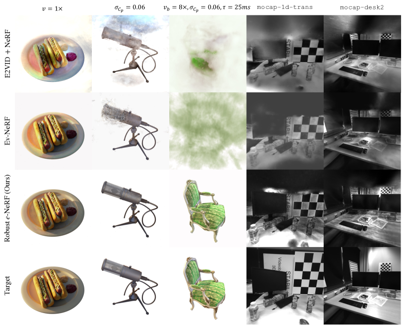
Figure 4: Synthesized novel views in the synthetic and real experiments. Results shown correspond to that with jointly optimized contrast thresholds and possibly refractory period, if applicable for the method in the particular experiment.

Effect of Speed Profile.

To investigate the influence of camera speed, we evaluate all works on 4 sets of sequences simulated with different speed profiles, where each set contains a sequence for each of the 7 scenes. Particularly, the 1^st set is simulated with the default settings, thus providing a reference (uniform azimuth) speed of motion (i.e. $v=1\times$). We oscillate the speed of motion between $\nicefrac{{1}}{{8}}\times$ and $8\times$ the original speed at a frequency of $1\mathit{Hz}$ (i.e. $v={v_{b}}^{\sin{2\pi ft}}$, where $v_{b}=8\times$ and $f=1\mathit{Hz}$) for the 2^nd set, and scale the speed of motion to $\nicefrac{{1}}{{8}}\times$ and $8\times$ of the original speed (i.e. $v=\nicefrac{{1}}{{8}}\times,8\times$) for the 3^rd and 4^th sets, respectively. Fig. 1(b) illustrates the uniform motion in the 1^st, 3^rd and 4^th sets, whereas Fig. 1(d) illustrates the non-uniform, oscillating motion in the 2^nd set.

The quantitative results reported in Tab. 1 underscores the significance of speed invariance in enabling the effective generalization to arbitrary speed profiles, as it can be observed that the performance of Ev-NeRF deteriorates as the speed deviates from the optimal at $v=1\times$. Our method also outperforms all baselines, including Ev-NeRF, at the default setting (i.e. $v=1\times$), which is optimal for all. Qualitative results shown in Fig. 4 suggests an overall improvement in synthesis quality, including high-frequency details.

Effect of Pixel-to-Pixel Threshold Variation.

To evaluate the robustness of our method to noise, in the form of threshold variation, we benchmark all works on three sets of sequences. Furthermore, we also benchmark Ev-NeRF and our method with jointly optimized contrast thresholds, which are poorly initialized with $\nicefrac{{C_{+1}}}{{C_{-1}}}=10$ (more precisely, we set $C_{-1}=0.25$ and $C_{+1}=2.5$), to assess the robustness of the joint optimization. The three sets of sequences were simulated with pixel-to-pixel threshold standard deviations of 0, 0.03 and 0.06 (i.e. $\sigma_{C_{p}}=0.00,0.03,0.06$), which are equivalent to $0\%$, $12\%$ and $24\%$ of the contrast threshold, respectively. $\sigma_{C_{p}}=0.03$ is approximately the nominal value for the Prophesee Gen 3.1, Gen 4 and Sony IMX636 sensor, and $\sigma_{C_{p}}=0.06$ is the maximum value for the Sony IMX636 sensor.

The quantitative results given in Tab. 2 clearly demonstrates the robustness of our method to threshold variation, as our performance is essentially unaffected by the degree of noise. In contrast, the baselines are visibly susceptible to threshold variation, as their performance declines with its severity, especially Ev-NeRF. It is interesting to note that even the naïve baseline outperforms Ev-NeRF at $\sigma_{C_{p}}=0.06$. These conclusions are also supported qualitatively in Fig. 4. The quantitative results also illustrate the effectiveness and robustness of our threshold joint optimization, as the performance of our method with and without jointly optimized thresholds are virtually the same. In contrast, it can be observed that the joint optimization of time-varying contrast thresholds in Ev-NeRF leads to a slight decrease in performance on the default setting (i.e. $\sigma_{C_{p}}=0.00$).

Effect of Refractory Period.

To study the effect of temporal sparsity in the event stream due to the refractory period, we benchmark all methods on three sets of sequences simulated with refractory periods of $0$, $8$ and $25\mathit{ms}$ (i.e. $\tau=0,8,25\mathit{ms}$ ). Similar to the previous experiment, we additionally evaluate our method with jointly optimized refractory period, which is poorly initialized with half the maximum possible value, given by the minimum time interval between successive events at a pixel in the sequence. Furthermore, we also benchmark Ev-NeRF with jointly optimized thresholds to validate the importance of accounting for the refractory period. $\tau=8\mathit{ms}$ is just slightly less than mean event interval in the set of sequences with $\tau=0\mathit{ms}$. Let $\mathcal{E}_{\tau}$ be the event stream with refractory period $\tau$, the degree of sparsity due to $\tau$ can be quantified by the mean $\nicefrac{{\lvert\mathcal{E}_{\tau=0\mathit{ms}}\rvert}}{{\lvert\mathcal{E}_{\tau}\rvert}}$ across all sequences in the set, which translates to $5.84\times$ and $11.37\times$ for $\tau=8$ and $25\mathit{ms}$, respectively.

The quantitative results presented in Tab. 3 undoubtedly verifies the importance of refractory period modeling in enabling the robust reconstruction from temporally sparse event streams, as our method significantly outperforms all baselines across all values of $\tau$. Moreover, the attempt by Ev-NeRF to compensate $\tau$ with jointly optimized thresholds has also clearly failed, albeit contributing to slightly improved performance. It is also worth noting that the naïve baseline achieves better reconstructions than Ev-NeRF under non-zero $\tau$. Our perceivable drop in performance, as $\tau$ increases, may be attributed to its associated decrease in observability. Our results also demonstrate the feasibility of jointly optimizing $\tau$, although less effective than threshold joint optimization, which reflects the complexities involved.

Collective Effect.

To assess the performance of all methods under the collective effect of threshold variation, refractory period and camera speed, which resembles real-world operating conditions, we benchmark all works on three sets of sequences with different levels of difficulty: easy ($\sigma_{C_{p}}=0.00,\tau=0\mathit{ms},v_{b}=1\times$), medium ($\sigma_{C_{p}}=0.03,\tau=8\mathit{ms},v_{b}=4\times$) and hard ($\sigma_{C_{p}}=0.06,\tau=25\mathit{ms},v_{b}=8\times$). In addition, we also benchmark Ev-NeRF and our method with jointly optimized intrinsic parameters, similar to previous experiments. The medium and hard sets are $5.31\times$ and $8.27\times$ sparser than the easy set, respectively. This experiment is particularly challenging as a $K\times$ speed-up effectively scales $\tau$ by $K\times$ in the context of the original sequence. Moreover, methods that involve event accumulation will also experience a $K\times$ effective scaling in $\sigma_{C_{p}}$.

The quantitative results provided in Tab. 4 generally reflect that of the previous experiment, thus the same conclusions can be drawn. This should not be surprising, given the proven importance of accounting for $\tau$. Our decline in performance on the medium and hard settings, when compared to $\tau=8$ and $25\mathit{ms}$, may be attributed to the complications arising from the interaction between $\sigma_{C_{p}}$, $\tau$ and $v_{b}$. Qualitative results given in Fig. 4 illustrates the strength and robustness of our method under challenging conditions.

4.2 Real Experiments

The real experiments mainly serve as a qualitative benchmark, as the dataset (and other similar ones) is not specifically suited for the task of NVS, thereby unable to provide an accurate quantification of performance (refer to supplementary materials for a detailed justification). For the real experiments, Ev-NeRF and our method are trained with jointly optimized intrinsic parameters, where the contrast threshold is initialized with $\nicefrac{{C_{+1}}}{{C_{-1}}}=1$ (more precisely, we set $C_{-1}=C_{+1}=0.25$) this time. While the two sequences mainly involve an insignificant refractory period relative to their primarily non-uniform speed of motion, qualitative results shown in Fig. 4 still demonstrate our superior performance in recovering fine details while appropriately smoothing uniform regions, in line with the synthetic experiments. Exposure of the scene is also visibly more consistent and more accurately reconstructed. Visible artifacts near the borders of all synthesized views are due to the comparably narrower field-of-view of the event camera.

4.3 Ablation Studies

The ablation studies are conducted in the same setting as the synthetic experiment on the collective effect, without jointly optimized intrinsic parameters. The quantitative results reported in Tab. 5 further validates the immense importance of accounting for $\tau$, even when event accumulation is not involved. Although the synthetic sequences mainly involves scenes with abundant texture, the results also verify the effectiveness of the target-normalized gradient loss in regularizing textureless regions, particularly under more challenging conditions (i.e. medium and hard settings).

5 Conclusion

In this paper, we introduce Robust e-NeRF, a novel approach to directly and robustly reconstruct NeRFs from moving event cameras under various real-world conditions, particularly from sparse and noisy events generated under non-uniform motion. Our method consists of two key components: a realistic event generation model that accounts for various event camera-specific intrinsic parameters and non-idealities, as well as a complementary pair of normalized reconstruction losses that can effectively generalize to arbitrary speed profiles and intrinsic parameter values without such prior knowledge. The proposed Analysis-by-Synthesis approach for event-based reconstruction naturally extends to other scene representations, such as 3D Gaussians [15]. In spite of its achievements, Robust e-NeRF still relies on the assumption of a static scene and given constant-rate camera poses, which we leave for future work. We also see the modeling of other spatial/temporal noise and artifacts of an event sensor as a promising future direction for more accurate reconstructions.

Acknowledgements.

This research is supported by the National Research Foundation, Singapore under its AI Singapore Programme (AISG Award No: AISG2-RP-2021-024), and the Tier 2 grant MOE-T2EP20120-0011 from the Singapore Ministry of Education.

Supplementary Material for
Robust e-NeRF: NeRF from Sparse & Noisy Events under Non-Uniform Motion

Weng Fei Low   Gim Hee Lee
The NUS Graduate School’s Integrative Sciences and Engineering Programme (ISEP)
Institute of Data Science (IDS), National University of Singapore
Department of Computer Science, National University of Singapore
{wengfei.low, gimhee.lee}@comp.nus.edu.sg
https://wengflow.github.io/robust-e-nerf

In this supplementary document, we first show how event accumulation results in an effective amplification of pixel-to-pixel contrast threshold variation (Sec. A) and discuss the optimality of normalization in the threshold-normalized difference loss (Sec. B). Next, we present implementation details of Robust e-NeRF and the baselines used in the experiments (Sec. C). We also provide a detailed justification on the qualitative nature of our real experiments (Sec. D). Lastly, we present additional quantitative and qualitative results on all experiments (Sec. E).

Appendix A Amplification of Threshold Variation

As alluded in Sec. 3.3.3, the accumulation of successive events at each pixel over time intervals leads to the effective amplification of pixel-to-pixel contrast threshold variation. This can be shown by simply analyzing the distribution of the target log-radiance difference after event accumulation, at any given pixel.

The time-independent contrast threshold of polarity $p$ can be modeled as a random variable $c_{p}\sim\mathcal{N}(C_{p},{\sigma_{C_{p}}}^{2})$ (Sec. 3.2). Assuming $N_{p}$ number of polarity $p$ events are accumulated at the pixel within the specified time interval, the target log-radiance difference $\Delta\log L_{\mathit{acc}}$ is then given by:

$$\Delta\log L_{\mathit{acc}}=\sum_{p}pN_{p}c_{p}\ ,$$ (9)

which follows the Gaussian distribution below:

$$\mathcal{N}\left(\sum_{p}pN_{p}C_{p},\ \sum_{p}{N_{p}}^{2}{\sigma_{C_{p}}}^{2}-2N_{+1}N_{-1}\sigma_{c_{+1},c_{-1}}\right)\ ,$$ (10)

where $\sigma_{c_{+1},c_{-1}}\in\left[-\sigma_{c_{+1}}\sigma_{c_{-1}},\ \sigma_{c_{+1}}\sigma_{c_{-1}}\right]$ is the covariance between $c_{+1}$ and $c_{-1}$.

Note that when $N_{+1}$ and $N_{-1}$ increases by a factor of $K$, the standard deviation of $\Delta\log L_{\mathit{acc}}$ will also increase by the same factor, which results in noisier targets. Moreover, assuming that $c_{+1}$ and $c_{-1}$ do not have a strong positive correlation (i.e. $\sigma_{c_{+1},c_{-1}}\ll\sigma_{c_{+1}}\sigma_{c_{-1}}$, with respect to the range of $\sigma_{c_{+1}c_{-1}}$), which is highly likely to be true, it can also be shown that standard deviation of $\Delta\log L_{\mathit{acc}}\gg\lvert\sum_{p}pN_{p}\sigma_{C_{p}}\rvert\geq 0$ under non-zero $N_{+1}$ and $N_{-1}$. This suggests that when $N_{+1}C_{+1}\approx N_{-1}C_{-1}$, which often holds true in practice over sufficiently long accumulation intervals (relative to the speed of motion and amount of scene texture), the mean of $\Delta\log L_{\mathit{acc}}=\sum_{p}pN_{p}C_{p}\approx 0$ whereas the standard deviation remains very much larger than 0, especially for large $N_{+1}$ and $N_{-1}$. Such a cancellation between positive and negative accumulated events further aggravates the target noise. All these observations suggest an effective amplification of threshold variation when event accumulation is involved.

Appendix B Optimality of Normalization in $\ell_{\mathit{diff}}$

As mentioned in Sec. 3.3.3, the threshold-normalized difference loss $\ell_{\mathit{diff}}$ (Eq. 6) is optimal in the sense that the magnitude of the normalized target $\left\lvert\nicefrac{{pC_{p}}}{{\bar{C}}}\right\rvert$, which is essentially the normalized threshold $\nicefrac{{C_{p}}}{{\bar{C}}}$, is always centered at 1 regardless of the threshold ratio $\nicefrac{{C_{+1}}}{{C_{-1}}}$, as follows:

$$\left\lvert\frac{pC_{p}}{\bar{C}}\right\rvert=\frac{C_{p}}{\bar{C}}=1+p\frac{\tilde{C}}{\bar{C}}$$ (11)

where $\tilde{C}=\frac{1}{2}(C_{+1}-C_{-1})$ and the magnitude of the offset $\nicefrac{{\tilde{C}}}{{\bar{C}}}$ can be interpreted as the normalized threshold difference. This facilitates the scale consistency of the loss, thus enabling the adoption of a single, global loss weight $\lambda_{\mathit{diff}}$ for arbitrary contrast threshold values. Nevertheless, the variance of the normalized target increases as the thresholds become more asymmetric.

Appendix C Implementation Details

C.1 Robust e-NeRF

Architecture.

Robust e-NeRF adopts Instant-NGP [28] as the NeRF backbone, as it allows for high-quality reconstructions given relatively low training time and memory cost. More precisely, we employ the implementation provided by the NerfAcc toolbox [21], due to its simple and flexible Python APIs, but with some slight modifications.

In particular, parameters of the embedded Multi-Layer Perceptron (MLP) are initialized using the PyTorch-default method, instead of Xavier initialization [11]. Furthermore, we replace all Rectified Linear Unit (ReLU) hidden layer activations with SoftPlus ($\beta=100$) as it is infinitely differentiable everywhere, thereby facilitating the optimization of $\ell_{\mathit{grad}}$.

Since the predicted log-radiance is at most accurate up to an offset per color channel (Sec. 3.3.2), or equivalently the predicted linear radiance (modeled by NeRF) is at most accurate up to a scale per color channel, we also replace the bounded sigmoid radiance output activation with the lower-bounded SoftPlus (default $\beta=1$). In addition, we add a small $\epsilon=0.001$ to the positive raw radiance output from the NeRF model (i.e. $\hat{\bm{L}}=\hat{\bm{L}}_{\mathit{raw}}+\epsilon$) to improve the numerical stability of the predicted log-radiance $\log\hat{\bm{L}}$. This augmentation imposes a lower bound of $\epsilon$ on the radiance our method can model, as $\hat{\bm{L}}>\epsilon$. Nevertheless, this is not a cause for concern given the minimum per-channel scale ambiguity of $\hat{\bm{L}}$, non-upper bounded range of $\hat{\bm{L}}_{\mathit{raw}}$ and non-zero scene radiance (i.e. absolute darkness is virtually impossible in practice).

For synthetic scenes, we also alpha composite $\hat{\bm{L}}_{\mathit{raw}}$ with a learnable background radiance, which is parameterized via SoftPlus to ensure that it is always positive, prior to $\epsilon$-augmentation. In contrast, common NeRF backbones and EventNeRF [45] adopt a fixed background, which is inappropriate given the scale ambiguity.

As only the threshold ratio can be recovered during the joint optimization of contrast threshold (Sec. 3.3.3), we keep the negative threshold $C_{-1}$ fixed at an arbitrary value and only optimize the learnable positive-to-negative contrast threshold ratio $\nicefrac{{C_{+1}}}{{C_{-1}}}$, which is parameterized via SoftPlus to ensure that it is always positive. Moreover, since the refractory period is lower bounded at 0 and upper bounded by the minumum time interval between successive events at any pixel (Sec. 4.1), we parameterize the refractory period via a scaled sigmoid that preserves the gradient profile of the default, unscaled sigmoid function. We additionally clamp the parameterized refractory period between $\varepsilon$ and $(1-\varepsilon)\times$ its range to limit the minimum gradient of the scaled sigmoid to approximately $\varepsilon\times$ the range. This prevents vanishing gradients at the extremes, which implicates the optimization of the refractory period.

For real scenes, we appropriately predefine the Axis-Aligned Bounding Box (AABB), as well as the near and far bounds of the back-projected rays used for volume rendering, for each scene. Furthermore, we employ the spherical space contraction proposed in mip-NeRF 360 [5] to better model unbounded scenes. We also increase the occupancy grid resolution to $256^{3}$ and set the cone angle (i.e. ray marching step size increment scale) to $0.004$, which is approximately $\nicefrac{{1}}{{256}}$ as suggested by Instant-NGP.

Training.

The training loss weights used in all experiments are given by $\lambda_{\mathit{diff}}=1$ and $\lambda_{\mathit{grad}}=0.001$. As suggested by Instant-NGP, we also impose a weight decay of $10^{-6}$ on the MLP to prevent overfitting. The model is trained for 40 000 iterations with a learning rate decay of 0.33 at 20 000, 30 000 and 36 000 iterations (i.e. 50%, 75% and 90% progress, as done in NerfAcc), using the Adam optimizer [18] with a learning rate of 0.01 and PyTorch-default hyper-parameters. During joint optimization of contrast threshold, its parameter is assigned a higher learning rate of 0.1 to facilitate to its early convergence. Moreover, since the scaled sigmoid function preserves its gradient profile, but the range of the refractory period may vary greatly, the learning rate assigned to the (unscaled logit) parameter of refractory period is set to $50\times$ the range. The event batch size is determined dynamically based on the average number of ray samples used to render a single pixel, similar to Instant-NGP, to maximize the utilization of the GPU memory. Specifically, we ensure that every batch of events involves approximately $2^{20}=1\ 048\ 576$ samples in total, for either the rays at $t_{\mathit{ref}}$, $t_{\mathit{curr}}$ (relevant to $\ell_{\mathit{diff}}$) or $t_{\mathit{sam}}$ (relevant to $\ell_{\mathit{grad}}$). As a side note, the poses of the target novel views in the real experiments are interpolated from the given unsynchronized constant-rate camera poses using LERP and SLERP.

C.2 Baselines

As alluded in Sec. 4, both baselines have been carefully reimplemented on the same NerfAcc backbone and trained with the same hyper-parameters (including the weight decay), when applicable, to facilitate a fair comparison. However, we only train the naïve baseline of E2VID $+$ NeRF for 20 000 iterations with a learning rate decay of 0.33 at 10 000, 15 000 and 18 000 iterations (i.e. 50%, 75% and 90% progress) due to its comparably faster convergence, as a result of the direct absolute radiance supervision. Similar to the target novel views, the poses of the E2VID-reconstructed training views are also interpolated from the given unsynchronized constant rate camera poses using LERP and SLERP. Furthermore, we extend the implementation of E2VID to support the RGGB Bayer pattern adopted in ESIM.

Appendix D Justification of Qualitative Real Exps.

As mentioned in Sec. 4.2, we mainly perform qualitative evaluation for the real experiments. This is done because the target novel views, given by a separate standard camera, suffer from saturation due to the comparably smaller dynamic range of the standard camera, and are not raw images that have not been processed by the lossy in-camera image processing pipeline. Moreover, the spectral sensitivity curve of the event camera adopted is also not documented, hence gamma correction may not accurately align the synthesized views.

Furthermore, the comparably narrower field-of-view of the event camera and the limited camera motion also leads to a relatively smaller coverage of the scene, thereby causing artifacts in the synthesized novel views near the borders, as observed in the qualitative results. This further complicates the quantitative evaluation as it is non-trivial to delineate the valid synthesis regions. Other event camera datasets also suffer from similar issues, as all are not specifically suited for novel view synthesis.

Appendix E Additional Experiment Results

E.1 Per-Scene Breakdown

Tab. 6 and Fig. 5, 6 show the quantitative and qualitative results of all methods, respectively, for each of the seven synthetic scene sequences simulated with the default settings, which is optimal for all methods. The per-scene quantitative results is generally consistent with the aggregate metrics, which is also presented in Sec. 4.1, as our method outperforms the baselines in most scenes and has comparable performance in others. The per-scene qualitative results reveal our superior performance in reconstructing fine details and maintaining high color accuracy, especially at the background, as previously observed in Sec. 4.1.

		Synthetic Scene
Metric	Method	chair	drums	ficus	hotdog	lego	materials	mic	Mean
	E2VID $+$ NeRF	19.62	19.52	22.44	17.33	17.41	18.13	18.02	18.92
	Ev-NeRF	28.93	23.89	28.37	25.22	29.10	26.50	32.03	27.72
PSNR $\uparrow$	[HTML]F3F3F3Robust e-NeRF	[HTML]F3F3F330.24	[HTML]F3F3F323.15	[HTML]F3F3F330.71	[HTML]F3F3F328.07	[HTML]F3F3F327.34	[HTML]F3F3F324.98	[HTML]F3F3F332.87	[HTML]F3F3F328.19
	E2VID $+$ NeRF	0.869	0.842	0.863	0.859	0.710	0.835	0.844	0.832
	Ev-NeRF	0.932	0.889	0.948	0.940	0.930	0.926	0.979	0.935
SSIM $\uparrow$	[HTML]F3F3F3Robust e-NeRF	[HTML]F3F3F30.958	[HTML]F3F3F30.897	[HTML]F3F3F30.971	[HTML]F3F3F30.953	[HTML]F3F3F30.934	[HTML]F3F3F30.923	[HTML]F3F3F30.981	[HTML]F3F3F30.945
	E2VID $+$ NeRF	0.277	0.277	0.289	0.341	0.406	0.282	0.337	0.316
	Ev-NeRF	0.085	0.203	0.085	0.103	0.058	0.054	0.024	0.087
LPIPS $\downarrow$	[HTML]F3F3F3Robust e-NeRF	[HTML]F3F3F30.040	[HTML]F3F3F30.091	[HTML]F3F3F30.022	[HTML]F3F3F30.095	[HTML]F3F3F30.074	[HTML]F3F3F30.052	[HTML]F3F3F30.029	[HTML]F3F3F30.057

Table 6: Per-synthetic scene breakdown under the default setting.

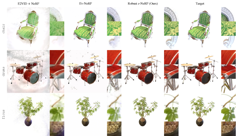
Figure 5: Synthesized novel views on chair, drums and ficus under the default setting.

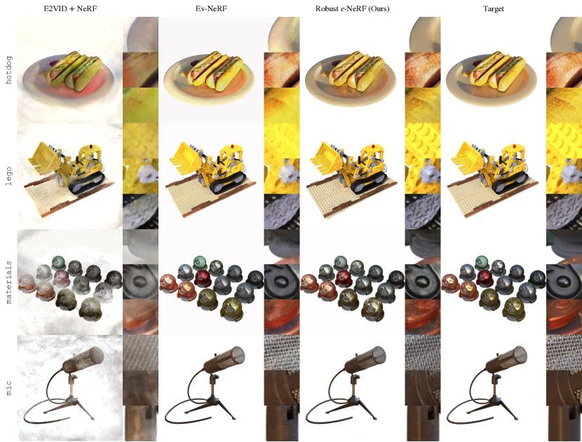
Figure 6: Synthesized novel views on hotdog, lego, materials and mic under the default setting.

E.2 Qualitative Analysis of $\ell_{\mathit{grad}}$

Fig. 7 illustrates the effect of target-normalized gradient loss $\ell_{\mathit{grad}}$ on the hotdog and chair scene sequences simulated with the easy and hard settings, respectively, as similarly done in Sec. 4.3. It can be observed that with $\ell_{\mathit{grad}}$, the plate of the hotdog and the back of the chair exhibit less noise, especially the latter. This is achieved while preserving high-frequency details on the hotdog and the cushion of the chair. This further validates the effectiveness of $\ell_{\mathit{grad}}$ in regularizing textureless regions, particularly under challenging conditions.

E.3 Qualitative Results on office-maze

Apart from mocap-1d-trans and mocap-desk2, we also benchmark all methods on the office-maze sequence from the TUM-VIE dataset. We only employ the subsequence before the 395^th target novel view, as it captures a bounded space of an office (in approximately 2 loops around the office). The qualitative results reported in Fig. 8 clearly shows our effectiveness in recovering details and resolving the scene structure without suffering from severe fogs in free space.

E.4 Robustness to Temporal Event Sparsity

To evaluate the robustness of our method to temporal sparsity of the event stream (i.e. data efficiency), we benchmark it on a set of nine sequences simulated on the synthetic chair scene with different refractory periods. Apart from the standard image similarity performance metrics, we also report some statistics such as the percentage of $\tau$ relative to the duration of the event sequence, as well as the degree of sparsity of the event stream, as defined in Sec. 4.1. Moreover, we also report the number of images that occupy an equivalent amount of memory as the event sequence disregarding compression, assuming 8 bits per image pixel channel and 47 bits per event (i.e. $2\times 11$ bits for position, $1$ bit for polarity and $24$ bits for timestamp), as implied after decompression of the Prophesee EVT 3.0 [47] event encoding format.

The quantitative and qualitative results given in Tab. 7, Fig. 9 and Fig. 10 demonstrate our astonishing robustness under severely sparse event streams, which suggests that our method is highly data efficient. It is worth noting that our method can still reconstruct the scene with reasonable accuracy when $\tau=1000\mathit{ms}$, where only 3 equivalent views are used and each pixel can only generate at most 4 events throughout the $4000\mathit{ms}$ sequence. The event stream is also around $200\times$ sparser than the default with $\tau=0\mathit{ms}$.

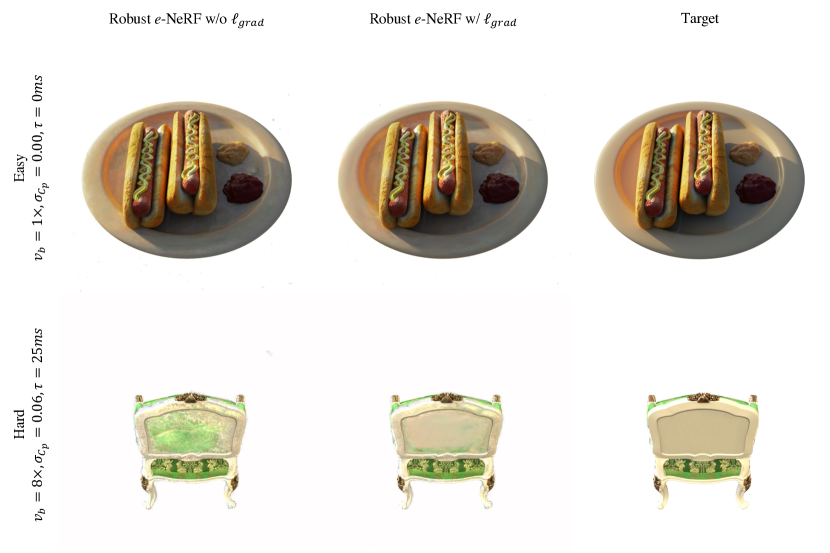
Figure 7: Synthesized novel views with and without the target-normalized gradient loss $\ell_{\mathit{grad}}$.

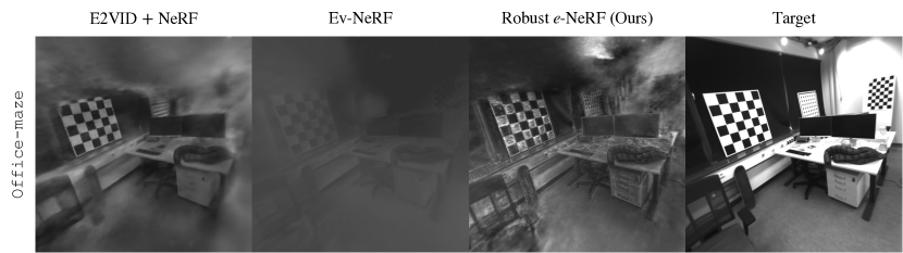
Figure 8: Synthesized novel views on the office-maze scene.

$\tau$, $\mathit{ms}$	Statistics				Metrics
	% Seq. Duration	Sparsity, $\times$	Equiv. # Views		PSNR $\uparrow$	SSIM $\uparrow$	LPIPS $\downarrow$
0	0	1.000	336.8		30.24	0.958	0.040
8	0.2	4.176	80.66		30.41	0.959	0.042
25	0.625	8.440	39.90		29.84	0.958	0.041
50	1.25	13.50	24.95		29.20	0.953	0.046
100	2.5	21.27	15.83		27.40	0.938	0.060
250	6.25	40.80	8.255		25.95	0.916	0.081
500	12.5	67.77	4.970		24.08	0.900	0.102
1000	25	110.5	3.048		22.10	0.854	0.204
2000	50	209.6	1.607		17.05	0.762	0.398

Table 7: Robustness of our method to temporal event sparsity on the chair scene.

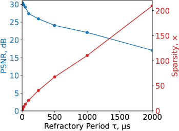
Figure 9: Plot of novel view synthesis PSNR and degree of event sparsity on the chair scene against refractory period $\tau$.

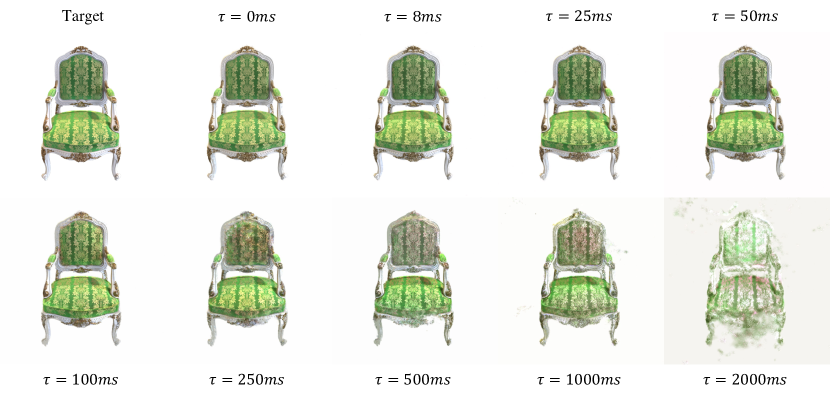
Figure 10: Synthesized novel views on the chair scene under numerous refractory periods $\tau$.

References

- [1] Understanding the performance of neuromorphic event-based vision sensors. Technical report, iniVation AG, 2020.
- [2] Benjamin Attal, Eliot Laidlaw, Aaron Gokaslan, Changil Kim, Christian Richardt, James Tompkin, and Matthew O’Toole. TöRF: Time-of-Flight Radiance Fields for Dynamic Scene View Synthesis. In Advances in Neural Information Processing Systems, 2021.
- [3] Dejan Azinović, Ricardo Martin-Brualla, Dan B Goldman, Matthias Nießner, and Justus Thies. Neural RGB-D Surface Reconstruction. In Proceedings of the IEEE/CVF Conference on Computer Vision and Pattern Recognition (CVPR), 2022.
- [4] J T Barron, B Mildenhall, M Tancik, P Hedman, R Martin-Brualla, and P P Srinivasan. Mip-NeRF: A Multiscale Representation for Anti-Aliasing Neural Radiance Fields. In 2021 IEEE/CVF International Conference on Computer Vision (ICCV), 2021.
- [5] Jonathan T. Barron, Ben Mildenhall, Dor Verbin, Pratul P. Srinivasan, and Peter Hedman. Mip-NeRF 360: Unbounded Anti-Aliased Neural Radiance Fields. In 2022 IEEE/CVF Conference on Computer Vision and Pattern Recognition (CVPR), 2022.
- [6] Kangle Deng, Andrew Liu, Jun-Yan Zhu, and Deva Ramanan. Depth-supervised {NeRF}: Fewer Views and Faster Training for Free. In Proceedings of the IEEE/CVF Conference on Computer Vision and Pattern Recognition (CVPR), June 2022.
- [7] Davide Falanga, Kevin Kleber, and Davide Scaramuzza. Dynamic obstacle avoidance for quadrotors with event cameras. Science Robotics, 2020.
- [8] Thomas Finateu, Atsumi Niwa, Daniel Matolin, Koya Tsuchimoto, Andrea Mascheroni, Etienne Reynaud, Pooria Mostafalu, Frederick Brady, Ludovic Chotard, Florian LeGoff, Hirotsugu Takahashi, Hayato Wakabayashi, Yusuke Oike, and Christoph Posch. 5.10 A 1280720 Back-Illuminated Stacked Temporal Contrast Event-Based Vision Sensor with 4.86m Pixels, 1.066GEPS Readout, Programmable Event-Rate Controller and Compressive Data-Formatting Pipeline. In 2020 IEEE International Solid- State Circuits Conference - (ISSCC), 2020.
- [9] Guillermo Gallego, Tobi Delbrück, Garrick Orchard, Chiara Bartolozzi, Brian Taba, Andrea Censi, Stefan Leutenegger, Andrew J. Davison, Jörg Conradt, Kostas Daniilidis, and Davide Scaramuzza. Event-based vision: A survey. IEEE Transactions on Pattern Analysis and Machine Intelligence, 2020.
- [10] Guillermo Gallego, Henri Rebecq, and Davide Scaramuzza. A Unifying Contrast Maximization Framework for Event Cameras, with Applications to Motion, Depth, and Optical Flow Estimation. In 2018 IEEE/CVF Conference on Computer Vision and Pattern Recognition, 2018.
- [11] Xavier Glorot and Yoshua Bengio. Understanding the difficulty of training deep feedforward neural networks. In Proceedings of the Thirteenth International Conference on Artificial Intelligence and Statistics, 2010.
- [12] Javier Hidalgo-Carrió, Guillermo Gallego, and Davide Scaramuzza. Event-Aided Direct Sparse Odometry. In Proceedings of the IEEE/CVF Conference on Computer Vision and Pattern Recognition (CVPR), 2022.
- [13] Inwoo Hwang, Junho Kim, and Young Min Kim. Ev-nerf: Event based neural radiance field. In 2023 IEEE/CVF Winter Conference on Applications of Computer Vision (WACV), 2023.
- [14] Hiroharu Kato, Deniz Beker, Mihai Morariu, Takahiro Ando, Toru Matsuoka, Wadim Kehl, and Adrien Gaidon. Differentiable Rendering: A Survey, 2020. arXiv:2006.12057 [cs].
- [15] Bernhard Kerbl, Georgios Kopanas, Thomas Leimkuehler, and George Drettakis. 3D Gaussian Splatting for Real-Time Radiance Field Rendering. ACM Trans. Graph., 2023.
- [16] Hanme Kim, Stefan Leutenegger, and Andrew Davison. Real-time 3d reconstruction and 6-dof tracking with an event camera. In Computer Vision - ECCV 2016 - 14th European Conference, Amsterdam, The Netherlands, October 11-14, 2016, Proceedings, Part VI, 2016.
- [17] Mijeong Kim, Seonguk Seo, and Bohyung Han. InfoNeRF: Ray Entropy Minimization for Few-Shot Neural Volume Rendering. In Proceedings of the IEEE/CVF Conference on Computer Vision and Pattern Recognition (CVPR), 2022.
- [18] Diederik P. Kingma and Jimmy Ba. Adam: A method for stochastic optimization. In 3rd International Conference on Learning Representations, ICLR 2015, San Diego, CA, USA, May 7-9, 2015, Conference Track Proceedings, 2015.
- [19] Simon Klenk, Jason Chui, Nikolaus Demmel, and Daniel Cremers. Tum-vie: The tum stereo visual-inertial event dataset. In 2021 IEEE/RSJ International Conference on Intelligent Robots and Systems (IROS), 2021.
- [20] Simon Klenk, Lukas Koestler, Davide Scaramuzza, and Daniel Cremers. E-nerf: Neural radiance fields from a moving event camera. IEEE Robotics and Automation Letters, 2023.
- [21] Ruilong Li, Matthew Tancik, and Angjoo Kanazawa. NerfAcc: A General NeRF Acceleration Toolbox, 2022. arXiv:2210.04847 [cs].
- [22] Patrick Lichtsteiner, Christoph Posch, and Tobi Delbruck. A 128 128 120 dB 15 s latency asynchronous temporal contrast vision sensor. IEEE Journal of Solid-State Circuits, 2008.
- [23] Weng Fei Low and Gim Hee Lee. Minimal Neural Atlas: Parameterizing Complex Surfaces with Minimal Charts and Distortion. In European Conference on Computer Vision (ECCV), 2022.
- [24] Ricardo Martin-Brualla, Noha Radwan, Mehdi SM Sajjadi, Jonathan T Barron, Alexey Dosovitskiy, and Daniel Duckworth. Nerf in the wild: Neural radiance fields for unconstrained photo collections. In Proceedings of the IEEE/CVF Conference on Computer Vision and Pattern Recognition, 2021.
- [25] Brian McReynolds, Rui Graca, and Tobi Delbruck. Exploiting Alternating DVS Shot Noise Event Pair Statistics to Reduce Background Activity. In 2023 International Image Sensor Workshop (IISW), 2023.
- [26] Ben Mildenhall, Peter Hedman, Ricardo Martin-Brualla, Pratul P. Srinivasan, and Jonathan T. Barron. NeRF in the Dark: High Dynamic Range View Synthesis From Noisy Raw Images. In Proceedings of the IEEE/CVF Conference on Computer Vision and Pattern Recognition (CVPR), 2022.
- [27] Ben Mildenhall, Pratul P. Srinivasan, Matthew Tancik, Jonathan T. Barron, Ravi Ramamoorthi, and Ren Ng. NeRF: Representing Scenes as Neural Radiance Fields for View Synthesis. In European Conference on Computer Vision (ECCV) 2020, 2020.
- [28] Thomas Müller, Alex Evans, Christoph Schied, and Alexander Keller. Instant Neural Graphics Primitives with a Multiresolution Hash Encoding. ACM Transactions on Graphics, 2022.
- [29] Jalees Nehvi, Vladislav Golyanik, Franziska Mueller, Hans-Peter Seidel, Mohamed Elgharib, and Christian Theobalt. Differentiable event stream simulator for non-rigid 3d tracking. In Proceedings of the IEEE/CVF Conference on Computer Vision and Pattern Recognition, 2021.
- [30] Michael Niemeyer, Jonathan T Barron, Ben Mildenhall, Mehdi S M Sajjadi, Andreas Geiger, and Noha Radwan. RegNeRF: Regularizing Neural Radiance Fields for View Synthesis from Sparse Inputs. In Proceedings of the IEEE/CVF Conference on Computer Vision and Pattern Recognition (CVPR), 2022.
- [31] Yuji Nozaki and Tobi Delbruck. Temperature and Parasitic Photocurrent Effects in Dynamic Vision Sensors. IEEE Transactions on Electron Devices, 2017.
- [32] Michael Oechsle, Songyou Peng, and Andreas Geiger. Unisurf: Unifying neural implicit surfaces and radiance fields for multi-view reconstruction, 2021.
- [33] F. Paredes-Valles and G. E. de Croon. Back to event basics: Self-supervised learning of image reconstruction for event cameras via photometric constancy. In 2021 IEEE/CVF Conference on Computer Vision and Pattern Recognition (CVPR), 2021.
- [34] Keunhong Park, Utkarsh Sinha, Peter Hedman, Jonathan T Barron, Sofien Bouaziz, Dan B Goldman, Ricardo Martin-Brualla, and Steven M Seitz. HyperNeRF: A Higher-Dimensional Representation for Topologically Varying Neural Radiance Fields. ACM Trans. Graph., 2021.
- [35] Sida Peng, Junting Dong, Qianqian Wang, Shangzhan Zhang, Qing Shuai, Xiaowei Zhou, and Hujun Bao. Animatable neural radiance fields for modeling dynamic human bodies. In Proceedings of the IEEE/CVF International Conference on Computer Vision, 2021.
- [36] Ben Poole, Ajay Jain, Jonathan T. Barron, and Ben Mildenhall. Dreamfusion: Text-to-3d using 2d diffusion. In The Eleventh International Conference on Learning Representations, 2023.
- [37] Christoph Posch and Daniel Matolin. Sensitivity and uniformity of a 0.18m CMOS temporal contrast pixel array. In 2011 IEEE International Symposium of Circuits and Systems (ISCAS), 2011.
- [38] Christoph Posch, Teresa Serrano-Gotarredona, Bernabe Linares-Barranco, and Tobi Delbruck. Retinomorphic Event-Based Vision Sensors: Bioinspired Cameras With Spiking Output. Proceedings of the IEEE, 2014.
- [39] Henri Rebecq, Guillermo Gallego, Elias Mueggler, and Davide Scaramuzza. EMVS: Event-Based Multi-View Stereo—3D Reconstruction with an Event Camera in Real-Time. International Journal of Computer Vision, 2018.
- [40] Henri Rebecq, Daniel Gehrig, and Davide Scaramuzza. ESIM: an Open Event Camera Simulator. In Proceedings of The 2nd Conference on Robot Learning, PMLR, 2018.
- [41] Henri Rebecq, Timo Horstschafer, Guillermo Gallego, and Davide Scaramuzza. Evo: A geometric approach to event-based 6-dof parallel tracking and mapping in real-time. IEEE Robotics and Automation Letters, 2016.
- [42] Henri Rebecq, René Ranftl, Vladlen Koltun, and Davide Scaramuzza. High speed and high dynamic range video with an event camera. IEEE Transactions on Pattern Analysis and Machine Intelligence, 2021.
- [43] Konstantinos Rematas, Andrew Liu, Pratul P Srinivasan, Jonathan T Barron, Andrea Tagliasacchi, Tom Funkhouser, and Vittorio Ferrari. Urban Radiance Fields. In Proceedings of the IEEE/CVF Conference on Computer Vision and Pattern Recognition (CVPR), 2022.
- [44] Barbara Roessle, Jonathan T Barron, Ben Mildenhall, Pratul P Srinivasan, and Matthias Nießner. Dense Depth Priors for Neural Radiance Fields from Sparse Input Views. In Proceedings of the IEEE/CVF Conference on Computer Vision and Pattern Recognition (CVPR), 2022.
- [45] Viktor Rudnev, Mohamed Elgharib, Christian Theobalt, and Vladislav Golyanik. Eventnerf: Neural radiance fields from a single colour event camera, 2022. arXiv:2206.11896 [cs].
- [46] Viktor Rudnev, Vladislav Golyanik, Jiayi Wang, Hans-Peter Seidel, Franziska Mueller, Mohamed Elgharib, and Christian Theobalt. Eventhands: Real-time neural 3d hand pose estimation from an event stream. In Proceedings of the IEEE/CVF International Conference on Computer Vision (ICCV), 2021.
- [47] Prophesee S.A. Evt 3.0 format. https://docs.prophesee.ai/stable/data/encoding_formats/evt3.html.
- [48] Bongki Son, Yunjae Suh, Sungho Kim, Heejae Jung, Jun-Seok Kim, Changwoo Shin, Keunju Park, Kyoobin Lee, Jinman Park, Jooyeon Woo, Yohan Roh, Hyunku Lee, Yibing Wang, Ilia Ovsiannikov, and Hyunsurk Ryu. 4.1 A 640480 dynamic vision sensor with a 9m pixel and 300Meps address-event representation. In 2017 IEEE International Solid-State Circuits Conference (ISSCC), 2017.
- [49] Timo Stoffregen, Cedric Scheerlinck, Davide Scaramuzza, Tom Drummond, Nick Barnes, Lindsay Kleeman, and Robert Mahony. Reducing the Sim-to-Real Gap for Event Cameras. In Computer Vision – ECCV 2020, 2020.
- [50] Edgar Sucar, Shikun Liu, Joseph Ortiz, and Andrew J Davison. imap: Implicit mapping and positioning in real-time. In Proceedings of the IEEE/CVF International Conference on Computer Vision, 2021.
- [51] Andrea Tagliasacchi and Ben Mildenhall. Volume Rendering Digest (for NeRF), 2022. arXiv:2209.02417 [cs].
- [52] Stepan Tulyakov, Daniel Gehrig, Stamatios Georgoulis, Julius Erbach, Mathias Gehrig, Yuanyou Li, and Davide Scaramuzza. Time lens: Event-based video frame interpolation. In 2021 IEEE/CVF Conference on Computer Vision and Pattern Recognition (CVPR), 2021.
- [53] Antoni Rosinol Vidal, Henri Rebecq, Timo Horstschaefer, and Davide Scaramuzza. Ultimate slam? combining events, images, and imu for robust visual slam in hdr and high-speed scenarios. IEEE Robotics and Automation Letters, 2018.
- [54] Peng Wang, Lingjie Liu, Yuan Liu, Christian Theobalt, Taku Komura, and Wenping Wang. Neus: Learning neural implicit surfaces by volume rendering for multi-view reconstruction. In Advances in Neural Information Processing Systems, 2021.
- [55] Zhou Wang, A.C. Bovik, H.R. Sheikh, and E.P. Simoncelli. Image quality assessment: from error visibility to structural similarity. IEEE Transactions on Image Processing, 2004.
- [56] Kun Xiao, Guohui Wang, Yi Chen, Jinghong Nan, and Yongfeng Xie. Event-based dense reconstruction pipeline. In 2022 6th International Conference on Robotics and Automation Sciences (ICRAS), 2022.
- [57] Yiheng Xie, Towaki Takikawa, Shunsuke Saito, Or Litany, Shiqin Yan, Numair Khan, Federico Tombari, James Tompkin, Vincent Sitzmann, and Srinath Sridhar. Neural Fields in Visual Computing and Beyond. Computer Graphics Forum, 2022.
- [58] Yuxuan Xue, Haolong Li, Stefan Leutenegger, and Joerg Stueckler. Event-based non-rigid reconstruction from contours. In 33rd British Machine Vision Conference 2022, BMVC 2022, London, UK, November 21-24, 2022, 2022.
- [59] Lior Yariv, Jiatao Gu, Yoni Kasten, and Yaron Lipman. Volume rendering of neural implicit surfaces. In Advances in Neural Information Processing Systems, 2021.
- [60] R. Zhang, P. Isola, A. A. Efros, E. Shechtman, and O. Wang. The unreasonable effectiveness of deep features as a perceptual metric. In 2018 IEEE/CVF Conference on Computer Vision and Pattern Recognition (CVPR), 2018.
- [61] Yi Zhou, Guillermo Gallego, Henri Rebecq, Laurent Kneip, Hongdong Li, and Davide Scaramuzza. Semi-dense 3d reconstruction with a stereo event camera. In Computer Vision – ECCV 2018: 15th European Conference, Munich, Germany, September 8-14, 2018, Proceedings, Part I, 2018.
- [62] Yi Zhou, Guillermo Gallego, and Shaojie Shen. Event-based stereo visual odometry. IEEE Transactions on Robotics, 2021.