Phase field method for quasi-static hydro-fracture in porous media under stress boundary condition considering the effect of initial stress field

Abstract

Phase field model (PFM) is an efficient fracture modeling method and has high potential for hydraulic fracturing (HF). However, the current PFMs in HF do not consider well the effect of in-situ stress field and the numerical examples of porous media with stress boundary conditions were rarely presented. The main reason is that if the remote stress is applied on the boundaries of the calculation domain, there will be relatively large deformation induced on these stress boundaries, which is not consistent with the engineering observations. To eliminate this limitation, this paper proposes a new phase field method to describe quasi-static hydraulic fracture propagation in porous media subjected to stress boundary conditions, and the new method is more in line with engineering practice. A new energy functional, which considers the effect of initial in-situ stress field, is established and then it is used to achieve the governing equations for the displacement and phase fields through the variational approach. Biot poroelasticity theory is used to couple the fluid pressure field and the displacement field while the phase field is used for determining the fluid properties from the intact domain to the fully broken domain. In addition, we present several 2D and 3D examples to show the effects of in-situ stress on hydraulic fracture propagation. The numerical examples indicate that under stress boundary condition our approach obtains correct displacement distribution and it is capable of capturing complex hydraulic fracture growth patterns.

1 Department of Geotechnical Engineering, College of Civil Engineering, Tongji University, Shanghai 200092, P.R. China
2 Institute of Continuum Mechanics, Leibniz University Hannover, Hannover 30167, Germany
3 Institute of Structural Mechanics, Bauhaus University Weimar, Weimar 99423, Germany
$*$ Corresponding author: Xiaoying Zhuang (zhuang@ikm.uni-hannover.de)

Keywords: Phase field model, Hydraulic fracture, Porous media, Stress boundary, In-situ stress, Staggered scheme

1 Introduction

Hydraulic fracture propagation in porous media is one of the most attractive and significant research topics in mechanical, geological, energy, and environmental engineering. In particular, hydraulic fracturing (HF) [1] has been widely used to exploit oil, tight gas, and shale gas from reservoirs that were unexploitable in past decades. The main reason for this is that the injection of highly pressurized fluid into a reservoir forms a fracture network for resource transportation. Another application of HF is the measurement of in-situ stress [2]. In addition, HF can be also applied in an enhanced geothermal system to accelerate heat extraction [3]. Nevertheless, despite its advantages, HF still brings some controversies because the fracturing fluid may leak and further contaminate the underground space and surface due to unfavorable fracture growth paths [4; 5]. Therefore, an accurate numerical tool is critically important in the prediction of complex hydraulic fracture propagation in porous media.

However, correctly modeling hydraulic fracture in porous media is challenging and full of complexity due to solid-fluid interaction, fracture network, and different boundary conditions. This has prompted the development of various numerical methods for modeling fracturing processes, and these approaches can be classified into two types in the continuum framework: the discrete method and the smeared method. The discrete methods introduce displacement discontinuity for fractures and among the most popular are the extended finite element method (XFEM) [6; 7], generalized finite element method (GFEM) [8], boundary element method [9; 10; 11], phantom-node method [12; 13], and element-erosion method [14; 15]. On the other hand, in the smeared methods the displacement is continuous across a fracture and the gradient damage model [16], the screened Poisson method [17], and the phase field model (PFM) [18; 19; 20; 21; 22] are the best-known.

Among all the fracture modeling methods, the PFMs are attracting more and more attention in recent years. In this method, an additional scalar field $\phi\in[0,1]$ is used to reflect the extent of fracture where $\phi=0$ represents an intact material and $\phi=1$ indicates a fully broken material (some literatures [23] use a phase field $s=1-\phi$ and $s=0$, 1 represents the fully broken state and intact state, respectively). In addition, the transition zone with $\phi\in(0,1)$ is controlled by an intrinsic length scale parameter $l_{0}$. After being first proposed by Bourdin et al. [18], the PFM was further promoted by Bourdin et al. [18]; Miehe et al. [19, 20]; Borden et al. [24]; Hofacker and Miehe [25, 26]. Compared with XIGA [27], XFEM [28; 29], cohesive zone model[30; 31], and continuum damage model [32], PFM has ease of implementation. Furthermore, the recent development has shown that PFMs have a high efficiency in predicting complex fracture propagation patterns, even in 3D situations due to these reasons: i) simulations can be performed on a fixed mesh without any remeshing or adaptive technique; ii) complex fracture patterns such as branching and junction are automatically captured; iii) external fracture criteria or fracture surface tracking algorithms are not required; iv) PFMs can easily simulate fracture propagation in heterogeneous media, and v) no penetration criteria are required for hydraulic fracture when a layer interface is encountered.

The aforementioned advantages have also contributed to the development of PFMs in hydraulic fracturing. For example, in recent years many researchers have tried to couple the PFMs to HF and made some progress [33; 34; 35; 36; 37; 38; 39; 40; 41; 42; 43; 44; 45]. However, the presented examples in these contributions all only established homogeneous Dirichlet boundary conditions for the displacement field. The current PFMs in HF therefore cannot consider well the effect of in-situ stress on fracture propagation. The main reason is that if the remote stress is applied on the boundaries of the calculation domain, there will be relatively large deformation induced on these stress boundaries, which is not consistent with the engineering observations. In fact, in geological environment, the displacement on the boundaries where the remote stress acts should be zero before HF. It should be noted that although a recently developed PFM [46] attempted to analyze the effect of stress boundary condition on fracture pattern, the main drawback remained unsolved because a large deformation was observed on the stress boundaries.

To eliminate the limitation from the initial stress field, this paper proposes a new phase field method to describe quasi-static hydraulic fracture propagation in porous media subjected to stress boundary conditions. A new energy functional, which fully considers the effect of initial in-situ stress field, is established and then it is used to achieve the governing equations of strong form for the displacement and phase fields through the variational approach. Biot poroelasticity theory is used to couple the fluid pressure field and the displacement field while the phase field is used for determining the fluid properties from the intact domain to the fully broken domain. In addition, several 2D and 3D examples are presented to show the effects of in-situ stress on hydraulic fracture propagation. The numerical examples indicate that under stress boundary conditions the new PFM obtains correct displacement distribution and it is capable of capturing well complex hydraulic fracture growth patterns.

This paper is organized as follows. Section 2 describes the mathematical model for the new PFM and Section 3 shows the global numerical algorithm using a staggered scheme. In Sections 4 and 5 the 2D and 3D examples are presented to demonstrate the capability of the new model. The present work and outlook for future development are concluded in Section 6.

2 Mathematical model

2.1 New energy functional

Let us consider a poro-elastic domain $\Omega\subset\mathbb{R}^{d}$ ($d\in\{2,3\}$) in Fig. 1 where the external and internal discontinuity boundaries are denoted as $\partial\Omega$ and $\Gamma$, respectively. The porous medium is assumed homogeneous and isotropic with compressible and viscous fluid in the pores. Let $T>0$ be the computational time interval and $\bm{u}(\bm{x},t)\subset\mathbb{R}^{d}$ be the displacement field at time $t\in[0,T]$ and the position $\bm{x}$. In addition, the displacement field must satisfy the time-dependent Dirichlet boundary conditions, $u_{i}(\bm{x},t)=g_{i}(\bm{x},t)$, on $\partial\Omega_{g_{i}}\in\partial\Omega$, and the Neumann condition on $\partial\Omega_{h}$.

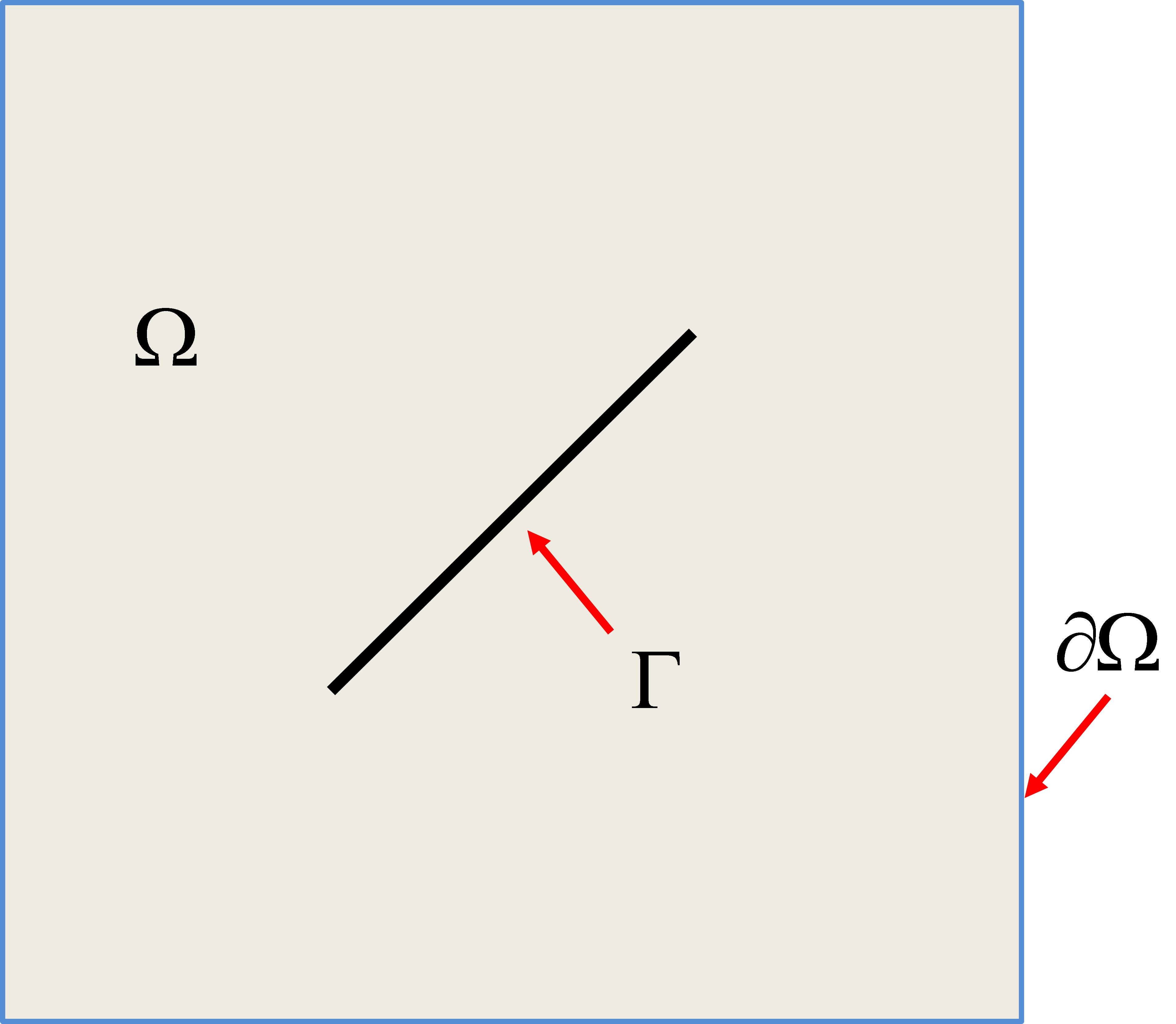
(a) Sharp fracture

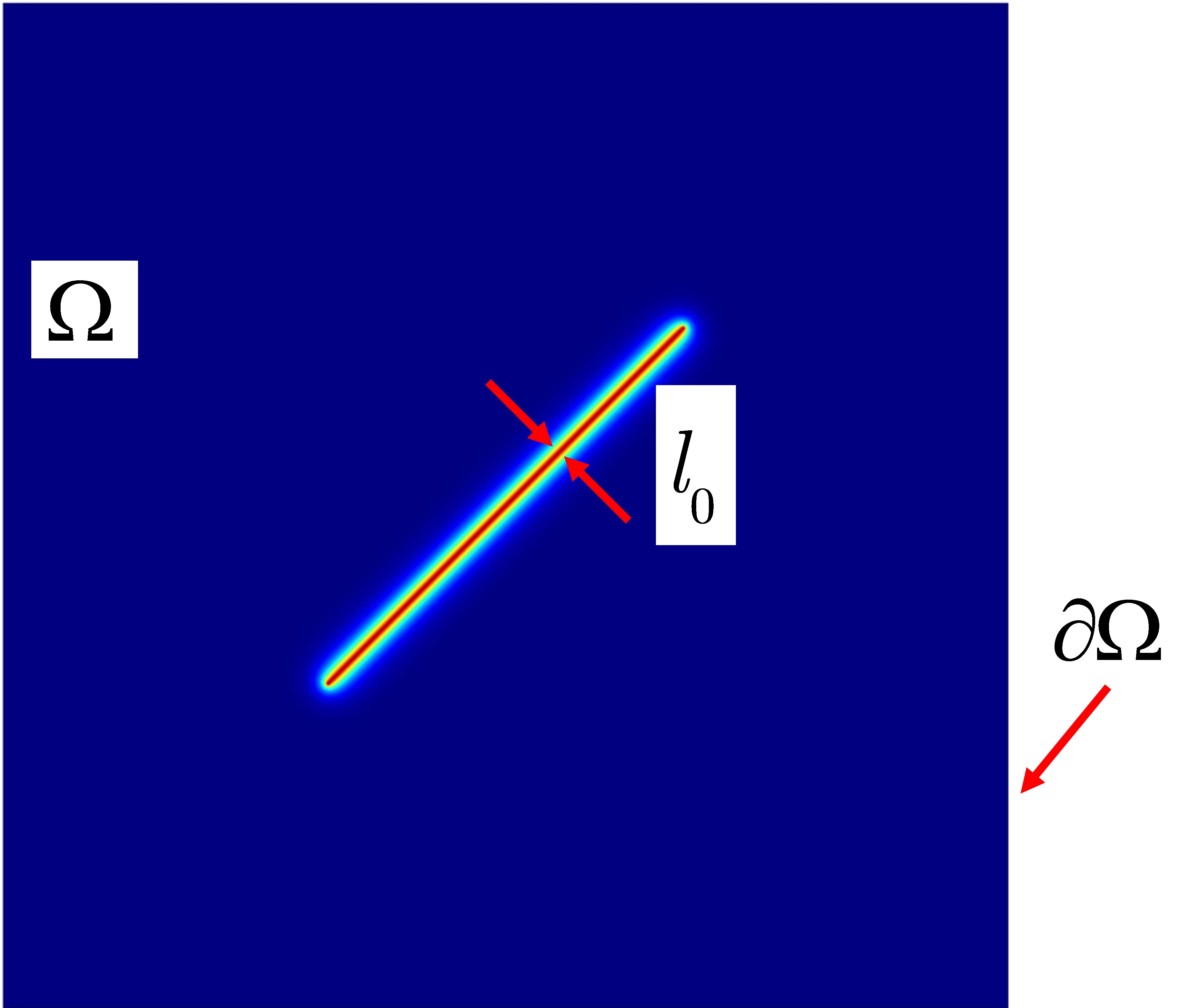
(b) Diffusive fracture

Figure 1: Sharp and diffusive fractures in the poro-elastic medium

The stress, displacement, and fluid pressure of the porous domain are shown in Fig. 2. Because of the long-term consolidation or other geological effects, the domain has formed an initial stress field $\bm{\sigma}_{0}$, initial displacement field $\bm{u}_{0}$, and fluid pressure $p_{0}$, as shown in Fig. 2a. On the other hand, in Fig. 2b, after the domain is excavated or fractured by fluid injection, the stress, displacement, and fluid pressure are $\bm{\sigma}$, $\bm{u}_{0}+\bm{u}$, and $p_{0}+p$, respectively. Here, the displacement $\bm{u}$ and pressure $p$ are the induced relative displacement and fluid pressure by engineering activities such as HF. In this work, our presented method is only for calculating $\bm{\sigma}$, $\bm{u}$, $p$, and the hydraulic fracture pattern in the case that $\bm{\sigma}_{0}$, $\bm{u}_{0}$, and $p_{0}$ are known in advance, while how to obtain these initial fields is beyond the scope of this paper.

It should be noted that for the porous medium in the geological environment, the displacement $\bm{u}_{0}$ resulting from long-term geo-stress is always ignored in the stability analysis for underground engineering [47; 48] and only the displacement $\bm{u}$ caused by fracture formation or engineering excavation is calculated. That is, the porous medium $\Omega$ is subjected to an initial stress field $\bm{\sigma}_{0}$ and if the stress in $\Omega$ is equal to $\bm{\sigma}_{0}$, the displacement field must be 0. In addition, the initial fluid pressure $p_{0}$ is set as 0 for the purpose of simplicity and because the fluid pressure $p$ results only from the relative displacement $\bm{u}$ and fluid injection [45].

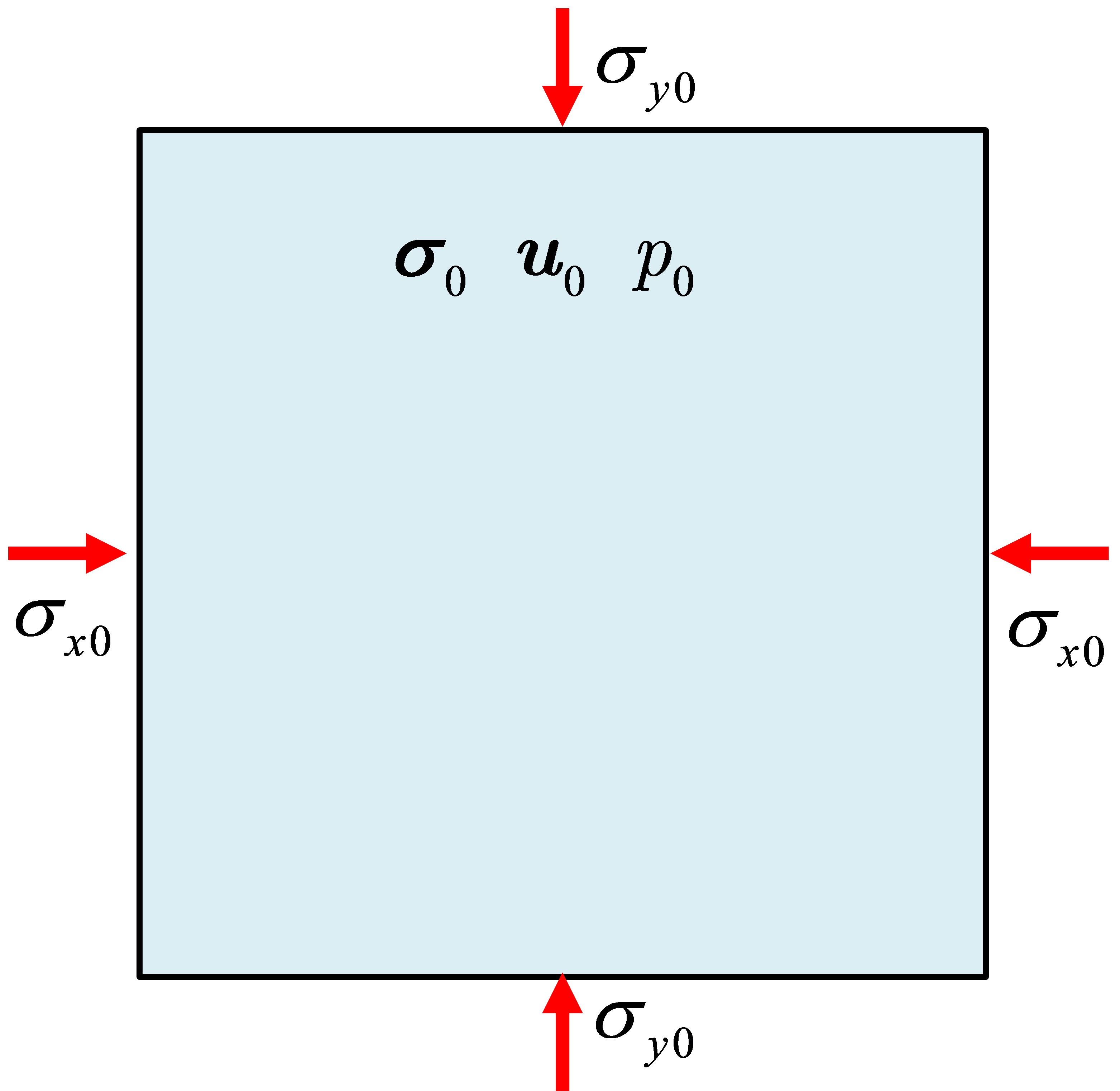
(a) Initial state

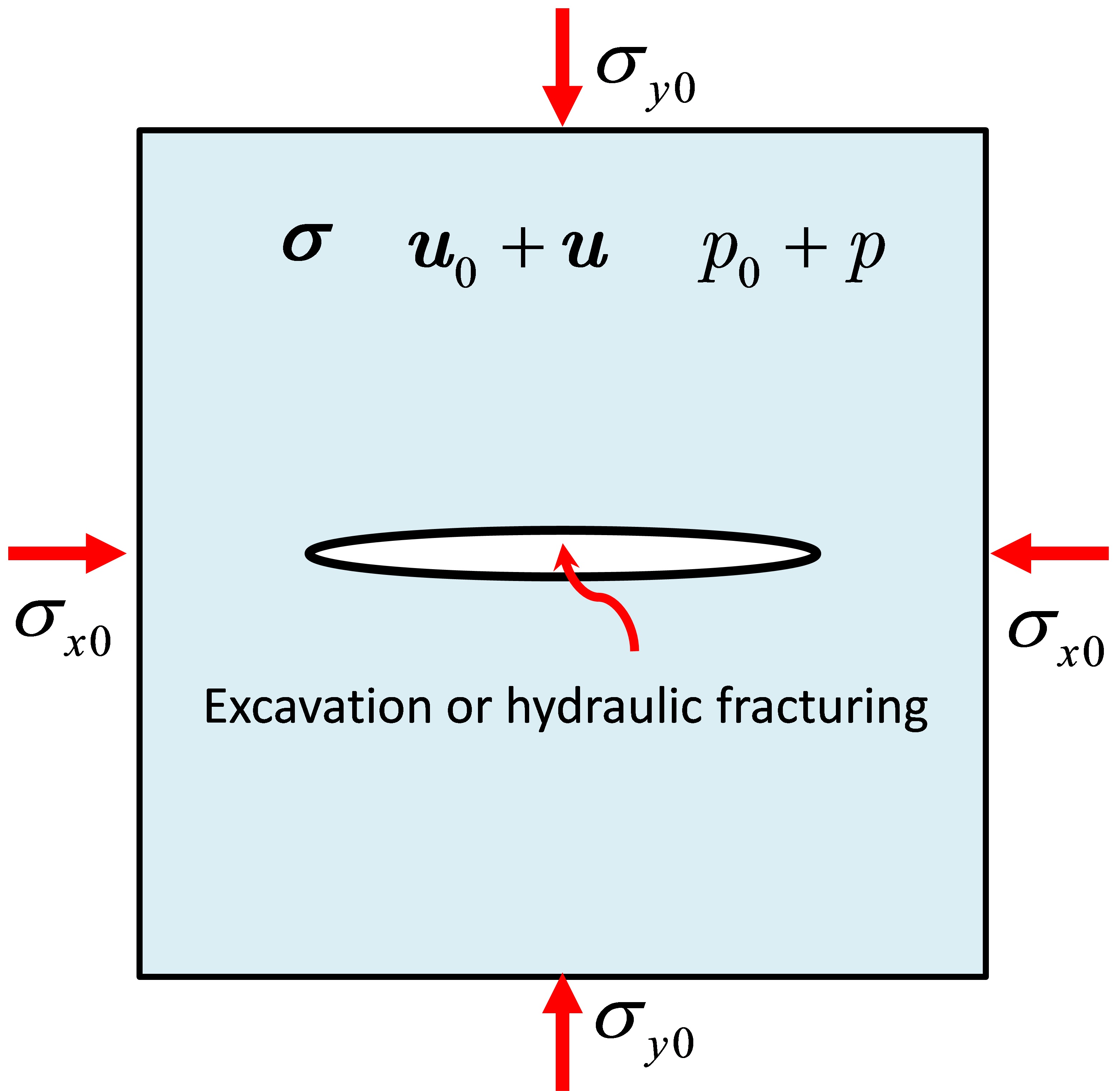
(b) After excavation or HF

Figure 2: Stress, displacement and fluid pressure in geological environment

If the body force is ignored, the basic idea of the previous phase field models for porous-elastic media [45] is to construct an energy functional $\Psi$ composed of the elastic energy $\Psi_{\varepsilon}(\bm{\varepsilon})$, fracture energy $\Psi_{f}$, external work $W_{ext}$, and the energy contribution of fluid pressure $p$:

$$\Psi(\bm{u},p,\Gamma)=\underbrace{\int_{\Omega\backslash\Gamma}\psi_{\varepsilon}(\bm{\varepsilon})\mathrm{d}{\Omega}}_{\Psi_{\varepsilon}}\underbrace{-\int_{\Omega}\alpha p\cdot(\nabla\cdot\bm{u})\mathrm{d}{\Omega}}_{\text{pressure-related term}}+\underbrace{\int_{\Gamma}G_{c}\mathrm{d}\Gamma}_{\Psi_{f}}\underbrace{-\int_{\partial\Omega_{t}}\bm{f}_{t}\cdot{\bm{u}}\mathrm{d}S}_{W_{ext}}$$ (1)

where $\psi_{\varepsilon}(\bm{\varepsilon})$ is the elastic energy density; $\alpha\in(0,1]$ is the Biot coefficient; $G_{c}$ is the critical energy release rate; $\bm{f}_{t}$ is the traction on the Neumann boundary on $\mathrm{d}S$. In addition, the linear strain tensor $\bm{\varepsilon}$ is given by

$$\varepsilon_{ij}=\frac{1}{2}\left(\frac{\partial u_{i}}{\partial x_{j}}+\frac{\partial u_{j}}{\partial x_{i}}\right)$$ (2)

and for an isotropic linear elastic medium, the elastic energy density $\psi_{\varepsilon}(\bm{\varepsilon})$ reads [20]

$$\psi_{\varepsilon}(\bm{\varepsilon})=\frac{1}{2}\lambda\varepsilon_{ii}\varepsilon_{jj}+\mu\varepsilon_{ij}\varepsilon_{ij}$$ (3)

where $\lambda,\mu>0$ are the Lamé constants and

$$\left\{\begin{aligned} \lambda&=\frac{E\nu}{(1+\nu)(1-2\nu)}\\ \mu&=\frac{E}{2(1+\nu)}\end{aligned}\right.$$ (4)

with $E$ and $\nu$ being Young’s modulus and Poisson’s ratio, respectively.

However, as seen in Eq.(1), the previously used energy functional cannot account for the effect of the initial stress field and it is therefore not suitable for modeling fracture propagation in a geomaterial under stress boundary condition. An evidence for this can be observed in Shiozawa et al. [46] where a stress boundary has a relatively large deformation when the fluid pressure is 0. Hence, to deal with the stress boundary and account for the effect of the initial stress field, we establish a new energy functional $L$ for the phase field modeling:

$$L(\bm{u},p,\Gamma)=\underbrace{\int_{\Omega\backslash\Gamma}\psi_{\varepsilon}(\bm{\varepsilon})\mathrm{d}{\Omega}}_{\Psi_{\varepsilon}}+\underbrace{\int_{\Omega\backslash\Gamma}\bm{\sigma}_{0}:\bm{\varepsilon}\mathrm{d}{\Omega}}_{\text{Initial stress induced}}\underbrace{-\int_{\Omega}\alpha p\cdot(\nabla\cdot\bm{u})\mathrm{d}{\Omega}}_{\text{pressure-related term}}+\underbrace{\int_{\Gamma}G_{c}\mathrm{d}\Gamma}_{\Psi_{f}}\underbrace{-\int_{\partial\Omega_{h}}\bm{f}_{t}\cdot{\bm{u}}\mathrm{d}S}_{W_{ext}}$$ (5)

where the sum of the first and second terms means the incremental elastic energy from the state of $\bm{u}_{0}$ to the state of $\bm{u}_{0}+\bm{u}$. It will be shown in the following sections that this incremental elastic energy drives the fracture propagation in the porous medium $\Omega$. In addition, it should be noted that by using the new energy functional (5), the fracture deflection phenomenon due to stress contrast can be also well captured by the phase field model, as shown in the numerical examples presented in this paper.

2.2 Phase field description

It can be seen from Eqs. (1) and (5) that the energy functional contains a sharp internal surface $\Gamma$, which increases the difficulty in minimizing the energy functional when the variational method is used. Therefore, to simplify the numerical implementation, a phase field $\phi(\bm{x},t)\in[0,1]$ is used to smear the sharp fracture as shown in Fig. 1b where $\phi=0$ and $\phi=1$ represent an intact material and a fully broken material, respectively.

For a fracture in a 1D bar, the solution for the phase field is an inverse exponential function $\phi(x)$ [20]:

$$\phi(x)=\mathrm{exp}\left(-\frac{|x-a|}{l_{0}}\right)$$ (6)

where $x=a$ is the fracture location and $l_{0}$ denotes the intrinsic length scale parameter. The length scale $l_{0}$ is also required for 2D and 3D problems where the crack surface density per unit volume is used in terms of the phase field and its gradient [20]:

$$\gamma(\phi,\bigtriangledown\phi)=\frac{\phi^{2}}{2l_{0}}+\frac{l_{0}}{2}\nabla\phi\cdot\nabla\phi$$ (7)

Note that the length scale parameter controls the width of a diffused fracture and a larger $l_{0}$ shows a lower nominal tensile strength in the phase field modeling [49]. Note that the sharp fracture can be recovered if $l_{0}$ tends to zero, which is known as $\Gamma$-convergence [20]. In addition, the length scale is assumed much larger than the pore size of the domain $\Omega$ in this study and therefore the fracture energy in Eq. (5) is rewritten as

$$\Psi_{f}=\int_{\Gamma}G_{c}\mathrm{d}\Gamma\approx\int_{\Omega}G_{c}\gamma\mathrm{d}\Omega=\int_{\Omega}G_{c}\left(\frac{\phi^{2}}{2l_{0}}+\frac{l_{0}}{2}|\nabla\phi|^{2}\right)\mathrm{d}\Omega$$ (8)

The elastic energy $\Psi_{\varepsilon}$ must be decomposed into tensile and compressive parts to ensure cracks only under tension [24]. Therefore, we follow the strain spectral decomposition of Miehe et al. [20]:

$$\bm{\varepsilon}_{\pm}=\sum_{a=1}^{d}\langle\varepsilon_{a}\rangle_{\pm}\bm{n}_{a}\otimes\bm{n}_{a}$$ (9)

where $\bm{\varepsilon}_{\pm}$ are the tensile and compressive strain tensors, respectively; $\varepsilon_{a}$ and $\bm{n}_{a}$ are the principal strain and its direction; the operators $\langle*\rangle_{\pm}$ are defined as [20]: $\langle*\rangle_{\pm}=(*\pm|*|)/2$.

Applying the decomposed strain tensor, the tensile and compressive parts of the elastic energy density are written as

$$\psi_{\varepsilon}^{\pm}(\bm{\varepsilon})=\frac{\lambda}{2}\langle\mathrm{tr}(\bm{\varepsilon})\rangle_{\pm}^{2}+\mu\mathrm{tr}\left(\bm{\varepsilon}_{\pm}^{2}\right)$$ (10)

We follow Borden et al. [24] and the compressive part of the elastic energy density is assumed not to affect the fracture propagation. Therefore, the elastic energy is rewritten as

$$\Psi_{\varepsilon}=\int_{\Omega\backslash\Gamma}\psi_{\varepsilon}(\bm{\varepsilon})\mathrm{d}{\Omega}=\int_{\Omega}\left[g(\phi)\psi_{\varepsilon}^{+}(\bm{\varepsilon})+\psi_{\varepsilon}^{-}(\bm{\varepsilon})\right]\mathrm{d}{\Omega}$$ (11)

where $g(\phi)$ is a degradation function, and $g(0)=1$, $g(1)=0$, $g^{\prime}(1)=0$ must be satisfied [23]. Although there are many forms for $g(\phi)$, a quadratic form of $g(\phi)=(1-k)(1-\phi)^{2}+k$ is applied in this work with $k=10^{-9}$ being a stability parameter to prevent numerical singularity when $\phi=0$.

The degradation function is also applied to the energy variation due to the initial stress field:

$$\int_{\Omega\backslash\Gamma}\bm{\sigma}_{0}:\bm{\varepsilon}\mathrm{d}{\Omega}\approx\int_{\Omega}g(\phi)\bm{\sigma}_{0}:\bm{\varepsilon}\mathrm{d}{\Omega}$$ (12)

which means the initial stress field does not contribute to the energy functional in a fully broken region with $\phi=0$.

2.3 Governing equations for the displacement

Now, substituting the fracture energy (8), the elastic energy (11), and Eq. (12) into Eq. (5), the energy functional can be rewritten as

$$L=\int_{\Omega}\left[g(\phi)\psi_{\varepsilon}^{+}(\bm{\varepsilon})+\psi_{\varepsilon}^{-}(\bm{\varepsilon})\right]\mathrm{d}{\Omega}+\int_{\Omega}g(\phi)\bm{\sigma}_{0}:\bm{\varepsilon}\mathrm{d}{\Omega}-\int_{\Omega}\alpha p\cdot(\nabla\cdot\bm{u})\mathrm{d}{\Omega}+\\ \int_{\Omega}G_{c}\left[\frac{\phi^{2}}{2l_{0}}+\frac{l_{0}}{2}\nabla\phi\cdot\nabla\phi\right]\mathrm{d}{\Omega}-\int_{\partial\Omega_{h}}\bm{f}_{t}\cdot\bm{u}\mathrm{d}S$$ (13)

We then apply the variational approach [50] where fracture initiation and propagation at time $t\in[0,T]$ is a process to minimize the energy functional $L$. Therefore, the first variation of the energy functional $L$ is set as 0, yielding

$$\delta L=\underbrace{\int_{\partial\Omega_{h}}\left[\left(\sigma_{ij}^{e}+g(\phi)\sigma_{0ij}-\alpha p\delta_{ij}\right)m_{j}-f_{ti}\right]\delta u_{i}\mathrm{d}{S}}_{①}-\underbrace{\int_{\Omega}\left(\sigma_{ij}^{e}+g(\phi)\sigma_{0ij}-\alpha p\delta_{ij}\right)_{,j}\delta u_{i}\mathrm{d}{\Omega}}_{②}-\\ \underbrace{\int_{\Omega}\left[g^{\prime}(\phi)(\psi_{\varepsilon}^{+}+\sigma_{0ij}\varepsilon_{ij})+\frac{G_{c}\phi}{l_{0}}-G_{c}l_{0}\frac{\partial^{2}\phi}{\partial x_{i}^{2}}\right]\delta\phi\mathrm{d}{\Omega}}_{③}+\underbrace{\int_{\partial\Omega}\left(\frac{\partial\phi}{\partial x_{i}}m_{i}\right)\delta\phi\mathrm{d}S}_{④}=0$$ (14)

where $g^{\prime}(\phi)=\mathrm{d}g(\phi)/\mathrm{d}\phi=2(\phi-1)(1-k)$ and $m_{j}$ is the component of the outward-pointing normal vector of the boundary. $\sigma_{ij}^{e}$ is the component of the effective stress tensor $\bm{\sigma}(\bm{\varepsilon})^{e}$ induced by the displacement $\bm{u}$:

$$\bm{\sigma}^{e} =g(\phi)\frac{\partial{\psi_{\varepsilon}^{+}}}{\partial{\bm{\varepsilon}}}+\frac{\partial{\psi_{\varepsilon}^{-}}}{\partial\bm{\varepsilon}}$$ (15)

$$=\left[(1-k)(1-\phi)^{2}+k\right]\left[\lambda\langle tr(\bm{\varepsilon})\rangle_{+}\bm{I}+2\mu\bm{\varepsilon}_{+}\right]+\lambda\langle tr(\bm{\varepsilon})\rangle_{-}\bm{I}+2\mu\bm{\varepsilon}_{-}$$

where $\bm{I}$ is the identity tensor $\in\mathbb{R}^{d\times d}$.

Now, we define the total stress tensor $\bm{\sigma}$ as

$$\bm{\sigma}(\bm{\varepsilon})=\bm{\sigma}^{e}(\bm{\varepsilon})+g(\phi)\bm{\sigma}_{0}-\alpha p\bm{I},\hskip 14.22636pt\mathrm{in}\hskip 2.84544pt\Omega\times(0,T]$$ (16)

Combining Eqs. (15) and (16), it can be seen that in a pure tension state without fluid, if the phase field $\phi=1$, the total stress $\bm{\sigma}$ is 0 in the fully broken region. In addition, because arbitrary admissible $\delta u$ must satisfy Eq. (14), Eq. (14)$②$ gives rise to the governing equation:

$$\frac{\partial{\sigma_{ij}}}{\partial x_{j}}=0,\hskip 14.22636pt\mathrm{in}\hskip 2.84544pt\Omega\times(0,T]$$ (17)

subjected to the Dirichlet boundary and the Neumann boundary given by

$$\sigma_{ij}m_{j}=f_{ti},\hskip 28.45274pt\mathrm{on}\hskip 14.22636pt\partial\Omega_{h}\times(0,T]$$ (18)

which can be derived from Eq. (14)$①$.

2.4 Governing equations for the phase field

Because of the arbitrariness of $\delta\phi$, Eq. (14)$③$ results in the original governing equation for the phase field:

$$\left[\frac{2l_{0}(1-k)(\psi_{\varepsilon}^{+}+\sigma_{0ij}\varepsilon_{ij})}{G_{c}}+1\right]\phi-l_{0}^{2}\frac{\partial^{2}\phi}{\partial{x_{i}^{2}}}=\frac{2l_{0}(1-k)(\psi_{\varepsilon}^{+}+\sigma_{0ij}\varepsilon_{ij})}{G_{c}},\hskip 14.22636pt\mathrm{in}\hskip 2.84544pt\Omega\times(0,T]$$ (19)

However, Eq. (19) cannot ensure the irreversibility condition $\Gamma(\bm{x},s)\in\Gamma(\bm{x},t)(s<t)$. Therefore, a history reference field $H$ is constructed to form a monotonically increasing phase field:

$$H(\bm{x},t)=\max\limits_{s\in[0,t]}\left[\psi_{\varepsilon}^{+}\left(\bm{\varepsilon}(\bm{x},s)\right)+\bm{\sigma}_{0}:\bm{\varepsilon}(\bm{x},s)\right],\hskip 14.22636pt\mathrm{in}\hskip 2.84544pt\Omega\times(0,T]$$ (20)

Replacing $\psi_{\varepsilon}^{+}+\sigma_{0ij}\varepsilon_{ij}$ by $H(\bm{x},t)$ in Eq. (19), the strong form for the phase field is given by

$$\left[\frac{2l_{0}(1-k)H}{G_{c}}+1\right]\phi-l_{0}^{2}\frac{\partial^{2}\phi}{\partial{x_{i}^{2}}}=\frac{2l_{0}(1-k)H}{G_{c}},\hskip 14.22636pt\mathrm{in}\hskip 2.84544pt\Omega\times(0,T]$$ (21)

which is subjected to the Neumann condition:

$$\frac{\partial\phi}{\partial x_{i}}m_{i}=0,\hskip 14.22636pt\mathrm{on}\hskip 14.22636pt\partial\Omega\times(0,T]$$ (22)

Therefore, the evolution equation of the phase field (21) indicates that the fracture initiation and propagation is driven by the history reference field $H(x,t)$, which represents the historic high incremental elastic energy from the $\bm{u}_{0}$ state to the $\bm{u}_{0}+\bm{u}$ state during the period $(0,t]$.

2.5 Fluid flow in the porous medium

As described in Subsection 2.1, the fluid in poro-elastic medium is assumed compressible and viscous. Then, we calculate the fluid flow in three subdomains, namely the unbroken domain (reservoir domain) $\Omega_{r}(t)$, fractured domain $\Omega_{f}(t)$ and transition domain $\Omega_{t}(t)$, respectively. These subdomains are distinguished according to the phase field in Table 1 where $c_{1}$ and $c_{2}$ are two phase field thresholds.

Table 1: Subdomain definition

Subdomain	Phase field
Reservoir domain	$\phi\leq c_{1}$
Transition domain	$c_{1}<\phi<c_{2}$
Fractured domain	$\phi\geq c_{2}$

In this study, we calculate the hydraulic parameters in the transition domain by using a linear interpolation from the reservoir and fractured domains. Therefore, two indicator functions $\chi_{r}$ and $\chi_{f}$ [46] are established. $\chi_{r}=1$ in the reservoir domain and $\chi_{r}=0$ in the fractured domain. In contrast, $\chi_{f}=0$ in the reservoir domain and $\chi_{f}=1$ in the fractured domain. In addition, the indicator functions satisfy the following:

$$\left\{\begin{aligned} &\chi_{r}(\cdot,\phi)=\frac{c_{2}-\phi}{c_{2}-c_{1}}\hskip 28.45274pt&c_{1}<\phi<c_{2}\\ &\chi_{f}(\cdot,\phi)=\frac{\phi-c_{1}}{c_{2}-c_{1}}\hskip 28.45274pt&c_{1}<\phi<c_{2}\end{aligned}\right.$$ (23)

Darcy’s law is used to model the fluid flow and the mass conservation equation in Zhou et al. [45] is applied to the whole calculation domain:

$$\rho S\frac{\partial p}{\partial t}+\nabla\cdot(\rho\bm{v})=q_{m}-\rho\alpha\chi_{r}\frac{\partial\varepsilon_{vol}}{\partial t}$$ (24)

where $\rho$, $S$, $\bm{v}$, $\varepsilon_{vol}=\nabla\cdot\bm{u}$, and $q_{m}$ represent the fluid density, storage coefficient, flow velocity, volumetric strain, and fluid source term, respectively. In Eq. (24), $\rho=\rho_{r}\chi_{r}+\rho_{f}\chi_{f}$ and $\alpha=\alpha_{r}\chi_{r}+\alpha_{f}\chi_{f}$ where $\rho_{r}$ and $\rho_{f}$ are the fluid densities in the reservoir and fracture domains while $\alpha_{r}$ and $\alpha_{f}$ are the Biot coefficients of the reservoir and fractured domains. Naturally, $\alpha_{f}=1$ is set for the fractured domain and therefore $\alpha=\alpha_{r}\chi_{r}+\chi_{f}$.

In Eq. (24), the storage coefficient $S$ is expressed as [45]

$$S=\varepsilon_{p}c+\frac{(\alpha-\varepsilon_{p})(1-\alpha)}{K_{Vr}}$$ (25)

where $\varepsilon_{p}$, $c$, and $K_{Vr}$ are the porosity, fluid compressibility, and bulk modulus of the calculation domain, respectively. Denoting $c_{r}$ and $c_{f}$ as the fluid compressibility in the reservoir and fractured domains, we have $c=c_{r}\chi_{r}+c_{f}\chi_{f}$.

The gravity is not considered in this study; therefore the Darcy’s velocity $\bm{v}$ is calculated as

$$\bm{v}=-\frac{K_{eff}}{\mu_{eff}}\nabla p$$ (26)

where $\mu_{eff}$ denotes fluid viscosity. Similarly, $\mu_{eff}=\mu_{r}\chi_{r}+\mu_{f}\chi_{f}$ with $\mu_{r}$ and $\mu_{f}$ being the fluid viscosity in the reservoir and fractured domains, respectively. $K_{eff}$ is the effective permeability and $K_{eff}=k_{r}\chi_{r}+k_{f}\chi_{f}$ where $k_{r}$ and $k_{f}$ are the permeabilities of the reservoir and fractured domains. Replacing Eq. (26) into Eq. (24), the governing equation for fluid flow is expressed in terms of the fluid pressure $p$:

$$\rho S\frac{\partial p}{\partial t}-\nabla\cdot\frac{\rho K_{eff}}{\mu_{eff}}\nabla p=q_{m}-\rho\alpha\chi_{r}\frac{\partial\varepsilon_{vol}}{\partial t}$$ (27)

which is subjected to the Dirichlet condition on $\partial\Omega_{D}$ and Neumann condition on $\partial\Omega_{N}$ [45]:

$$\left\{\begin{aligned} &p=p_{D}\hskip 56.9055pt&\mathrm{on}\quad\partial\Omega_{D}\\ &-\bm{n}\cdot\rho\bm{v}=M_{N}\hskip 56.9055pt&\mathrm{on}\quad\partial\Omega_{N}\end{aligned}\right.$$ (28)

where $p_{D}$ and $M_{N}$ are the prescribed pressure and mass flux.

3 Numerical algorithm

We implement the proposed phase field model in the framework of finite element method (FEM) and the FE discretization can be seen in Appendix. In addition, a finite difference method is applied for the time discretization. The overall procedure of our numerical algorithm for solving the three fields is shown in Fig. 3 where a staggered scheme is used. That is, the three fields are solved sequentially and independently in each time step.

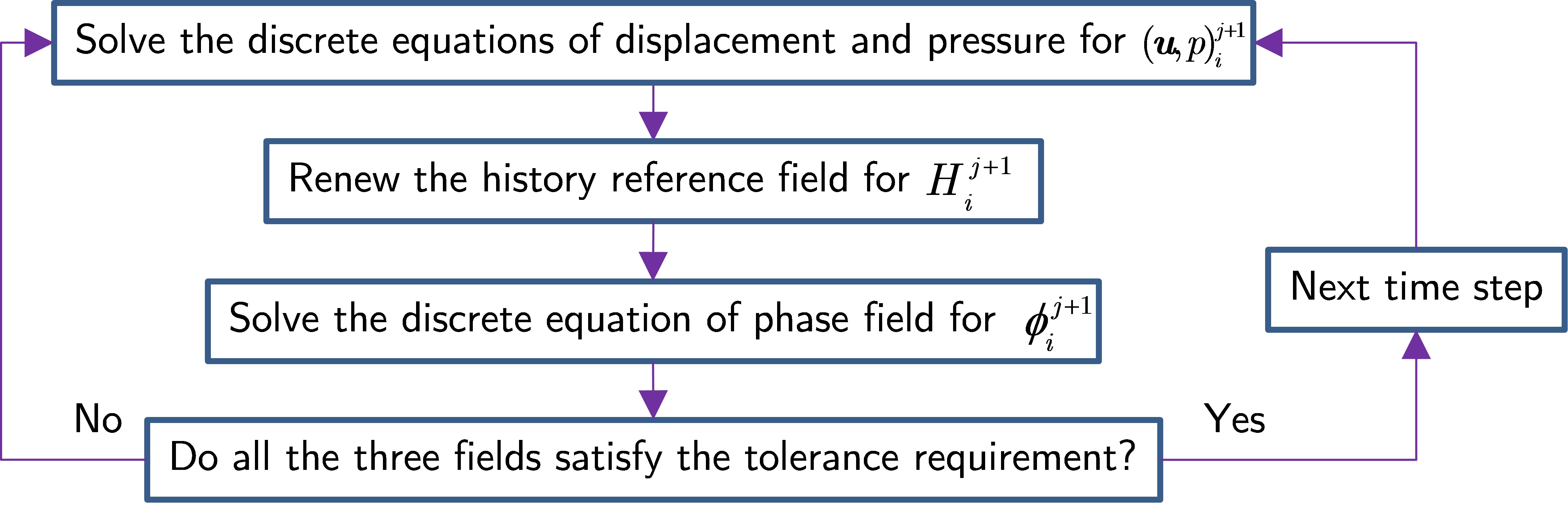
Figure 3: Numerical scheme in each time step

To reduce the computational effort, we implement the numerical method in the commercial software, COMSOL Multiphysics, which has been proven to have high capability for multi-field problems. In all simulations, the maximum iteration number is set as 150 due to high nonlinearity resulting from the derivative $\partial\bm{\sigma}^{e}/\partial\bm{\varepsilon}$ and the phase field which degrades the stiffness matrix of the displacement field. In addition, a stabilization and convergence acceleration method–the Anderson acceleration technique is applied. For more detail on the COMSOL implementation, the readers can be referred to the previous study [51].

4 2D examples

In this section, 2D examples of specimens subjected to internal fluid injection are presented to prove the capability of the proposed phase field method. All the pre-existing cracks are established by introducing an initial history field with a relatively high $H$ [24] and the source term in the pre-existing notches is set as $q_{F}=10$ kg/(m${}^{3}\cdot$s) in all examples.

4.1 Fractures from a horizontal notch

The first example tests the hydraulic fracture propagation from a horizontal notch in a square domain. The geometry and boundary conditions of this example are shown in Fig. 4 with increasing fluid volume in the initial notch. All the outer boundaries of the calculation domain has a fluid pressure of $p=0$ and a zero tangential displacement in order to remove the effect of rigid body displacement. In addition, the parameters for calculation are listed in Table 2.

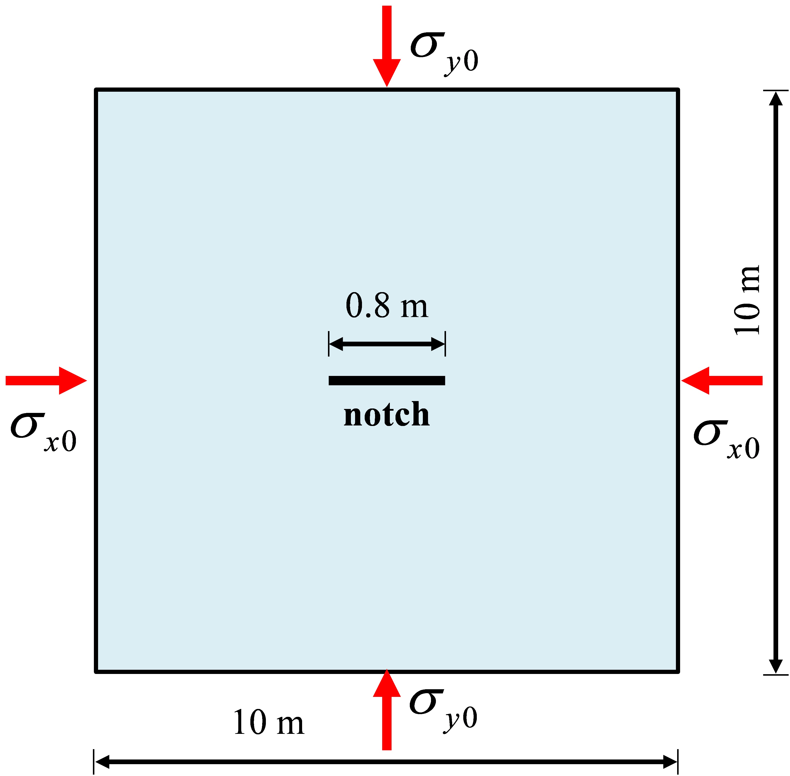
Figure 4: Geometry and boundary conditions of the calculation domain

Table 2: Basic calculation parameters

Parameter	Value	Unit	Parameter	Value	Unit
$\mu$	23.08	GPa	$\lambda$	34.62	GPa
$G_{c}$	500	N/m	$k$	$1\times 10^{-9}$	–
$l_{0}$	0.1	m	$c_{1}$	0.4	–
$c_{2}$	1.0	–	$\varepsilon_{pR}$	0.05	–
$\rho_{R}$, $\rho_{F}$	$1.0\times 10^{3}$	kg/m3	$\alpha_{R}$	0.05	–
$q_{R}$	0	kg/(m${}^{3}\cdot$s)	$q_{F}$	0	kg/(m${}^{3}\cdot$s)
$k_{R}$	$1\times 10^{-15}$	m2	$k_{F}$	$8.333\times 10^{-4}$	m2
$c_{R}$	$1\times 10^{-8}$	1/Pa	$c_{F}$	$1\times 10^{-8}$	1/Pa
$\mu_{R}$	$1\times 10^{-3}$	Pa$\cdot$s	$\mu_{F}$	$1\times 10^{-3}$	Pa$\cdot$s

We discretize the calculation domain with unstructured triangular elements with the maximum element size $h=0.05$ m. Therefore, the linear shape functions are used for all the three physical fields. In addition, the time step $\Delta t=0.05$s is adopted for the simulation. The initial stress state of $\sigma_{x0}=0.5$ MPa, $\sigma_{y0}=0.5$ MPa and $\sigma_{z0}=\nu(\sigma_{x0}+\sigma_{y0})$ is applied with $\nu$ being Poisson’s ratio, which can be evaluated through the well-known elasticity relationship from $\lambda$ and $\mu$. As a comparison, we also model the fracture propagation by using the previously developed method [45] without considering the effect of initial stress field.

Figures 5 and 6 show the fracture propagation obtained by using the proposed phase field method and that without considering the effect of initial stress field. The figures indicate that discarding the effect of initial stress does not affect the fracture pattern for the first example; in both situation the fracture propagates along the horizontal direction. However, the time for fracture initiation and propagation is different and the fracture length is smaller if the initial stress field is considered in the constitutive model.

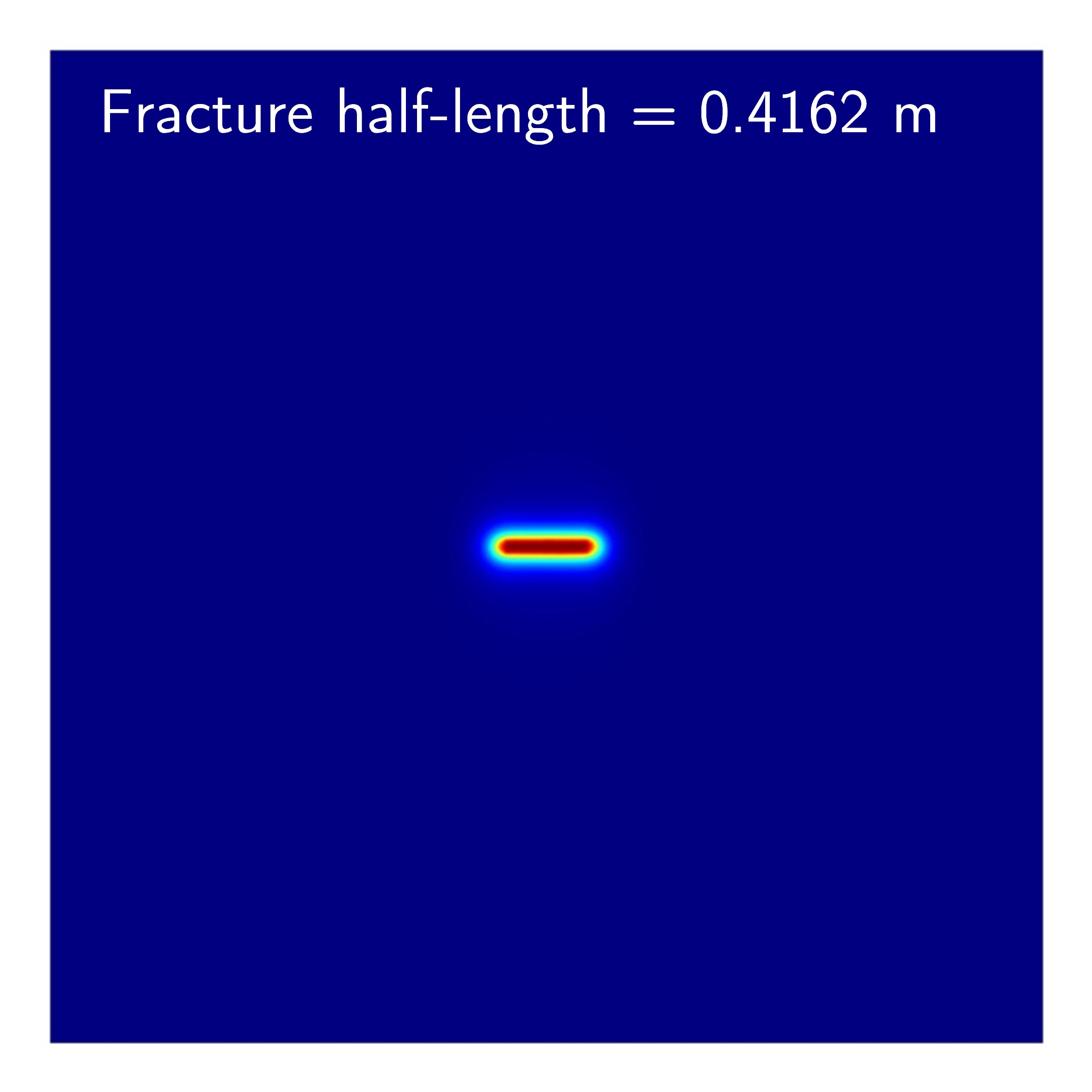
(a) $t=2.4$ s

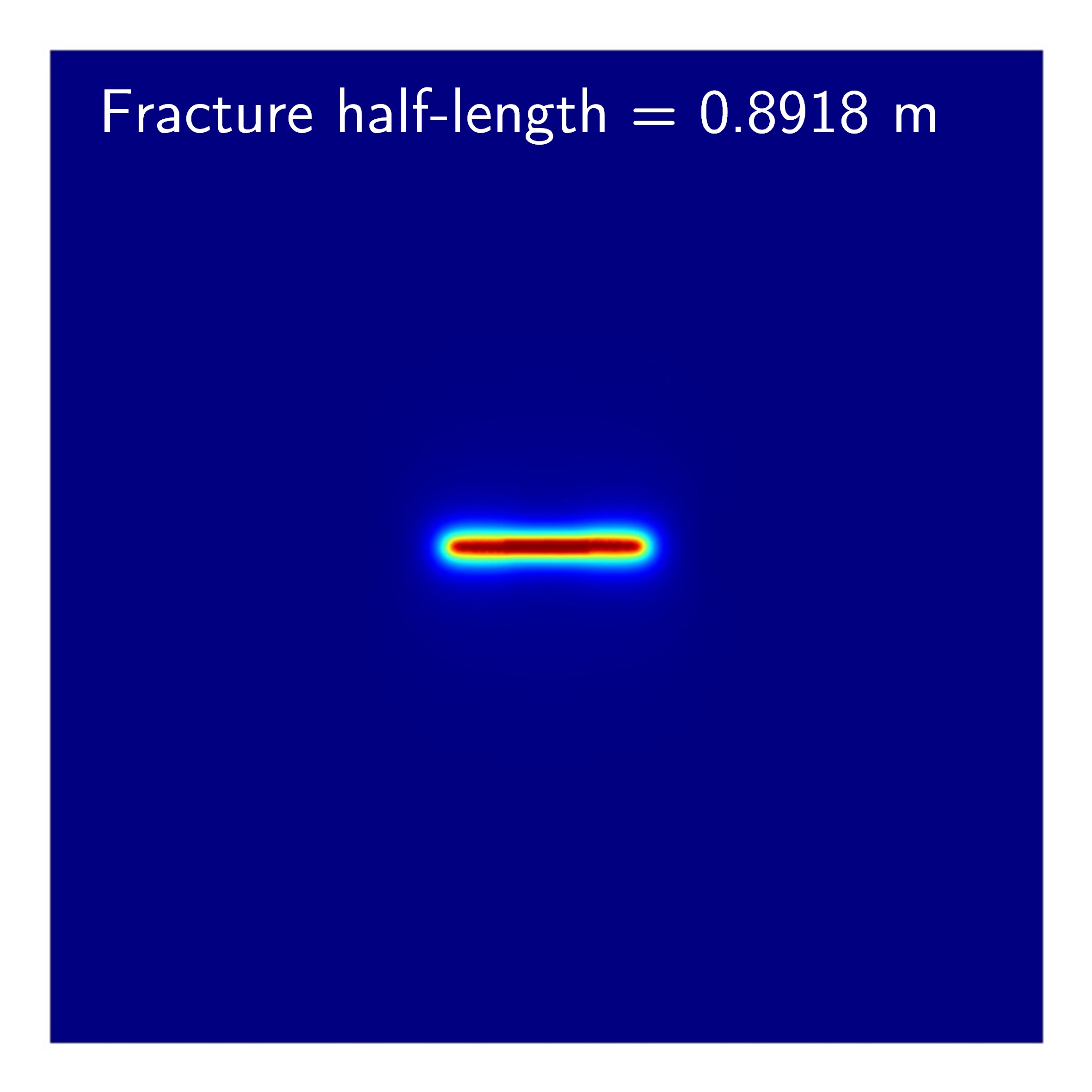
(b) $t=3.6$ s

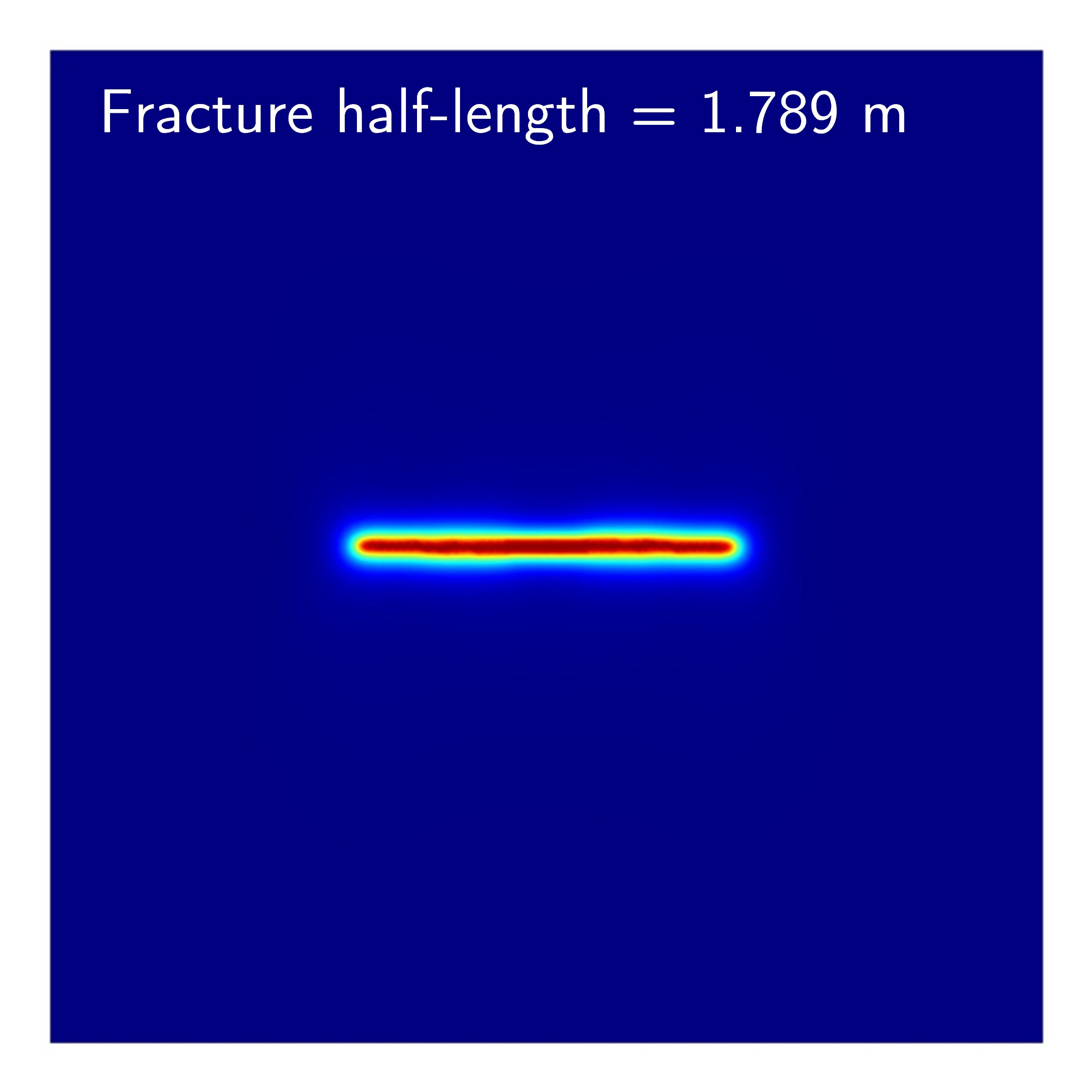
(c) $t=4.8$ s

Figure 5: Fracture propagation pattern by using the proposed PFM

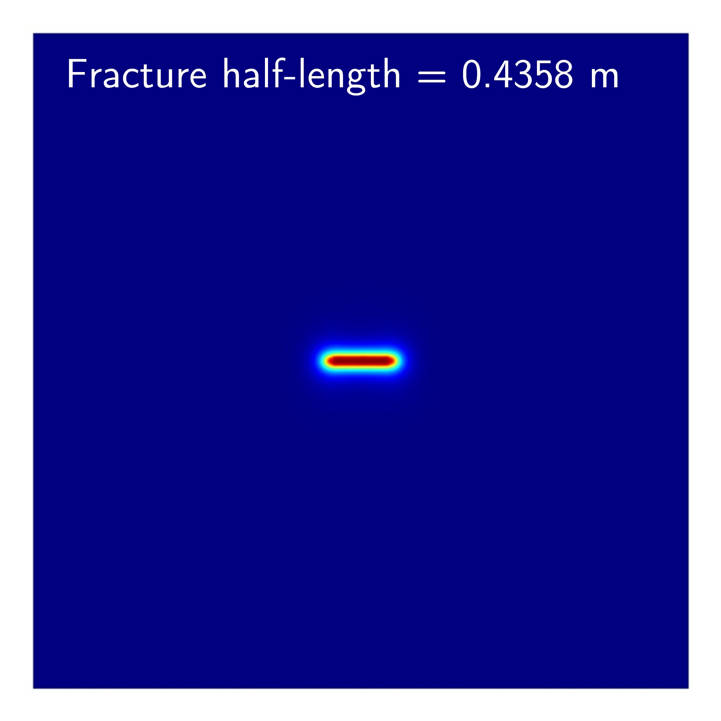
(a) $t=2.4$ s

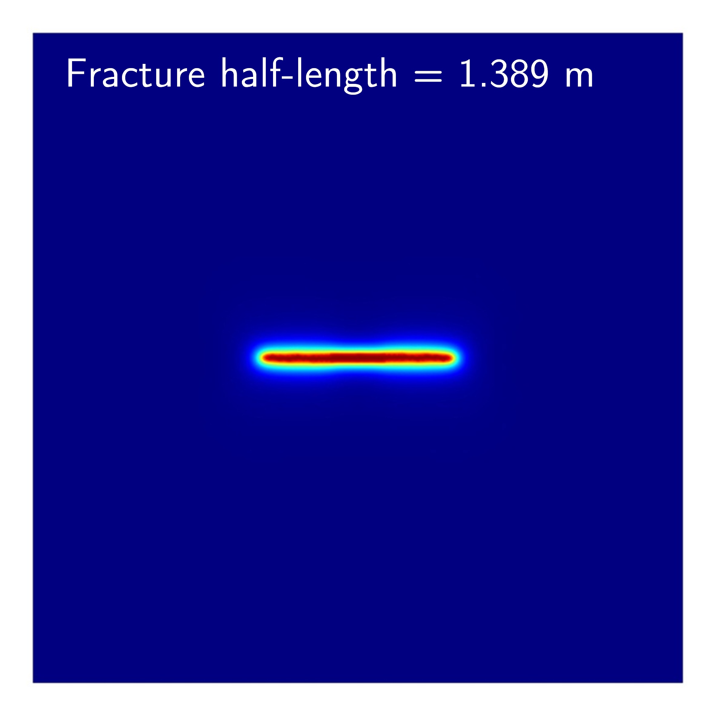
(b) $t=3.6$ s

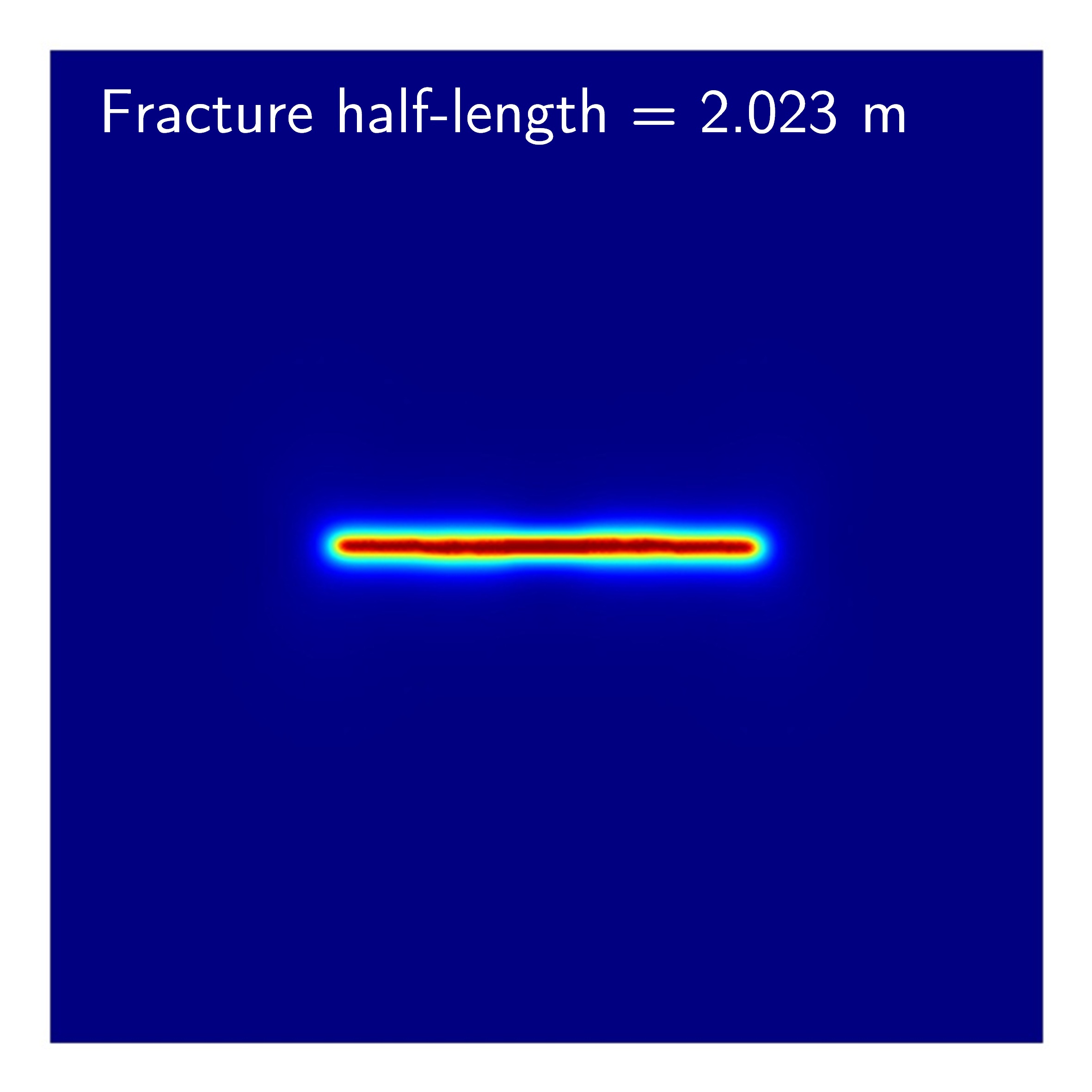
(c) $t=4.8$ s

Figure 6: Fracture propagation pattern without considering the effect of initial stress field

The displacement field at time $t=0$ s is shown in Fig. 7 where the region of $\phi\geq 0.95$ is removed to reflect the shape of the fully broken domain. It can be observed that the proposed PFM and the method of Zhou et al. [45] achieve different initial displacement field for the problem of a poro-elastic domain subjected to stress boundary condition. Fig. 7a indicates that only a small displacement appear around the center of the notch for the proposed PFM because the “excavation” or stiffness degradation of the initial notch produces displacement towards the broken domain. However, if the PFM does not consider the effect of initial stress field, all the outer boundaries have rather large displacements as shown in Fig. Fig. 7b. In addition, Fig. 8 compares the displacements along the top and left boundaries at time $t=0$ s. As observed, for the method of Zhou et al. [45], the stress boundary condition produces large initial displacements along the left and top boundaries while the initial displacement on the boundaries is negligible by using the proposed PFM. In summary, comparisons in Figs. 7 and 8 indicate the proposed PFM will achieve better displacement distribution compared with those PFMs without considering the effect of initial stress field, especially for the poro-elastic medium subjected to stress boundary condition in the geological environment.

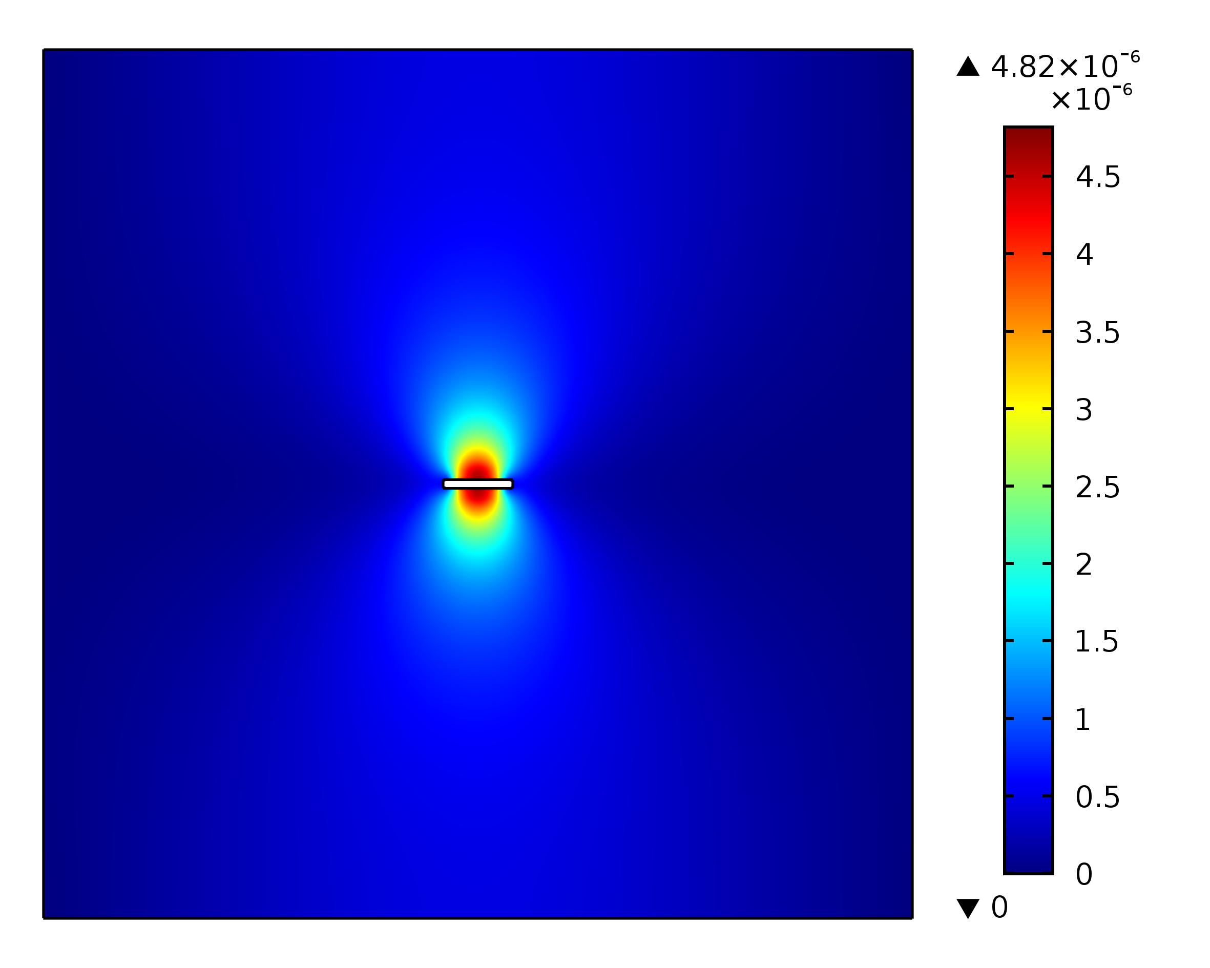
(a) The proposed PFM

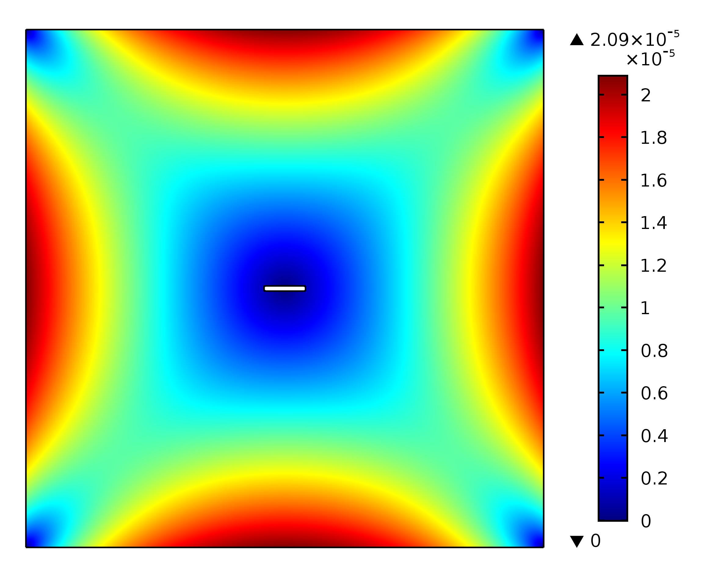
(b) Without considering the initial stress field

Figure 7: Comparison of the displacement field at $t=0$ s for the proposed PFM and Zhou et al. [45] (Unit: m)

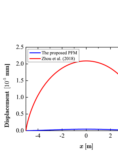
(a) Top boundary

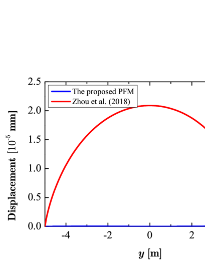
(b) Left boundary

Figure 8: Comparison of the displacement along the top and left boundaries at $t=0$ s for the proposed PFM and Zhou et al. [45]

Figure 9 shows the effect of initial stress field on the fluid pressure-time curve. Note that the data at the center of the initial notch are selected. Similar to the fracture pattern, Fig. 9 indicates the fluid pressure is only slightly affected by the initial stress field. In the current example, the time for fracture initiation is reduced if the initial stress field is not considered; therefore the fluid pressure-time curve has a earlier drop stage and a lower maximum pressure compared with those obtained by the proposed PFM as shown in Fig. 9.

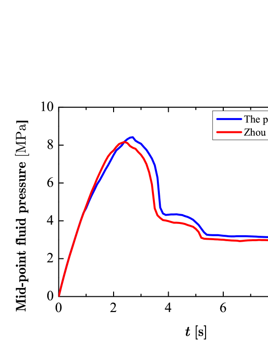
Figure 9: Comparison of the fluid pressure-time curve for the proposed PFM and Zhou et al. [45]

The evolution of the displacement field obtained by the proposed PFM is shown in Fig. 10. As expected, the maximum displacement occurs in the center of the fracture and it increases with the increasing time. This phenomenon is also consistent with those observations in a porous medium with fixed displacement boundaries [52; 36; 45], which indirectly reflects the applicability of the proposed PFM in this study.

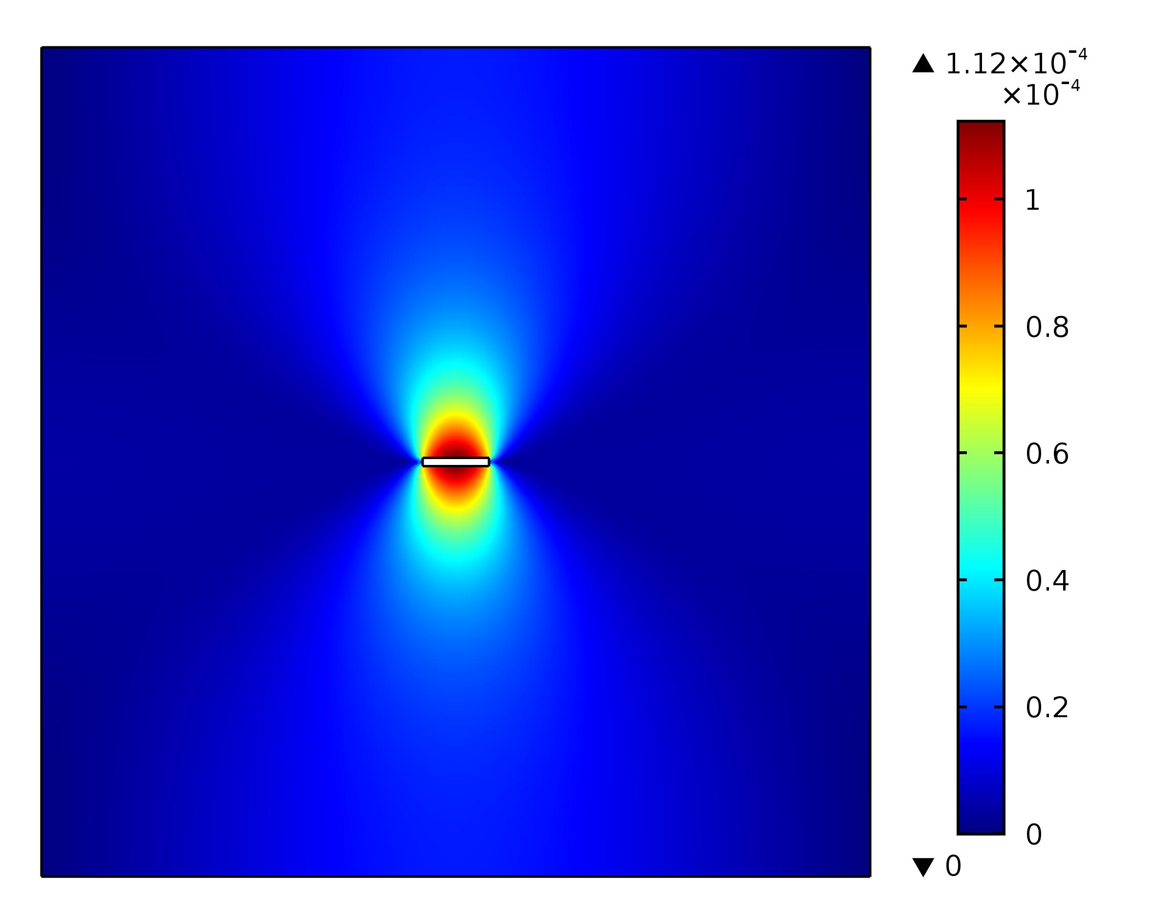
(a) $t=2.4$ s

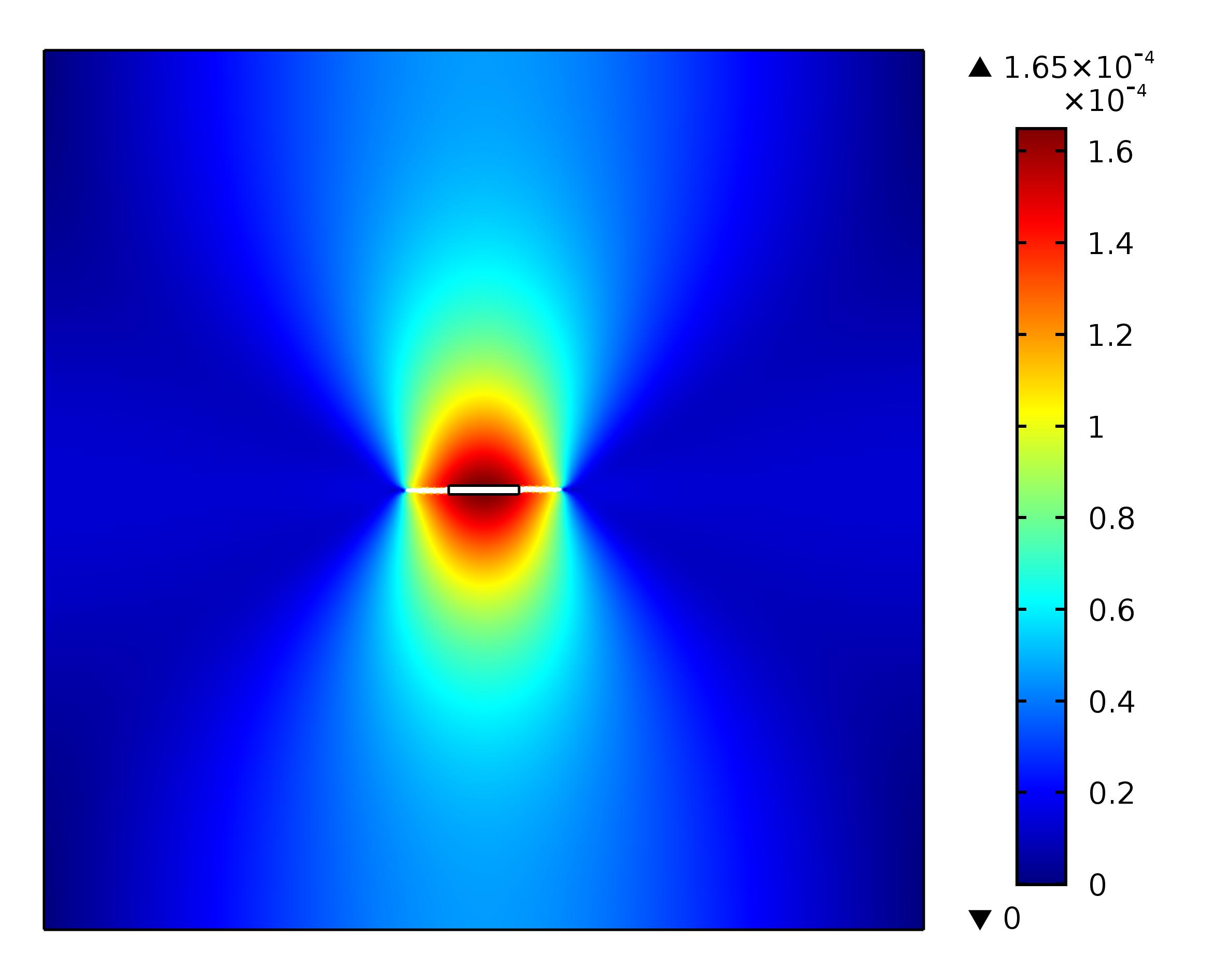
(b) $t=3.6$ s

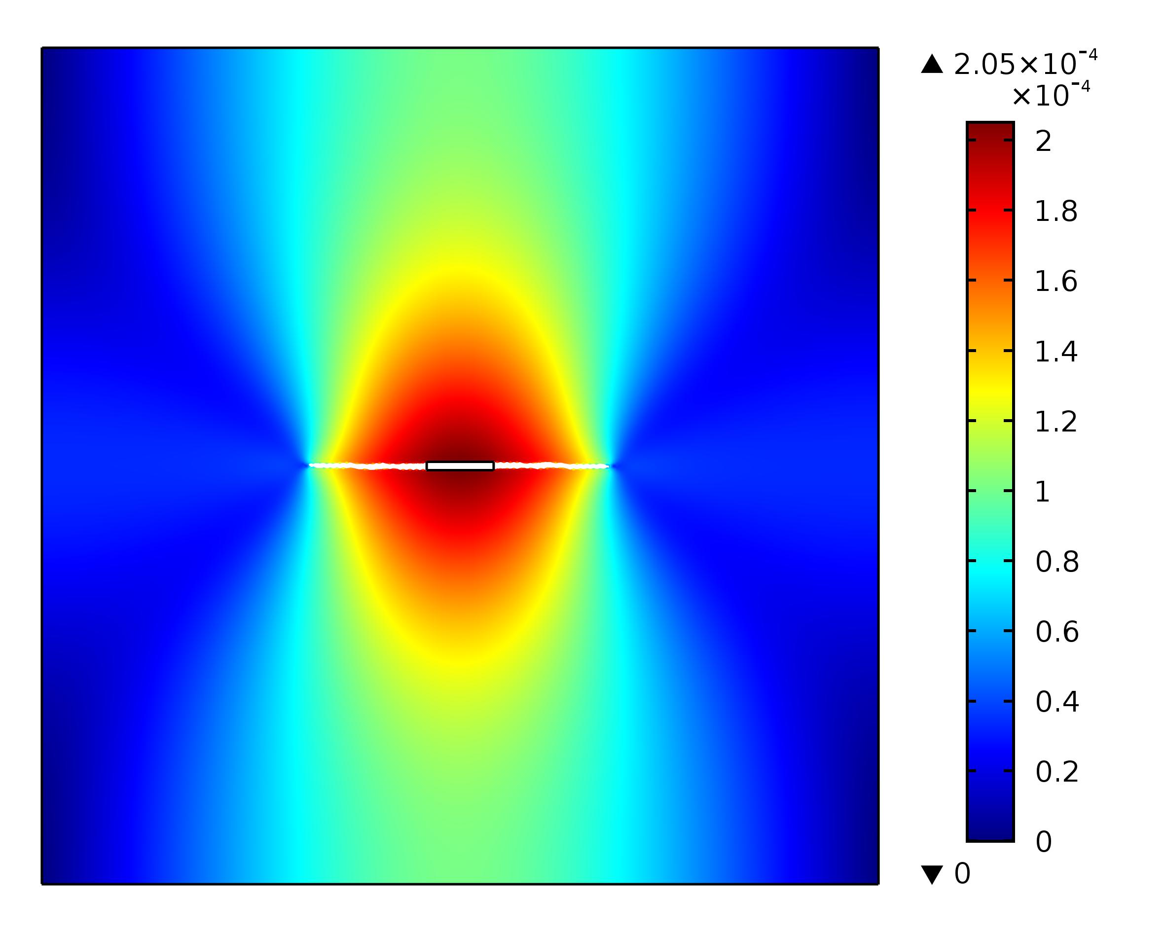
(c) $t=4.8$ s

Figure 10: Evolution of the displacement field by using the proposed PFM (Unit: m)

It is well-known that the hydraulic fracture pattern is highly affected by the stress contrast acting on the outer boundaries of the calculation domain. Therefore, in this example, we change the ratio of $\sigma_{y0}/\sigma_{x0}$ to $[0.5,1,2,10]$ with $\sigma_{x0}=0.5$ MPa unchanged to demonstrate the effect of stress contrast. By using the proposed PFM, the calculated fracture paths at time $t=10$ s are shown in Fig. 11. It can be observed that for $\sigma_{y0}/\sigma_{x0}=$ 0.5, 1, and 2, the fracture from the initial notch propagates horizontally and the fracture length decreases as the ratio of $\sigma_{y0}/\sigma_{x0}$ increases. However, when $\sigma_{y0}/\sigma_{x0}=10$, the fracture deflects and propagates along the direction of the maximum in-situ stress $S_{max}$, which is consistent with the engineering observations in hydraulic fracturing. In addition, the effect of the ratio of $\sigma_{y0}/\sigma_{x0}$ on the fluid pressure-time curve is shown in Fig. 12. The maximum fluid pressure at the mid-point of the initial notch is observed to increase with the increasing $\sigma_{y0}/\sigma_{x0}$.

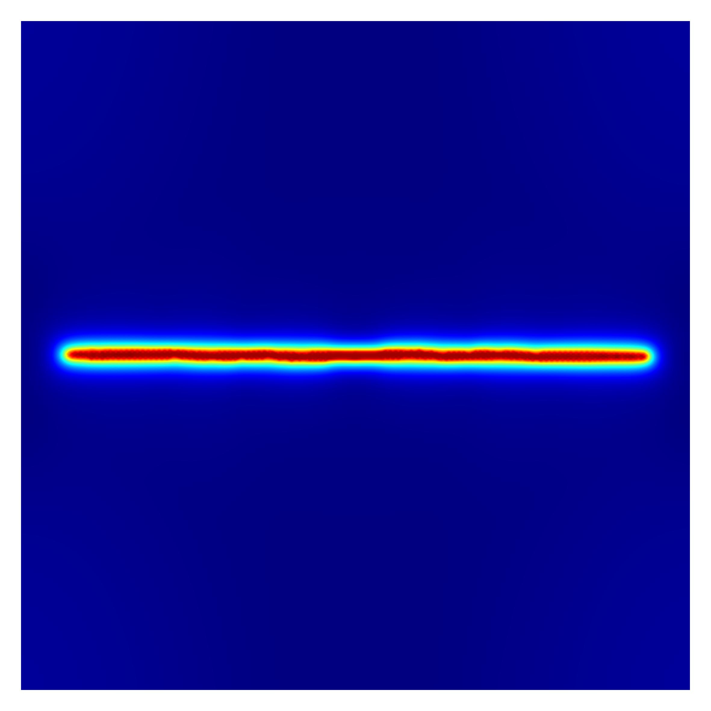
(a) $\sigma_{y0}/\sigma_{x0}=0.5$

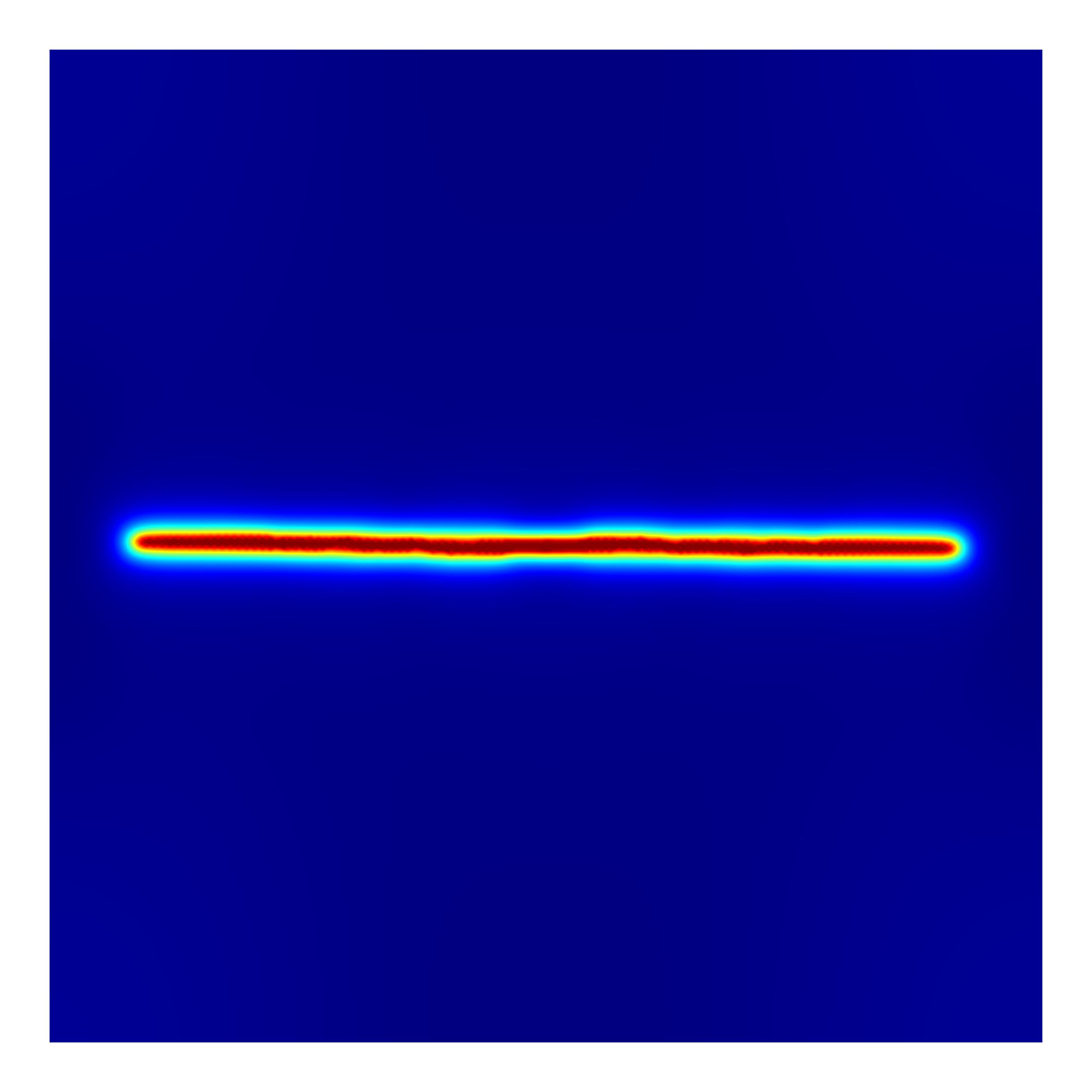
(b) $\sigma_{y0}/\sigma_{x0}=1$

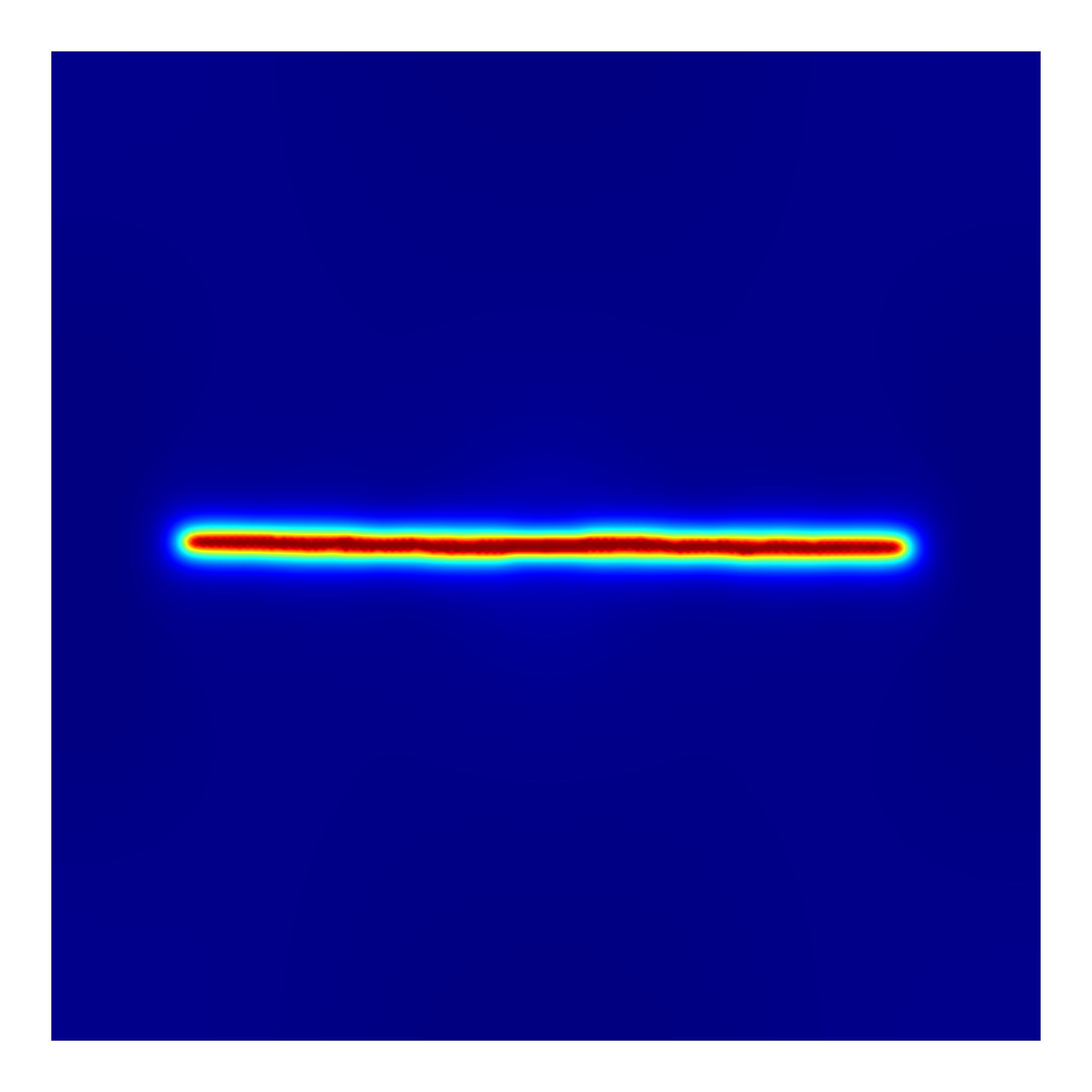
(c) $\sigma_{y0}/\sigma_{x0}=2$

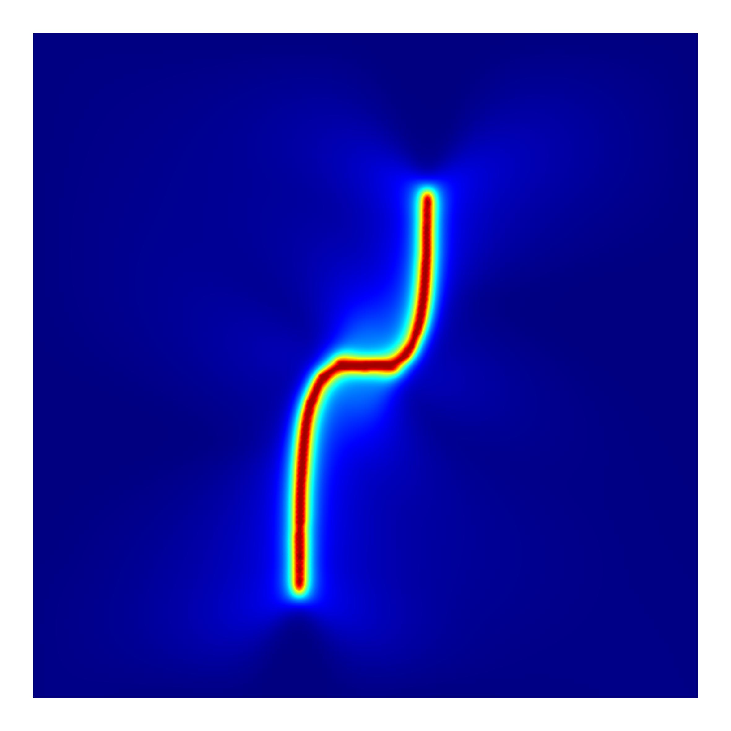
(d) $\sigma_{y0}/\sigma_{x0}=10$

Figure 11: Fracture propagation from a horizontal initial notch at time $t=10$ s under different $\sigma_{y0}/\sigma_{x0}$

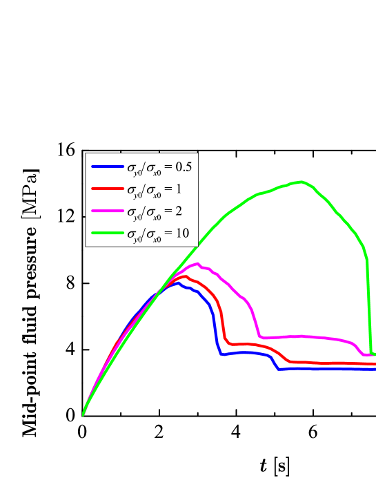
Figure 12: Effect of the ratio of $\sigma_{y0}/\sigma_{x0}$ on fluid pressure-time curve for a horizontal initial notch

Figure 13 describes the relative incremental mid-point fluid pressure and effective stress at fracture tip under different $\sigma_{y0}/\sigma_{x0}$ in the case of a horizontal initial notch. Note that the effective stress along the $y$ direction is accordingly used to show the effect of $\sigma_{y0}$, and the case of $\sigma_{y0}/\sigma_{x0}=0.5$ is used as the reference. As shown in Fig. 13, when the vertical stress $\sigma_{y0}$ increases linearly, the mid-point fluid pressure and effective stress at the fracture tip also increase linearly. This phenomena indirectly verifies the feasibility and practicability of the proposed PFM. Furthermore, the incremental fluid pressure is slightly larger than the vertical stress variation while the incremental effective stress at fracture tip is slightly lower.

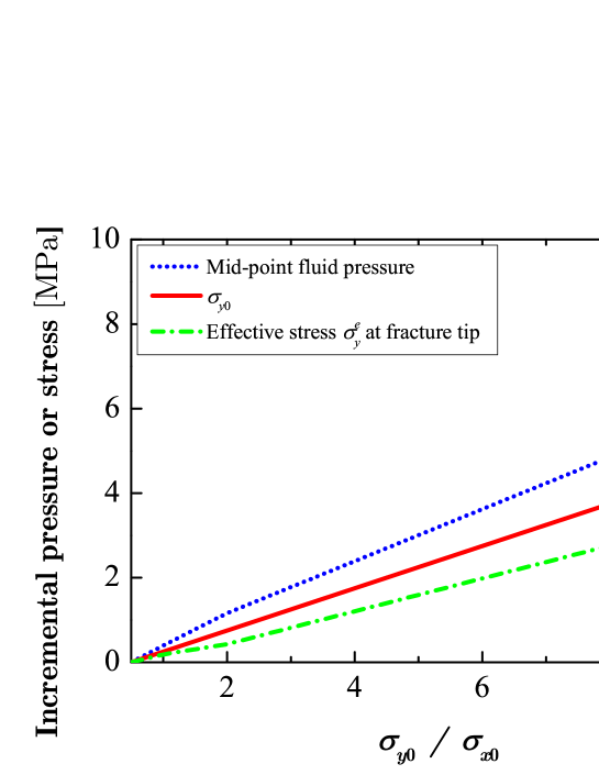
Figure 13: Relative incremental fluid pressure and effective stress at fracture tip under different $\sigma_{y0}/\sigma_{x0}$ in the case of a horizontal initial notch

4.2 Fracture from an inclined notch

We now consider an inclined initial notch in the calculation domain in Fig. 4. The notch has an length of 0.8 m and an inclination angle $\theta=45^{\circ}$ while the other simulation settings are the same as those in Subsection 4.1. Stress contrast $\sigma_{x0}/\sigma_{y0}=[1,2,4,6,8,10]$ is applied with the vertical stress $\sigma_{y0}=0.5$ MPa unchanged. Therefore, there are six simulations performed to show the effect of stress contrast on the fracture propagation from the inclined notch.

By using the proposed PFM, the phase field distribution for different $\sigma_{x0}/\sigma_{y0}$ at time $t=6$ s is shown in Fig. 14. As observed, the fracture propagates straight along the direction of the initial notch when $\sigma_{x0}/\sigma_{y0}=1$ at time $t=6$ s; however, if the stress ratio is larger than 1, the fracture deflects from the direction of the notch ($\theta=45^{\circ}$). All the simulations consistently indicate that the larger the ratio of $\sigma_{x0}/\sigma_{y0}$ is, the smaller angle the deflected fracture has from the direction of the maximum in-situ stress $S_{max}$ ($\sigma_{x0}$) in this example. The fluid pressure-time curve for different $\sigma_{x0}/\sigma_{y0}$ is shown in Fig. 15. Because the minimum in-situ stress $\sigma_{y0}$ is kept constant, the fluid pressure at the center of the notch only increases slightly with the increasing stress contrast $\sigma_{x0}/\sigma_{y0}$.

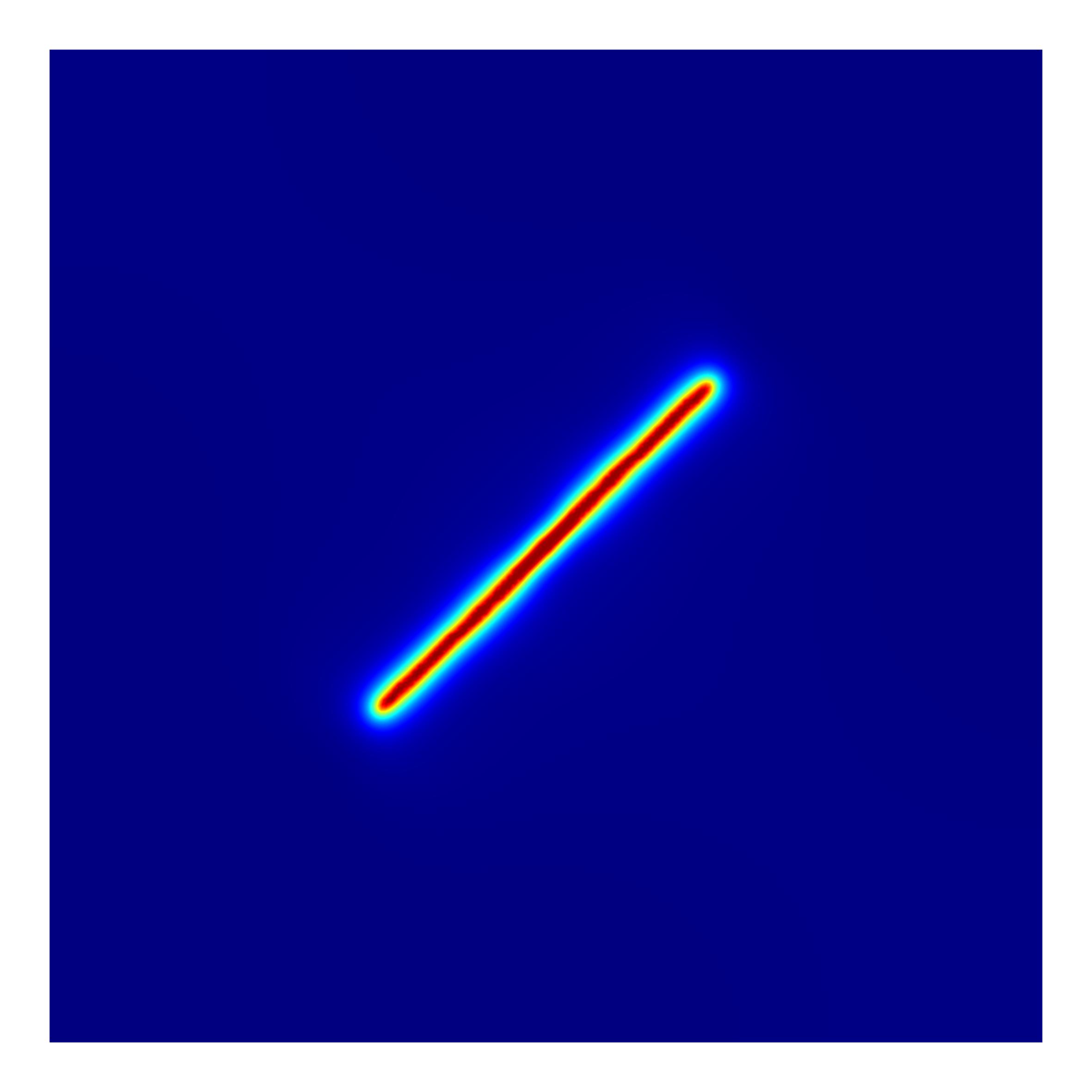
(a) $\sigma_{x0}/\sigma_{y0}=1$

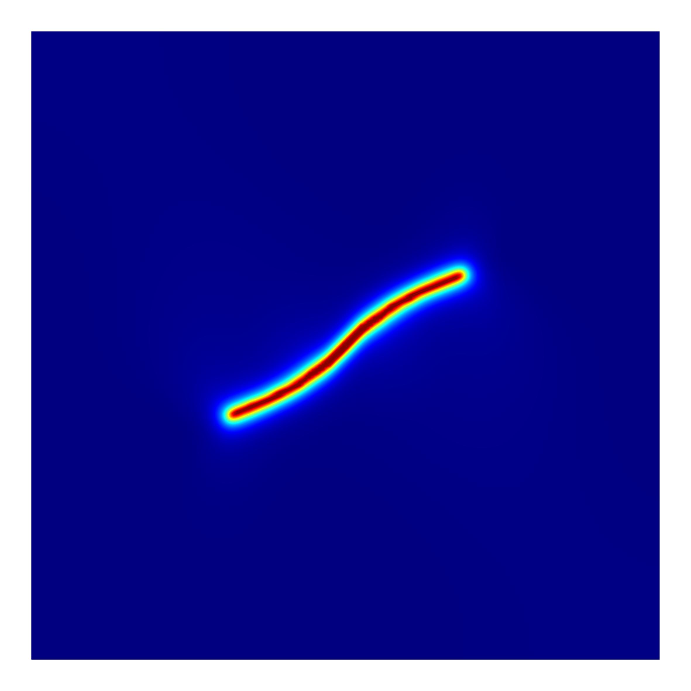
(b) $\sigma_{x0}/\sigma_{y0}=2$

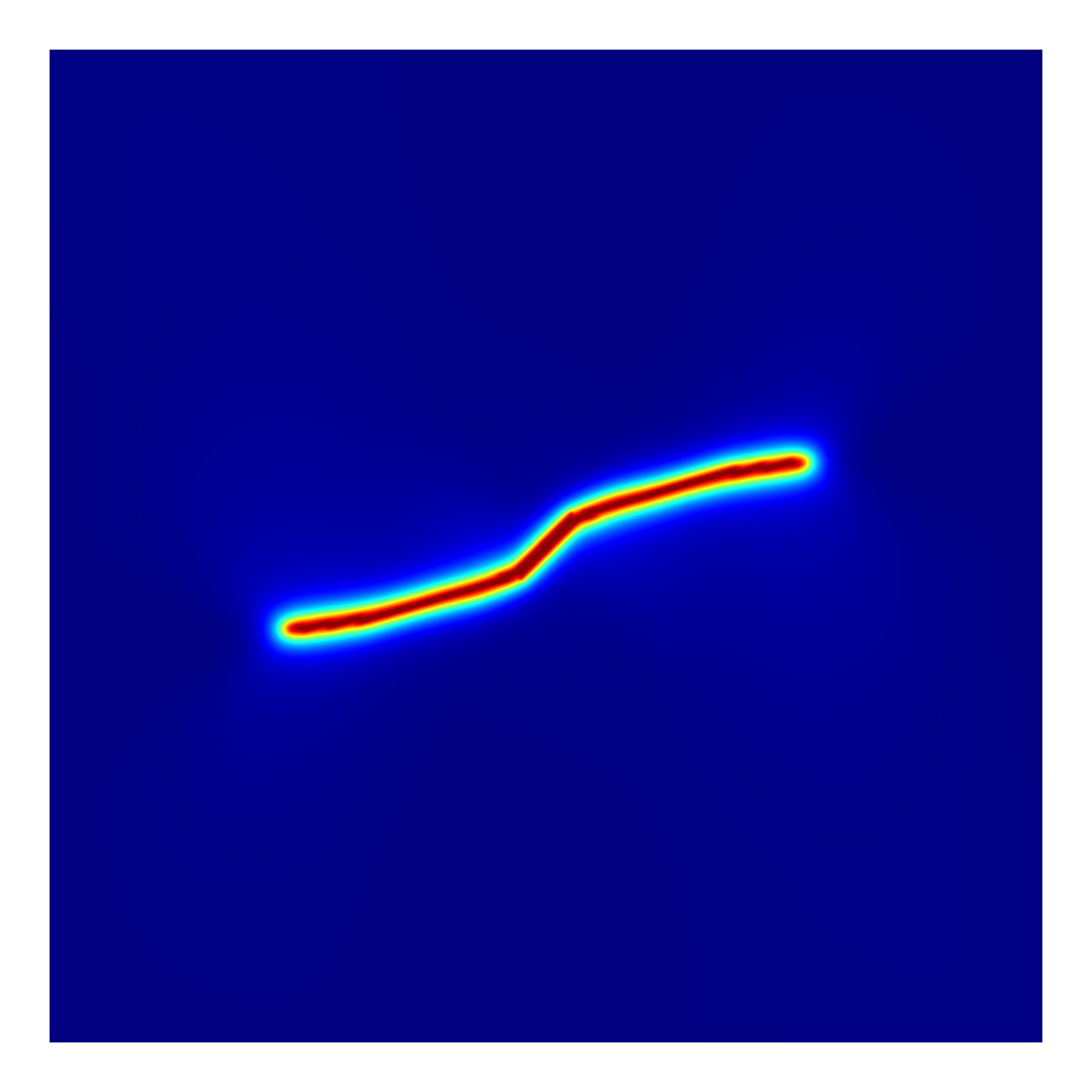
(c) $\sigma_{x0}/\sigma_{y0}=4$

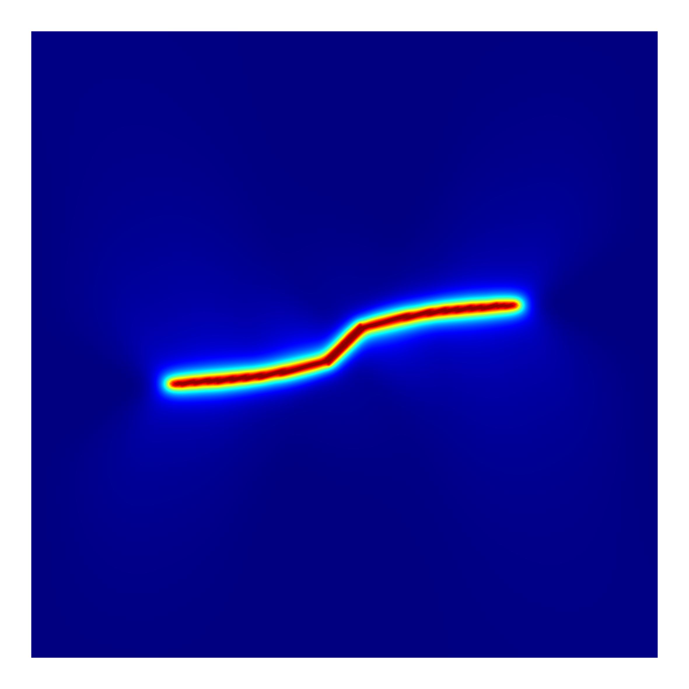
(d) $\sigma_{x0}/\sigma_{y0}=6$

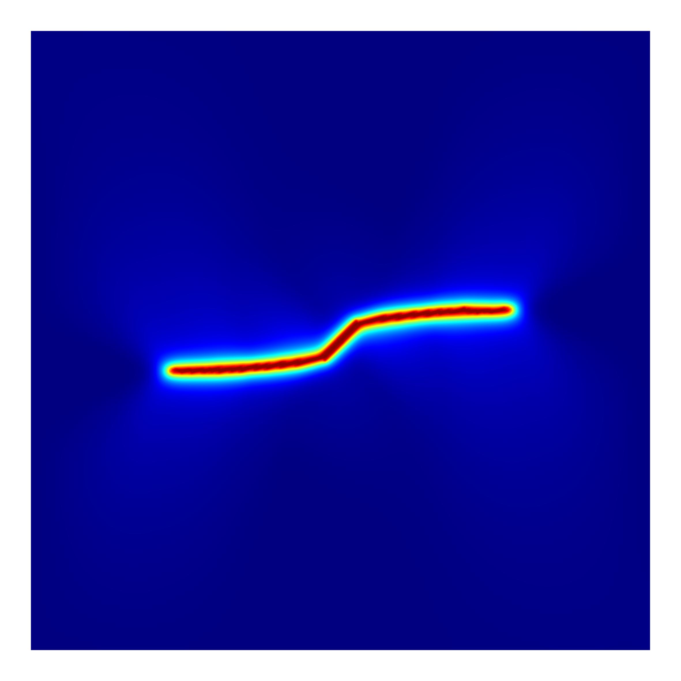
(e) $\sigma_{x0}/\sigma_{y0}=8$

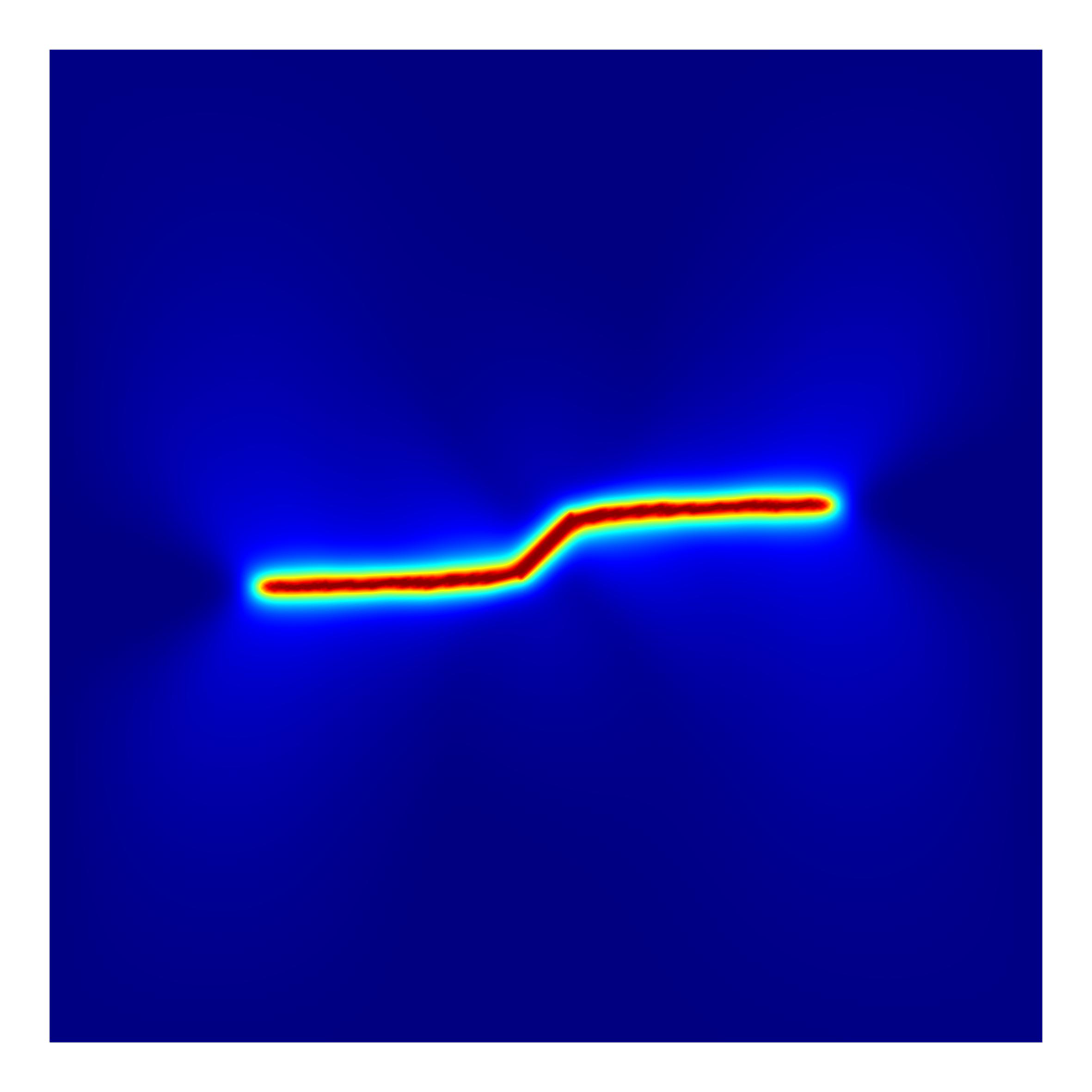
(f) $\sigma_{x0}/\sigma_{y0}=10$

Figure 14: Fracture propagation from an inclined initial notch at time $t=6$ s under different $\sigma_{x0}/\sigma_{y0}$

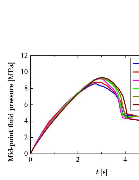
Figure 15: Effect of the ratio of $\sigma_{x0}/\sigma_{y0}$ on fluid pressure-time curve for an inclined initial notch

4.3 Fracture from two perpendicularly crossed notches

We also test the hydraulic fracture propagation from two perpendicularly crossed notches. The notches are located in the center of the calculation domain shown in Fig. 4 and both have a length of 0.8 m. The other simulation settings are the same as those in Subsection 4.1. We only consider four cases of in-situ stress as described in Table 3. This means that the direction of the maximum stress $S_{max}$ and the minimum stress $S_{min}$ varies in the four cases.

Table 3: Four cases of boundary and in-situ stresses

Case	Horizontal stress	Vertical stress
Case 1	$\sigma_{x0}=1$ MPa	$\sigma_{y0}=0.5$ MPa
Case 2	$\sigma_{x0}=5$ MPa	$\sigma_{y0}=0.5$ MPa
Case 3	$\sigma_{x0}=0.5$ MPa	$\sigma_{y0}=1$ MPa
Case 4	$\sigma_{x0}=0.5$ MPa	$\sigma_{y0}=5$ MPa

By using the proposed PFM, the phase field distribution for different cases is shown in Fig. 16. As observed, fractures only initiate and propagate from the notch perpendicular to the direction of the minimum stress $S_{min}$ while the other notches do not even grow. Note that the direction of these fractures is consistent with the direction of $S_{min}$. Therefore, Fig. 16 validates the engineering observation that the fractures perpendicular to the direction of the minimum in-situ stress will initiate and propagate more easily. The fluid pressure-time curves for different cases are shown in Fig. 17. The curves for Cases 1 and 3 and those for Case 2 and 4 are almost the same because the maximum and minimum in-situ stresses are identical.

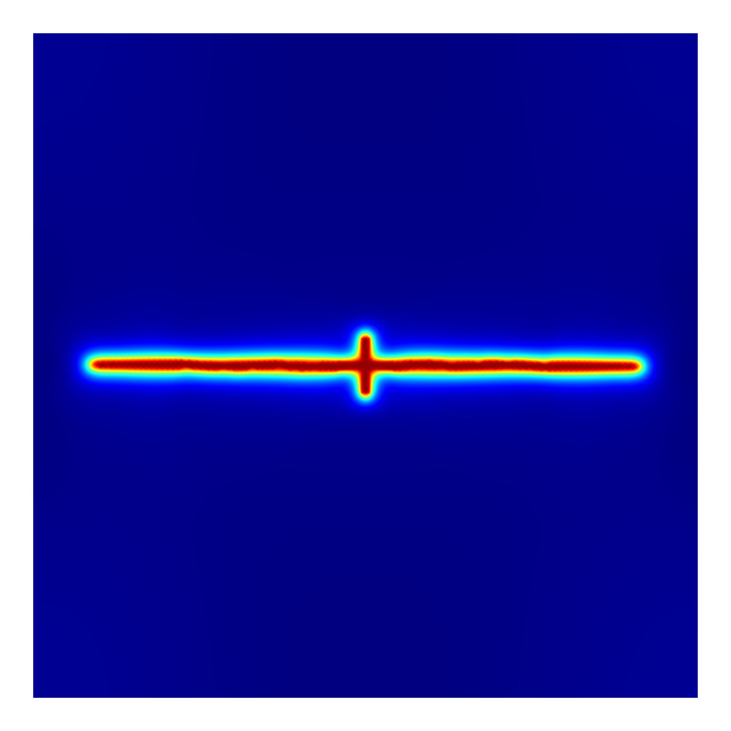
(a) Case 1

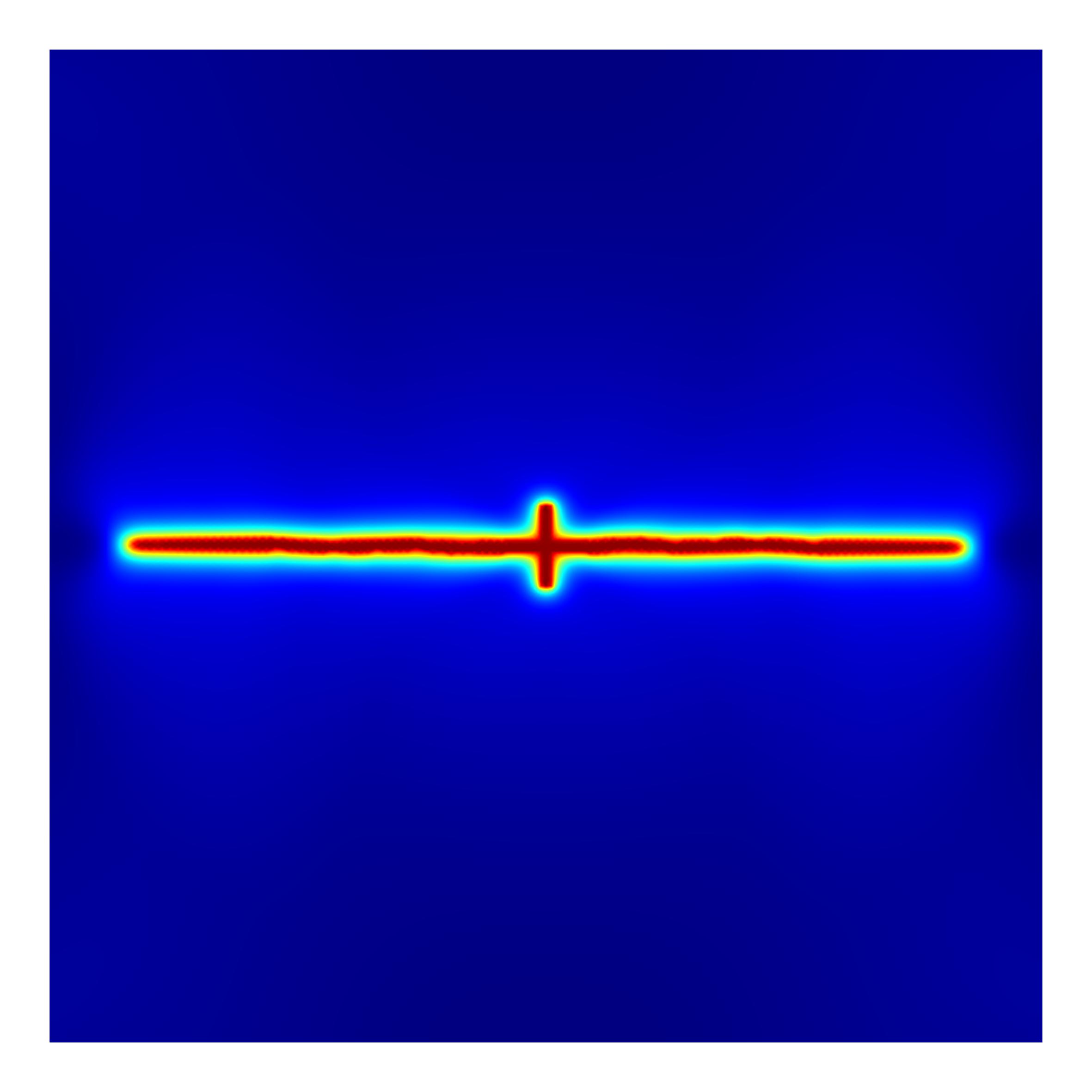
(b) Case 2

(c) Case 3

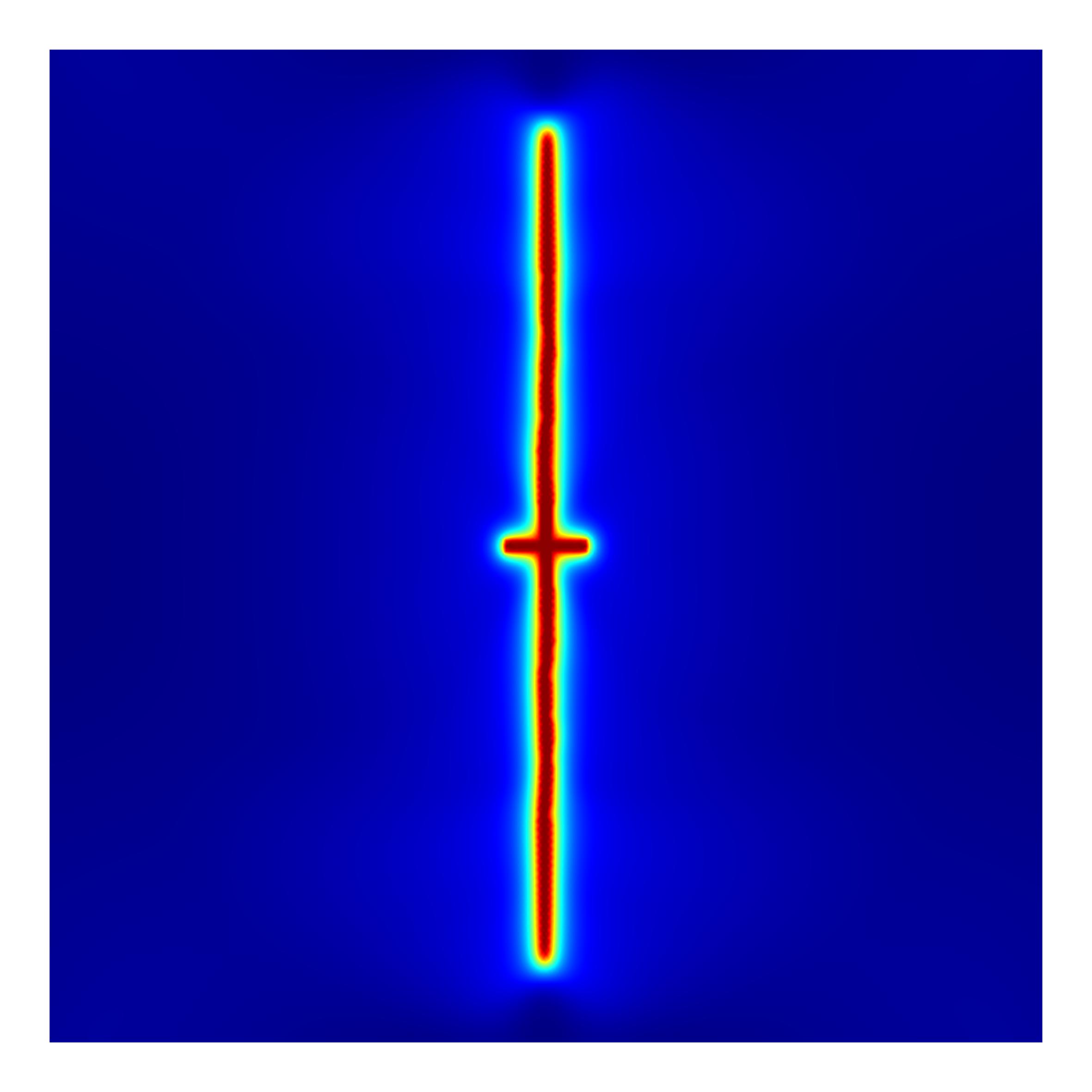
(d) Case 4

Figure 16: Fracture propagation from two perpendicularly crossed notches at time $t=5$ s

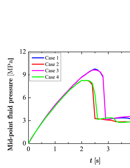
Figure 17: Fluid pressure-time curve for two perpendicularly crossed notch

4.4 Fracture from two horizontal notches

In this 2D example, hydraulic fracture from two horizontal notches is presented to further validate the proposed PFM. The geometry and boundary stress condition of this example are shown in Fig. 18a where the horizontal and vertical remote stresses are both 0.5 MPa for simplicity. The parameters and numerical settings are the same as Subsection 4.1. The phase field at $t=2.5$ s is shown in Fig. 18b. A symmetrical fracture pattern is observed and the fracture deflection occurs during fluid injection. This observation is in good agreement with the “stress shadowing” phenomenon in engineering practice [53].

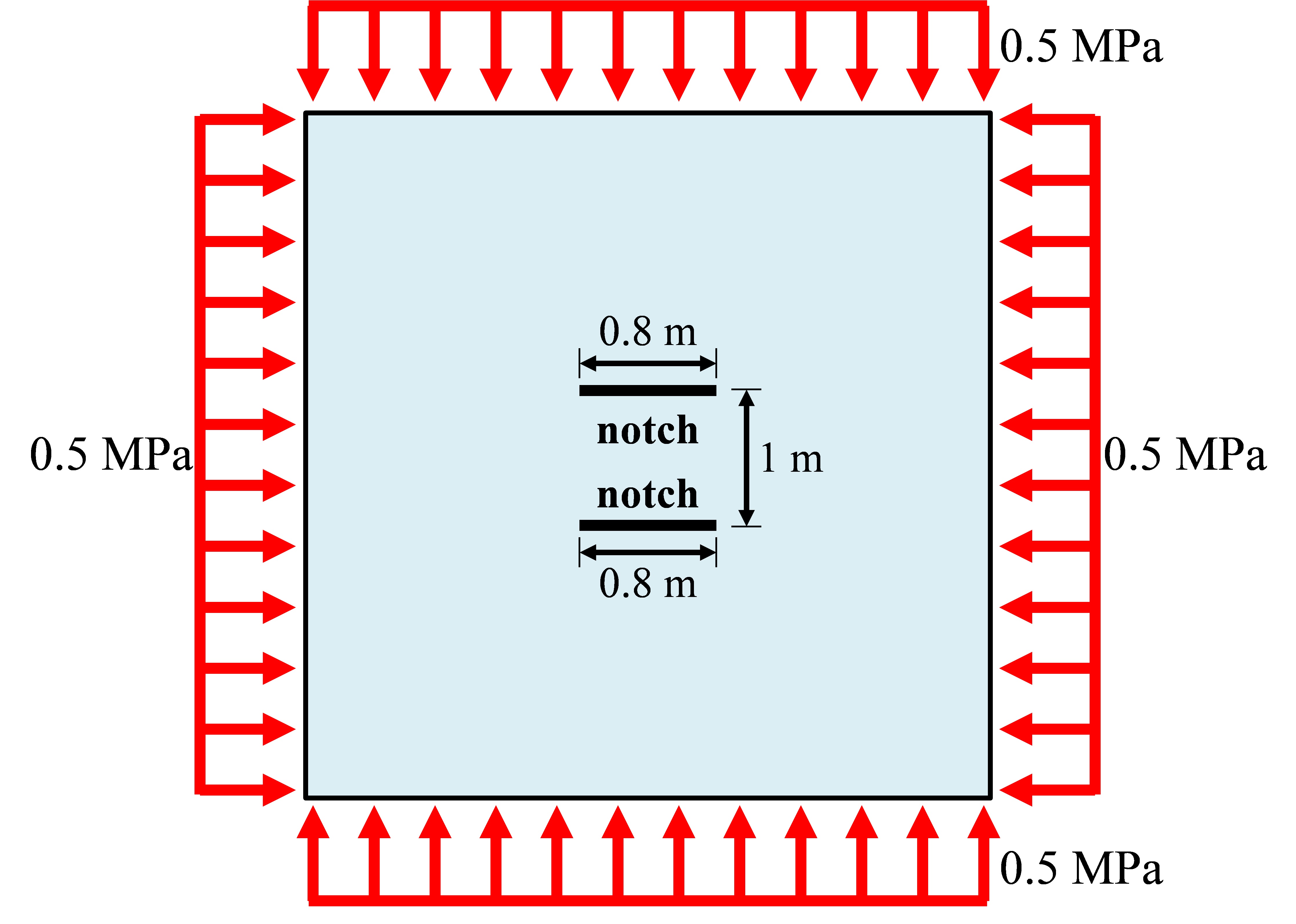
(a) Geometry and boundary condition

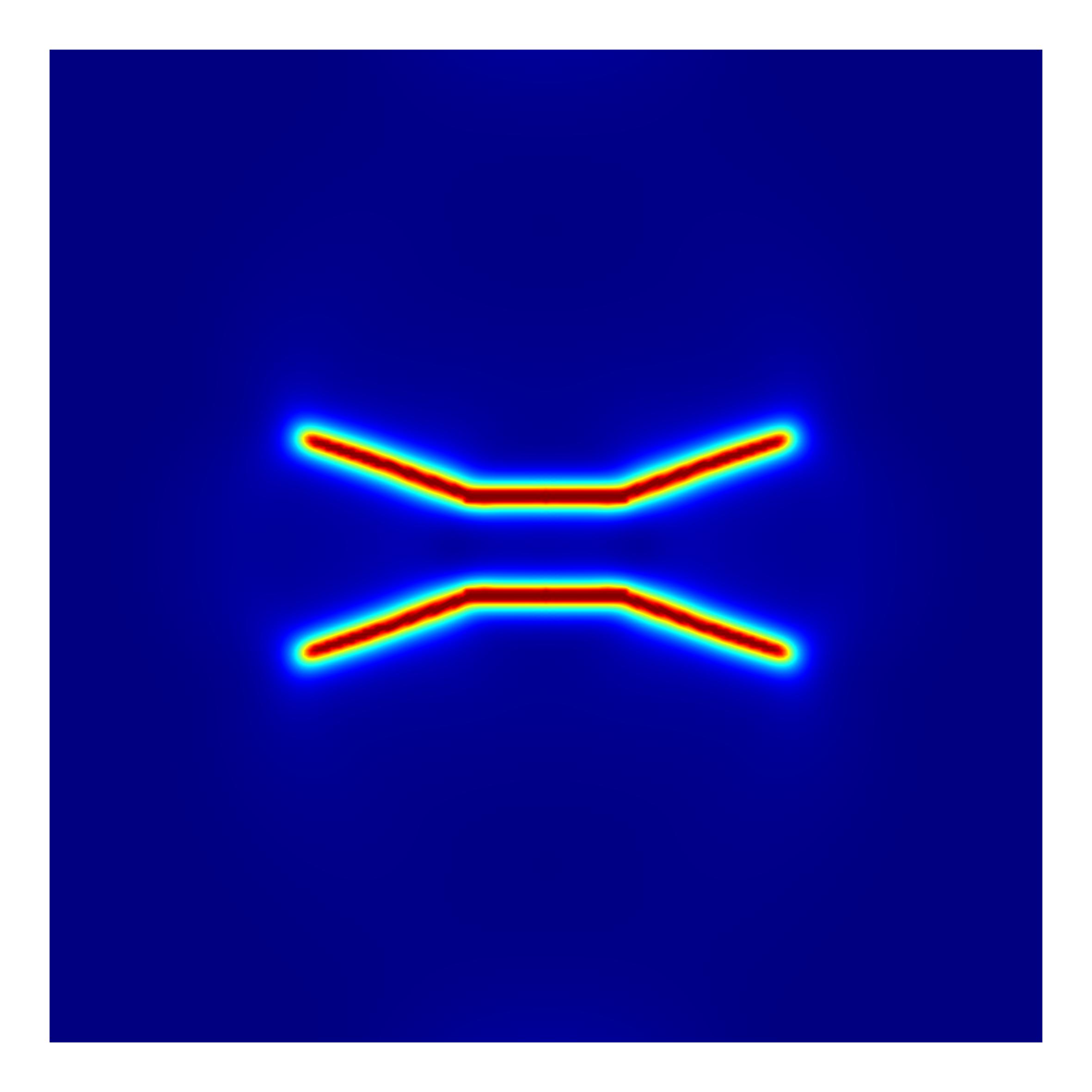
(b) Phase field at $t=2.5$ s

Figure 18: Fracture propagation from two horizontal notches

4.5 Linearly varying stress

In this final 2D example, we test the effect of linearly varying stress field on hydraulic fracture propagation. The geometry of this example is the same as that in Fig. 4 while the boundary stress condition is shown in 19. Note that in this example, the gravity is applied in the vertical direction, and linearly varying horizontal stress acts in the horizontal direction, which can be considered as a combination of self-weight stress field and tectonic stress field in underground geological environment. The parameters and numerical settings are the same as Subsection 4.1.

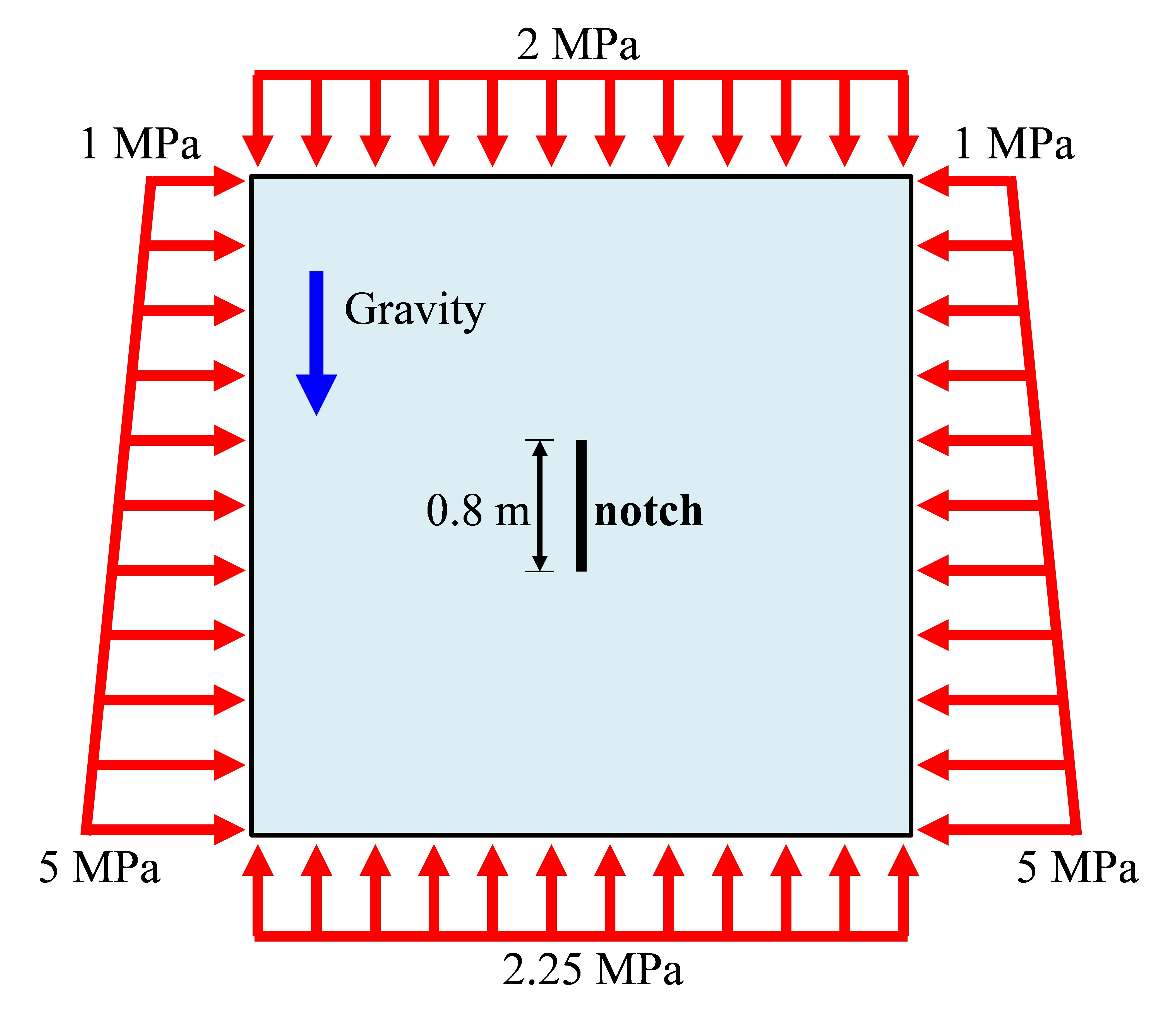
Figure 19: Linearly varying stress boundary condition

The phase field evolution at different time is shown in Fig. 20. An asymmetric fracture pattern is observed and the fracture propagation is much easier towards the upper boundary than towards the bottom. This finding can be also verified in Fig. 21, which depicts the fracture length increment at different time. Figure 21 indicates that the fracture length from the upper tip of the pre-existing notch is much larger than that from the lower tip. The downwards hydraulic fracture is hampered and even cannot propagate after $t=9$ s. Figures 20 and 21 strongly verifies that the hydraulic fracture tends to propagate towards the region with lowest fracture resistance.

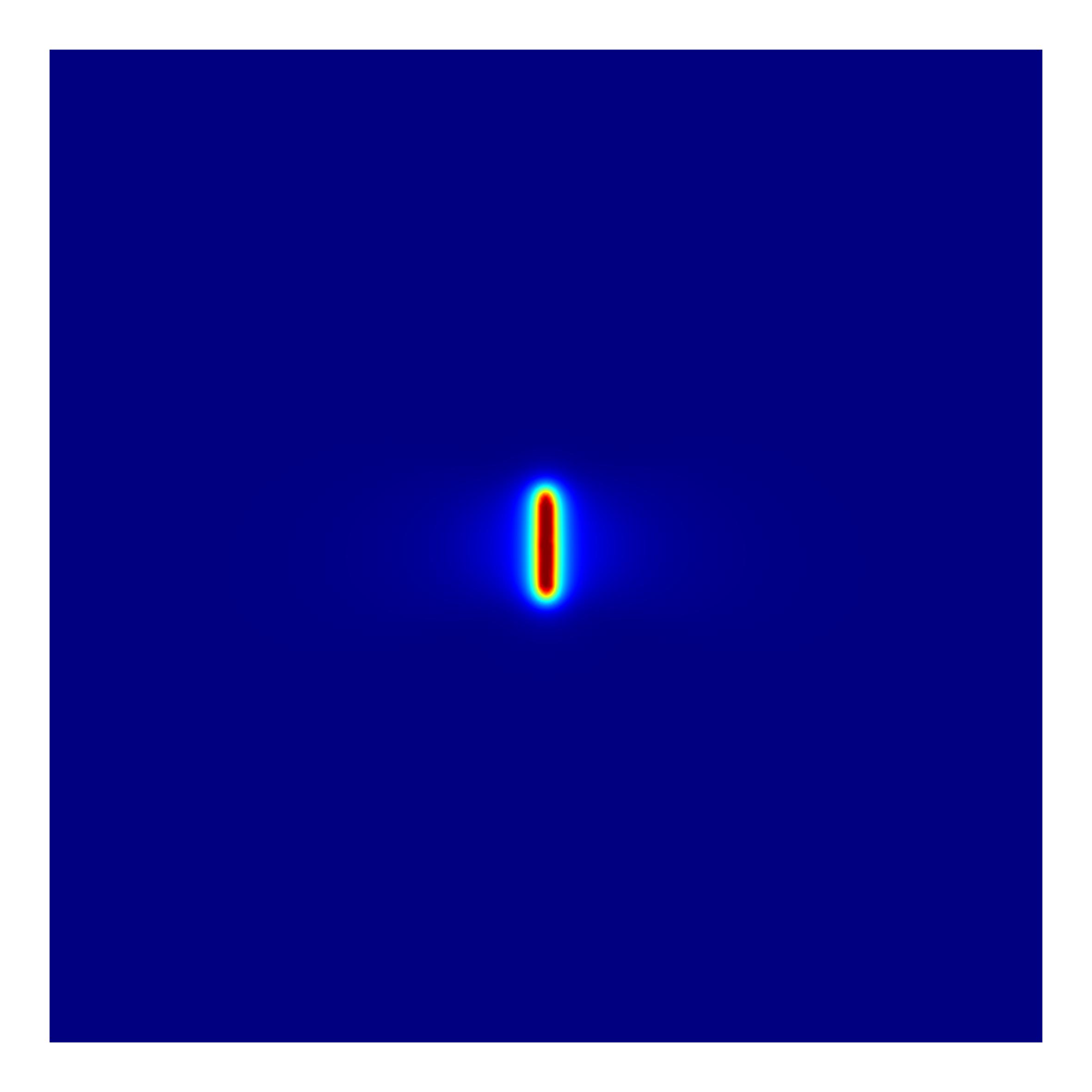
(a) $t=4$ s

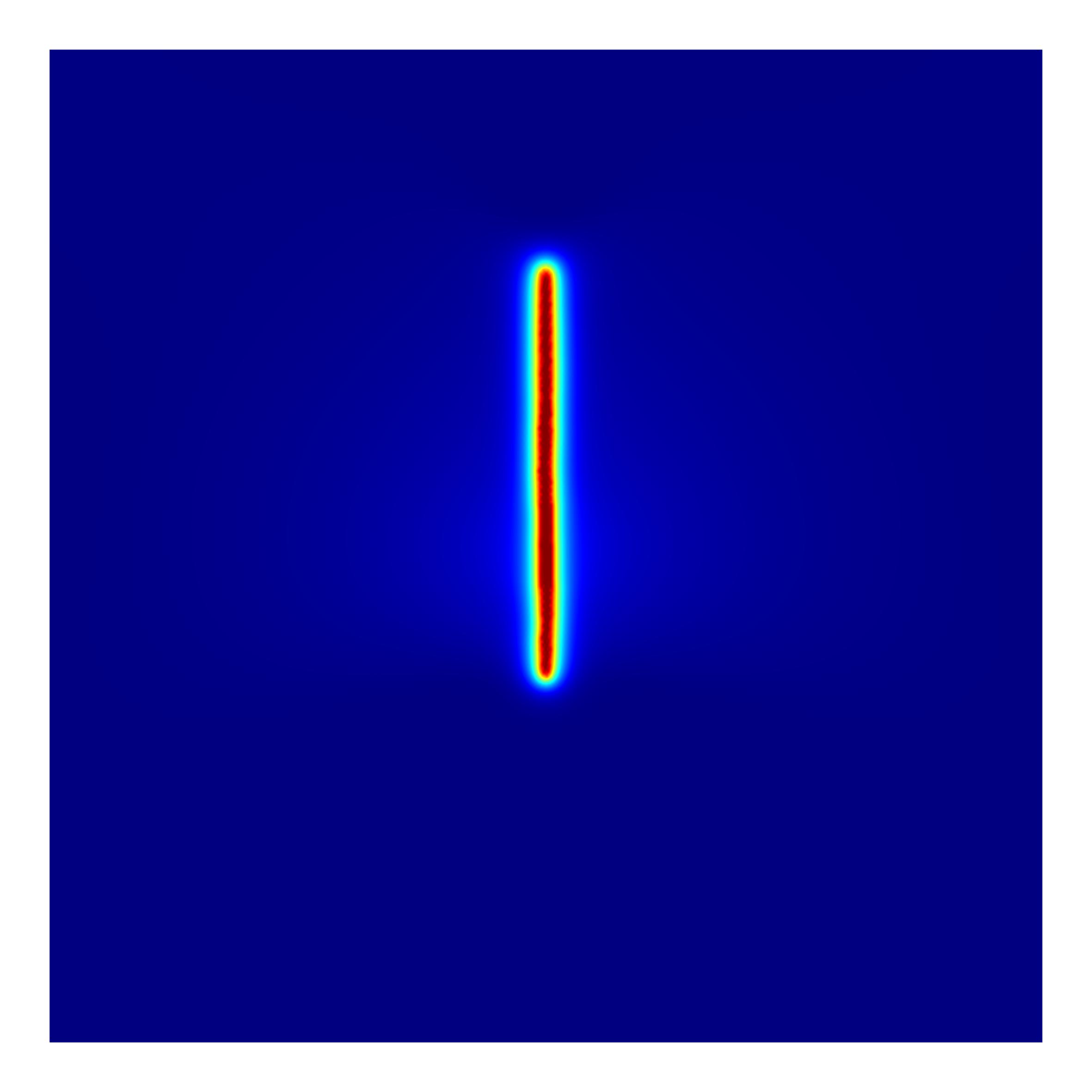
(b) $t=9$ s

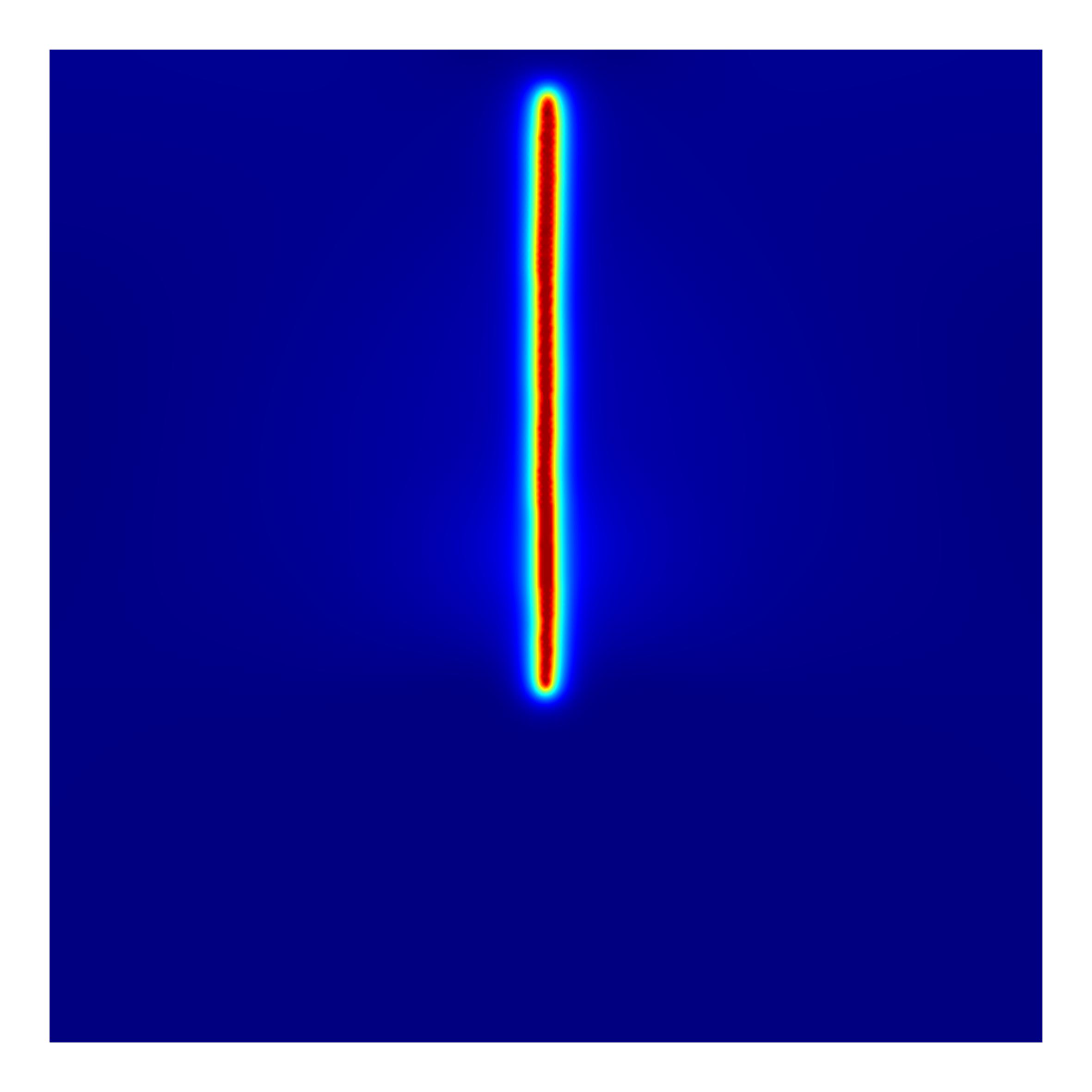
(c) $t=14$ s

Figure 20: Fracture propagation under varying vertical stress field

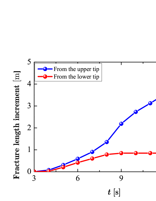
Figure 21: Fracture length increment under nearly varying stress field

In summary, the 2D examples in Subsections 4.1 to 4.5 indicate the sensitiveness of the hydraulic fracture propagation to the stress boundary condition. Our proposed model, which involves the effect of initial stress field, is feasible and practicable in capturing the effect of remote stresses on hydraulic fracture propagation and in producing the correct displacement field.

5 3D example

In this section, we test the performance of our method in modeling 3D hydraulic fracture propagation. Here, the last example is a 3D isotropic medium with a penny-shaped initial notch. The fluid source in the notch is set as $10$ kg/(m${}^{3}\cdot$s). The calculation domain is a cube with a dimension of $10\times 10\times 10$ m³ and has the same center as the initial notch, the height of which is in the $z$ direction. The notch is parallel to the $x$-$y$ plane and the radius and height are 0.8 m and 0.4 m, respectively.

The parameters for calculation are identical to those in Table 2 except the length scale parameter is $l_{0}=0.25$ m and the permeability $k_{f}$ is $5.21\times 10^{-3}$ m². We employ 6-node prism elements to discretize the 3D domain while the maximum element size is set as $0.18$ m for reducing computational cost. In addition, the time increment is set as 0.05 s in each simulation. In this 3D example, we only test the influence of the stress in the $z$ direction $\sigma_{z0}$. Therefore, $\sigma_{z0}$ is set as 0.5, 1, and 5 MPa, respectively, while the stresses in the other two directions are fixed to 1 MPa.

Hydraulic fracture propagation patterns in the 3D isotropic medium are shown in Fig. 22. It can be seen from Figs. 22a-f that for $\sigma_{z0}=0.5$ MPa and 1 MPa, the fractures initiate and propagate only in the $x$-$y$ plane while the area of the fractured domain increases as $\sigma_{z0}$ decreases. Figures 22g-i indicate that when $\sigma_{z0}$ is too large, the fracture propagation in the $x$-$y$ plane is hindered and fractures only propagate in the $x$-$z$ or $y$-$z$ plane.

The fluid pressure-time curves under different $\sigma_{z0}$ are shown in Fig. 23. The fluid pressure is observed to drop after fracture initiation and the maximum fluid pressure increases with the increase in the in-situ stress $\sigma_{z0}$. Comparing Figs. 22 and 23 indicate that the effect of in-situ stress on the 3D porous medium can be well captured by the proposed PFM in a fixed FE mesh without requiring any re-meshing or adaptive techniques. The 3D simulations fully verify the strong capability of our proposed PFM for predicting complex hydraulic fracture propagation in porous media subjected to stress boundary condition.

$\sigma_{z0}=0.5$ MPa
$\sigma_{z0}=1$ MPa
$\sigma_{z0}=5$ MPa

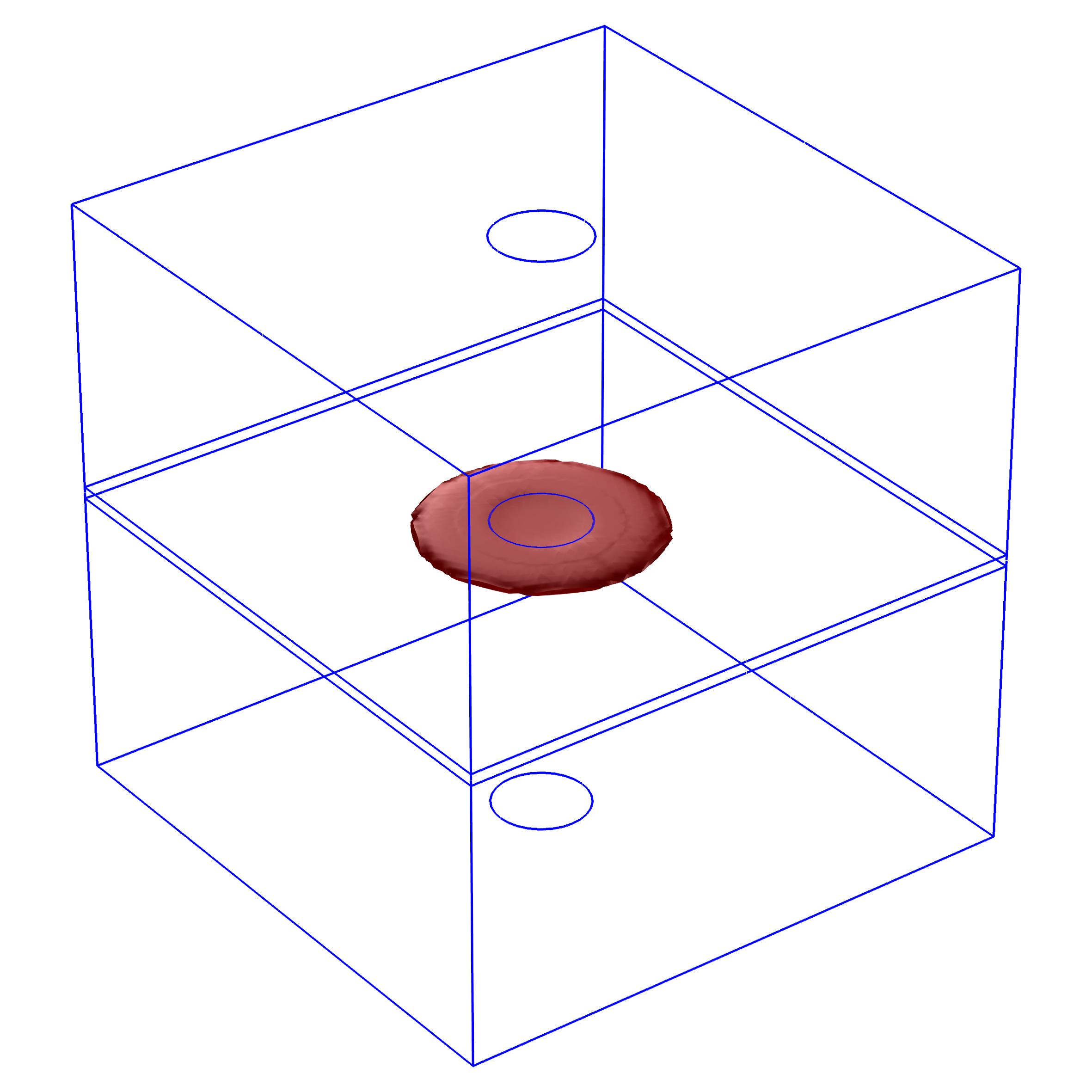
(a) $t=15$ s

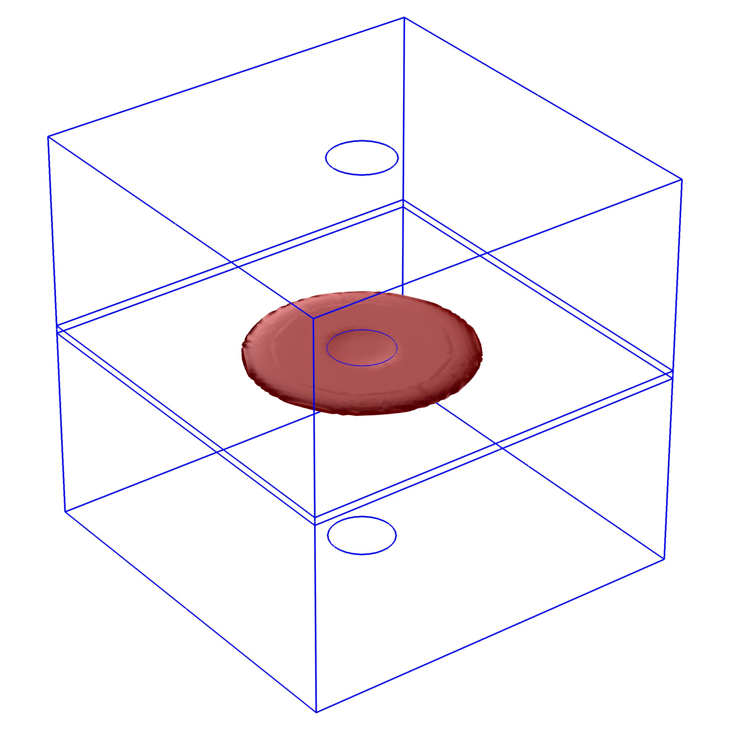
(b) $t=21$ s

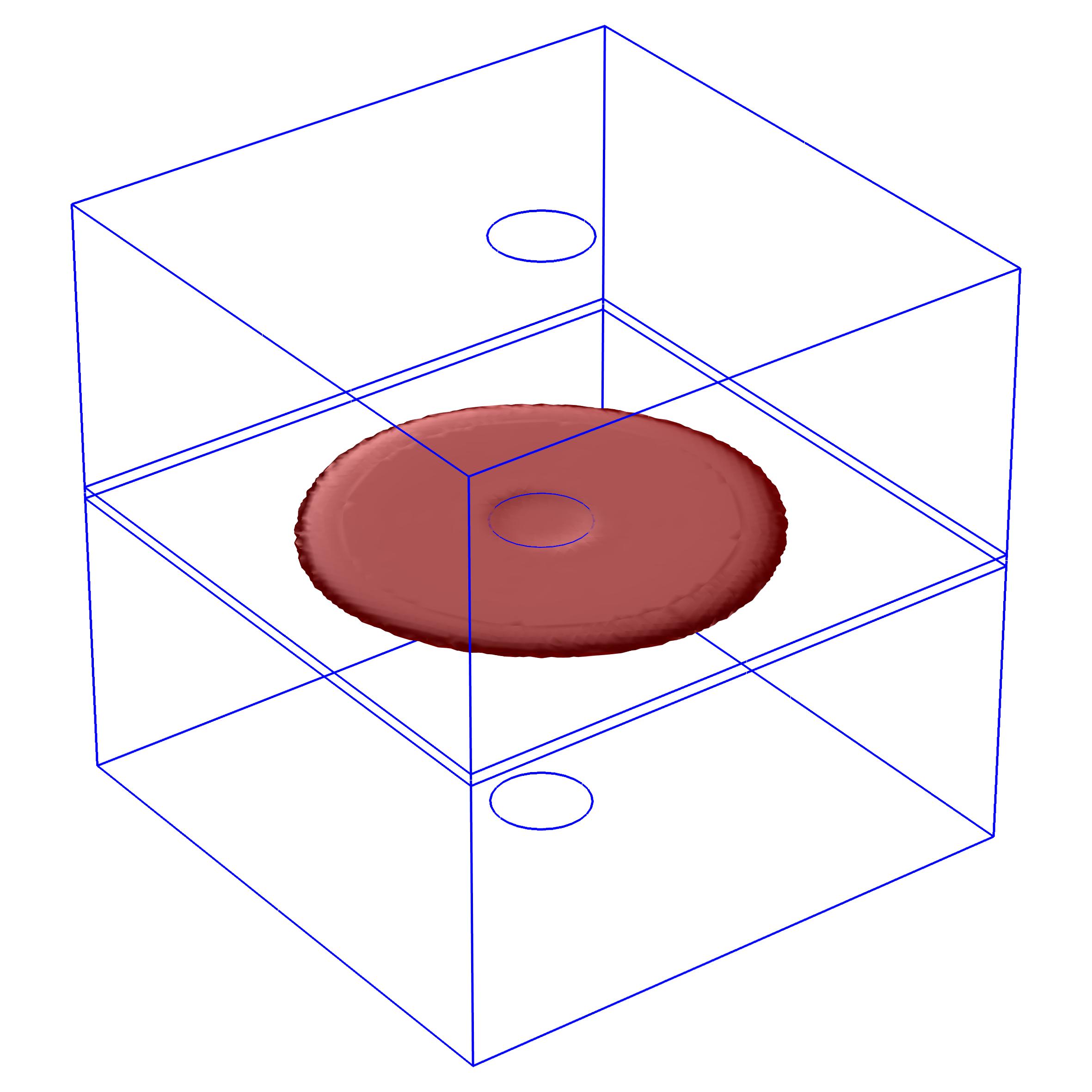
(c) $t=27$ s

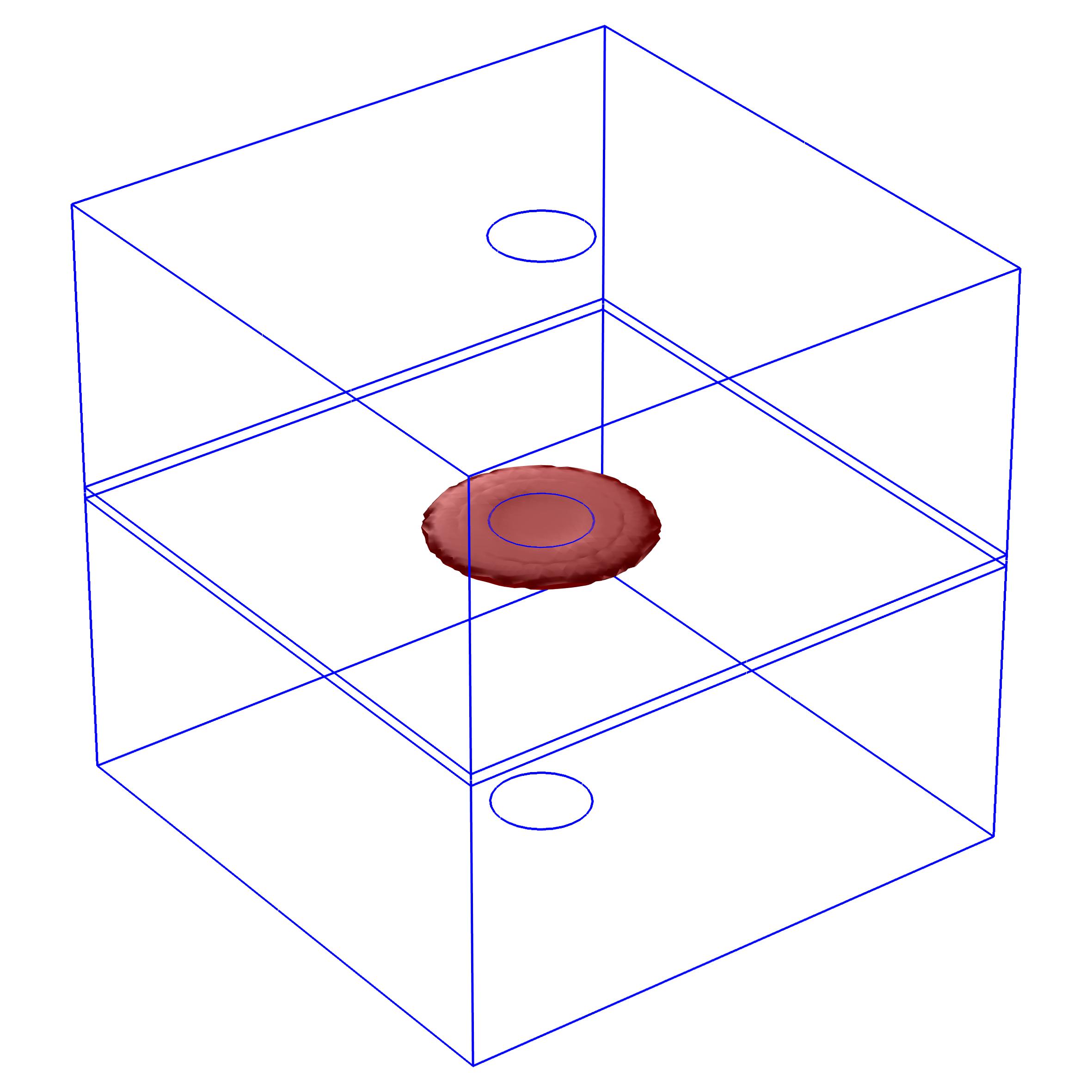
(d) $t=15$ s

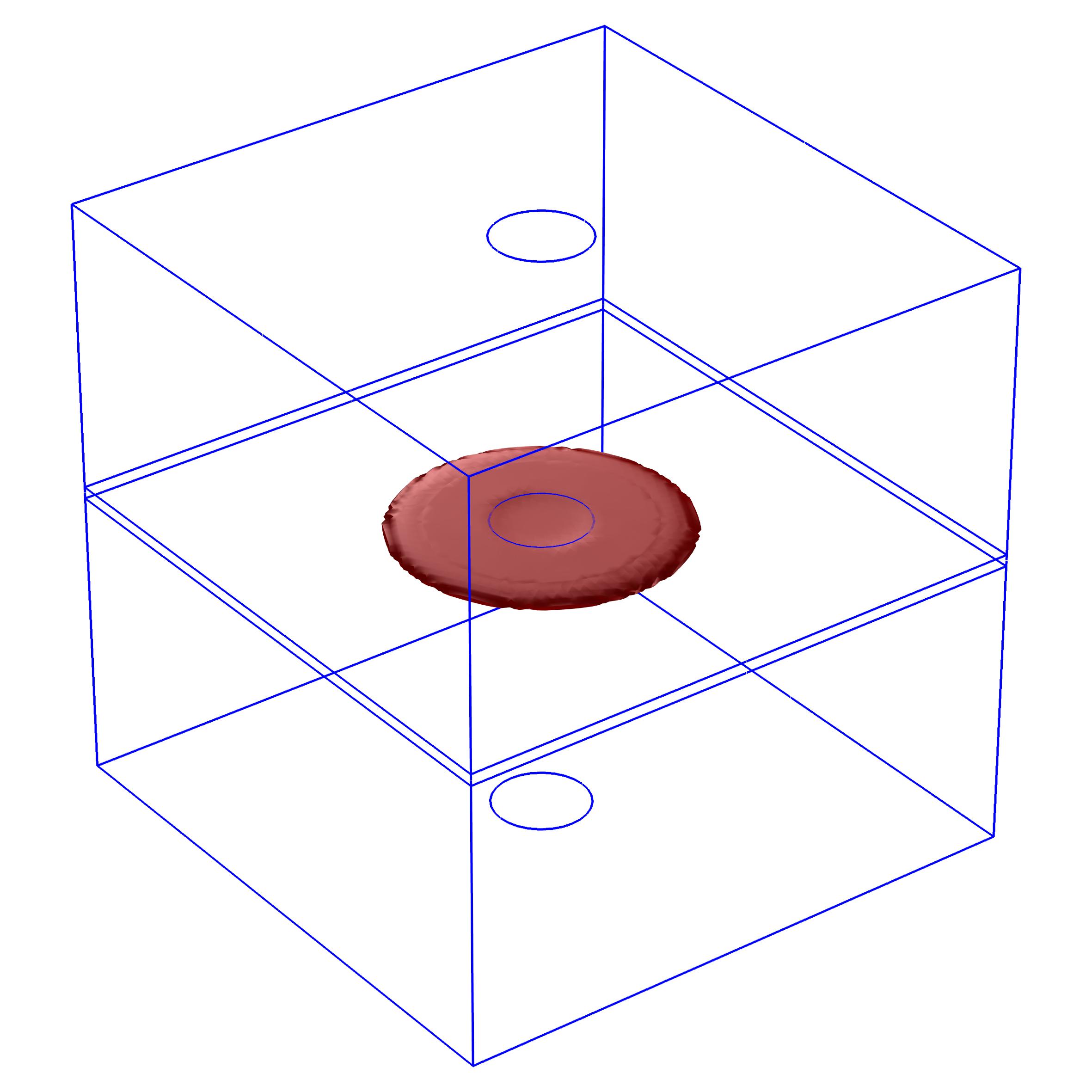
(e) $t=21$ s

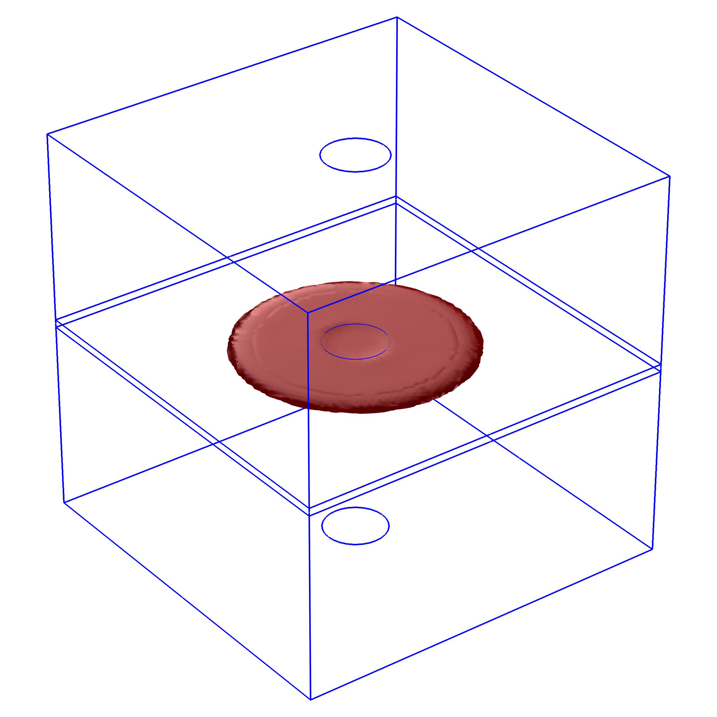
(f) $t=27$ s

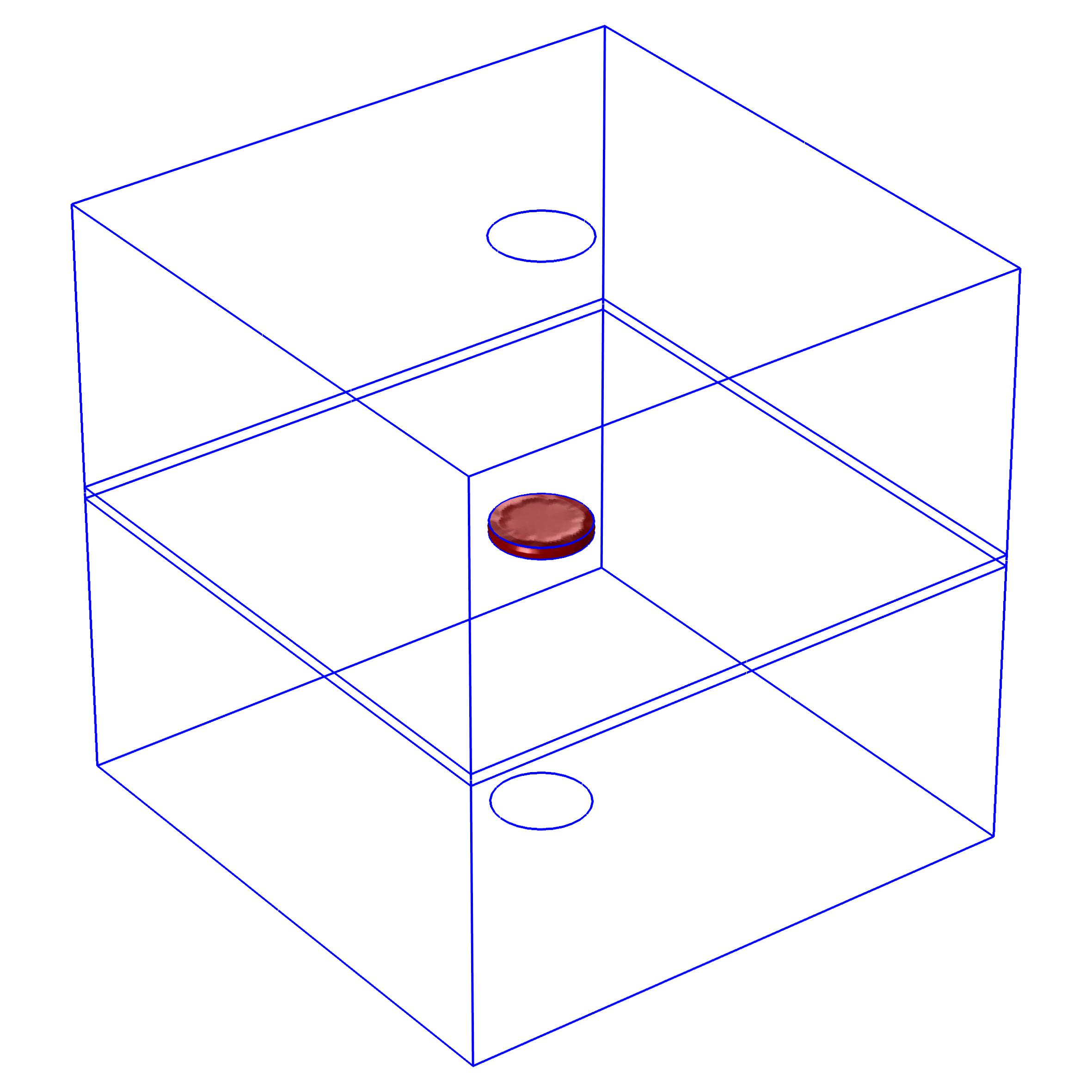
(g) $t=15$ s

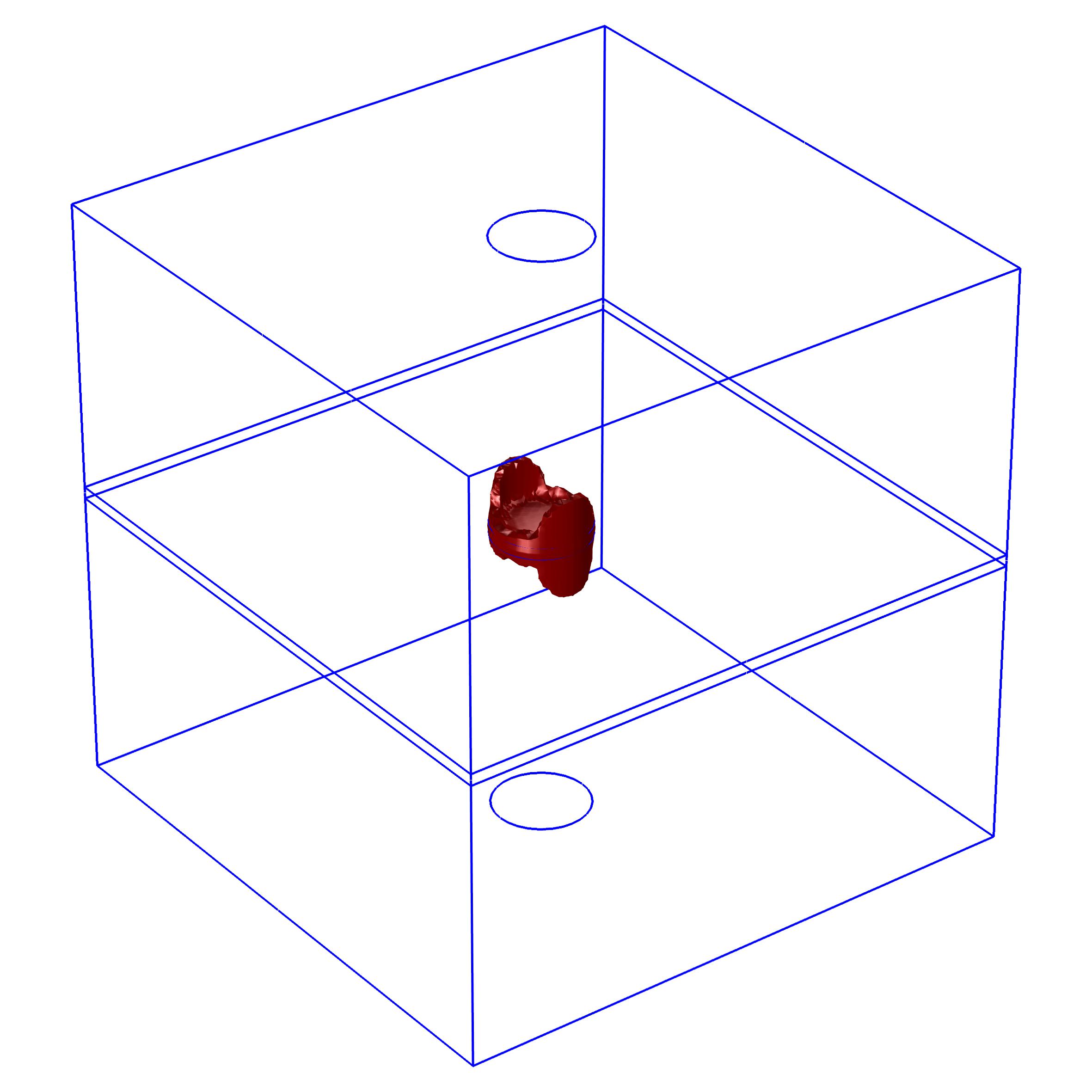
(h) $t=21$ s

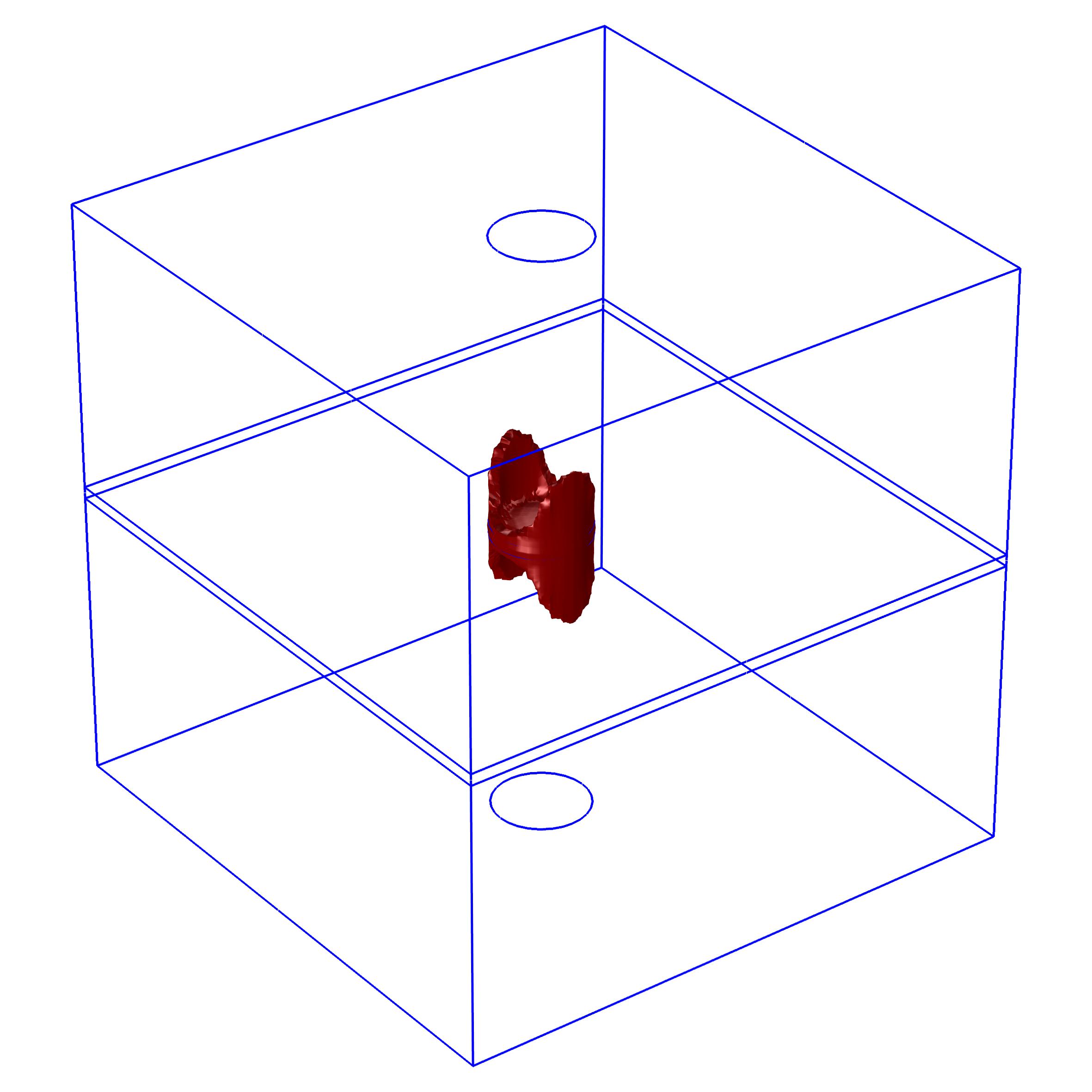
(i) $t=27$ s

Figure 22: Fracture evolution of the 3D isotropic porous medium with an interior notch under different $\sigma_{z0}$

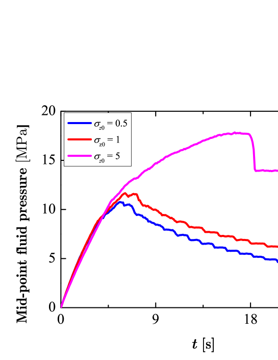
Figure 23: Fluid pressure-time curve for 3D porous medium

6 Conclusions

A new phase field model for simulating quasi-static hydraulic fracture propagation in porous media subjected to stress boundary conditions is proposed. A new energy functional is established to consider the effect of initial in-situ stress field. This energy functional is then used to achieve the governing equations for the displacement and phase fields through the variational approach. Biot poroelasticity theory is used to couple the fluid pressure field and the displacement field while the phase field is used for determining the fluid properties from the intact domain to the fully broken domain.

The presented numerical examples in this work verify the capability of the proposed PFM in capturing complex hydraulic fracture growth patterns in 2D and 3D. The numerical examples also indicate that under stress boundary conditions the proposed approach can obtain correct displacement distribution and reflect the sensitiveness of hydraulic fracture propagation to stress boundary conditions. In future research, the proposed PFM can be more widely applied in HF practices where the stress boundaries are dominated and can be used to investigate the influence of naturally-layered porous media and multi-zone HF on fracture propagation.

Appendix Finite element discretization

We first derive the weak forms of all the governing equations as

$$\int_{\Omega}\left[(\bm{\sigma}^{e}+g(\phi)\bm{\sigma}_{0}-\alpha p\bm{I}):\delta\bm{\varepsilon}\right]\mathrm{d}\Omega=\int_{\Omega_{h}}\bm{f}_{t}\cdot\delta\bm{u}\mathrm{d}S$$ (29)

$$\int_{\Omega}-2(1-k)H(1-\phi)\delta\phi\mathrm{d}\Omega+\int_{\Omega}G_{c}\left(l_{0}\nabla\phi\cdot\nabla\delta\phi+\frac{1}{l_{0}}\phi\delta\phi\right)\mathrm{d}\Omega=0$$ (30)

$$\int_{\Omega}\rho S\frac{\partial p}{\partial t}\delta p\mathrm{d}\Omega-\int_{\Omega}\rho\bm{v}\cdot\nabla\delta p\mathrm{d}\Omega=\int_{\partial\Omega_{N}}M_{n}\mathrm{d}S+\int_{\Omega}\left(q_{m}-\rho\alpha\chi_{R}\frac{\partial\varepsilon_{vol}}{\partial t}\right)\mathrm{d}\Omega$$ (31)

In an element with $n$ nodes, the nodal values for the three fields ($\bm{u}$, $\phi$, and $p$) are defined as $\bm{u}_{i}$, $\phi_{i}$, and $p_{i}$ ($i=1,2,\cdots,n$). The fields are then discretized as follows,

$$\bm{u}=\sum_{i}^{n}N_{i}\bm{u}_{i},\hskip 14.22636pt\phi=\sum_{i}^{n}N_{i}\phi_{i},\hskip 14.22636ptp=\sum_{i}^{n}N_{i}p_{i}$$ (32)

where $N_{i}$ is the shape function at node $i$. We then derive the gradients of the three fields as

$$\bm{\varepsilon}=\sum_{i}^{n}\mathbf{B}_{i}^{u}\bm{u}_{i},\hskip 14.22636pt\nabla\phi=\sum_{i}^{n}\mathbf{B}_{i}^{\phi}\phi_{i},\hskip 14.22636pt\nabla p=\sum_{i}^{n}\mathbf{B}_{i}^{p}p_{i}$$ (33)

where $\mathbf{B}_{i}^{u}$, $\mathbf{B}_{i}^{\phi}$, and $\mathbf{B}_{i}^{p}$ are derivatives of the shape functions:

$$\mathbf{B}_{i}^{u}=\left[\begin{array}[]{cccccc}N_{i,x}&0&0&N_{i,y}&0&N_{i,z}\\ 0&N_{i,y}&0&N_{i,x}&N_{i,z}&0\\ 0&0&N_{i,z}&0&N_{i,y}&N_{i,x}\\ \end{array}\right]^{\mathrm{T}},\hskip 14.22636pt\mathbf{B}_{i}^{\phi}=\mathbf{B}_{i}^{p}=\left[\begin{array}[]{ccc}N_{i,x}\\ N_{i,y}\\ N_{i,z}\end{array}\right]$$ (34)

For 2D, the components along the $z$ direction is removed from above equations (34). Due to the arbitrariness in the test functions, the external force $\mathbf{F}_{i}^{u,ext}$ and inner force $\mathbf{F}_{i}^{u,int}$ for the displacement field are described by

$$\left\{\begin{aligned} \mathbf{F}_{i}^{u,ext}&=\int_{\Omega_{h}}N_{i}\bm{f}_{t}\mathrm{d}S+\int_{\Omega}[\mathbf{B}_{i}^{u}]^{\mathrm{T}}\alpha p\bm{I}\mathrm{d}\Omega-\int_{\Omega}[\mathbf{B}_{i}^{u}]^{\mathrm{T}}g(\phi)\bm{\sigma}_{0}\mathrm{d}\Omega\\ \mathbf{F}_{i}^{u,int}&=\int_{\Omega}[\mathbf{B}_{i}^{u}]^{\mathrm{T}}\bm{\sigma}\mathrm{d}\Omega\end{aligned}\right.$$ (35)

The inner force term of the phase field is also obtained by

$$F_{i}^{\phi,int}=\int_{\Omega}-2(1-k)(1-\phi)HN_{i}+G_{c}\left(l_{0}[\mathbf{B}_{i}^{\phi}]^{\mathrm{T}}\nabla\phi+\frac{1}{l_{0}}\phi N_{i}\right)\mathrm{d}\Omega$$ (36)

Finally, for the pressure field, the inner force $F_{i}^{p,int}$, viscous force $F_{i}^{p,vis}$, and external force $F_{i}^{p,ext}$ are given by

$$\left\{\begin{aligned} F_{i}^{p,int}&=\int_{\Omega}[\mathbf{B}_{i}^{p}]^{\mathrm{T}}\frac{\rho K_{eff}}{\mu_{eff}}\nabla p\mathrm{d}\Omega\\ F_{i}^{p,vis}&=\int_{\Omega}N_{i}\rho S\frac{\partial p}{\partial t}\mathrm{d}\Omega\\ F_{i}^{p,ext}&=\int_{\Omega}N_{i}\left(q_{m}-\rho\alpha\chi_{R}\frac{\partial\varepsilon_{vol}}{\partial t}\right)\mathrm{d}\Omega+\int_{\partial\Omega_{N}}N_{i}M_{N}\mathrm{d}S\end{aligned}\right.$$ (37)

Thus, contribution of node $i$ to the residual of the discrete equations for the three field is written as

$$\left\{\begin{aligned} \mathbf{R}_{i}^{u}&=\mathbf{F}_{i}^{u,ext}-\mathbf{F}_{i}^{u,int}\\ R_{i}^{\phi}&=-F_{i}^{\phi,int}\\ R_{i}^{p}&=F_{i}^{p,ext}-F_{i}^{p,int}-F_{i}^{p,vis}\end{aligned}\right.$$ (38)

Because the staggered scheme is used to solve the displacement, phase field and fluid pressure sequentially. We also adopt the Newton-Raphson approach sequentially to achieve $\mathbf{R}_{i}^{u}=\bm{0}$, $R_{i}^{\phi}=0$, and $R_{i}^{p}=0$ for the three fields. In addition, the tangents on the element level are calculated by

$$\left\{\begin{aligned} \mathbf{K}_{ij}^{uu}&=\frac{\partial\mathbf{F}_{i}^{u,int}}{\partial\bm{u}_{j}}=\int_{\Omega}[\mathbf{B}_{i}^{u}]^{\mathrm{T}}\mathbf{D}_{e}[\mathbf{B}_{j}^{u}]\mathrm{d}\Omega\\ \mathbf{K}_{ij}^{\phi\phi}&=\frac{\partial F_{i}^{\phi,int}}{\partial\phi_{j}}=\int_{\Omega}\left\{[\mathbf{B}_{i}^{\phi}]^{\mathrm{T}}G_{c}l_{0}[\mathbf{B}_{j}^{\phi}]+N_{i}\left(2(1-k)H+\frac{G_{c}}{l_{0}}\right)N_{j}\right\}\mathrm{d}\Omega\\ \mathbf{K}_{ij}^{pp}&=\frac{\partial F_{i}^{p,int}}{\partial p_{j}}=\int_{\Omega}[\mathbf{B}_{i}^{p}]^{\mathrm{T}}\frac{\rho K_{eff}}{\mu_{eff}}[\mathbf{B}_{j}^{p}]\mathrm{d}\Omega\end{aligned}\right.$$ (39)

where $\mathbf{D}_{e}$ is the elasticity matrices derived from the elasticity tensor $\bm{D}={\partial\bm{\sigma}^{e}}/{\partial\bm{\varepsilon}}$.

References

- Settari et al. [1980] A. Settari, et al., Simulation of hydraulic fracturing processes, Society of Petroleum Engineers Journal 20 (06) (1980) 487–500.
- Bredehoeft et al. [1976] J. Bredehoeft, R. Wolff, W. Keys, E. Shuter, Hydraulic fracturing to determine the regional in situ stress field, Piceance Basin, Colorado, Geological Society of America Bulletin 87 (2) (1976) 250–258.
- Häring et al. [2008] M. O. Häring, U. Schanz, F. Ladner, B. C. Dyer, Characterisation of the Basel 1 enhanced geothermal system, Geothermics 37 (5) (2008) 469–495.
- Osborn et al. [2011] S. G. Osborn, A. Vengosh, N. R. Warner, R. B. Jackson, Methane contamination of drinking water accompanying gas-well drilling and hydraulic fracturing, Proceedings of the National Academy of Sciences 108 (20) (2011) 8172–8176.
- Vidic et al. [2013] R. D. Vidic, S. L. Brantley, J. M. Vandenbossche, D. Yoxtheimer, J. D. Abad, Impact of shale gas development on regional water quality, Science 340 (6134) (2013) 1235009.
- Moës and Belytschko [2002] N. Moës, T. Belytschko, Extended finite element method for cohesive crack growth, Engineering fracture mechanics 69 (7) (2002) 813–833.
- Chen et al. [2012] L. Chen, T. Rabczuk, S. P. A. Bordas, G. Liu, K. Zeng, P. Kerfriden, Extended finite element method with edge-based strain smoothing (ESm-XFEM) for linear elastic crack growth, Computer Methods in Applied Mechanics and Engineering 209 (2012) 250–265.
- Fries and Belytschko [2010] T.-P. Fries, T. Belytschko, The extended/generalized finite element method: an overview of the method and its applications, International Journal for Numerical Methods in Engineering 84 (3) (2010) 253–304.
- Fu et al. [2013] Z.-J. Fu, W. Chen, H.-T. Yang, Boundary particle method for Laplace transformed time fractional diffusion equations, Journal of Computational Physics 235 (2013) 52–66.
- Fu et al. [2018a] Z. Fu, W. Chen, P. Wen, C. Zhang, Singular boundary method for wave propagation analysis in periodic structures, Journal of Sound and Vibration 425 (2018a) 170–188.
- Fu et al. [2018b] Z.-J. Fu, Q. Xi, W. Chen, A. H.-D. Cheng, A boundary-type meshless solver for transient heat conduction analysis of slender functionally graded materials with exponential variations, Computers & Mathematics with Applications .
- Chau-Dinh et al. [2012] T. Chau-Dinh, G. Zi, P.-S. Lee, T. Rabczuk, J.-H. Song, Phantom-node method for shell models with arbitrary cracks, Computers & Structures 92 (2012) 242–256.
- Rabczuk et al. [2008] T. Rabczuk, G. Zi, A. Gerstenberger, W. A. Wall, A new crack tip element for the phantom-node method with arbitrary cohesive cracks, International Journal for Numerical Methods in Engineering 75 (5) (2008) 577–599.
- Belytschko and Lin [1987] T. Belytschko, J. I. Lin, A three-dimensional impact-penetration algorithm with erosion, International Journal of Impact Engineering 5 (1-4) (1987) 111–127.
- Johnson and Stryk [1987] G. R. Johnson, R. A. Stryk, Eroding interface and improved tetrahedral element algorithms for high-velocity impact computations in three dimensions, International Journal of Impact Engineering 5 (1-4) (1987) 411–421.
- Peerlings et al. [1996] R. Peerlings, R. De Borst, W. Brekelmans, J. De Vree, I. Spee, Some observations on localisation in non-local and gradient damage models, European Journal of Mechanics A: Solids 15 (6) (1996) 937–953.
- Areias et al. [2016] P. Areias, M. Msekh, T. Rabczuk, Damage and fracture algorithm using the screened Poisson equation and local remeshing, Engineering Fracture Mechanics 158 (2016) 116–143.
- Bourdin et al. [2008] B. Bourdin, G. A. Francfort, J.-J. Marigo, The variational approach to fracture, Journal of elasticity 91 (1) (2008) 5–148.
- Miehe et al. [2010a] C. Miehe, F. Welschinger, M. Hofacker, Thermodynamically consistent phase-field models of fracture: Variational principles and multi-field FE implementations, International Journal for Numerical Methods in Engineering 83 (10) (2010a) 1273–1311.
- Miehe et al. [2010b] C. Miehe, M. Hofacker, F. Welschinger, A phase field model for rate-independent crack propagation: Robust algorithmic implementation based on operator splits, Computer Methods in Applied Mechanics and Engineering 199 (45) (2010b) 2765–2778.
- Zhou et al. [2018a] S. Zhou, X. Zhuang, H. Zhu, T. Rabczuk, Phase field modelling of crack propagation, branching and coalescence in rocks, Theoretical and Applied Fracture Mechanics 96 (2018a) 174–192.
- Zhou et al. [2019a] S. Zhou, X. Zhuang, T. Rabczuk, Phase field modeling of brittle compressive-shear fractures in rock-like materials: A new driving force and a hybrid formulation, Computer Methods in Applied Mechanics and Engineering 355 (2019a) 729–752.
- Ambati et al. [2015] M. Ambati, T. Gerasimov, L. De Lorenzis, A review on phase-field models of brittle fracture and a new fast hybrid formulation, Computational Mechanics 55 (2) (2015) 383–405.
- Borden et al. [2012] M. J. Borden, C. V. Verhoosel, M. A. Scott, T. J. Hughes, C. M. Landis, A phase-field description of dynamic brittle fracture, Computer Methods in Applied Mechanics and Engineering 217 (2012) 77–95.
- Hofacker and Miehe [2012] M. Hofacker, C. Miehe, Continuum phase field modeling of dynamic fracture: variational principles and staggered FE implementation, International Journal of Fracture (2012) 1–17.
- Hofacker and Miehe [2013] M. Hofacker, C. Miehe, A phase field model of dynamic fracture: Robust field updates for the analysis of complex crack patterns, International Journal for Numerical Methods in Engineering 93 (3) (2013) 276–301.
- Khatir and Wahab [2019a] S. Khatir, M. A. Wahab, Fast simulations for solving fracture mechanics inverse problems using POD-RBF XIGA and Jaya algorithm, Engineering Fracture Mechanics 205 (2019a) 285–300.
- Martínez et al. [2017] J. C. Martínez, L. V. V. Useche, M. A. Wahab, Numerical prediction of fretting fatigue crack trajectory in a railway axle using XFEM, International Journal of Fatigue 100 (2017) 32–49.
- Khatir and Wahab [2019b] S. Khatir, M. A. Wahab, A computational approach for crack identification in plate structures using XFEM, XIGA, PSO and Jaya algorithm, Theoretical and Applied Fracture Mechanics 103 (2019b) 102240.
- Pereira and Wahab [2020] K. Pereira, M. A. Wahab, Fretting fatigue lifetime estimation using a cyclic cohesive zone model, Tribology International 141 (2020) 105899, ISSN 0301-679X.
- Pereira et al. [2018] K. Pereira, N. Bhatti, M. A. Wahab, Prediction of fretting fatigue crack initiation location and direction using cohesive zone model, Tribology International 127 (2018) 245–254.
- Bhatti and Wahab [2018] N. A. Bhatti, M. A. Wahab, Fretting fatigue damage nucleation under out of phase loading using a continuum damage model for non-proportional loading, Tribology International 121 (2018) 204–213.
- Bourdin et al. [2012] B. Bourdin, C. P. Chukwudozie, K. Yoshioka, et al., A variational approach to the numerical simulation of hydraulic fracturing, in: SPE Annual Technical Conference and Exhibition, Society of Petroleum Engineers, 2012.
- Wheeler et al. [2014] M. Wheeler, T. Wick, W. Wollner, An augmented-Lagrangian method for the phase-field approach for pressurized fractures, Computer Methods in Applied Mechanics and Engineering 271 (2014) 69–85.
- Mikelić et al. [2015a] A. Mikelić, M. F. Wheeler, T. Wick, A quasi-static phase-field approach to pressurized fractures, Nonlinearity 28 (5) (2015a) 1371.
- Mikelić et al. [2015b] A. Mikelić, M. F. Wheeler, T. Wick, Phase-field modeling of a fluid-driven fracture in a poroelastic medium, Computational Geosciences 19 (6) (2015b) 1171–1195.
- Heister et al. [2015] T. Heister, M. F. Wheeler, T. Wick, A primal-dual active set method and predictor-corrector mesh adaptivity for computing fracture propagation using a phase-field approach, Computer Methods in Applied Mechanics and Engineering 290 (2015) 466–495.
- Lee et al. [2016] S. Lee, M. F. Wheeler, T. Wick, Pressure and fluid-driven fracture propagation in porous media using an adaptive finite element phase field model, Computer Methods in Applied Mechanics and Engineering 305 (2016) 111–132.
- Wick et al. [2016] T. Wick, G. Singh, M. F. Wheeler, et al., Fluid-Filled Fracture Propagation With a Phase-Field Approach and Coupling to a Reservoir Simulator, SPE Journal 21 (3) (2016) 981–999.
- Yoshioka and Bourdin [2016] K. Yoshioka, B. Bourdin, A variational hydraulic fracturing model coupled to a reservoir simulator, International Journal of Rock Mechanics and Mining Sciences 88 (2016) 137–150.
- Miehe et al. [2015] C. Miehe, S. Mauthe, S. Teichtmeister, Minimization principles for the coupled problem of Darcy–Biot-type fluid transport in porous media linked to phase field modeling of fracture, Journal of the Mechanics and Physics of Solids 82 (2015) 186–217.
- Miehe and Mauthe [2016] C. Miehe, S. Mauthe, Phase field modeling of fracture in multi-physics problems. Part III. Crack driving forces in hydro-poro-elasticity and hydraulic fracturing of fluid-saturated porous media, Computer Methods in Applied Mechanics and Engineering 304 (2016) 619–655.
- Ehlers and Luo [2017] W. Ehlers, C. Luo, A phase-field approach embedded in the Theory of Porous Media for the description of dynamic hydraulic fracturing, Computer Methods in Applied Mechanics and Engineering 315 (2017) 348–368.
- Santillán et al. [2017] D. Santillán, R. Juanes, L. Cueto-Felgueroso, Phase field model of fluid-driven fracture in elastic media: Immersed-fracture formulation and validation with analytical solutions, Journal of Geophysical Research: Solid Earth 122 (4) (2017) 2565–2589.
- Zhou et al. [2018b] S. Zhou, X. Zhuang, T. Rabczuk, A phase-field modeling approach of fracture propagation in poroelastic media, Engineering Geology 240 (2018b) 189–203.
- Shiozawa et al. [2019] S. Shiozawa, S. Lee, M. F. Wheeler, The effect of stress boundary conditions on fluid-driven fracture propagation in porous media using a phase-field modeling approach, International Journal for Numerical and Analytical Methods in Geomechanics 43 (6) (2019) 1316–1340.
- Zhou et al. [2015] S.-W. Zhou, C.-C. Xia, S.-G. Du, P.-Y. Zhang, Y. Zhou, An analytical solution for mechanical responses induced by temperature and air pressure in a lined rock cavern for underground compressed air energy storage, Rock Mechanics and Rock Engineering 48 (2) (2015) 749–770.
- Zhou et al. [2018c] S. Zhou, C. Xia, Y. Zhou, Long-term stability of a lined rock cavern for compressed air energy storage: thermo-mechanical damage modeling, European Journal of Environmental and Civil Engineering (2018c) 1–24.
- Zhou et al. [2018d] S. Zhou, T. Rabczuk, X. Zhuang, Phase field modeling of quasi-static and dynamic crack propagation: COMSOL implementation and case studies, Advances in Engineering Software 122 (2018d) 31–49.
- Francfort and Marigo [1998] G. A. Francfort, J.-J. Marigo, Revisiting brittle fracture as an energy minimization problem, Journal of the Mechanics and Physics of Solids 46 (8) (1998) 1319–1342.
- Zhou et al. [2019b] S. Zhou, X. Zhuang, T. Rabczuk, Phase-field modeling of fluid-driven dynamic cracking in porous media, Computer Methods in Applied Mechanics and Engineering 350 (2019b) 169–198.
- Mikelic et al. [2013] A. Mikelic, M. F. Wheeler, T. Wick, A phase field approach to the fluid filled fracture surrounded by a poroelastic medium, ICES report 1315.
- Sobhaniaragh et al. [2019] B. Sobhaniaragh, M. Haddad, W. Mansur, F. Peters, Computational modelling of multi-stage hydraulic fractures under stress shadowing and intersecting with pre-existing natural fractures, Acta Mechanica 230 (3) (2019) 1037–1059.