Open-vocabulary Keyword-spotting with Adaptive Instance Normalization

Abstract

Open vocabulary keyword spotting is a crucial and challenging task in automatic speech recognition (ASR) that focuses on detecting user-defined keywords within a spoken utterance. Keyword spotting methods commonly map the audio utterance and keyword into a joint embedding space to obtain some affinity score. In this work, we propose AdaKWS, a novel method for keyword spotting in which a text encoder is trained to output keyword-conditioned normalization parameters. These parameters are used to process the auditory input. We provide an extensive evaluation using challenging and diverse multi-lingual benchmarks and show significant improvements over recent keyword spotting and ASR baselines. Furthermore, we study the effectiveness of our approach on low-resource languages that were unseen during the training. The results demonstrate a substantial performance improvement compared to baseline methods.

Index Terms—  user-defined keyword spotting, open vocabulary, adaptive instance normalization

1 Introduction

Keyword spotting (KWS) is a critical component of many speech recognition systems [1]. It involves identifying specific words or phrases within a continuous audio stream. KWS is essential for various applications, from automated transcription to voice-activated assistants [2]. Despite recent advancements, KWS still faces unresolved challenges in adaptability and customization. Keyword spotting methods are frequently trained to detect a predefined set of target keywords [3, 4, 5]. This requires a large amount of labeled data per keyword and widely restricts the usability of the models. Importantly, adapting to custom target keywords generally requires retraining or finetuning. Recently, few-shot learning and query-by-example approaches have arisen as a more flexible alternative for KWS [6, 7, 8, 9, 10, 11, 12]. However, these works are still limited in performance on novel out-of-vocabulary keywords and require obtaining several auditory examples, which can be restricting and challenging, specifically in low-resource languages or domains.

A fully adaptable keyword-spotting approach that can accurately detect user-defined keywords in multiple languages, with no additional examples or optimization, remains a challenging goal in KWS. Recently, several methods have proposed open-vocabulary KWS systems that can generalize to keywords not seen during training [13, 14, 15]. The methods rely on a text encoder for aligning audio and text information in a joint latent space. While these methods eliminate the need for auditory examples for novel keywords, they face several limitations. First, a misalignment in audio and text representations may arise from using two disjoint encoders [15]. Second, the reliance on a phoneme model can limit the applicability in low-resource languages. Lastly, these methods are evaluated on English benchmarks, and it is unclear how these approaches generalize to diverse languages and dialects.

(a)

(b)

Fig. 1: The architecture for AdaKWS: (a) Overview: A text encoder outputs a set of keyword-conditioned normalization parameters. The audio is processed using the classifier which is conditioned on the keyword through the keyword-adaptive modules. (b) A detailed view of the keyword adaptive module.

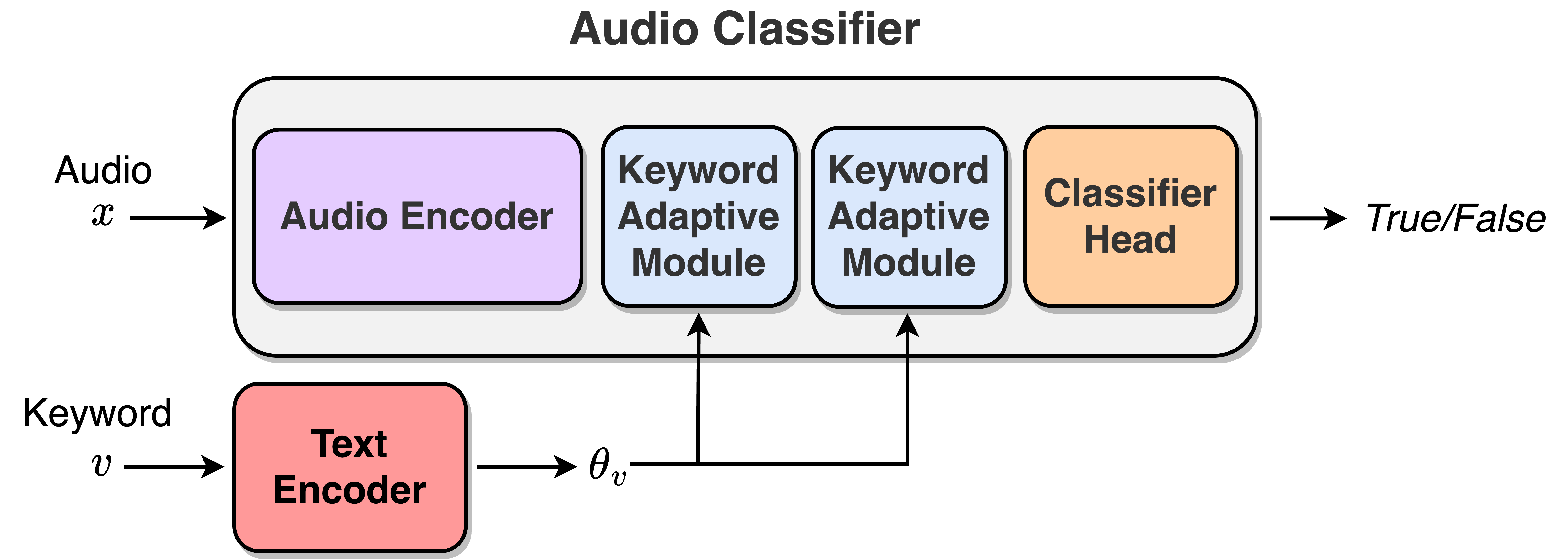
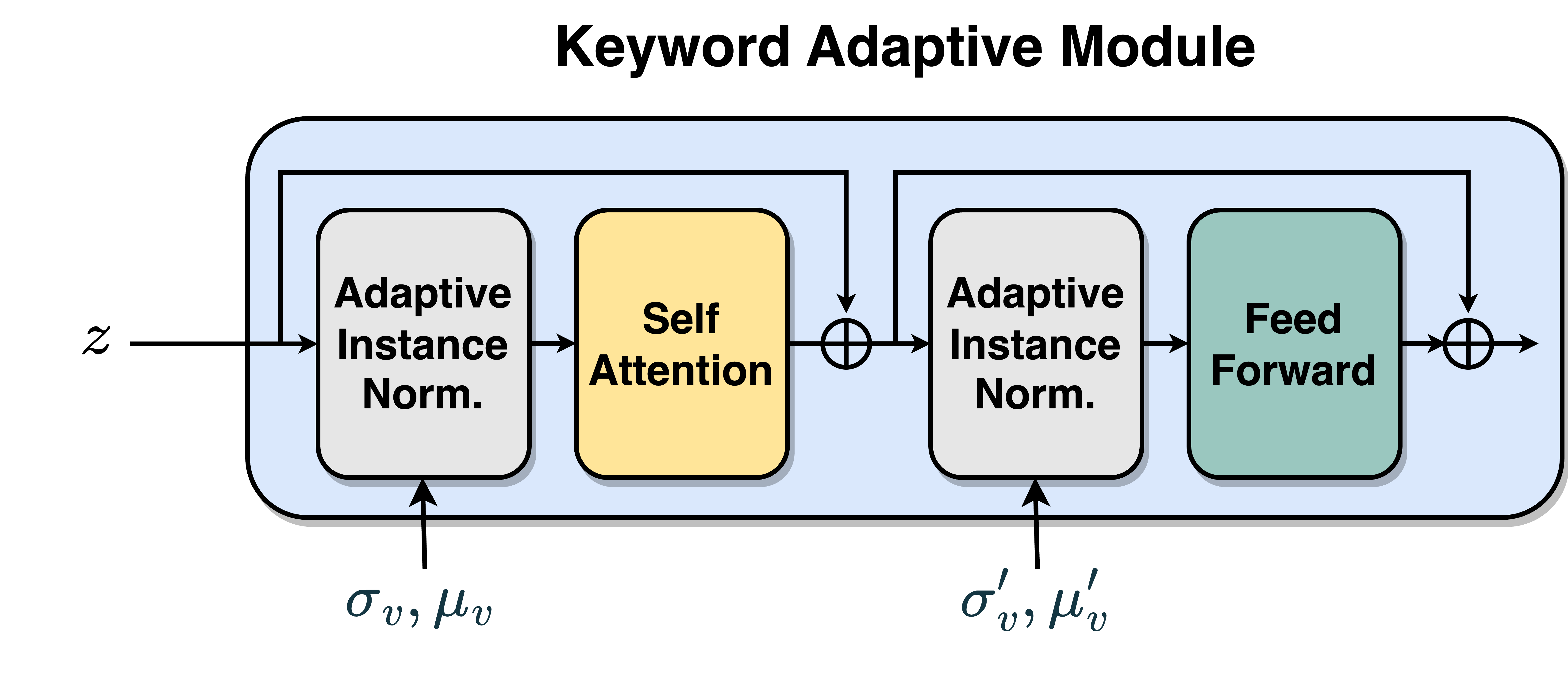
To address these issues, we take a different path to the open-vocabulary problem and propose a novel approach for KWS, termed AdaKWS. Instead of embedding textual and auditory information into a joint latent space, we employ a character-based LSTM encoder which maps an input keyword into a set of normalization parameters. These parameters are used to process the audio signal in keyword-adaptive modules (see, Figure 1). The adaptive module is a standard transformer encoder module in which we swap the Layer Normalization layers with an Adaptive Instance Normalization (AdaIN) layers [16], where the adaptive parameters are keyword-conditioned. AdaIN layers have proven highly effective for multiple tasks and domains, including image harmonization, image-to-image translation, and style editing.

To reduce the false detection of acoustically similar keywords and effectively train our model, we introduce a new technique for mining hard negative examples. Importantly, unlike previous recent works [13, 14, 15] which train the KWS model on segmented audio samples containing the keyword alone, we train our model on entire sentences (up to 30 seconds). This eliminates the need for word-level alignment or expensive preprocessing and dramatically increases the amount of available training data.

To summarize, we make the following contributions: (1) Propose a novel KWS approach, named AdaKWS, based on adaptive instance normalization layers, (2) Introduce a new technique for mining hard negative keyword examples, (3) Demonstrate the benefits and effectiveness of our approach using a diverse set of multilingual benchmarks, and generalization to unseen languages.

2 Keyword-spotting using Adaptive Instance normalization

The AdaKWS model is constructed of two main building blocks. A text encoder, and an audio classifier. The audio classifier is in turn construct of two main modules, an audio encoder, and a keyword-adaptive module (see Figure 1).

We first focus on the audio classifier, $f$. As the audio encoder, we use a pre-trained Whisper transformer encoder [17]. In our experiments, we keep the audio encoder frozen. The audio is first processed using the audio encoder, and the resulting audio representation is then passed to two sequential keyword-adaptive modules. Each module is a standard transformer encoder block in which we swap the Layer Normalization layers with Adaptive Instance Normalization layers (AdaIN). An AdaIn is a normalization layer of the form,

$$\text{AdaIN}(z,v)=\sigma_{v}\left(\frac{z-\mu_{z}}{\sigma_{z}}\right)+\mu_{v}.$$ (1)

In our case, $z$ is the audio representation and $v$ is the target keyword. Finally, the keyword-conditioned audio representation is max-pooled and fed into a linear classifier. To map the target keyword to the corresponding normalization parameters, we employ a lightweight text encoder, $h$. The text encoder is a 4-layers character-based LSTM with a $256$ hidden dimension.

More formally, let $\phi$ denote the parameters of the text encoder $h$, and let $\theta$ denote the collection of parameters in $f$ which are shared among keywords (i.e., all parameters that are not in the AdaIN layers). To detect a keyword $v$ in an auditory utterance $x$, we first process $v$ using $h$ to obtain the keyword conditioned normalization parameters $h(v;\phi)=\theta_{v}$. Here, $\theta_{v}$ denote collection of all normalization parameters $\mu(v),\sigma(v)$ from Eq. 1 Then, we determine the existence of $v$ in $x$ according to $f(x;\theta,\theta_{v}):=P(v|x)$.

Note that under the above setup, the trainable parameters are $\phi,\theta$. The text encoder parameters can be updated according to the chain rule,

$$\nabla_{\phi}\mathcal{L}(x,v)=(\nabla_{\phi}\theta_{v})^{T}\nabla_{\theta_{v}}\mathcal{L}(x,v)$$ (2)

where $\mathcal{L}$ denotes the classification loss (i.e., cross-entropy) for $(x,v)$. We summarize our training procedure in Alg. 1.

Our method, AdaKWS, provides a natural way for sharing information across keywords, through the shared parameters $(\phi,\theta)$, while maintaining the flexibility of generating diverse keyword-specific classifiers.

Algorithm 1 AdaKWS

input: $\alpha$ — Text encoder learning rate, $\eta$ — classifier learning rate, $\theta$ — Audio classifier parameters, $\phi$ — Text encoder parameters

for $r=1,...,n$ do

    sample a batch of pos/neg examples $\{(x_{i},v_{i})\}_{i=1}^{B}.$

    compute $\theta_{v_{i}}=h(v_{i};\phi)$

    $\theta=\theta-\eta\frac{1}{B}\sum_{i}\nabla_{\theta}\mathcal{L}(x_{i},v_{i})$

    $\phi=\phi-\alpha\frac{1}{B}\sum_{i}(\nabla_{\phi}\theta_{v_{i}})^{T}\nabla_{\theta_{v_{i}}}\mathcal{L}(x_{i},v_{i})$

return: $\phi,\theta$

Table 1: VoxPopuli: F1 results for the VoxPopuli test dataset.

	CS	DE	EN	ES	ET	FI	FR	HR	HU	IT	LT	NL	PL	RO	SK	SL	Overall	# Params
Whisper-Tiny	$48.5$	$77.0$	$83.4$	$85.6$	$39.5$	$58.4$	$78.3$	$48.6$	$47.0$	$72.2$	$38.4$	$67.8$	$74.7$	$52.0$	$43.8$	$46.0$	$69.3$	$39$M
Whisper-Small	$77.9$	$89.3$	$84.1$	$86.3$	$55.2$	$81.5$	$90.5$	$72.5$	$72.5$	$85.4$	$62.5$	$85.8$	$89.7$	$77.3$	$68.8$	$64.3$	$83.3$	$244$M
Whisper-Large-V2	$91.0$	$93.2$	$80.5$	$87.8$	$78.5$	$89.1$	$93.2$	$67.9$	$87.4$	$87.7$	$76.1$	$\mathbf{92.6}$	$93.8$	$87.7$	$84.0$	$80.0$	$88.4$	$1550$M
AdaKWS-Tiny	$91.8$	$94.4$	$95.5$	$95.1$	$86.2$	$92.1$	$94.9$	$89.3$	$90.6$	$90.8$	$\mathbf{85.6}$	$91.1$	$93.0$	$91.9$	$91.7$	$85.6$	$92.8$	$15$M
AdaKWS-Base	$92.3$	$95.2$	$95.9$	$95.1$	$85.2$	$92.2$	$\mathbf{96.3}$	$90.4$	$91.3$	$92.0$	$82.1$	$91.5$	$94.3$	$92.9$	$93.9$	$88.5$	$93.7$	$31$M
AdaKWS-Small	$\mathbf{94.4}$	$\mathbf{95.7}$	$\mathbf{96.3}$	$\mathbf{95.6}$	$\mathbf{91.1}$	$\mathbf{94.8}$	$95.9$	$\mathbf{93.0}$	$\mathbf{92.7}$	$\mathbf{92.8}$	$78.5$	$92.2$	$\mathbf{95.5}$	$\mathbf{94.8}$	$\mathbf{94.5}$	$\mathbf{89.9}$	$\mathbf{94.6}$	$109$M

3 Negative Sampling

In this section, we present our negative sampling approach which we employ for creating a diverse set of hard negative examples per batch.

Let $\{(x_{i},\mathbf{v}_{i})\}$ for $i=1,...,N$ denotes the training data. Here $x$ denotes the speech utterance and $\mathbf{v}=(v_{1},...,v_{M})$ denotes the corresponding transcripts, with $v_{i}\in\mathcal{V}$ for all $i$. Here $\mathcal{V}$ denotes a set of training keywords. During training, given an example $(x,\mathbf{v})$, we sample a random positive keyword $v^{+}\in\mathbf{v}$ to form a positive training example $(x,v^{+})$. In order to generate a negative training example, we consider several alternatives.
Random negative. Here we simply sample a random keyword from $v^{-}\in\mathcal{V}\setminus\mathbf{v}$. We empirically found that this simple approach is not sufficient for training a KWS model that can accurately separate acoustic similar words. Intuitively, the random sampled keywords are acoustically far from the keywords in $\mathbf{v}$.

To address this issue, we introduce several approaches for constructing hard negative examples.
Character substitution. Here, we alter a positive keyword $v^{+}$, by substituting one or more of its characters. The new character can be chosen randomly, or according to an a priori mapping of acoustically similar characters (“s”$\to$“z”,“p”$\to$“b”, etc.).
Keyword concatenation. Here we form a negative keyword by concatenating a random keyword $v\in\mathcal{V}\setminus\mathbf{v}$ to a positive keyword $v^{+}$, i.e., $v^{-}=v\circ v^{+}$ or $v^{-}=v^{+}\circ v$, where $\circ$ denotes the concatenation operator.
Nearest keyword (NK). To obtain negative keyword $v^{-}$ that are acoustically similar to a reference keyword $v^{+}$, we sample $v^{-}$ according to the text embedding representation $e(v)$. Specifically, we use the last hidden layer of $h$ to form the embedding representation. To ensure efficiency, we sample negative examples within each training batch, by querying for the keyword with the smallest cosine distance, i.e., $v^{-}=\arg\min_{v\in\mathcal{V}_{\mathcal{B}}\setminus v^{+}}d(e(v^{+}),e(v))$, where $\mathcal{V}_{\mathcal{B}}$ denotes the keywords in batch $\mathcal{B}$.

Fig. 2: Model predictions. We illustrate the predicted probability of a queried keyword (y-axis) across different time windows. Note that higher probability scores are aligned with the temporal occurrence of the word within the utterance (x-axis).

Table 2: LibriPhrase: AUC and EER results for LibriPhrase hard (LH) and easy (LE) test splits.

	AUC (%) $\uparrow$		EER (%) $\downarrow$
	LH	LE	LH	LE
Triplet [12]	$54.88$	$63.53$	$44.36$	$32.75$
Attention [11]	$62.65$	$78.74$	$41.95$	$28.74$
DONUT [10]	$54.88$	$63.53$	$44.36$	$32.75$
CMCD [13]	$73.58$	$96.70$	$32.90$	$8.42$
EMKWS [14]	$84.21$	$97.83$	$23.36$	$7.36$
CED [15]	$92.70$	$\mathbf{99.84}$	$14.40$	$1.70$
AdaKWS-Tiny	$93.75$	$99.80$	$13.47$	$1.61$
AdaKWS-Base	$94.39$	$99.81$	$12.60$	$1.37$
AdaKWS-Small	$\mathbf{95.09}$	$99.82$	$\mathbf{11.48}$	$\mathbf{1.21}$

4 Experiments

Table 3: Multilingual-LibriSpeech: Zero-shot F1 results for the Multilingual-LibriSpeech test dataset.

	DE	EN	ES	FR	IT	NL	PL	Overall	# Params	Inference Time (MS) $\downarrow$
Whisper-Tiny	$77.6$	$85.8$	$83.6$	$73.4$	$72.4$	$69.2$	$76.0$	$77.9$	$39$M	$260$
Whisper-Small	$90.8$	$91.3$	$92.9$	$88.2$	$85.8$	$86.1$	$91.5$	$89.6$	$244$M	$621$
Whisper-Large-V2	$\mathbf{95.0}$	$\mathbf{93.8}$	$\mathbf{95.1}$	$93.8$	$91.7$	$\mathbf{92.3}$	$\mathbf{95.2}$	$\mathbf{93.9}$	$1550$M	$1836$
AdaKWS-Tiny	$92.6$	$91.4$	$92.1$	$91.9$	$92.3$	$87.9$	$92.6$	$91.3$	$15$M	$6$
AdaKWS-Base	$93.8$	$92.6$	$92.2$	$92.8$	$92.7$	$90.0$	$92.8$	$92.4$	$31$M	$7$
AdaKWS-Small	$94.6$	$\mathbf{93.8}$	$94.4$	$\mathbf{94.1}$	$\mathbf{94.2}$	$91.8$	$94.4$	$93.8$	$109$M	$11$

In this section, we compare AdaKWS with various KWS approaches on different learning setups and datasets. The experiments show the superiority of AdaKWS over previous KWS methods.
Datasets. We use several datasets. VoxPopuli [18]: A large-scale multilingual speech corpus collected from the European parliament, with $\sim 1800$ hours of transcribed utterances from $16$ languages. LibriPhrase [13]: A recent benchmark for KWS based on the LibriSpeech [19] dataset. It consists of two splits, LibriPhrase Hard (LH) and LibriPhrase Easy (LE). Furthermore, we evaluate our model using two additional datasets, Multilingual LibriSpeech and Fluers [20]. To construct our evaluation set, we first randomly sample positive keywords. Then, we sample random, concat, and swap negatives as described in Section 3, with equal probability. This results in a diverse and challenging open-vocabulary KWS benchmark.
Experimental setup. The AdaKWS models are trained using the VoxPopuli dataset for $25$ epochs with batch-size $144$ and $1e-4$ learning rate. We train three variants with varying audio encoder sizes, Tiny, Base, and Small, corresponding to the frozen Whisper encoder (audio encoder, Figure 1). We report common metrics in the KWS field, namely F1 score, Area Under the Curve (AUC), and Equal Error Rate (ERR).
Data preprocessing. We follow the data processing procedure from [17]. Each audio instance is resampled to a frequency of 16KHz, then an 80-channel log-magnitude Mel spectrogram representation is generated using 25-millisecond windows and 10-millisecond strides.
Baselines. We compare AdaKWS with recent keyword spotting and ASR works. The compared methods include: (1) Whisper [17] - We transcribe the input audio into text and subsequently conduct a search to ascertain the presence of the desired keyword within the output text. (2) CED [15] - flexible KWS method using audio-compliant text encoder. (3) EMKWS [14] - contrastive learning approach using text-audio embedding matching. (4) CMCD [13] - fusing the text and audio representation to shared latent space using cross-modal attention. Additional query by example methods (5) DONUT [10], (6) Attention [11], and (7) Triplet [12].

Table 4: Zero-shot performance for low resource, novel languages: F1 results for four novel and low resources languages from the Fleurs test dataset.

	Icelandic	Maltese	Swahili	Uzbek	Overall
Whisper-Tiny	$42.3$	$37.6$	$43.9$	$34.2$	$37.8$
Whisper-Small	$52.0$	$34.9$	$55.6$	$35.4$	$40.4$
Whisper-Large-V2	$69.2$	$38.6$	$\mathbf{74.9}$	$36.6$	$48.1$
AdaKWS-Tiny	$69.2$	$\mathbf{76.7}$	$70.1$	$\mathbf{67.5}$	$\mathbf{71.9}$
AdaKWS-Base	$\mathbf{71.5}$	$\mathbf{76.7}$	$71.6$	$65.7$	$71.6$
AdaKWS-Small	$70.6$	$76.0$	$69.4$	$66.1$	$70.9$

4.1 Main Results

We start with evaluating AdaKWS on the VoxPopuli dataset. The results are presented in Table 1. AdaKWS outperforms the Whisper baselines by a notable margin, over $6\%$ w.r.t the best performing baseline. Moreover, AdaKWS outperforms the baselines in $15$ of $16$ languages with $\sim 10\times$ fewer parameters. We follow the protocol from [13, 15, 14] and evaluate AdaKWS on the LibriPhrase dataset. We use AdaKWS pre-trained on VoxPopuli and fine-tune it using $30K$ samples from the LibriPhrase training set for an additional $10$ epochs. The results are presented in Table  2. AdaKWS significantly outperforms the current SOTA method on the challenging LibriPhrase Hard benchmark.

4.2 Generalization to Novel Languages and Datasets

We further investigate the generalization ability of AdaKWS in two ways: Adapting to novel, low-resource languages, and generalizing to datasets that are not utilized during training. For both experiments, we use AdaKWS trained on the VoxPopuli dataset from Section 4.1 without fine-tuning. First, we evaluate the pre-trained AdaKWS on a subset of $4$ languages randomly drawn from Fleurs [20], which share the same character set observed during training. Second, we evaluate how well AdaKWS generalizes to unseen utterances from the multilingual LibriSpeech (MLS) [19] dataset. We also report the inference time for each model estimated using a single V$100$ Nvidia GPU, averaged using $1000$ random samples. The results are presented in Tables 4 and 3. For MLS, our AdaKWS-Small model achieves on-par performance with $\sim 160$x faster inference time, w.r.t the Whisper large-v2 baseline.

4.3 Ablation Study

We empirically investigate the effects of distinct negative sampling methods on the performance of our model on the Voxpopuli dataset. The results presented in Table 5 showcase the importance of the proposed negative sampling approach for AdaKWS performance.

Table 5: Negative sampling: Results for the AdaKWS-tiny model, trained using different negative sampling approaches, on the VoxPopuli test dataset.

	F1 $\uparrow$	AUC $\uparrow$	EER $\downarrow$
Random	$79.37$	$88.09$	$19.37$
Random + NK	$81.24$	$88.79$	$18.80$
Random + NK + Cat.	$84.99$	$91.20$	$15.91$
Random + NK + Cat. + Swap	$\mathbf{92.87}$	$\mathbf{97.78}$	$\mathbf{7.16}$

5 Conclusion

In this paper, we present AdaKWS, a novel approach for keyword spotting. Our model employs a keyword adaptive instance normalization layer which allows the model to adapt to novel keywords during inference. Along with the introduced negative keyword mining approach, AdaKWS achieves state-of-the-art results in challenging open-vocabulary multilingual setups. Furthermore, we demonstrate the generalization abilities of AdaKWS to adapt to unseen languages and datasets. The impressive achievements of AdaKWS not only advance the current state-of-the-art but also pave the way for future research in this domain.

References

- [1] Iván López-Espejo, Zheng-Hua Tan, John HL Hansen, and Jesper Jensen, “Deep spoken keyword spotting: An overview,” IEEE Access, vol. 10, pp. 4169–4199, 2021.
- [2] Tzeviya Sylvia Fuchs, Yael Segal, and Joseph Keshet, “Cnn-based spoken term detection and localization without dynamic programming,” in ICASSP 2021-2021 IEEE International Conference on Acoustics, Speech and Signal Processing (ICASSP). IEEE, 2021, pp. 6853–6857.
- [3] Axel Berg, Mark O’Connor, and Miguel Tairum Cruz, “Keyword transformer: A self-attention model for keyword spotting,” arXiv preprint arXiv:2104.00769, 2021.
- [4] Somshubra Majumdar and Boris Ginsburg, “Matchboxnet: 1d time-channel separable convolutional neural network architecture for speech commands recognition,” arXiv preprint arXiv:2004.08531, 2020.
- [5] Kevin Ding, Martin Zong, Jiakui Li, and Baoxiang Li, “Letr: A lightweight and efficient transformer for keyword spotting,” in ICASSP 2022-2022 IEEE International Conference on Acoustics, Speech and Signal Processing (ICASSP). IEEE, 2022, pp. 7987–7991.
- [6] Paul M Reuter, Christian Rollwage, and Bernd T Meyer, “Multilingual query-by-example keyword spotting with metric learning and phoneme-to-embedding mapping,” in ICASSP 2023-2023 IEEE International Conference on Acoustics, Speech and Signal Processing (ICASSP). IEEE, 2023, pp. 1–5.
- [7] Dongjune Lee, Minchan Kim, Sung Hwan Mun, Min Hyun Han, and Nam Soo Kim, “Fully unsupervised training of few-shot keyword spotting,” in 2022 IEEE Spoken Language Technology Workshop (SLT). IEEE, 2023, pp. 266–272.
- [8] R Kirandevraj, Vinod K Kurmi, Vinay P Namboodiri, and CV Jawahar, “Generalized keyword spotting using asr embeddings,” in 23rd Annual Conference of the International Speech Communication Association, INTERSPEECH 2022. ISCA, 2022, pp. 126–130.
- [9] Jaemin Jung, Youkyum Kim, Jihwan Park, Youshin Lim, Byeong-Yeol Kim, Youngjoon Jang, and Joon Son Chung, “Metric learning for user-defined keyword spotting,” in ICASSP 2023-2023 IEEE International Conference on Acoustics, Speech and Signal Processing (ICASSP). IEEE, 2023, pp. 1–5.
- [10] Loren Lugosch, Samuel Myer, and Vikrant Singh Tomar, “Donut: Ctc-based query-by-example keyword spotting,” ArXiv, vol. abs/1811.10736, 2018.
- [11] Jinmiao Huang, Waseem Gharbieh, Han Suk Shim, and Eugene Kim, “Query-by-example keyword spotting system using multi-head attention and soft-triple loss,” ICASSP 2021 - 2021 IEEE International Conference on Acoustics, Speech and Signal Processing (ICASSP), pp. 6858–6862, 2021.
- [12] Niccolo Sacchi, Alexandre Nanchen, Martin Jaggi, and Milos Cernak, “Open-vocabulary keyword spotting with audio and text embeddings,” in INTERSPEECH 2019-IEEE International Conference on Acoustics, Speech, and Signal Processing, 2019, number CONF.
- [13] Hyeon-Kyeong Shin, Hyewon Han, Doyeon Kim, Soo-Whan Chung, and Hong-Goo Kang, “Learning audio-text agreement for open-vocabulary keyword spotting,” arXiv preprint arXiv:2206.15400, 2022.
- [14] Kumari Nishu, Minsik Cho, and Devang Naik, “Matching latent encoding for audio-text based keyword spotting,” arXiv preprint arXiv:2306.05245, 2023.
- [15] Kumari Nishu, Minsik Cho, Paul Dixon, and Devang Naik, “Flexible keyword spotting based on homogeneous audio-text embedding,” arXiv preprint arXiv:2308.06472, 2023.
- [16] Xun Huang and Serge J. Belongie, “Arbitrary style transfer in real-time with adaptive instance normalization,” 2017 IEEE International Conference on Computer Vision (ICCV), pp. 1510–1519, 2017.
- [17] Alec Radford, Jong Wook Kim, Tao Xu, Greg Brockman, Christine McLeavey, and Ilya Sutskever, “Robust speech recognition via large-scale weak supervision,” ArXiv, vol. abs/2212.04356, 2022.
- [18] Changhan Wang, Morgane Rivière, Ann Lee, Anne Wu, Chaitanya Talnikar, Daniel Haziza, Mary Williamson, Juan Miguel Pino, and Emmanuel Dupoux, “Voxpopuli: A large-scale multilingual speech corpus for representation learning, semi-supervised learning and interpretation,” in Annual Meeting of the Association for Computational Linguistics, 2021.
- [19] Vassil Panayotov, Guoguo Chen, Daniel Povey, and Sanjeev Khudanpur, “Librispeech: An asr corpus based on public domain audio books,” 2015 IEEE International Conference on Acoustics, Speech and Signal Processing (ICASSP), pp. 5206–5210, 2015.
- [20] Alexis Conneau, Min Ma, Simran Khanuja, Yu Zhang, Vera Axelrod, Siddharth Dalmia, Jason Riesa, Clara Rivera, and Ankur Bapna, “Fleurs: Few-shot learning evaluation of universal representations of speech,” 2022 IEEE Spoken Language Technology Workshop (SLT), pp. 798–805, 2022.